Cooperative Environmental Monitoring
for PTZ Visual Sensor Networks:
A Payoff-based Learning Approach

Abstract

This paper investigates cooperative environmental monitoring for Pan-Tilt-Zoom (PTZ) visual sensor networks. We first present a novel formulation of the optimal environmental monitoring problem, whose objective function is intertwined with the uncertain state of the environment. In addition, due to the large volume of vision data, it is desired for each sensor to execute processing through local computation and communication. To address the issues, we present a distributed solution to the problem based on game theoretic cooperative control and payoff-based learning. At the first stage, a utility function is designed so that the resulting game constitutes a potential game with potential function equal to the group objective function, where the designed utility is shown to be computable through local image processing and communication. Then, we present a payoff-based learning algorithm so that the sensors are led to the global objective function maximizers without using any prior information on the environmental state. Finally, we run experiments to demonstrate the effectiveness of the present approach.

I Introduction

Large-scale environmental monitoring to reveal environmental states has become crucial due to recent serious natural disasters including earthquakes, tsunamis, nuclear meltdowns, landslides, typhoons/hurricanes and so on. In the task, it is in general required to collect dense data in real time over widespread environment. As a solution to the issue, sensor networks have emerged over the past few decades and been extensively studied. Moreover, mobile/robotic sensor networks have also been deeply investigated as a key technology to enhance data collection efficiency [1].

Among a variety of sensors available for the monitoring task [1], this paper focuses on vision sensors. In particular, we consider a sensor network consisting of spatially distributed cameras, which is called camera/visual sensor network [2]. Then, we need to take account of the following nature of vision sensors: (i) volume of data tends to be larger than the other sensors, (ii) vision sensors do not provide explicit physical data, and (iii) vision sensors are inherently heterogeneous, which means that, even if quality of two sensors are the same, quality of their measurements on a common point can differ in the location of the point relative to the camera frames.

In this paper, we investigate a distributed/cooperative optimal monitoring strategy for a network of Pan-Tilt-Zoom (PTZ) cameras by controlling the camera parameters, which are called actions in this paper. Note that what is the optimal action in the problem is affected by the unknown environmental state. Accordingly, we have to solve the optimization problem under the restriction: (iv) each vision sensor has no access to the reward brought about by an action before the action is actually executed. Optimization under (iv) has been deeply studied in the field of reinforcement learning and simulated annealing. However, these algorithms are centralized and might not be available due to the nature (i).

This paper first formulates a novel optimal environmental monitoring problem for PTZ visual sensor networks reflecting the nature (ii) and (iii), where we let the objective function rely on the amount of information contained in the sensed data and the quality of the measurement. Then, we next present a distributed solution to the problem leading the sensors to the globally optimal actions under the restriction of (iv). To meet the requirements, this paper employs techniques in game theoretic cooperative control originally presented in [3] since it provides a systematic design procedure of cooperative control for heterogeneous networks as stated in (iii). Following the procedure of [3], we first constitute a potential game [3] with the potential function equal to the global objective function through an appropriate utility design technique [4]. Then, as a technical tool to address (iv), we employ an action selection rule called payoff-based learning [5]–[8], where each player chooses his action based only on the past experienced payoffs. In particular, we present a novel payoff-based learning algorithm which guarantees convergence in probability to the potential function maximizers, which are equal to the global objective function maximizers. Finally, we run experiments on a visual sensor network testbed to demonstrate the effectiveness of the present approach.

Related Works and Contributions

Due to the nature of vision sensors (i), distributed processing over visual sensor networks has been actively studied in some recent papers. Cooperative estimation over visual sensor networks is studied in [9], [10], [11], distributed localization/calibration is investigated in [11], [12], and distributed sensing strategies are presented in [13], [14], [15]. In particular, the scenarios and approaches in [13], [14] are closely related to this paper and hence they will be mentioned later.

The objective of this paper is related to coverage control [16]–[21] whose objective is to deploy mobile sensors efficiently via distributed decision-making. A gradient decent approach widely used in the literature [16, 17] is implementable even under the restriction (iv). However, the approach is not always directly applicable to the problem of this paper due to the nature of vision sensors (ii) and (iii). More importantly, the gradient decent approach leads sensors to a configuration achieving local maxima of some group objective function, but such a configuration does not always globally maximize the objective function.

Persistent monitoring is also recently studied e.g. in [22]–[25], which differs from coverage in the perpetual need to cover a changing environment [24, 25]. However, to the best of our knowledge, there are few works fully taking account of the nature of vision sensors. In addition, while most of the works [23]–[25] assume information accumulation/decay models and availability of the model, this paper does not presume such models.

The papers [3, 13, 14, 21] are most directly related to this paper, where the authors investigate potential game theoretic approaches to coverage control or collaborative sensing. The algorithm presented in [3] guarantees that players eventually take the globally optimal action with high probability. However, it presumes availability of future payoffs prior to action executions and hence cannot be implemented under (iv). [14] presents a payoff-based learning algorithm and applied it to coverage for visual (mobile) sensor networks. However, the algorithm does not always lead sensors to the globally optimal actions and the nature (ii) and (iii) are not fully addressed. Similar statements are also true for [21]. Meanwhile, [13] mentions how to use the visual measurement in the process explicitly. Though the authors utilize a learning algorithm assuming a future payoff, they successfully avoid the issue (iv) by constructing the future virtual utility from the estimate of the target states produced by a distributed filter. However, the approach may limit applications since there might be no explicit target in some scenarios.

We finally mention the contribution of the present learning algorithm. The algorithm is regarded as a variation of [5] and [14]. [5] guarantees that potential function maximizers are eventually selected with high probability. Meanwhile, [14] has advantages over [5] that the action selection rule is simpler and convergence in probability is rigorously guaranteed, but it does not always lead sensors to potential function maximizers. The contribution of the present algorithm is to embody advantages of these two algorithms, i.e. guarantees convergence in probability to potential function maximizers while maintaining the simple structure of [14].

The contributions of this paper are summarized as follows:

• a novel problem formulation of environmental monitoring for PTZ visual sensor networks taking account of the nature of vision sensors (ii) and (iii) is presented,

• a novel simple payoff-based learning algorithm for potential games guaranteeing convergence in probability to the potential function maximizers is proposed, and

• the approach is demonstrated through experiments, while such efforts are not always fully made in the existing works on game theoretic cooperative control.

II Visual Sensor Networks and Environment

II-A Visual Sensor Networks and Environment

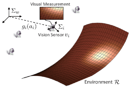
Figure 1: Targeted scenario

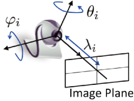
Figure 2: Actions of vision sensor $v_{i}$

In this paper, we consider the situation illustrated in Fig. 2, where $n$ Pan-Tilt-Zoom (PTZ) vision sensors ${\mathcal{V}}=\{v_{1},\cdots,v_{n}\}$ monitor environment modeled by a collection of $m$ polygons ${\mathcal{R}}=\{r_{1},\cdots,r_{m}\}$. Let the set of position vectors of all points in $r_{j}\in{\mathcal{R}}$ relative to a world frame $\Sigma_{w}$ be denoted by ${\mathcal{Q}}_{j}$. In the following, we also use the notation ${\mathcal{Q}}=\cup_{r_{j}\in{\mathcal{R}}}{\mathcal{Q}}_{j}$.

Suppose that each PTZ vision sensor $v_{i}\in{\mathcal{V}}$ can adjust its horizontal (pan) angle $\theta_{i}\in\varTheta_{i}\subseteq[-\pi,\pi]$, vertical (tilt) angle $\varphi_{i}\in\varPhi_{i}\subseteq[0,\pi]$ and focal length $\lambda_{i}\in\varLambda_{i}$ (Fig. 2), where $\varTheta_{i},\varPhi_{i}$ and $\varLambda_{i}$ are assumed to be finite sets. Throughout this paper, the notation

$$a_{i}=(\theta_{i},\varphi_{i},\lambda_{i})\in{\mathcal{A}}_{i}:=\varTheta_{i}\times\varPhi_{i}\times\varLambda_{i}$$

is called an action of sensor $v_{i}\in{\mathcal{V}}$, and $a=(a_{i})_{v_{i}\in{\mathcal{V}}}\in{\mathcal{A}}:={\mathcal{A}}_{1}\times\cdots\times{\mathcal{A}}_{n}$ is called a joint action. A collection of actions other than $v_{i}$ is denoted as $a_{-i}:=(a_{1},\cdots,a_{i-1},a_{i+1},\cdots,a_{n})$.

Once an action $a_{i}$ is fixed, the orientation of sensor $v_{i}$’s frame $\Sigma_{i}$ relative to $\Sigma_{w}$ and its maximal view angle are uniquely determined, which are respectively denoted by $R_{i}(a_{i})\in SO(3):=\{R\in{\mathbb{R}}^{3\times 3}|\ R^{T}R=I_{3},\ \det(R)=+1\}$ and $\bar{\beta}_{i}(a_{i})$. The position of the origin of $\Sigma_{i}$ relative to $\Sigma_{w}$ is also denoted by $p_{i}\in{\mathbb{R}}^{3}$. Then, the pose of sensor $v_{i}$ is represented as $g_{i}(a_{i})=(p_{i},R_{i}(a_{i}))\in SE(3):={\mathbb{R}}^{3}\times SO(3)$. In this paper, we assume that each $v_{i}\in{\mathcal{V}}$ is already calibrated and has knowledge on the pose $g_{i}(a_{i})$ for all $a_{i}\in{\mathcal{A}}$, and ${\mathcal{Q}}_{j}=\{q\in{\mathbb{R}}^{3}|\ A_{{\rm eq},j}q=1,\ A_{{\rm ieq},j}q\leq{\bf 1}\}$ for all $r_{j}\in{\mathcal{R}}$, where ${\bf 1}$ is a vector whose elements are all equal to $1$.

We also assume that, when each sensor $v_{i}\in{\mathcal{V}}$ takes action $a_{i}\in{\mathcal{A}}_{i}$, the actions selectable at the next round are constrained by a subset ${\mathcal{C}}_{i}(a_{i})\subseteq{\mathcal{A}}_{i}$ satisfying the following assumptions which are in general satisfied in the scenario of this paper.

Assumption 1

The function ${\mathcal{C}}_{i}:{\mathcal{A}}_{i}\rightarrow 2^{{\mathcal{A}}_{i}}$ satisfies:

• For any $v_{i}\in{\mathcal{V}}$, $a_{i}\in{\mathcal{A}}_{i}$ and $a^{\prime}_{i}\in{\mathcal{A}}_{i}$, the inclusion $a^{\prime}_{i}\in{\mathcal{C}}_{i}(a_{i})$ holds iff $a_{i}\in{\mathcal{C}}_{i}(a^{\prime}_{i})$.

• For any $v_{i}\in{\mathcal{V}}$ and any actions $a_{i},a^{\prime}_{i}\in{\mathcal{A}}_{i}$, there exists a sequence of actions $a_{i}=a_{i}^{1},a_{i}^{2},\cdots,a^{n_{f}}_{i}=a_{i}^{\prime}$ satisfying $a_{i}^{\iota}\in{\mathcal{C}}_{i}(a_{i}^{\iota-1})$ for all $\iota\in\{2,\cdots,n_{f}\}$.

• For any $v_{i}\in{\mathcal{V}}$ and $a_{i}\in{\mathcal{A}}_{i}$, the number of elements in ${\mathcal{C}}_{i}(a_{i})$ is greater than or equal to $3$.

II-B Visual Measurements and Communication Structure

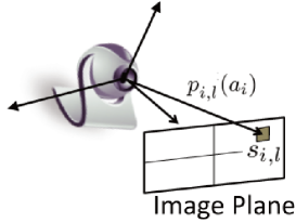
Figure 3: Position vector $p_{i,l}(a_{i})$ of pixel $s_{i,l}$

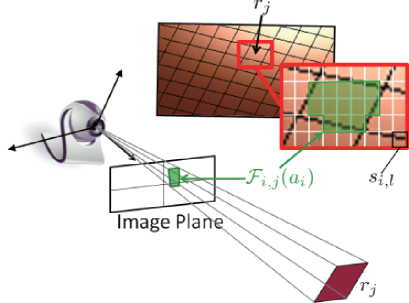
Figure 4: Image of set ${\mathcal{F}}_{i,j}(a_{i})$

This subsection defines visual measurements of each vision sensor $v_{i}\in{\mathcal{V}}$ and communication structures among sensors in ${\mathcal{V}}$.

Let us first denote the pixels of vision sensor $v_{i}\in{\mathcal{V}}$ by ${\mathcal{S}}_{i}:=\{s_{i,l}|\ l\in\{1,\cdots,S_{i}\}\}$, and the position vector of the center of $s_{i,l}\in{\mathcal{S}}_{i}$ relative to $\Sigma_{i}$ by $p_{i,l}(a_{i})$ (Fig. 4). Then, once an action $a_{i}$ is fixed, $v_{i}$ obtains visual measurements (raw data) $y_{i,l}$ for each $s_{i,l}\in{\mathcal{S}}_{i}$. Here, $y_{i,l}$ is a 3D vector for an RGB color image whose elements take integers in $\{0,\cdots,255\}$, and $y_{i,l}\in\{0,\cdots,255\}$ for a grey-scale image. Note that each $y_{i,l}$ is provided by either of polygons $r_{j}\in{\mathcal{R}}$.

In this paper, a point $q\in{\mathcal{Q}}$ is said to be visible from sensor $v_{i}\in{\mathcal{V}}$ with action $a_{i}\in{\mathcal{A}}$ if

$${\rm atan}(\|[b_{x}\ b_{y}]\|/b_{z})\leq\bar{\beta}_{i}(a_{i}),\ [b_{x}\ b_{y}\ b_{z}]^{T}:=R_{i}^{T}(a_{i})(q-p_{i})$$

and there exists no pair of $q^{\prime}\in{\mathcal{Q}}$ and $\alpha\in[0,1)$ such that $\alpha(q-p_{i})=q^{\prime}-p_{i}$. By using the notion, we also define the set of pixels of $v_{i}\in{\mathcal{V}}$ with $a_{i}\in{\mathcal{A}}_{i}$ capturing $r_{j}\in{\mathcal{R}}$, which is denoted by ${\mathcal{F}}_{i,j}(a_{i})$ (Fig. 4). Here, a pixel $s_{i,l}\in{\mathcal{S}}_{i}$ is a member of ${\mathcal{F}}_{i,j}(a_{i})$ if and only if there exists a visible point $q\in{\mathcal{Q}}_{j}$ such that the point $q$ projected onto the image plane is equal to the center of the pixel $s_{i,l}$. Due to the knowledge of $g_{i}(a_{i})$ and ${\mathcal{Q}}_{j}$, each $v_{i}\in{\mathcal{V}}$ can obtain ${\mathcal{F}}_{i,j}(a_{i})$ for every $a_{i}\in{\mathcal{A}}_{i}$. To be precise, a pixel $s_{i,l}$ is included in ${\mathcal{F}}_{i,j}(a_{i})$ if $r_{j}$ satisfies

$$\alpha_{i,j}(a_{i})=\frac{1-A_{{\rm eq},j}p_{i}}{A_{{\rm eq},j}R_{i}(a_{i})p_{i,l}(a_{i})}\in(0,\infty),\ A_{{\rm ine},j}\left(\alpha_{i,j}(a_{i})R_{i}(a_{i})p_{i,l}(a_{i})+p_{i}\right)\leq{\bf 1}$$ (1)

and the parameter $\alpha_{i,j}(a_{i})$ is minimal among all polygons satisfying (1).

In addition, a polygon $r_{j}\in{\mathcal{R}}$ is said to be a visible polygon from sensor $v_{i}\in{\mathcal{V}}$ with $a_{i}\in{\mathcal{A}}_{i}$ if $|{\mathcal{F}}_{i,j}(a_{i})|\geq 1$, where $|{\mathcal{F}}|$ specifies the number of elements of a finite set ${\mathcal{F}}$. We also denote the set of all visible polygons from $v_{i}$ with $a_{i}$ by ${\mathcal{R}}_{i}(a_{i})\subseteq{\mathcal{R}}$. In addition, when a joint action $a$ is selected, the set of sensors capturing $r_{j}$ as a visible polygon is denoted by ${\mathcal{V}}_{j}(a)\subseteq{\mathcal{V}}$.

We also model the communication structure among sensors by an undirected graph $G=({\mathcal{V}},\ {\mathcal{E}})$ with ${\mathcal{E}}\subseteq{\mathcal{V}}\times{\mathcal{V}}$. The set of all sensors whose information is available for $v_{i}\in{\mathcal{V}}$ is also denoted as ${\mathcal{N}}_{i}:=\{v_{j}\in{\mathcal{V}}|\ (v_{i},v_{j})\in{\mathcal{E}}\}$. In this paper, we use the following assumption.

Assumption 2

A pair $(v_{i},v_{i^{\prime}}),\ i\neq i^{\prime}$ satisfies $(v_{i},v_{i^{\prime}})\in{\mathcal{E}}$ if there exist $a_{i}\in{\mathcal{A}}_{i}$, $a_{i^{\prime}}\in{\mathcal{A}}_{i^{\prime}}$ and $r_{j}\in{\mathcal{R}}$ such that $r_{j}\in{\mathcal{R}}_{i}(a_{i})\cap{\mathcal{R}}_{i^{\prime}}(a_{i^{\prime}})$.

This assumption means that if any pair of two sensors can capture a common polygon then they need to communicate with each other, which is essentially similar to [9] and the only slight difference in description stems from whether multi-hop communication is taken into account.

III Global Objective and Utility Function

III-A Global Objective Function

Let us formulate the global objective function $W(a)\in[0,\infty)$ to be maximized by vision sensors ${\mathcal{V}}$. For this purpose, we first introduce a function $W_{i,j}(a_{i})\in[0,\infty)$ evaluating the value of measurements ${\mathcal{Y}}_{i,j}(a_{i})$ of sensor $v_{i}\in{\mathcal{V}}$ about polygon $r_{j}\in{\mathcal{R}}$.

Let us assume that the function $W_{i,j}(a_{i})$ relies on (a) how much information $r_{j}\in{\mathcal{R}}$ contains, and (b) quality of the image. Formally, if the quantitative values of factors (a) and (b) are denoted by $I^{\rm info}_{i,j}(a_{i})\in[0,\infty)$ and $I^{\rm qual}_{i,j}(a_{i})\in[0,\infty)$ respectively, the function $W_{i,j}(a_{i})$ is described as

$$W_{i,j}(a_{i})=\tilde{W}_{i,j}(I^{\rm info}_{i,j}(a_{i}),I_{i,j}^{\rm qual}(a_{i})).$$ (2)

In general, the function $\tilde{W}_{i,j}(\cdot,\cdot)$ is non-decreasing with respect to both $I^{\rm info}_{i,j}(a_{i})$ and $I^{\rm qual}_{i,j}(a_{i})$, and the equation $I^{\rm info}_{i,j}(a_{i})=I^{\rm qual}_{i,j}(a_{i})=0$ holds if $r_{j}$ is not visible from $v_{i}$, i.e. $r_{j}\notin{\mathcal{R}}_{i}(a_{i})$.

The functions $I^{\rm info}_{i,j}(a_{i})$ and $I^{\rm qual}_{i,j}(a_{i})\in[0,\infty)$ respectively play roles similar to the density function and the sensing performance function in coverage control [16], [17]. However, there are some differences. Since vision sensors do not provide apparent physical quantity like temperature or pressure, we need to extract the amount of information contained in the raw data ${\mathcal{Y}}_{i,j}(a_{i})$, which makes the selection of $I^{\rm info}_{i,j}(a_{i})$ non-trivial. However, fortunately, there are rich literature on information extraction from visual measurements, and we can freely choose one of them depending on the targeted scenario. Some examples will be shown in the next subsection. However, such quantities can be extracted after gaining the visual measurement and, moreover, the function $I^{\rm info}_{i,j}(a_{i})$ is dependent on the state of the highly uncertain environment regardless of its selection. Hence, we cannot assume availability of the value $I^{\rm info}_{i,j}(a_{i})$ prior to execution of $a_{i}$. Due to the problem, we will present a solution using only the past experienced values of $I^{\rm info}_{i,j}(a_{i})$ and $I^{\rm qual}_{i,j}(a_{i})$ in the subsequent sections.

For visual sensor networks, the quality $I^{\rm qual}_{i,j}(a_{i})$ is determined not only by the distance between $v_{i}$ and $r_{j}$ but also by their relative pose and the focal length $\lambda_{i}$, which makes the function complex. However, since the present solution does not require to model the function differently from coverage control [16], [17], it is sufficient to evaluate the quality after gaining the image. For example, using the fraction over the image that $r_{j}$ occupies as $I^{\rm qual}_{i,j}(a_{i})=f^{\rm qual}(|{\mathcal{F}}_{i,j}(a_{i})|/S_{i})$ with an increasing function $f^{\rm qual}$ satisfying $f^{\rm qual}(0)=0$ can be a useful option.

We next consider the reward $W_{j}(a)\in[0,\infty)$ provided from environment $r_{j}$ to not a single sensor $v_{i}$ but the visual sensor network ${\mathcal{V}}$. We assume that $W_{j}(a)$ is a function of $W_{i,j}(a_{i})$ only for vision sensors in ${\mathcal{V}}_{j}(a)$ capturing $r_{j}$ as

$$W_{j}(a)=\tilde{W}_{j}((W_{i,j}(a_{i}))_{v_{i}\in{\mathcal{V}}_{j}(a)})$$ (3)

with $W_{j}(a)=0$ if ${\mathcal{V}}_{j}(a)=\emptyset$ and that vision sensors ${\mathcal{V}}$ share the information of the function $\tilde{W}_{j}$. In the following, we show only two typical selections of such functions. The first option is

$$W_{j}(a)=\max_{v_{i}\in{\mathcal{V}}_{j}(a)}W_{i,j}(a_{i})$$ (4)

imposing no value on the information ${\mathcal{Y}}_{i,j}(a_{i})$ of sensor $v_{i}$ if other sensor has better measurements on $r_{j}$. The second option is to employ the function

$$W_{j}(a)=h\Big{(}\sum_{v_{i}\in{\mathcal{V}}_{j}(a)}W_{i,j}(a_{i})\Big{)}$$ (5)

for a monotonically increasing concave function $h$ with $h(0)=0$. This function weakly accepts the value of the measurement which is not the best among the sensors.

The goal of this paper is to present a cooperative/distributed action selection algorithm leading vision sensors ${\mathcal{V}}$ to a joint action $a$ maximizing the global objective function defined by

$$W(a)=\sum_{r_{j}\in{\mathcal{R}}}W_{j}(a)$$ (6)

under the constraint that $I^{\rm info}_{i,j}(a_{i})$ and $I^{\rm qual}_{i,j}(a_{i})$ are available only after $v_{i}$ executes an action $a_{i}$.

III-B Examples of Function $I^{\rm info}_{i,j}$

Figure 5: Initial image

Figure 6: Current image

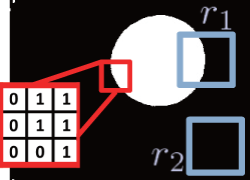
Figure 7: Outputs of function $I^{\rm ec}_{i,l}$

In this subsection, we will introduce examples of the function $I^{\rm info}_{i,j}(a_{i})$.

We first consider a normally static environment, and suppose that we are interested only in whether or not each pixel $s_{i,l}$ captures environmental changes. The requirement is reflected by

$$I^{\rm info}_{i,j}(a_{i})=\sum_{l\in{\mathcal{F}}_{i,j}(a_{i})}I^{\rm ec}_{i,l}(a_{i}),\ I^{\rm ec}_{i,l}(a_{i})=\left\{\begin{array}[]{ll}0,&\mbox{if }\|y_{i,l}-y^{0}_{i,l}\|\leq\bar{y}_{\rm threshold}\\ 1,&\mbox{if }\|y_{i,l}-y^{0}_{i,l}\|>\bar{y}_{\rm threshold}\end{array}\right.\ l\in{\mathcal{F}}_{i,j}(a_{i}),$$ (7)

where ${\mathcal{Y}}^{0}_{i,j}(a_{i})=\{y^{0}_{i,l}\}_{l\in{\mathcal{F}}_{i,j}(a_{i})}$ is the stored initial image and $\bar{y}_{\rm threshold}$ is a positive scalar. A small $I^{\rm info}_{i,j}(a_{i})$ means that no serious event occurs at around $r_{j}$, while a large $I^{\rm info}_{i,j}(a_{i})$ indicates some environmental changes. For example, suppose that the initial image for an action $a_{i}$ is given by the gray scale image in Fig. 7, and the current measurement with the same $a_{i}$ is the image in Fig. 7, where light is shined only in a part of the image. Then, the outputs of the function $I^{\rm ec}_{i,l}$ with $\bar{y}_{\rm threshold}=20$ are given as Fig. 7, where the black and white areas correspond to $I^{\rm ec}_{i,l}=0$ and $I^{\rm ec}_{i,l}=1$, respectively. If two resources $r_{1}$ and $r_{2}$ are captured as in Fig. 7, then $r_{1}$ including environmental changes must provide a larger $I^{\rm info}_{i,j}(a_{i})$ than $r_{2}$.

We next consider the situation where a visual sensor network monitors the sky to help prediction/estimation of the solar radiation via remote sensing from a satellite [27]. Then, the image data of both the bright blue sky and the cloud contain little information since such information can be provided by the low resolution data from a satellite. Namely, it is desirable for vision sensors to provide images capturing the borders between blue and cloudy sky. A metric to measure such amount of information is the image entropy [26]. For example, let us assume that a resource provides Fig. 11, and the other resource provides Fig. 11. Then, the image entropy of Image 1 after a gray-scale processing is equal to $7.506$ while that of Image 2 is $6.269$. As expected, Image 1 containing both of the blue sky and the cloud provides a larger entropy.

The other option is to run some existing cloud detection algorithm as in [28] and to count the number of pixels corresponding to the corner as $I^{\rm info}_{i,j}$. The output of [28] is illustrated by red dots in Figs. 11 and 11, and Figs. 11 and 11 provide $I^{\rm info}_{i,j}=1557$ and $I^{\rm info}_{i,j}=63$, respectively.

Figure 8: Image 1 (entropy $=7.506$)

Figure 9: Image 2 (entropy $=6.269$)

Figure 10: Corner detection for Image 1 ($I^{\rm info}_{i,j}=1557$)

Figure 11: Corner detection for Image 2 ($I^{\rm info}_{i,j}=63$)

III-C Utility Design and Potential Games

We next design a utility function $U_{i}(a)$ which vision sensor $v_{i}\in{\mathcal{V}}$ basically tries to maximize. Here, we use the marginal contribution utility [3], [4] for the global objective (6) as

$$U_{i}(a)=W(a)-W^{-i}(a),$$ (8)

where $W^{-i}(a)$ is equal to the global objective $W$ in the case that $v_{i}$ views no polygon and the other sensors take actions $a_{-i}$. Then, collecting all factors ${\mathcal{V}}$, ${\mathcal{A}}$, $\{{\mathcal{C}}_{i}(\cdot)\}_{v_{i}\in{\mathcal{V}}}$, and the utility functions $\{U_{i}(\cdot)\}_{v_{i}\in{\mathcal{V}}}$ in (8), we can define a constrained strategic game

$$\Gamma=({\mathcal{V}},{\mathcal{A}},\{U_{i}(\cdot)\}_{v_{i}\in{\mathcal{V}}},\{{\mathcal{C}}_{i}(\cdot)\}_{v_{i}\in{\mathcal{V}}}).$$ (9)

We next introduce the following terminologies.

Definition 1 (Constrained Potential Games [3], [14])

A constrained strategic game $\Gamma$ is said to be a constrained potential game with potential function $\phi:{\mathcal{A}}\rightarrow{\mathbb{R}}$ if for all $v_{i}\in{\mathcal{V}}$, every $a_{i}\in{\mathcal{A}}_{i}$ and every $a_{-i}\in\prod_{i^{\prime}\neq i}{\mathcal{A}}_{i^{\prime}}$, the following equation holds for every $a^{\prime}_{i}\in{\mathcal{C}}_{i}(a_{i})$.

$$U_{i}(a^{\prime}_{i},a_{-i})-U_{i}(a_{i},a_{-i})=\phi(a^{\prime}_{i},a_{-i})-\phi(a_{i},a_{-i})$$ (10)

Definition 2 (Constrained Nash Equillibria [3], [14])

For a constrained strategic game $\Gamma$, a joint action $a^{*}\in{\mathcal{A}}$ is said to be a constrained pure Nash equilibrium if the equation $U_{i}(a^{*}_{i},a^{*}_{-i})=\max_{a_{i}\in{\mathcal{C}}_{i}(a_{i}^{*})}U_{i}(a_{i},a^{*}_{-i})$ holds for all $v_{i}\in{\mathcal{V}}$.

Then, it is well known that any constrained potential game has at least one Nash equilibrium and the potential function maximizers must be contained in the set of Nash equilibria [3], [14]. In addition, we have the following lemma from the feature of the marginal contribution utility.

Lemma 1

[4] The strategic game $\Gamma$ in (9) with (8) constitutes a constrained potential game with potential function $\phi$ equal to the global objective function $W$.

In the remaining part of this section, we clarify a computation procedure of the utility function $U_{i}(a)$ after a joint action $a$ is determined. The quantities $I_{i,j}^{\rm info}$ and $I_{i,j}^{\rm qual}$ for any $r_{j}\in{\mathcal{R}}_{i}(a_{i})$ must be locally computed since they evaluate the image information ${\mathcal{Y}}_{i,j}(a_{i})$ itself. From (2), $W_{i,j}(a_{i})$ is also locally computable at $v_{i}\in{\mathcal{V}}$. In addition, we can prove the following lemma.

Lemma 2

Under Assumption 2, the utility function $U_{i}(a)$ in (8) for any fixed $a\in{\mathcal{A}}$ is uniquely determined for all $v_{i}\in{\mathcal{V}}$ if the information

$$(I^{\rm com}_{i^{\prime}})_{v_{i^{\prime}}\in{\mathcal{N}}_{i}},\ I^{\rm com}_{i^{\prime}}:=(W_{i^{\prime},j}(a_{i^{\prime}}),j)_{r_{j}\in{\mathcal{R}}_{i^{\prime}}(a_{i^{\prime}})}$$

is available for vision sensor $v_{i}$.

Proof:

We first define $W_{j}^{-i}(a)$ which is equal to the value of $W_{j}(a)$ when $v_{i}$ views no polygon and the other sensors take actions $a_{-i}$. Then, Equation (8) implies that

$$U_{i}(a)=\sum_{r_{j}\in{\mathcal{R}}_{i}(a_{i})}W_{j}(a)-W_{j}^{-i}(a)$$ (11)

since $W_{j}(a),\ r_{j}\notin{\mathcal{R}}_{i}(a_{i})$ is independent of $W_{i,j}(a_{i}),\ v_{i}\notin{\mathcal{V}}_{j}(a)$ from (3). (3) and (11) also mean $U_{i}$ is determined by $\{W_{i^{\prime},j}(a_{i^{\prime}})\}_{v_{i^{\prime}}\in{\mathcal{V}}_{j}(a),r_{j}\in{\mathcal{R}}_{i}(a_{i})}$. Assumption 2 implies that $\cup_{r_{j}\in{\mathcal{R}}_{i}(a_{i})}{\mathcal{V}}_{j}(a)$ must be included in ${\mathcal{N}}_{i}$ for any $a\in{\mathcal{A}}$, which completes the proof. ∎

Lemma 2 and the knowledge of $\tilde{W}_{j}$ mean that $U_{i}$ is computable in a distributed fashion in the sense of graph $G$. More importantly, if $v_{i}$ just needs to feedback $U_{i}(a)$ for a fixed joint action $a$, he has only to locally execute the image processing, which is in general the hardest process in the monitoring task, and to exchange the compacted information $I^{\rm com}_{i}$ through communication.

Hereafter, we use the following assumption, which is not restrictive since it is satisfied by just scaling the global objective function $W$ appropriately.

Assumption 3

For any $(a,a^{\prime})$ satisfying $a^{\prime}_{i}\in{\mathcal{C}}_{i}(a_{i})$ and $a_{-i}=a^{\prime}_{-i}$, the inequality $U_{i}(a^{\prime})-U_{i}(a)<1/2$ holds for all $v_{i}\in{\mathcal{V}}$.

IV Learning Algorithm

Since the potential function $\phi$ is equal to the global objective function $W$ (Lemma 1), the only remaining task is to design an action selection rule determining $a_{i}(k)$ at each round $k\in{\mathbb{Z}}_{+}:=\{0,1,2,\cdots\}$ such that the joint action $a(k)$ is eventually led to the potential function maximizers. Note that due to the constraint that $I^{\rm info}_{i,j}(a_{i})$ is available only after an action $a_{i}$ is executed and the communication constraints specified by graph $G$, $a_{i}(k)$ must be determined based on the past actions $\{a_{i}(k^{\prime})\}_{k^{\prime}\leq k-1}$, visual measurements $\{(y_{il}(k^{\prime}))_{l\in{\mathcal{S}}_{i}}\}_{k^{\prime}\leq k-1}$ and communication messages $\{(I^{\rm com}_{i^{\prime}}(k^{\prime}))_{v_{i^{\prime}}\in{\mathcal{N}}_{i}}\}_{k^{\prime}\leq k}$ from neighbors in ${\mathcal{N}}_{i}$. Now, we see from Lemma 2 that an algorithm determining $a_{i}(k)$ based on the past actions and utilities $\{a_{i}(k^{\prime}),U_{i}(a(k^{\prime}))\}_{k^{\prime}\leq k-1}$ meets the requirement, and such algorithms are called payoff-based learning [5], [14].

In this paper, we present a learning algorithm Payoff-based Inhomogeneous Partially Irrational Play (PIPIP) based on the algorithm in [14]. In the algorithm, every vision sensor $v_{i}\in{\mathcal{V}}$ chooses his own action $a_{i}(k)$ concurrently at each round $k\in{\mathbb{Z}}_{+}$ using only the past two actions $a_{i}(k-2),a_{i}(k-1)$ and utilities $U_{i}(a(k-2)),U_{i}(a(k-1))$ stored in memory based on the policies called exploration, exploitation and irrational decision.

Initially, each sensor $v_{i}\in{\mathcal{V}}$ executes an action $a_{i}$ randomly (uniformly) chosen from ${\mathcal{A}}_{i}$ and feedbacks the resulting utility $U_{i}(a)$. Then, set $a_{i}(0)=a_{i}(1)=a_{i}$ and $U_{i}(a(0))=U_{i}(a(1))=U_{i}(a)$. At round $k\geq 2$, if $U_{i}(a(k-1))\geq U_{i}(a(k-2))$ holds, then every sensor $v_{i}\in{\mathcal{V}}$ chooses action $a_{i}(k)$ concurrently according to the rule:

• (exploration) $a_{i}(k)$ is randomly chosen from ${\mathcal{C}}_{i}(a_{i}(k-1))\setminus\{a_{i}(k-1)\}$ with probability $\varepsilon$,

• (exploitation) $a_{i}(k)=a_{i}(k-1)$ with probability $1-\varepsilon$,

where the parameter $\varepsilon\in(0,1/2]$ is called an exploration rate. Otherwise ($U_{i}(a(k-1))<U_{i}(a(k-2))$), action $a_{i}(k)$ is chosen according to the rule:

• (exploration) $a_{i}(k)$ is randomly chosen from ${\mathcal{C}}_{i}(a_{i}(k-1))\setminus\{a_{i}(k-1),a_{i}(k-2)\}$ with probability $\varepsilon$,

• (exploitation) $a_{i}(k)=a_{i}(k-2)$ with probability $(1-\varepsilon)(1-\kappa\varepsilon^{\Delta_{i}(k)})$, where $\Delta_{i}(k):=U_{i}(a(k-2))-U_{i}(a(k-1))$ and $\kappa\in[0,1/2]$,

• (irrational decision) $a_{i}(k)=a_{i}(k-1)$ with probability $(1-\varepsilon)\kappa\varepsilon^{\Delta_{i}(k)}$.

It is clear under the third item of Assumption 1 that the action $a_{i}(k)$ is well-defined.

Algorithm 1 Payoff-based Inhomogeneous Partially Irrational Play

  Initialization: Action $a_{i}$ is chosen randomly from ${\mathcal{A}}_{i}$. Set $a_{i}^{1}\leftarrow a_{i},\ a_{i}^{2}\leftarrow a_{i},\ U_{i}^{1}\leftarrow U_{i}(a),\ U_{i}^{2}\leftarrow U_{i}(a)$, $\Delta_{i}\leftarrow 0$ for all $v_{i}\in{\mathcal{V}}$ and $k\leftarrow 2$.

  Step 1: Update $\varepsilon$, if necessary.

  Step 2: If $U_{i}^{1}\geq U_{i}^{2}$, then

$$a_{i}^{\rm tmp}\leftarrow\left\{\begin{array}[]{l}{\rm rnd}({\mathcal{C}}_{i}(a_{i}^{1})\setminus\{a_{i}^{1}\}),\mbox{ with probability }\varepsilon\\ a_{i}^{1},\mbox{ with probability }1-\varepsilon\end{array}\right..$$

Otherwise,

$$a_{i}^{\rm tmp}\leftarrow\left\{\begin{array}[]{l}{\rm rnd}({\mathcal{C}}_{i}(a_{i}^{1})\setminus\{a_{i}^{1},a_{i}^{2}\}),\mbox{ with probability }\varepsilon\\ a_{i}^{1},\mbox{ with probability }(1-\varepsilon)(\kappa\cdot\varepsilon^{\Delta_{i}})\\ a_{i}^{2},\mbox{ with probability }(1-\varepsilon)(1-\kappa\cdot\varepsilon^{\Delta_{i}})\end{array}\right..$$

  Step 3: Execute the selected action $a_{i}^{\rm tmp}$.

  Step 4: Compute Utility $U_{i}(a^{\rm tmp})$ by the following procedure:

     Step 4.1: Feedback the visual measurements $\{y_{i,l}\}_{s_{l}\in{\mathcal{S}}_{i}}$, extract $(I^{\rm info}_{i,j},I^{\rm qual}_{i,j})$ from the               measurements, and calculate $W_{i,j}$ for all $r_{j}\in{\mathcal{R}}_{i}(a_{i}^{\rm tmp})$.

     Step 4.2: Set $I^{\rm com}_{i}\leftarrow(W_{i,j}(a_{i}^{\rm tmp}),j)_{r_{j}\in{\mathcal{R}}_{i}(a_{i}^{\rm tmp})}$ and send it to ${\mathcal{N}}_{i}$.

     Step 4.3: Receive $(I^{\rm com}_{i^{\prime}})_{v_{i^{\prime}}\in{\mathcal{N}}_{i}}$ and compute utility $U_{i}(a^{\rm tmp})$.

  Step 5: Set $a_{i}^{2}\leftarrow a^{1}_{i},\ a_{i}^{1}\leftarrow a_{i}^{\rm tmp},\ U_{i}^{2}\leftarrow U_{i}^{1},\ U_{i}^{1}\leftarrow U_{i}(a^{\rm tmp})$ and $\Delta_{i}\leftarrow U_{i}^{2}-U_{i}^{1}$.

  Step 6: $k\leftarrow k+1$ and go to Step 1.

Finally, each $v_{i}$ executes the selected action $a_{i}(k)$ and computes the resulting utility $U_{i}(a(k))$ by the procedure stated at the end of Section III. At the next round, sensors repeat the same procedure.

The procedure of PIPIP associated with sensor $v_{i}\in{\mathcal{V}}$ is compactly described in Algorithm 1, where the function ${\rm rnd}({\mathcal{A}}^{\prime})$ outputs an action chosen from the set ${\mathcal{A}}^{\prime}$ according to the uniform distribution. The important feature of PIPIP is to allow vision sensors to make the irrational decisions at Step 2. Indeed, Algorithm 1 with $\kappa=0$ is the same as the algorithm in [14].

Let us first consider Algorithm 1 with a constant $\varepsilon\in(0,1/2]$ skipping Step 1, which is called Payoff-based Homogeneous Partially Irrational Play (PHPIP) in this paper. Then, we have the following theorem, which will be proved in the next section.

Theorem 1

Consider a constrained strategic game $\Gamma$ in (9) with (8) satisfying Assumptions 1 and 3, and sensors following PHPIP. Then, given any probability $p<1$, if the exploration rate $\varepsilon$ is sufficiently small, for all sufficiently large $k$, the following equation holds.

$${\rm Prob}\left[a(k)\in\arg\max_{a\in{\mathcal{A}}}\phi(a)\right]>p.$$ (12)

Theorem 1 ensures that the optimal actions maximizing the global objective $W$ are eventually selected with high probability (Lemma 1) if the exploration rate $\varepsilon$ is sufficiently small. However, it is difficult to reveal a quantitative relation between the probability $p$ and $\varepsilon$ in (12).

We next consider Algorithm 1 with the following update rule of $\varepsilon$ at Step 1 similarly to [14].

$$\varepsilon(k)=k^{-\frac{1}{n(D+1)}},$$ (13)

where $D$ is defined as $D:={\max}_{v_{i}\in{\mathcal{V}}}D_{i}$ and $D_{i}$ is the minimal number of steps required for transitioning between any two actions of $v_{i}$. Then, the following theorem holds.

Theorem 2

Consider a constrained strategic game $\Gamma$ in (9) with (8) satisfying Assumptions 1 and 3. Suppose that each vision sensor obeys Algorithm 1 with (13). Then, if the parameter $\kappa$ is chosen so as to satisfy

$$\kappa\in\Big{(}\frac{1}{C-1},\frac{1}{2}\Big{]},\ C:=\max_{v_{i}\in{\mathcal{V}}}\max_{a_{i}\in{\mathcal{A}}_{i}}|{\mathcal{C}}_{i}(a_{i})|,$$ (14)

the following equation holds.

$$\lim_{k\rightarrow\infty}{\rm Prob}\left[a(k)\in\arg\max_{a\in{\mathcal{A}}}\phi(a)\right]=1$$ (15)

From Lemma 1, Equation (15) means that the probability that vision sensors take one of the global objective function maximizers converges to $1$.

The statement of Theorem 1 is compatible with [5]. The contribution of PIPIP is simplicity of the action selection rule and the convergence result in Theorem 2 similarly to [14]. Meanwhile, the concurrent version of the algorithm in [14] ensures convergence in probability to Nash equilibria but does not guarantee convergence to potential function maximizers i.e. the global objective function maximizers in the context of this paper. In contrast, thanks to the irrational decisions, PIPIP leads sensors to the potential function maximizers. Namely, PIPIP embodies the desirable features of both algorithms in [5] and [14].

Remark that PIPIP guarantees the above theorems even in the presence of the action constraints specified by the set ${\mathcal{C}}_{i}$. This allows one to take account of physical constraints of PTZ cameras. More importantly, constraints can be useful as a design parameter. Indeed, depending on the scenarios, persistent possibility of explorations toward all elements of ${\mathcal{A}}_{i}$ can lead to volatile behavior of the global objective function in the practical use of the learning algorithm. In such a situation, adding some virtual constraints works for stabilizing the evolution.

Note that both of the above theorems address static games, which indicates that the present algorithm works in the scenarios of monitoring normally static environment including sudden changes since the environment before/after the change are both static. In addition, application of the conclusions in [29] to Theorem 1 means that the present algorithm successfully adapt to the gradual environmental changes as long as the speed of the dynamics is sufficiently slow.

V Stability Analysis

V-A Preliminary: Fundamentals of Resistance Tree

Let us consider a Markov process $\{P_{k}^{0}\}$ defined over a finite state space ${\mathcal{X}}$. A perturbed Markov process $\{P_{k}^{\varepsilon}\},\ \varepsilon\in[0,1]$ is defined as a process such that the transition of $\{P_{k}^{\varepsilon}\}$ follows $\{P_{k}^{0}\}$ with probability $1-\varepsilon$ and does not follow with probability $\varepsilon$. In particular, we focus on a regular perturbation defined below.

Definition 3 (Regular Perturbation [30])

A family of stochastic processes $\{P^{\varepsilon}_{k}\}$ is called a regular perturbation of $\{P_{k}^{0}\}$ if the following conditions are satisfied:
(A1) For some $\varepsilon^{*}>0$, the process $\{P^{\varepsilon}_{k}\}$ is irreducible and aperiodic for all $\varepsilon\in(0,\varepsilon^{*}]$.
(A2) Let us denote by $P_{x^{1}x^{2}}^{\varepsilon}$ the transition probability from $x^{1}\in{\mathcal{X}}$ to $x^{2}\in{\mathcal{X}}$ along with the Markov process $\{P^{\varepsilon}_{k}\}$. Then, ${\rm lim}_{\varepsilon\rightarrow 0}P_{x^{1}x^{2}}^{\varepsilon}=P_{x^{1}x^{2}}^{0}$ holds for all $x^{1},x^{2}\in{\mathcal{X}}$.
(A3) If $P_{x^{1}x^{2}}^{\varepsilon}>0$ for some $\varepsilon$, then there exists a real number $\chi(x^{1}\rightarrow x^{2})\geq 0$ such that

$${\rm lim}_{\varepsilon\rightarrow 0}\frac{P_{x^{1}x^{2}}^{\varepsilon}}{\varepsilon^{\chi(x^{1}\rightarrow x^{2})}}\in(0,\infty),$$ (16)

where $\chi(x^{1}\rightarrow x^{2})$ is called resistance of transition $x^{1}\rightarrow x^{2}$.

We next consider a path $\rho$ from $x\in{\mathcal{X}}$ to $x^{\prime}\in{\mathcal{X}}$ along with transitions $x^{(1)}=x\rightarrow x^{(2)}\rightarrow\cdots\rightarrow x^{(m)}=x^{\prime}$ and denote by $P^{\varepsilon}(\rho)$ the probability of the sequence of transitions. Then, resistance $\chi(\rho)$ of a path $\rho$ is defined as the value satisfying

$$\lim_{\varepsilon\rightarrow 0}\frac{P^{\varepsilon}(\rho)}{\varepsilon^{\chi(\rho)}}\in(0,\infty).$$ (17)

Then, it is easy to confirm that $\chi(\rho)$ is simply given by

$$\chi(\rho)=\sum_{i=1}^{m-1}\chi(x^{(i)}\rightarrow x^{(i+1)}).$$ (18)

A state $x\in{\mathcal{X}}$ is said to communicate with state $x^{\prime}\in{\mathcal{X}}$ if both $x\rightsquigarrow x^{\prime}$ and $x^{\prime}\rightsquigarrow x$ hold, where the notation $x\rightsquigarrow x^{\prime}$ implies that $x^{\prime}$ is accessible from $x$ i.e. a process starting at state $x$ has non-zero probability of transitioning into $x^{\prime}$ at some point. A recurrent communication class is a class such that every pair of states in the class communicates with each other and no state outside the class is accessible from the class. Let $H_{1},\cdots,H_{J}$ be recurrent communication classes of unperturbed Markov process $\{P_{k}^{0}\}$. Then, within each class, there is a path with zero resistance from every state to every other. In the case of a perturbed Markov process $\{P_{k}^{\varepsilon}\}$, there may exist several paths from states in $H_{l}$ to states in $H_{l^{\prime}}$ for any two distinct classes $H_{l}$ and $H_{l^{\prime}}$.

We next define a weighted directed graph $G_{R}=({\mathcal{H}},{\mathcal{E}}_{R},{\mathcal{W}}_{R})$ over the recurrent communication classes ${\mathcal{H}}=\{H_{1},\cdots,H_{J}\}$ of $\{P_{k}^{0}\}$, where the weight $w_{ll^{\prime}}\in{\mathcal{W}}_{R}$ of each edge $(H_{l},H_{l^{\prime}})$ is equal to the minimal resistance among all paths over $\{P_{k}^{\varepsilon}\}$ from a state in $H_{l}$ to a state in $H_{l^{\prime}}$. We also define $l$-tree which is a spanning tree over $G_{R}$ with root $H_{l}$ such that, for every $H_{l^{\prime}}\neq H_{l}$, there is a unique path from $H_{l^{\prime}}$ to $H_{l}$. The resistance of an $l$-tree is the sum of the weights of all the edges over the tree. The tree with the minimal resistance among all $l$-trees is called the minimal resistance tree, and the corresponding minimal resistance is called stochastic potential of $H_{l}$. Let us now introduce the notion of stochastically stable state.

Definition 4 (Stochastically Stable State [30])

A state $x\in{\mathcal{X}}$ is said to be stochastically stable, if $x$ satisfies ${\lim}_{\varepsilon\rightarrow 0+}\mu_{x}(\varepsilon)>0$, where $\mu_{x}(\varepsilon)$ is the value of an element of stationary distribution $\mu(\varepsilon)$ corresponding to state $x$.

Then, we can use the following result linking stochastically stable states and stochastic potential.

Lemma 3

[30] Let $\{P^{\varepsilon}_{k}\}$ be a regular perturbation of $\{P_{k}^{0}\}$. Then ${\lim}_{\varepsilon\rightarrow 0+}\mu(\varepsilon)$ exists and the limiting distribution is a stationary distribution of $\{P_{k}^{0}\}$. Moreover the stochastically stable states are contained in recurrent communication classes of $\{P_{k}^{0}\}$ with minimum stochastic potential.

V-B Auxiliary Results

We first consider PHPIP with a constant exploration rate $\varepsilon$. Then, the transitions of the state $z(k)=(a(k-1),a(k))$ for PHPIP are described by a perturbed homogeneous Markov process $\{P^{\varepsilon}\}$ on the state space ${\mathcal{B}}:=\{(a,a^{\prime})\in{\mathcal{A}}\times{\mathcal{A}}|\ a^{\prime}_{i}\in{\mathcal{C}}_{i}(a_{i})\ \forall i\in{\mathcal{V}}\}$. In the following, we use the notation ${\rm diag}({\mathcal{A}}^{\prime})=\{(a,a)\in{\mathcal{A}}\times{\mathcal{A}}|\ a\in{\mathcal{A}}^{\prime}\},\ {\mathcal{A}}^{\prime}\subseteq{\mathcal{A}}$ similarly to [14].

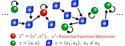
Figure 12: Image of Markov process $\{P^{0}\}$

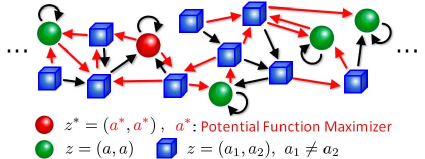
Figure 13: Image of Markov process $\{P^{\varepsilon}\}$ (Transitions colored by red can happen only when $\varepsilon\neq 0$)

In terms of the Markov process $\{P^{\varepsilon}\}$ induced by PHPIP, the following lemma holds.

Lemma 4

The Markov process $\{P^{\varepsilon}\}$ induced by PHPIP applied to the constrained strategic game $\Gamma$ in (9) with (8) is a regular perturbation of $\{P^{0}\}$ under Assumption 1.

Proof:

See Appendix A ∎

From Lemma 4, the perturbed process $\{P^{\varepsilon}\}$ is irreducible and aperiodic, and hence there exists a unique stationary distribution $\mu(\varepsilon)$ for every $\varepsilon$. We also see from the former half of Lemma 3 that $\lim_{\varepsilon\rightarrow 0+}\mu(\varepsilon)$ exists and the limiting distribution is the stationary distribution of $\{P^{0}\}$.

We also have the following lemma.

Lemma 5

Consider the Markov process $\{P^{\varepsilon}\}$ induced by PHPIP applied to the constrained strategic game $\Gamma$ in (9) with (8). Then, the recurrent communication classes of the unperturbed Markov process $\{P^{0}\}$ are given by elements of ${\rm diag}({\mathcal{A}})=\{(a,a)\in{\mathcal{A}}\times{\mathcal{A}}|\ a\in{\mathcal{A}}\}$, namely

$$H_{\iota}=\{(a^{\iota},a^{\iota})\},\ \iota=1,\cdots,|{\mathcal{A}}|.$$ (19)

Proof:

See Appendix B. ∎

The lemma means that all the paths over the Markov process $\{P^{0}\}$ eventually reach and remain at a state such that $a(k-1)=a(k)$ as illustrated in Fig. 13. Meanwhile, the process $\{P^{\varepsilon}\},\ \varepsilon\neq 0$ contains paths traversing two of such states as in Fig. 13.

We next introduce the following terminology, where we use the notation

$${\mathcal{E}}_{s}:=\{(z=(a,a),z^{\prime}=(a^{\prime},a^{\prime}))\in{\rm diag}({\mathcal{A}})\times{\rm diag}({\mathcal{A}})|\$$

$$\hskip 85.35826pt\exists v_{i}\in{\mathcal{V}}\mbox{ s.t. }a_{i}\in{\mathcal{C}}_{i}(a_{i}^{\prime}),a_{i}\neq a_{i}^{\prime}\mbox{ and }a_{-i}=a_{-i}^{\prime}\}.$$ (20)

Definition 5 (Straight Route)

A feasible path over $\{P^{\varepsilon}\}$ from $z^{1}=(a^{1},a^{1})$ to $z^{2}=(a^{2},a^{2})$ such that $(z^{1},z^{2})\in{\mathcal{E}}_{s}$ is said to be a straight route if the path describes the two rounds transitions that only $v_{i}$ satisfying $a^{1}_{i}\neq a^{2}_{i}$ chooses $a_{i}(k+1)=a_{i}^{2}$ through exploration at the first round and he also chooses $a_{i}(k+2)=a_{i}^{2}$ at the second round while the other sensors do not update their actions (Fig. 14). In addition, a feasible path over $\{P^{\varepsilon}\}$ from $z^{1}\in{\rm diag}({\mathcal{A}})$ to $z^{2}\in{\rm diag}({\mathcal{A}})$ is said to be an $M$-straight-route if the path contains $M$ nodes in ${\rm diag}({\mathcal{A}})$ including $z^{1}$ and $z^{2}$, visits the $M$ nodes only once, and any path between such nodes are straight routes.

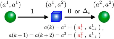
Figure 14: Straight route (the numbers above the arrows describe resistances of transitions)

In terms of the straight route, we have the following lemmas.

Lemma 6

Consider paths from any state $z^{1}=(a^{1},a^{1})\in{\rm diag}({\mathcal{A}})$ to any state $z^{2}=(a^{2},a^{2})\in{\rm diag}({\mathcal{A}})$ such that $(z^{1},z^{2})\in{\mathcal{E}}_{s}$ over the process $\{P^{\varepsilon}\}$ induced by PHPIP applied to the game $\Gamma$ in (9) with (8). Then, under Assumption 3, the resistance $\chi(\rho)$ of the straight route $\rho$ from $z^{1}$ to $z^{2}$ is strictly smaller than $3/2$ and $\chi(\rho)$ is minimal among all paths from $z^{1}$ to $z^{2}$.

Proof:

See Appendix C. ∎

Lemma 7

Consider the Markov process $\{P^{\varepsilon}\}$ induced by PHPIP applied to the game $\Gamma$ in (9) with (8). Let us describe an $M$-straight-route $\rho$ from state $z^{1}=(a^{1},a^{1})$ to state $z^{2}=(a^{2},a^{2})$ as $\rho:\ z^{(1)}=z^{1}{\Rightarrow}z^{(2)}{\Rightarrow}\cdots\Rightarrow z^{(M-1)}{\Rightarrow}z^{(M)}=z^{2}$, where $z^{(l)}=(a^{(l)},a^{(l)})\in{\rm diag}({\mathcal{A}}),l\in\{1,\cdots,M\}$ and all the arrows between them are straight routes. In addition, we consider the (reverse) $M$-straight-route $\rho^{\prime}:\ z^{(1)}=z^{1}{\Leftarrow}z^{(2)}{\Leftarrow}\cdots{\Leftarrow}z^{(M-1)}{\Leftarrow}z^{(M)}=z^{2}$ from $z^{2}$ to $z^{1}$. Then, under Assumption 3, if $\phi(a^{0})>\phi(a^{1})$, the inequality $\chi(\rho)>\chi(\rho^{\prime})$ holds true.

Proof:

See Appendix D. ∎

V-C Proof of Theorems

Proof of Theorem 1

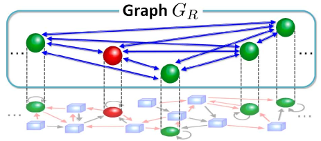
Figure 15: Graph $G_{R}$

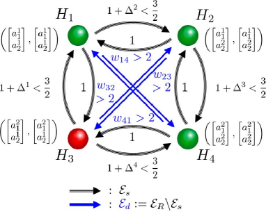
Figure 16: Illustrative example of a two player game

Let us form the directed graph $G_{R}=({\mathcal{H}},{\mathcal{E}}_{R},{\mathcal{W}}_{R})$ as in Subsection V-A over the recurrent communication classes for the unperturbed Markov process $\{P^{0}\}$ induced by PHPIP (Fig. 16). From (19), the node set ${\mathcal{H}}$ of the graph $G_{R}$ is given by ${\rm diag}({\mathcal{A}})$. Since all the recurrent communication classes have only one element from (19), the weight of the edge for any two states $z^{1}$ and $z^{2}\in{\rm diag}({\mathcal{A}})$ is simply given by the path with the minimal resistance among all paths from $z^{1}$ to $z^{2}$ over $\{P^{\varepsilon}\}$. In addition, Lemma 3 proves that if $(z^{1},z^{2})\in{\mathcal{E}}_{s}$ defined by (20), the minimal weight is given by the straight route from $z^{1}$ to $z^{2}$. For instance, let us consider a two player game with ${\mathcal{A}}_{1}=\{a_{1}^{1},a_{1}^{2}\}$ and ${\mathcal{A}}_{2}=\{a_{2}^{1},a_{2}^{2}\}$. Then, graph $G_{R}$ is illustrated as in Fig. 16, where only the edges colored by blue are contained in ${\mathcal{E}}_{d}:={\mathcal{E}}_{R}\setminus{\mathcal{E}}_{s}$ and have resistance greater than 2 since both of two players have to take exploration to escape from the state.

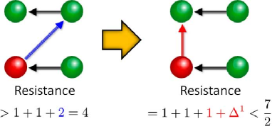
Figure 17: Trees with root $H_{1}$ over graph in Fig. 16

Figure 18: Resistance trees (the red node is the state $z^{*}=(a^{*},a^{*})$ with the potential function maximizer $a^{*}$)

Let us focus on $l$-trees over $G_{R}$ with a root $H_{l}=z^{l}\in{\rm diag}({\mathcal{A}})$. Recall now that the resistance of the tree is the sum of the weights of all edges constituting the tree as defined in Subsection V-A. Let us now consider a tree for the graph in Fig. 16 containing an edge in ${\mathcal{E}}_{d}$ (Left figure of Fig. 18). Then, it is easy to confirm that a tree with a smaller resistance can be formed by replacing the edge in ${\mathcal{E}}_{d}$ by an edge in ${\mathcal{E}}_{s}$ as illustrated in the right figure of Fig. 18. From this example, we have a conjecture that the minimal resistance tree consists only of edges in ${\mathcal{E}}_{s}$. The following lemma proves that the conjecture is true for a general case with $n$ sensors.

Lemma 8

Consider the weighted directed graph $G_{R}$ constituted from the Markov process $\{P^{\varepsilon}\}$ induced by PHPIP applied to the constrained strategic game $\Gamma$ in (9) with (8). Let us denote by ${\mathcal{T}}=({\rm diag}({\mathcal{A}}),{\mathcal{E}}_{l},{\mathcal{W}}_{l})$ the minimal resistance tree with root $z^{l}\in{\rm diag}({\mathcal{A}})$. If Assumptions 1 and 3 are satisfied, then the edge set ${\mathcal{E}}_{l}$ must be a subset of ${\mathcal{E}}_{s}$.

Proof:

See Appendix E. ∎

We are ready to prove Theorem 1. It is now sufficient to prove that all the stochastically stable states of $\{P^{\varepsilon}\}$ are included in ${\rm diag}(\arg\max_{a\in{\mathcal{A}}}\phi(a))$, since the probability of $a(k)\in\arg\max_{a\in{\mathcal{A}}}\phi(a)$ is greater than the probability of $z(k)=(a(k-1),a(k))\in{\rm diag}(\arg\max_{a\in{\mathcal{A}}}\phi(a))$. We also see from (19) and Lemmas 3 and 4 that we need only to prove that the states in ${\rm diag}({\mathcal{A}})$ with the minimal stochastic potential are included in $\arg\max_{a\in{\mathcal{A}}}\phi(a)$.

We first introduce the notations $z^{\prime}=(a^{\prime},a^{\prime})\in{\rm diag}({\mathcal{A}})$ with $a^{\prime}\notin\arg\max_{a\in{\mathcal{A}}}\phi(a)$ and $z^{*}=(a^{*},a^{*})\in{\rm diag}({\mathcal{A}})$ with $a^{*}\in\arg\max_{a\in{\mathcal{A}}}\phi(a)$. Let the minimal resistance tree for the state $z^{\prime}$ be denoted by $T$. Then, there exists a unique path $\rho$ from $z^{*}$ to $z^{\prime}$ over $T$. From Lemma 8, the path $\rho$ corresponds to an $M$-straight-route for some $M$. Now, we can build a tree $T^{\prime}$ with root $z^{*}$ such that only the path $\rho$ is replaced by its reverse path $\rho^{\prime}$ (Fig. 18). Then, we have $\chi(\rho)>\chi(\rho^{\prime})$ from Lemma 7 since $\phi(a^{*})>\phi(a^{\prime})$. Thus, the resistance of $T^{\prime}$ is smaller than that of $T$ and the stochastic potential of $z^{*}$ is smaller than or equal to the resistance of $T^{\prime}$. The statement holds regardless of the selection of $a^{\prime}$. This completes the proof.

Proof of Theorem 2

Let us next consider PIPIP with time-varying $\varepsilon(k)$ and first prove strong ergodicity of the inhomogeneous Markov process $\{P_{k}^{\varepsilon}\}$ induced by PIPIP. Here, a Markov process $\{P_{k}\}$ over a state space ${\mathcal{X}}$ is said to be strongly ergodic [31] if there exists a stochastic vector $\mu^{*}$ such that the following equation holds for any distribution $\mu$ on ${\mathcal{X}}$ and time $k_{0}$.

$${\rm lim}_{k\rightarrow\infty}\mu P(k_{0},k)=\mu^{*},\ P(k_{0},k):=\prod^{k-1}_{k^{\prime}=k_{0}}P_{k^{\prime}},\ 0\leq k_{0}<k.$$ (21)

If $\{P_{k}\}$ is strongly ergodic, the distribution $\mu$ converges to the unique distribution $\mu^{*}$ from any initial state. Meanwhile, the process $\{P_{k}\}$ is said to be weakly ergodic [31] if the following equation holds for all ${x^{1}},x^{2},x^{3}\in{\mathcal{X}}$ and ${k_{0}}\in{\mathbb{Z}}_{+}$.

$$\lim_{k\rightarrow\infty}(P_{x^{1}x^{3}}(k_{0},k)-P_{x^{2}x^{3}}(k_{0},k))=0$$

Here, we also use the following lemmas.

Lemma 9

[31] A Markov process $\{P_{k}\}$ is strongly ergodic if the following conditions hold: (B1) The Markov process $\{P_{k}\}$ is weakly ergodic. (B2) For each $k$, there exists a stochastic vector $\mu^{k}$ on ${\mathcal{X}}$ such that $\mu^{k}$ is the left eigenvector of the transition matrix $P(k)$ with eigenvalue 1. (B3) The eigenvector $\mu^{k}$ in (B2) satisfies $\sum^{\infty}_{k=0}\sum_{x\in{\mathcal{X}}}|\mu^{k}_{x}-\mu^{k+1}_{x}|<\infty$. Moreover, if $\mu^{*}=\lim_{k\rightarrow\infty}\mu^{t}$, then $\mu^{*}$ is the vector in (21).

Lemma 10

[31] A Markov process $\{P_{k}\}$ is weakly ergodic if and only if there is a strongly increasing sequence of positive numbers $k_{\iota},\ \iota\in{\mathbb{Z}}_{+}$ such that

$$\sum_{\iota=0}^{\infty}\min_{x^{1},x^{2}\in{\mathcal{X}}}\sum_{x\in{\mathcal{B}}}\min\{P_{x^{1}x}(k_{\iota},k_{\iota+1}),P_{x^{2}x}(k_{\iota},k_{\iota+1})\}=\infty$$

We next prove strong ergodicity of $\{P_{k}^{\varepsilon}\}$. Conditions (B2), (B3) in Lemma 9 can be proved in the same way as [14]. We thus mention only Condition (B1). Recall now that the probability of transition $z^{1}\rightarrow z^{2}$ is given by (24). Since $\varepsilon(k)$ is strictly decreasing, there is $k_{0}\geq 1$ such that $k_{0}$ is the first round satisfying

$$(1-\varepsilon(k))(1-\kappa\varepsilon(k)^{\Delta_{i}})\geq\frac{\varepsilon(k)}{C-1},\ 1-\varepsilon(k)\geq\frac{\varepsilon(k)^{(1-\Delta_{i})}}{\kappa(C-1)}.$$ (22)

The existence of $\varepsilon$ satisfying (22) is guaranteed by (14). For all $k\geq k_{0}$, we have

$$P_{z^{1}z^{2}}^{\varepsilon}(k)\geq\left(\frac{\varepsilon(k)}{C-1}\right)^{n}.$$

We next define $x_{z}=\arg\min_{x\in{\mathcal{B}}}P_{xz}(k,k+D+1)$ for any $z\in{\mathcal{B}}$. Then, similarly to [14],

$$\min_{z^{0}\in{\mathcal{B}}}P_{z^{0}z}(k,k+D+1)\geq P^{\varepsilon(k)}_{x_{z}z^{1}}\cdots P^{\varepsilon(k+D-1)}_{z^{D-1}z^{D}}P^{\varepsilon(k+D)}_{z^{D}z}\geq\Big{(}\frac{\varepsilon(k)}{C-1}\Big{)}^{n(D+1)}.$$

Following [14] again, we have the following inequality with $k_{\iota}=(D+1)\iota$ and $(D+1)\iota_{0}\geq k_{0}$.

$$\sum_{\iota=0}^{\infty}\min_{z^{1},z^{2}\in{\mathcal{B}}}\sum_{z\in{\mathcal{B}}}\min\{P_{z^{1}z}(k_{\iota},k_{\iota+1}),P_{z^{2},z}(k_{\iota},k_{\iota+1})\}\geq|{\mathcal{B}}|\sum_{\iota=\iota_{0}}^{\infty}\Big{(}\frac{\varepsilon(k)}{C-1}\Big{)}^{n(D+1)}$$

$$=\frac{|{\mathcal{B}}|}{(C-1)^{(D+1)n}}\sum_{\iota=\iota_{0}}^{\infty}\frac{1}{(D+1)\iota}=\infty$$

This inequality and Lemma 10 prove (B1) and hence strong ergodicity of $\{P_{k}^{\varepsilon}\}$. Thus, the distribution $\mu(\varepsilon(k))$ converges to the unique distribution $\mu^{*}$ from any initial state. In addition, we also have $\mu^{*}=\mu(0)={\lim}_{\varepsilon\rightarrow 0}\mu(\varepsilon)$ from ${\lim}_{k\rightarrow\infty}\varepsilon(k)=0$. We have already proved in Theorem 1 that any state $z$ satisfying $\mu_{z}(0)>0$ must be included in ${\rm diag}(\arg\max_{a\in{\mathcal{A}}}\phi(a))$. Hence, (15) holds and the proof of Theorem 2 is completed.

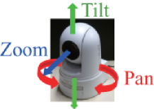
Figure 19: PTZ network camera

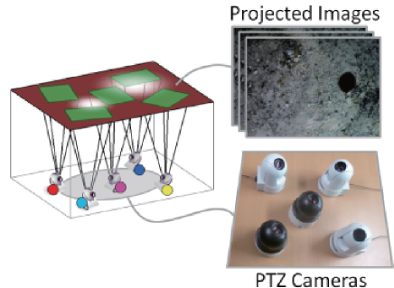
Figure 20: Overview of scenario

VI Experimental Case Study

We finally demonstrate the effectiveness of the presented approach through experiments on a testbed of PTZ visual sensor networks consisting of 5 PTZ cameras ${\mathcal{V}}=\{v_{1},v_{2},v_{3},v_{4},v_{5}\}$ (Fig. 20), where two of them ($v_{1}$ and $v_{2}$) are IPELA SNC-EP520 (SONY Corp.) and the other three ($v_{3}$, $v_{4}$ and $v_{5}$) are IPELA SNC-RZ25N (SONY Corp.). Note that the size of the acquired images is $640\times 480$ ($S_{i}\approx 3.0\times 10^{5}$) for every $v_{i}\in{\mathcal{V}}$. In this experiment, all the algorithms including image processing and the learning algorithm are run via Visual C++ (Microsoft Corp.).

Let the five cameras monitor a ceiling of a room on which an image is projected as illustrated in Fig. 20. Namely, we regard the ceiling as the environment and divide it into 130 squares ${\mathcal{R}}=\{r_{1},\cdots,r_{130}\}$, 10cm on a side. Note that sensors $v_{1},v_{2},v_{3},v_{4},v_{5}$ are respectively marked by purple, yellow, cyan, blue and red circles.

Figure 21: Sample image

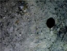
Figure 22: Projected image until 1500 round

Figure 23: Projected image after 1500 round

The action sets ${\mathcal{A}}_{i}=\varTheta_{i}\times\varPhi_{i}\times\varLambda_{i}$ are set as

$$\varTheta_{1}=\{(5/180)\pi n_{\theta}|\ n_{\theta}\in\{-34,-33,\cdots,34\}\},\$$

$$\varTheta_{i}=\{(5/180)\pi n_{\theta}|\ n_{\theta}\in\{-2,-1,\cdots,20\}\},\ i=2,3,4,5,$$

$$\varPhi_{i}=\{(5/180)\pi n_{\varphi}|\ n_{\varphi}\in\{15,16,\cdots,18\}\},\ i\in{\mathcal{V}},$$

$$\varLambda_{1}=\varLambda_{2}=\{6.8{\rm mm},13.6{\rm mm}\},\ \varLambda_{3}=\varLambda_{4}=\varLambda_{5}=\{8.2{\rm mm},16.4{\rm mm}\}.$$

Just to stabilize the evolution of the objective function, we introduce the constrained action sets

$$\bar{A}_{i}(a_{i})=\{(\theta_{i}^{\prime},\varphi_{i}^{\prime},\lambda_{i}^{\prime})|\ |\theta_{i}^{\prime}-\theta_{i}|\leq(5/180)\pi,\ |\varphi_{i}^{\prime}-\varphi_{i}|\leq(5/180)\pi,\ \lambda_{i}\in\varLambda_{i}\}$$

for all $a_{i}\in{\mathcal{A}}_{i}$ and $v_{i}\in{\mathcal{V}}$, which clearly satisfies Assumption 1.

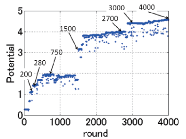
Figure 24: Evolution of global objective function

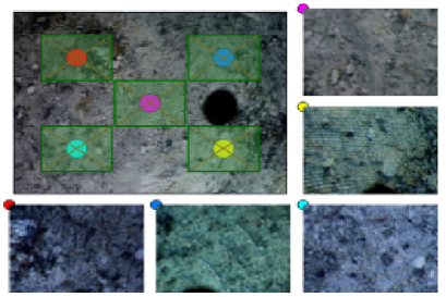
(a) Initial State

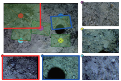
(b) 200 round

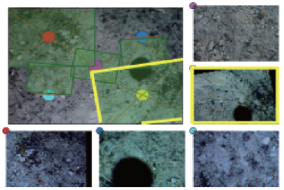
(c) 280 round

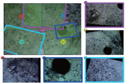
(d) 750 round

Figure 25: Snapshots of coverage area and acquired images for Fig. 23

The global objective function $W$ and utility function $U_{i}$ are selected as follows. Suppose that each sensor $v_{i}$ stores in memory a part of the sample image in Fig. 23 corresponding to each action in ${\mathcal{A}}_{i}$. Then, we employ (7) as $I^{\rm info}_{i,j}(a_{i})$. Since (7) inherently embodies the function of $I^{\rm qual}_{i,j}(a_{i})$, this experiment does not use $I^{\rm qual}_{i,j}(a_{i})$, and the function $\tilde{W}_{i,j}$ in (2) is chosen as

$$\tilde{W}_{i,j}=\left\{\begin{array}[]{ll}2I^{\rm info}_{i,j}(a_{i}),&\mbox{if }r_{j}\in{\mathcal{R}}_{i}(a_{i})\mbox{ and }2I^{\rm info}_{i,j}(a_{i})>\gamma\\ \gamma,&\mbox{if }r_{j}\in{\mathcal{R}}_{i}(a_{i})\mbox{ and }2I^{\rm info}_{i,j}(a_{i})\leq\gamma.\\ 0,&\mbox{if }r_{j}\not\in{\mathcal{R}}_{i}(a_{i})\end{array}\right..$$ (23)

The positive parameter $\gamma>0$ is introduced to place value of monitoring a region containing no useful information in preparation to future environmental changes. In this experiment, we set $\gamma=1.5\times 10^{-2}$. We next define $W_{j}$ and $W$ by (4) and (6), and then scale them so that Assumption 3 is satisfied. Such a scaling is possible since the maximal value of $W_{i,j}$ in (23) can be easily estimated. Finally, the utility function $U_{i}$ is designed according to (8).

In this experiment, we first project the image in Fig. 23 on the environment, which differs from the sample image in Fig. 23 in that a small hole appears. Then, we run the learning algorithm with $\varepsilon=0.015$ and $\kappa=0.120$ for 1500 rounds. Note that all the sensors initially choose zoom-in mode (the larger $\lambda_{i}$). After that, we change the image projected on the environment to the image in Fig. 23 with a larger hole, and leave the state for 2500 rounds. Due to the nature of the objective function, it is intuitively desirable that sensors capture the holes with high resolution while keeping the total coverage area as wide as possible.

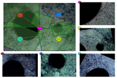
(a) 1500 round

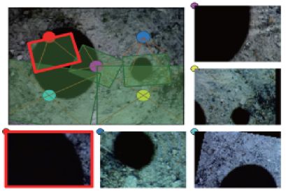
(b) 2700 round

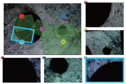
(c) 3000 round

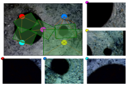
(d) 4000 round

Figure 26: Snapshots of coverage area and acquired images for Fig. 23

The experimental results are shown in Figs. 24, 25 and 26. Fig. 24 illustrates the evolution of the global objective function. We can confirm from this figure that the actions are basically selected so as to maximize the global objective function. Figs. 25 and 26 show the snapshots of the coverage area and the acquired images at the times marked on Fig. 24, where green boxes on the top left (large) pictures describe the field of views.

In Fig. 25(b), sensor $v_{5}$ (red) widely covers the environment by choosing zoom-out mode ($\lambda_{2}=6.8$mm) and $v_{4}$ (blue) captures the half of the hole, with zoom-in mode, which drive up the global objective function. We see from Fig. 25(c) that $v_{2}$ (yellow) covers the remaining half of the hole and also covers the unmonitored area, which also increases the objective function. Then, after a while, they reach a desirable configuration in Fig. 25(d), where the hole is monitored by a sensor in zoom-in mode and the remaining sensors achieve wide-ranging coverage by choosing zoom-out mode while avoiding overlaps of field of views.

Fig. 26(a) illustrates the configuration at the time when the image in Fig. 23 starts to be projected. We see from Fig. 26(b) that $v_{5}$ (red) monitors the hole in zoom-in mode, and from Fig. 26(c) that $v_{3}$ (cyan) also takes a similar action. Then, after the pan and tilt angles are finely tuned to avoid overlaps, they eventually reach the desirable configuration depicted in Fig. 26(d).

All the above results show the effectiveness of the present approach. Let us finally emphasize that the ideal results are achieved without using any prior information of environmental changes on when, where and how the changes occur.

VII Conclusions

In this paper, we have investigated a cooperative environmental monitoring for PTZ visual sensor networks and presented a distributed solution to the problem based on game theoretic cooperative control and payoff-based learning. We first have presented a novel optimal environmental monitoring problem. Then, after constituting a potential game via an existing utility design technique, we have presented a payoff-based learning algorithm based on [6] so that the vision sensors are led to not just a Nash equilibrium but the potential function maximizes. Finally, we have run experiments to demonstrate the effectiveness of the present approach.

The authors would like to thank Mr. S. Mori for his contributions in the experiments.

Appendix A Proof of Lemma 4

Condition (A2) in Definition 3 is straightforward from the structure of PHPIP. We thus prove only (A1) and (A3) below.

Consider a feasible transition $z^{1}\rightarrow z^{2}$ with $z^{1}=(a^{0},a^{1})\in{\mathcal{B}}$ and $z^{2}=(a^{1},a^{2})\in{\mathcal{B}}$, and partition the set of sensors ${\mathcal{V}}$ according to their behaviors along with the transition as

$$\Lambda_{1}\!\! \!\!=\!\! \!\!\{v_{i}\in{\mathcal{V}}|\ U_{i}(a^{1})\geq U_{i}(a^{0}),\ a^{2}_{i}\in{\mathcal{C}}_{i}(a_{i}^{1})\setminus\{a_{i}^{1}\}\},\ \Lambda_{2}=\{v_{i}\in{\mathcal{V}}|\ U_{i}(a^{1})\geq U_{i}(a^{0}),\ a^{2}_{i}=a_{i}^{1}\},$$

$$\Lambda_{3}\!\! \!\!=\!\! \!\!\{v_{i}\in{\mathcal{V}}|\ U_{i}(a^{1})<U_{i}(a^{0}),\ a^{2}_{i}\in{\mathcal{C}}_{i}(a_{i}^{1})\setminus\{a_{i}^{0},a_{i}^{1}\}\},$$

$$\Lambda_{4}\!\! \!\!=\!\! \!\!\{v_{i}\in{\mathcal{V}}|\ U_{i}(a^{1})<U_{i}(a^{0}),\ a^{2}_{i}=a_{i}^{1}\},\ \Lambda_{5}=\{v_{i}\in{\mathcal{V}}|\ U_{i}(a^{1})<U_{i}(a^{0}),\ a^{2}_{i}=a_{i}^{0}\}.$$

Then, the probability of transition $z^{1}\rightarrow z^{2}$ is described by

$$P_{z^{1}z^{2}}^{\varepsilon}=\prod_{i\in\Lambda_{1}}\frac{\varepsilon}{|{\mathcal{C}}_{i}(a_{i}^{1})|-1}\prod_{i\in\Lambda_{2}}(1-\varepsilon)\prod_{i\in\Lambda_{3}}\frac{\varepsilon}{|{\mathcal{C}}_{i}(a_{i}^{1})|-{\delta_{i}}}\prod_{i\in\Lambda_{4}}(1-\varepsilon)\kappa\varepsilon^{\Delta_{i}}\prod_{i\in\Lambda_{5}}(1-\varepsilon)(1-\kappa\varepsilon^{\Delta_{i}})$$ (24)

where $\delta_{i}=1$ if $a_{i}^{0}=a_{i}^{1}$ and $\delta_{i}=2$ otherwise. We see from (24) that the resistance $\chi(z^{1}\rightarrow z^{2})$ of transition $z^{1}\rightarrow z^{2}$ defined in (16) is equal to $|\Lambda_{1}|+|\Lambda_{3}|+\sum_{i\in\Lambda_{4}}\Delta_{i}$ since

$$0<\lim_{\varepsilon\rightarrow 0}\frac{P_{z^{1}z^{2}}^{\varepsilon}}{\varepsilon^{|\Lambda_{1}|+|\Lambda_{3}|+\sum_{i\in\Lambda_{4}}\Delta_{i}}}=\prod_{i\in\Lambda_{1}}\frac{1}{|{\mathcal{C}}_{i}(a_{i}^{1})|-1}\prod_{i\in\Lambda_{3}}\frac{1}{|{\mathcal{C}}_{i}(a_{i}^{1})|-h_{i}}\kappa^{|\Lambda_{4}|}<\infty$$ (25)

holds. Thus, (A3) in Definition 3 is satisfied.

Let us next check (A1) in Definition 3. From the rule of taking exploratory actions in Algorithm 1 and the second item of Assumption 1, we immediately see that the set of the states accessible from any $z\in{\mathcal{B}}$ is equal to ${\mathcal{B}}$. This implies that the perturbed Markov process $\{P^{\varepsilon}\}$ is irreducible. We next check aperiodicity of $\{P^{\varepsilon}\}$. It is clear that any state in ${\rm diag}({\mathcal{A}})$ has period 1. Let us next pick any $(a^{0},a^{1})$ from the set ${\mathcal{B}}\setminus{\rm diag}({\mathcal{A}})$. Since $a_{i}^{0}\in{\mathcal{C}}_{i}(a_{i}^{1})$ holds iff $a_{i}^{1}\in{\mathcal{C}}_{i}(a_{i}^{0})$ from Assumption 1, the following two paths are both feasible: $(a^{0},a^{1})\rightarrow(a^{1},a^{0})\rightarrow(a^{0},a^{1})$, $(a^{0},a^{1})\rightarrow(a^{1},a^{1})\rightarrow(a^{1},a^{0})\rightarrow(a^{0},a^{1})$. This implies that the period of state $(a^{0},a^{1})$ is $1$ and the process $\{P^{\varepsilon}\}$ is proved to be aperiodic. Hence the process $\{P^{\varepsilon}\}$ is both irreducible and aperiodic, which means (A1) in Definition 3.

Appendix B Proof of Lemma 5

Because of the rule at Step 2 of PHPIP, it is clear that any state belonging to ${\rm diag}({\mathcal{A}})$ cannot move to another state without explorations, which implies that all the states in ${\rm diag}({\mathcal{A}})$ itself form recurrent communication classes of the unperturbed Markov process $\{P^{0}\}$.

Let us consider the states in ${\mathcal{B}}\setminus{\rm diag}({\mathcal{A}})$ and prove that such states are never included in the recurrent communication classes of the unperturbed process $\{P^{0}\}$. Here, we use induction. We first consider $n=1$. If $U_{1}(a_{1}^{1})\geq U_{1}(a_{1}^{0})$, then the transition $(a_{1}^{0},a_{1}^{1})\rightarrow(a_{1}^{1},a_{1}^{1})$ is taken. Otherwise, a sequence of transitions $(a_{1}^{0},a_{1}^{1})\rightarrow(a_{1}^{1},a_{1}^{0})\rightarrow(a_{1}^{0},a_{1}^{0})$ occurs. Thus, for $n=1$, the state $(a_{1}^{0},a_{1}^{1})\in{\mathcal{B}}\setminus{\rm diag}({\mathcal{A}})$ is never included in recurrent communication classes of $\{P^{0}\}$.

We next make a hypothesis that there exists a $n^{\prime}\in{\mathbb{Z}}_{+}$ such that all the states in ${\mathcal{B}}\setminus{\rm diag}({\mathcal{A}})$ are not included in recurrent communication classes of the unperturbed Markov process $\{P^{0}\}$ for all $n\leq n^{\prime}$. Then, we consider the case $n=n^{\prime}+1$, where there are three possible cases:

(i)

$U_{i}(a^{1})\geq U_{i}(a^{0})\ {\forall i}\in{\mathcal{V}}=\{1,\cdots,n^{\prime}+1\}$,

(ii)

$U_{i}(a^{1})<U_{i}(a^{0})\ {\forall i}\in{\mathcal{V}}=\{1,\cdots,n^{\prime}+1\}$,

(iii)

$U_{i}(a^{1})\geq U_{i}(a^{0})$ for $n^{\prime\prime}$ agents where $n^{\prime\prime}\in\{2,\cdots,n^{\prime}\}$.

In case (i), the transition $(a^{0},a^{1})\rightarrow(a^{1},a^{1})$ must occur for $\varepsilon=0$ and, in case (ii), the transition $(a^{0},a^{1})\rightarrow(a^{1},a^{0})\rightarrow(a^{0},a^{0})$ should be selected. Thus, all the states in ${\mathcal{B}}\setminus{\rm diag}({\mathcal{A}})$ satisfying (i) or (ii) are never included in recurrent communication classes.

In case (iii), at the next iteration, all the agents $i$ satisfying $U_{i}(a^{1})\geq U_{i}(a^{0})$ choose the current action. Then, such agents possess a single action in the memory and, in case of $\varepsilon=0$, each agent has to choose either of the actions in the memory. Namely, these agents never change their actions in all subsequent iterations. The resulting situation is thus the same as the case of $n=n^{\prime}+1-n^{\prime\prime}$. From the above hypothesis, we can conclude that the states in case (iii) are also not included in recurrent communication classes. In summary, the states in ${\mathcal{B}}\setminus{\rm diag}({\mathcal{A}})$ are never included in the recurrent communication classes of $\{P^{0}\}$. The proof is thus completed.

Appendix C Proof of Lemma 6

Along with the straight route, the sensor $v_{i}$ such that $a^{1}_{i}\neq a^{2}_{i}$ first explores from $a_{i}^{1}$ to $a_{i}^{2}$, whose probability is $(1-\varepsilon)^{n-1}{\varepsilon}/{(|{\mathcal{C}}_{i}(a_{i}^{0})|-1)}$. This implies that the resistance of the transition $z^{1}=(a^{1},a^{1})\rightarrow(a^{1},a^{2})$ is equal to $1$.

We next consider the transition from $(a^{1},a^{2})$ to $z^{2}=(a^{2},a^{2})$. If $U_{i}(a^{2})\geq U_{i}(a^{1})$ is true, the probability of this transition is $(1-\varepsilon)^{n}$, whose resistance is equal to $0$. Otherwise, the inequality $U_{i}(a^{2})<U_{i}(a^{1})$ holds and the probability of this transition is equal to $(1-\varepsilon)^{n}\times\kappa\varepsilon^{\Delta_{i}}$, whose resistance is $\Delta_{i}$. See Fig. 14 for the graphic description of the above sentences. Let us now notice that the resistance $\chi(\rho)$ of the straight route $\rho$ is equal to the sum of the resistances of transitions $(a^{1},a^{1})\rightarrow(a^{1},a^{2})$ and $(a^{1},a^{2})\rightarrow(a^{2},a^{2})$ from (18), and that $\Delta_{i}<1/2$ from Assumption 3. Hence, we can conclude that $\chi(\rho)$ is smaller than $3/2$.

Let us next prove that the above resistance is minimal among all paths from $z^{1}$ to $z^{2}$. Suppose now that there is a path $\rho^{\prime}$ other than the straight route $\rho$ such that $\chi(\rho^{\prime})<\chi(\rho)<3/2$. Then, the path can accept only one exploration of one sensor since two explorations lead to resistance $2$. We see from Algorithm 1 that any sensor with $a_{i}(k-1)=a_{i}(k-2)$ would not take an action other than $a_{i}(k-1)$ without exploration regardless of the other sensors’ actions. Thus, the sensor taking exploration has to be $v_{i}$ such that $a_{i}^{1}\neq a_{i}^{2}$.

If we denote the chosen action through the exploration by $a_{i}^{\prime}$, then the available joint action in the future is limited to $a^{1}$ and $(a_{i}^{\prime},a^{1}_{-i})$ since no exploration will be taken. Thus, in order that $z^{2}$ will be chosen in the future, $a_{i}^{\prime}$ must be equal to $a_{i}^{2}$, and then either of $a^{1}$ and $a^{2}$ can occur afterward. Accordingly, the only way to reach $z^{2}$ at a round is to follow the transition $(a^{1},a^{2})\rightarrow(a^{2},a^{2})$, whose resistance is the same as $\chi(r)-1$. This contradicts the assumption of $\chi(\rho^{\prime})<\chi(\rho)$, and hence the proof is completed.

Appendix D Proof of Lemma 7

As shown in Appendix C, the resistance of a straight route must be equal to $1$ or $1+\Delta_{i}\in(1,3/2)$. Suppose now that the route $\rho$ contains $M_{\rho}$ straight routes with resistance greater than $1$, and $\rho^{\prime}$ contains $M_{\rho^{\prime}}$ such straight routes. Let us also denote by $v_{i_{\iota}}$ the sensor taking exploration along with the straight route $z^{(\iota)}\Rightarrow z^{(\iota+1)}$ in $\rho$. Then, the sensor $v_{i_{\iota}}$ also takes exploration along with $z^{(\iota)}\Leftarrow z^{(\iota+1)}$ in $\rho^{\prime}$. We also use the notations

$$\tilde{\Delta}_{{\iota}}:=U_{i_{\iota}}(a^{(\iota)})-U_{i_{\iota}}(a^{(\iota+1)}),\ \tilde{\Delta}^{\prime}_{{\iota}}:=-\tilde{\Delta}_{{\iota}}.$$

Since $z^{(\iota)}\Rightarrow z^{(\iota+1)}$ is a straight route and hence only $v_{i_{\iota}}$ changes his action along with the route, the following equation holds from Lemma 1 and (10).

$$\tilde{\Delta}_{{\iota}}=U_{i_{\iota}}(a^{(\iota)})-U_{i_{\iota}}(a^{(\iota+1)})=\phi(a^{(\iota)})-\phi(a^{(\iota+1)})$$ (26)

From the proof of Lemma 6, the resistance of $z^{(\iota)}\Rightarrow z^{(\iota+1)}$ in $\rho$ should satisfy

$$\chi(z^{(\iota)}\Rightarrow z^{(\iota+1)})=\left\{\begin{array}[]{ll}1,&\mbox{if }U_{i_{\iota}}(a^{(\iota+1)})\geq U_{i_{\iota}}(a^{(\iota)})\\ 1+\tilde{\Delta}_{{\iota}}\in(1,3/2),&\mbox{if }U_{i_{\iota}}(a^{(\iota+1)})<U_{i_{\iota}}(a^{(\iota)}),\end{array}\right.$$ (29)

while the resistance of $z^{(\iota)}\Leftarrow z^{(\iota+1)}$ in $\rho^{\prime}$ is given as

$$\chi(z^{(\iota)}\Leftarrow z^{(\iota+1)})=\left\{\begin{array}[]{ll}1+\tilde{\Delta}_{\iota}^{\prime}\in(1,3/2),&\mbox{if }U_{i_{\iota}}(a^{(\iota+1)})\geq U_{i_{\iota}}(a^{(\iota)})\\ 1,&\mbox{if }U_{i_{\iota}}(a^{(\iota+1)})<U_{i_{\iota}}(a^{(\iota)}).\end{array}\right.$$ (32)

Namely, either of the resistances of $z^{(\iota)}\Rightarrow z^{(\iota+1)}$ and $z^{(\iota+1)}\Leftarrow z^{(\iota)}$ is exactly $1$ and the other is greater than $1$ (Fig. 27) except for the case that $U_{i}(a^{(\iota+1)})=U_{i}(a^{(\iota)})$ in which the resistances are both equal to $1$. Let us now collect all the $\tilde{\Delta}_{{\iota}}$ such that the resistance of $z^{(\iota)}\Rightarrow z^{(\iota+1)}$ is greater than $1$ and number them as $\bar{\Delta}_{1},\cdots,\bar{\Delta}_{M_{\rho}}$. Similarly, we define $\bar{\Delta}^{\prime}_{1},\cdots,\bar{\Delta}^{\prime}_{M_{\rho^{\prime}}}$ for the reverse route $\rho^{\prime}$. Then, from (26), we obtain

$$\Delta_{1}+\cdots+\Delta_{M_{\rho}}-(\Delta^{\prime}_{1}+\cdots+\Delta^{\prime}_{M_{\rho^{\prime}}})=\phi(a^{1})-\phi(a^{2}).$$ (33)

Note that (33) holds even in the presence of pairs $(a^{(\iota)},a^{(\iota+1)})$ such that $U_{i_{\iota}}(a^{(\iota+1)})=U_{i_{\iota}}(a^{(\iota)})$. Since $\Delta_{1}+\cdots+\Delta_{M_{\rho}}=\chi(\rho)-(M-1)$ and $\Delta^{\prime}_{1}+\cdots+\Delta^{\prime}_{M_{\rho^{\prime}}}=\chi(\rho^{\prime})-(M-1)$ from (18), we obtain $\chi(\rho)=\chi(\rho^{\prime})+\phi(a^{0})-\phi(a^{1})$, which means the statement of this lemma.

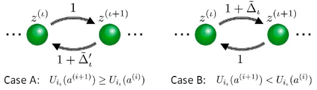
Figure 27: Resistance of a straight route (The numbers around arrows describe resistances of paths)

Appendix E Proof of Lemma 8

The edges of $G_{R}$, denoted by ${\mathcal{E}}_{R}$, are divided into ${\mathcal{E}}_{s}$ in (20) and ${\mathcal{E}}_{d}:={\mathcal{E}}_{R}\setminus{\mathcal{E}}_{s}$. From Lemma 6, the weights of the edges in ${\mathcal{E}}_{s}$ are smaller than $3/2$. We next consider the weights of an edge from $z^{1}=(a^{1},a^{1})\in{\rm diag}({\mathcal{A}})$ to $z^{2}=(a^{2},a^{2})\in{\rm diag}({\mathcal{A}})$ such that $(z^{1},z^{2})\in{\mathcal{E}}_{d}$. Then, there exist more than $2$ sensors such that $a^{1}_{i}\neq a^{2}_{i}$, or only one sensor $v_{i}$ such that $a^{1}_{i}\neq a^{2}_{i}$ satisfies $a^{2}_{i}\notin{\mathcal{C}}_{i}(a^{1}_{i})$. In both cases, at least two explorations must happen to reach $z^{2}$ and hence the resistance of any path in ${\mathcal{E}}_{d}$ has to be greater than $2$. Namely, we have

$$w_{l_{s}l_{s}^{\prime}}<w_{l_{d},l_{d}^{\prime}}\ \ {\forall}(H_{l_{s}},H_{l_{s}^{\prime}})\in{\mathcal{E}}_{s}\mbox{ and }(H_{l_{d}},H_{l_{d}^{\prime}})\in{\mathcal{E}}_{d}.$$ (34)

We next form a graph $G_{R}^{\prime}=({\mathcal{H}},{\mathcal{E}}_{R},W_{R}^{\prime})$ by just reversing the weights of all edges over graph $G_{R}$. Namely, the weight $w_{ll^{\prime}}$ on $G_{R}$ is equal to the weight $w_{l^{\prime}l}$ on $G_{R}^{\prime}$. Let us now apply the Chu-Liu/Edmonds Algorithm [33] to the graph $G_{R}^{\prime}$ and compute the minimal tree with a root $H_{R}$ such that there is a unique path from $H_{R}$ to any node (the directions of edges are opposite to the tree defined in Subsection V-A). Then, it is not difficult to confirm that reversing the directions of all edges of the minimal tree yields the minimal resistance tree with root $H_{R}$ over $G_{R}$. Hence, it is sufficient to prove that the Chu-Liu/Edmonds Algorithm provides a tree consisting only of edges in ${\mathcal{E}}_{s}$.

In the algorithm [33], every node in ${\mathcal{H}}\setminus\{H_{R}\}$ initially chooses the incoming edge with the minimal weight. Then, only edges in ${\mathcal{E}}_{s}$ can be chosen at the initial step from (34). If the resulting graph ${\mathcal{T}}_{0}$ consisting only of such edges is acyclic, then the minimum spanning tree is formed and the statement of this lemma is true. Otherwise, there is at least one cycle in ${\mathcal{T}}_{0}$.

We next focus on one of such cycles denoted by $G_{\rm cyc}=({\mathcal{H}}_{\rm cyc},{\mathcal{E}}_{\rm cyc},{\mathcal{W}}_{\rm cyc})$, where all edges in ${\mathcal{E}}_{\rm cyc}$ have to be contained in ${\mathcal{E}}_{s}$. In the following, the weight of the edge in ${\mathcal{E}}_{\rm cyc}$ entering a node $H_{l}\in{\mathcal{H}}_{\rm cyc}$ is denoted by $w_{\rm cyc}^{l}$, and we define $\bar{w}_{\rm cyc}:=\min_{H_{l}\in{\mathcal{H}}_{\rm cyc}}w_{\rm cyc}^{l}$. Then, each node $H_{l}$ in ${\mathcal{H}}_{\rm cyc}$ computes the temporal weights for all edges from $H_{l^{\prime}}\notin{\mathcal{H}}_{\rm cyc}$ to $H_{l}$ over $G_{R}^{\prime}$ by

$$\tilde{w}_{ll^{\prime}}=w^{\prime}_{ll^{\prime}}-w_{\rm cyc}^{l}+\bar{w}_{\rm cyc},$$ (35)

and identifies a node $H_{l^{\prime}}$ providing the minimal $\tilde{w}_{ll^{\prime}}$, where such a node $H_{l^{\prime}}$ is denoted by $\bar{H}_{l}$ and the corresponding $\tilde{w}_{ll^{\prime}}$ is denoted by $\bar{w}_{l}$. Then, we seek $H_{l^{*}}\in{\mathcal{H}}_{\rm cyc}$ with the minimal $\bar{w}_{l}$ and replace the edge entering $H_{l^{*}}$ over ${\mathcal{T}}_{0}$ by the edge $(H_{l^{*}},H_{l})$.

Chu-Liu/Edmonds Algorithm repeats the above process and eventually finds the minimum spanning tree. Namely, if we can prove that $(H_{l^{*}},H_{l})$ must be included in ${\mathcal{E}}_{s}$, the statement of the lemma is true. Now, notice that there exists at least one $H_{l}\in{\mathcal{H}}_{\rm cyc}$ such that the set

$${\mathcal{H}}_{l}=\{H_{l^{\prime}}\in{\mathcal{H}}\setminus{\mathcal{H}}_{\rm cyc}|\ (H_{l^{\prime}},H_{l})\in{\mathcal{E}}_{s}\}$$

is not empty from Assumption 1. For such a node $H_{l}$, the node $\bar{H}_{l}$ must be chosen from ${\mathcal{H}}_{l}$ since (34) holds and the second and third terms in (35) are common for all options of $H_{l^{\prime}}\notin{\mathcal{H}}_{\rm cyc}$. Then, $w^{\prime}_{ll^{\prime}}$ in (35) must be smaller than $3/2$ since $(H_{l^{\prime}},H_{l})\in{\mathcal{E}}_{s}$, and $-w_{\rm cyc}^{l}+\bar{w}_{\rm cyc}\in(-1/2,0]$ holds since $w_{\rm cyc}^{l}\in[1,3/2)$, $\bar{w}_{\rm cyc}\in[1,3/2)$, and $\bar{w}_{\rm cyc}:=\min_{H_{l}\in{\mathcal{H}}_{\rm cyc}}w_{\rm cyc}^{l}$. Namely, $\bar{w}_{l}$ must be smaller than $3/2$ for all $H_{l}$ such that ${\mathcal{H}}_{l}$ is not empty. In contrast, for any $H_{l}$ such that ${\mathcal{H}}_{l}$ is empty, $w^{\prime}_{ll^{\prime}}$ in (35) must be greater than or equal to $2$ because of $(H_{l},H_{l^{\prime}})\in{\mathcal{E}}_{d}$. Then, by using $-w_{\rm cyc}^{l}+\bar{w}_{\rm cyc}\in(-1/2,0]$ again, $\bar{w}_{l}$ is proved to be greater than $3/2$ and such $H_{l^{\prime}}$ is never selected as $H_{l^{*}}$. Namely, $(H_{l^{*}},H_{l})$ must be contained in ${\mathcal{E}}_{s}$. This completes the proof.

References

- [1] M. Dunbabin and L. Marques, “Robots for environmental monitoring: Significant advancements and applications,” IEEE Robotics & Automation Magazine, Vol. 19, No. 1, pp. 24–39, 2012.
- [2] A. K. Roy-chowdhury and B. Song, Camera networks: The acquisition and analysis of videos over wide areas, Morgan and Claypool Publishers, 2011.
- [3] J. R. Marden, G. Arslan and J. S. Shamma, “Cooperative control and potential games,” IEEE Transactions on Systems, Man and Cybernetics, Vol. 39, No. 6, pp. 1393–1407, 2009.
- [4] R. Gopalakrishnan, J. R. Marden and A. Wierman, “An architectural view of game theoretic control,” ACM SIGMETRICS Performance Evaluation Review, Vol. 38, No. 3, pp. 31–36, 2011.
- [5] J. R. Marden and J. S. Shamma, “Revisiting log-linear learning : Asynchrony, completeness and payoff-based implementation,” Games and Economic Behavior, Vol. 75, No. 2, pp. 788–808, 2012.
- [6] J. R. Marden, H. P. Young, G. Arslan and J. S. Shamma, “Payoff-based dynamics for multi-player weakly acyclic games,” SIAM Journal on Control and Optimization, Vol. 48, No. 1, pp. 373–396, 2009.
- [7] J. R. Marden, H. P. Young and L. Y. Pao, “Achieving Pareto optimality through distributed learning,” Proc. of the 51st IEEE Conference on Decision and Control, pp. 7419–7424, 2012.
- [8] T. Goto, T. Hatanaka and M. Fujita, “Payoff-based inhomogeneous partially irrational play for potential game theoretic cooperative control of multi-agent systems,” Proc. of 2012 American Control Conference, pp. 2380–2387, 2012.
- [9] B. Song, C. Ding, A. Kamal, J. A. Farrell and A. K. Roy-Chowdhury, “Distributed camera networks: integrated sensing and analysis for wide area scene understanding,” IEEE Signal Processing Magazine, Vol. 28, No. 3, pp. 20–31, 2011.
- [10] T. Hatanaka and M. Fujita, “Cooperative estimation of averaged 3D moving target object poses via networked visual motion observers,” IEEE Transactions on Automatic Control, Vol. 58, No. 3, to appear, 2013.
- [11] R. Tron and R. Vidal, “Challenges faced in deployment of camera sensor networks,” IEEE Signal Processing Magazine, Vol. 28, No. 3, pp. 32–45, 2011.
- [12] D. Borra, E. Lovisari, R. Carli, F. Fagnani and S. Zampieri, “Autonomous calibration algorithms for networks of cameras,” Proc. of 2012 American Control Conference, pp. 5126–5131, 2012.
- [13] C. Ding, B. Song, A. Morye, J. A. Farrell and A. K. Roy-Chowdhury, “Collaborative sensing in a distributed PTZ camera network,” IEEE Transactions on Image Processing, Vol. 21, No. 7, pp. 3282–3295, 2012.
- [14] M. Zhu and S. Martinez, “Distributed coverage games for energy-aware mobile sensor networks,” SIAM Journal on Control and Optimization, Vol. 51, No. 1, pp. 1–27, 2013.
- [15] M. Spindler, F. Pasqualetti and F. Bullo, “Distributed multi-camera synchronization for smart-intruder detection,” Proc. of 2012 American Control Conference, pp. 5120–5125, 2012.
- [16] C. G. Cassandras and W. Li, “Sensor networks and cooperative control,” European Journal of Control, Vol. 11, No. 4–5, pp. 436–463, 2005.
- [17] S. Martinez, J. Cortes, and F. Bullo, “Motion coordination with distributed information,” IEEE Control Systems Magazine, Vol. 27, No. 4, pp. 75–88, 2007.
- [18] C. H. Caicedo-N and M. Zefran, “A coverage algorithm for a class of non-convex regions,” Proc. of the 47th IEEE International Conference on Decision and Control, pp. 4244–4249, 2008.
- [19] J. Habibi, H. Mahboubi and A. G. Aghdam, “A nonlinear optimization approach to coverage problem in mobile sensor networks,” Proc. of the 50th IEEE Conference on Decision and Control, pp. 7255–7261, 2011.
- [20] Y. Wang and I. I. Hussein, “Awareness coverage control over large-scale domains with intermittent communications,” IEEE Transactions on Automatic Control, Vol. 55, No. 8, pp. 1850-1859, 2010.
- [21] M. S. Stankovic, K. H. Johansson and D. M. Stipanovic, “Distributed seeking of Nash equilibria with applications to mobile sensor networks,” IEEE Transactions on Automatic Control, Vol. 57, No. 4, pp. 904–919, 2012.
- [22] P. Hokayem, D. M. Stipanovic and M. Spong, “On persistent coverage control,” Proc. of the 46th IEEE Conference on Decision and Control, pp. 6130–6135, 2008.
- [23] N. Hubel CS. Hirche CA. Gusrialdi CT. Hatanaka CM. Fujita and O. Sawodny, “Coverage control with information decay in dynamic environments,” Proc. of the 17th IFAC World Congress, pp. 4180–4185, 2008
- [24] S. L. Smith, M. Schwager and D. Rus, “Persistent monitoring of changing environments using robots with limited range sensing,” Proc. of the IEEE International Conference on Robotics and Automation 2011, pp. 5448–5455, 2011.
- [25] C. G. Cassandras, X. Lin and X. C. Ding, “An optimal control approach to the multi-agent persistent monitoring problem,” Proc. of the 51st IEEE Conference on Decision and Control, pp. 2795-2800, 2012.
- [26] Y. Zhang, M. Rotea and N. Gans, “Sensors searching for interesting things: extremum seeking control on entropy maps,” Proc. of 50th IEEE Conference on Decision and Control and European Control Conference, pp. 4985–4991, 2011.
- [27] H. Takenaka, T. Y. Nakajima, A. Higurashi, A. Higuchi, T. Takamura, R. T. Pinker and T. Nakajima, “Estimation of solar radiation using a neural network based on radiative transfer,” Journal of Geophysical Research, Vol. 116, D08215, 2011.
- [28] M. S. Ghonima, B. Urquhart, C. W. Chow, J. E. Shields, A. Cazorla and J. Kleiss, “A method for cloud detection and opacity classification based on ground based sky imagery,” Atmospheric Measurement Techniques Discussions, Vol. 5, No. 4, pp. 4535–4569, 2012.
- [29] Y. Lim and J. S. Shamma, “Robustness of stochastic stability in game theoretic learning,” submitted for conference publication, 2012.
- [30] H. P. Young, Individual strategy and social structure: an evolutionary theory of institutions, Princeton University Press, 2001.
- [31] D. Isaacson and R. Madsen, Markov chains: theory and applications, New York, Wiley, 1976.
- [32] T. Goto, T. Hatanaka and M. Fujita, “Payoff-based inhomogeneous partially irrational play for potential game theoretic cooperative control of multi-agent systems,” downloadable at arXiv:1107.4838, 2011.
- [33] J. Edmonds, “Optimum branchings,” Journal of Research of the National Bureau of Standards, Vol. 71-B, pp. 233–240, 1967.