Hermitian four-well potential as a realization of a $\mathcal{PT}$-symmetric system

Abstract

A $\mathcal{PT}$-symmetric Bose-Einstein condensate can be theoretically described using a complex optical potential, however, the experimental realization of such an optical potential describing the coherent in- and outcoupling of particles is a nontrivial task. We propose an experiment for a quantum mechanical realization of a $\mathcal{PT}$-symmetric system, where the $\mathcal{PT}$-symmetric currents of a two-well system are implemented by coupling two additional wells to the system, which act as particle reservoirs. In terms of a simple four-mode model we derive conditions under which the two middle wells of the Hermitian four-well system behave exactly as the two wells of the $\mathcal{PT}$-symmetric system. We apply these conditions to calculate stationary solutions and oscillatory dynamics. By means of frozen Gaussian wave packets we relate the Gross-Pitaevskii equation to the four-mode model and give parameters required for the external potential, which provides approximate conditions for a realistic experimental setup.

In quantum mechanics an observable is described by an Hermitian operator. This is true in particular for the energy, which is represented by the Hamiltonian. The Hermicity is sufficient for purely real eigenvalues, but is this really a necessary condition? Bender and Boettcher found that for non-Hermitian Hamiltonians with a weaker condition, namely $\mathcal{PT}$ symmetry, there exist parameters for which the energy eigenvalue spectrum is purely real Bender98 , where $\mathcal{PT}$ stands for a combined action of parity $\mathcal{P}$ ($x\to-x$, $p\to-p$), and time reversal $\mathcal{T}$ ($x\to x$, $p\to-p$ with $\mathcal{T}\mathrm{i}=-\mathrm{i}\mathcal{T}$).

Due to the close analogy between the Schrödinger equation and the equations describing the propagation of light in structured wave guides, a $\mathcal{PT}$-symmetric optical system could be visualized Klaiman08 and experimentally investigated Guo09 ; Rueter10 . The necessary complex potential corresponds to a complex refractive index, which is realized by balanced gain and loss of light in the wave guide. Several other systems with $\mathcal{PT}$ symmetry have been suggested and partially realized, including lasers Chong11 ; Ge11 ; Liertzer12 , electronics Schindler11 ; Ramezani12 ; Schindler12 , microwave cavities Bittner12 , and quantum field theories Bender98 ; Bender12 . But up to date, a quantum mechanical realization of a $\mathcal{PT}$-symmetric system is still missing.

It was proposed Klaiman08 that a system similar to complex refractive indices in wave guides could be realized with Bose-Einstein condensates in double-well potentials, where particles are injected in one well and removed from the other one. BECs in $\mathcal{PT}$-symmetric double-well potentials have been investigated in the Bose-Hubbard model and the mean-field approximation Graefe08b ; Graefe08a ; Graefe10 ; Cartarius12b ; Cartarius12a . In these Refs., the $\mathcal{PT}$ symmetry is given by a complex potential which fulfills the condition $V^{*}(x)=V(-x)$ and describes the coherent in- and outcoupling of atoms into and from the system. It has already been shown that a bidirectional coupling between two BECs is possible and at the same time particles may be continuously ejected Shin05 ; Gati06 .

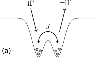
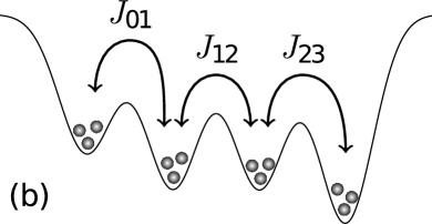
Figure 1: (a) $\mathcal{PT}$-symmetric two-well system with tunneling rate $J$ and complex potential $\pm\mathrm{i}\Gamma$, which describes coherent in- and outcoupling of atoms. (b) Alternatively, two additional wells serve as particle reservoirs and induce particle currents that – under application of specific system parameters to be determined – are equivalent to the $\mathcal{PT}$-symmetric currents of system (a).

In this letter we follow a different approach. Instead of injecting and removing particles, we couple two additional wells to a double-well system. The tunneling of the outer wells can be used to add and remove particles from the inner wells (see Fig. 1). We investigate, if just considering the two middle wells, they behave like the two wells of the $\mathcal{PT}$-symmetric two-well system. For the four-well potential we assume a combination of four Gaussian beams,

$$V_{\text{ext}}({\bm{r}})=\sum\limits_{i=0}^{3}V_{i}\exp\left[-\frac{2x^{2}}{w_{x}^{2}}-\frac{2y^{2}}{w_{y}^{2}}-\frac{2(z-s_{z}^{i})^{2}}{w_{z}^{2}}\right],$$ (1)

with $V_{i}<0$ the depth and $s_{z}^{i}$ the displacement along the $z$ axis of each well, and $w_{\alpha}$ the width of a single well in each direction. The dynamics of a BEC is described by the Gross-Pitaevskii equation (GPE)

$$\mathrm{i}\hbar\partial_{t}\psi({\bm{r}},t)=\left[-\frac{\hbar^{2}}{2m}\Delta+V_{\text{ext}}({\bm{r}})+Ng\left|\psi({\bm{r}},t)\right|^{2}\right]\psi({\bm{r}},t),$$ (2)

where $g=4\pi\hbar^{2}a_{\text{s}}/m$ is the strength of the nonlinearity, with $a_{\text{s}}$ being the scattering length.

It was shown that the $\mathcal{PT}$-symmetric two-mode model shows the features specific of $\mathcal{PT}$-symmetric systems Graefe12 . Therefore we use the simple, but instructive two- and four-mode models for our investigations. For the moment we neglect particle interaction, which will be taken into account later. The Hamiltonian of the linear, $\mathcal{PT}$-symmetric two-mode model is given by

$$H^{(2)}=\begin{pmatrix}\mathrm{i}\Gamma&-J\\ -J&-\mathrm{i}\Gamma\end{pmatrix},$$ (3)

which models a double-well system of non-interacting bosons. The real quantity $J>0$ designates the tunneling amplitude between the two wells, and $\Gamma\in\mathbb{R}$ gives the strength of the imaginary $\mathcal{PT}$-symmetric potential, which models gain and loss, respectively. Obviously, this Hamiltonian commutes with the combined action of parity and time reversal, $[\mathcal{PT},H^{(2)}]=0$, where the parity operator is given in this matrix representation by

$$\mathcal{P}=\begin{pmatrix}0&1\\ 1&0\end{pmatrix},$$ (4)

and time reversal is simply the complex conjugation. The eigenvalues and eigenvectors are easily found to be $E_{\pm}=\pm\sqrt{J^{2}-\Gamma^{2}}$ and $\psi_{\pm}=\left(\mathrm{i}\Gamma\pm\sqrt{J^{2}-\Gamma^{2}},-J\right)^{T}$ (unnormalized). For $\Gamma<J$ the eigenvalues are purely real and the eigenvectors obey $\mathcal{PT}$ symmetry. In the opposite case, $\Gamma>J$, the $\mathcal{PT}$ symmetry is broken and the eigenvalues become purely imaginary. Thus, the simple two-mode model features the basic properties of a $\mathcal{PT}$-symmetric Hamiltonian.

To gain deeper insight, and for an easier comparison with the later defined four-mode model, we give the time derivatives of the observables of the system. Two observables are the number of particles in each well, which are given by $n_{k}=\psi_{k}^{*}\psi_{k}$, where $\psi\in\mathbb{C}^{2}$ describes a quantum mechanical state. With the particle current $j_{12}=\mathrm{i}J\left(\psi_{1}\psi_{2}^{*}-\psi_{1}^{*}\psi_{2}\right)$ between the two wells the time-scaled ($t\to\hbar t$) Schrödinger equation can be brought to the closed set of differential equations for the observables

$$\partial_{t}n_{1}=-j_{12}+2\Gamma n_{1},\quad\quad\partial_{t}n_{2}=+j_{12}-2\Gamma n_{2},$$ (5a)

$$\partial_{t}j_{12}=2J^{2}(n_{1}-n_{2}).$$ (5b)

The imaginary potential induces particle currents from and to the environment, $j_{e1}=2\Gamma n_{1}$ and $j_{2e}=2\Gamma n_{2}$, both of which are proportional to the number of particles in the corresponding well.

It is now our main purpose to investigate, whether the behavior of the $\mathcal{PT}$-symmetric two-mode model (3) can be described by a Hermitian four-mode model, where two additional wells are coupled to the system. The Hamiltonian of the four-mode model is given by

$$H^{(4)}(t)=\begin{pmatrix}E_{0}(t)&-J_{01}(t)&0&0\\ -J_{01}(t)&0&-J_{12}&0\\ 0&-J_{12}&0&-J_{23}(t)\\ 0&0&-J_{23}(t)&E_{3}(t)\end{pmatrix}.$$ (6)

The two middle wells will be symmetric, hence $E_{1}=E_{2}=0$. The tunneling amplitudes and on-site energies of the outer wells are $J_{01}$, $J_{23}$, and $E_{0}$, $E_{3}$, respectively. They may be time-dependent, as denoted by the explicit time-dependence in Eq. (6). To be able to compare the four-mode model with the two-mode model, we calculate the time derivatives of the particle populations, which yields the simple relations

$$\partial_{t}n_{0} =-j_{01}, \partial_{t}n_{1} =j_{01}-j_{12},$$

$$\partial_{t}n_{2} =j_{12}-j_{23}, \partial_{t}n_{3} =j_{23},$$ (7)

where

$$j_{kl}=\mathrm{i}J_{kl}\left(\psi_{k}\psi_{l}^{*}-\psi_{k}^{*}\psi_{l}\right)$$ (8)

is the particle current between adjacent wells. By additionally considering the time derivative of $j_{12}$, we obtain

$$\partial_{t}n_{1}=j_{01}-j_{12},\quad\quad\partial_{t}n_{2}=j_{12}-j_{23},$$ (9a)

$$\partial_{t}j_{12}=2J_{12}^{2}\left(n_{2}-n_{1}\right)+J_{12}\left(J_{23}C_{13}-J_{01}C_{02}\right),$$ (9b)

where we defined $C_{kl}=\psi_{k}\psi_{l}^{*}+\psi_{k}^{*}\psi_{l}$. Comparing Eqs. (5) and (9) we can conclude that if the conditions

$$j_{01} =2\Gamma n_{1}, j_{23} =2\Gamma n_{2}, J_{01}C_{02} =J_{23}C_{13}$$ (10)

are fulfilled, the two middle wells of the Hermitian four-mode model (6) behave exactly as the two wells of the $\mathcal{PT}$-symmetric two-mode system (3).

We now need to give the explicit time-dependency of the free parameters of the Hamiltonian (6), $E_{0}$, $E_{3}$, $J_{01}$ and $J_{23}$, such that Eqs. (10) are fulfilled. For the tunneling elements we can set

$$J_{01}=dC_{13}, J_{23}=dC_{02},$$ (11)

where $d$ is a time-independent parameter, and can be tuned to bring the tunneling elements into an experimentally realizable range. The currents $j_{01}$ and $j_{23}$ have to fulfill Eqs. (10). However, with the tunneling elements determined by Eqs. (11), there are no free parameters left to adjust these currents. Instead, we take the time derivatives of Eqs. (10), which yields

$$\partial_{t}j_{01} =2\dot{\Gamma}n_{1}+2\Gamma\dot{n}_{1}=2\dot{\Gamma}n_{1}+2\Gamma\left(2\Gamma n_{1}-j_{12}\right),$$ (12a)

$$\partial_{t}j_{23} =2\dot{\Gamma}n_{2}+2\Gamma\dot{n}_{2}=2\dot{\Gamma}n_{2}+2\Gamma\left(j_{12}-2\Gamma n_{2}\right).$$ (12b)

where we allow the parameter $\Gamma$ to be explicitly time-dependent. For the last equalities we used Eqs. (Hermitian four-well potential as a realization of a $\mathcal{PT}$-symmetric system) and (10). Here, $\Gamma$ is not a quantity entering the Hamiltonian directly as in the two-mode model (3), but a free parameter, which determines the matrix elements of the Hamiltonian (6).

Now we can calculate the time derivatives of $j_{01}$ and $j_{23}$ from the definition (8). This leads to the linear system of equations for the on-site energies $E_{0}$ and $E_{3}$,

$$\begin{pmatrix}J_{01}C_{01}&d\tilde{j}_{01}\tilde{j}_{13}\\ -d\tilde{j}_{02}\tilde{j}_{23}&-J_{23}C_{23}\end{pmatrix}\begin{pmatrix}E_{0}\\ E_{3}\end{pmatrix}=\begin{pmatrix}v_{0}\\ v_{3}\end{pmatrix},$$ (13)

with the entries

$$v_{0}=2\dot{\Gamma}n_{1}+2\Gamma\left(j_{01}-j_{12}\right)-2J_{01}^{2}\left(n_{0}-n_{1}\right)$$

$$-J_{01}J_{12}C_{02}-d\left(J_{01}\tilde{j}_{03}+J_{12}\tilde{j}_{23}-J_{23}\tilde{j}_{12}\right)\tilde{j}_{01},$$ (14a)

$$v_{3}=2\dot{\Gamma}n_{2}+2\Gamma\left(j_{12}-j_{23}\right)-2J_{23}^{2}\left(n_{2}-n_{3}\right)$$

$$+J_{23}J_{12}C_{13}-d\left(J_{01}\tilde{j}_{12}-J_{12}\tilde{j}_{01}-J_{23}\tilde{j}_{03}\right)\tilde{j}_{23}.$$ (14b)

Here we have defined the modified currents $\tilde{j}_{kl}=\mathrm{i}\left(\psi_{k}\psi_{l}^{*}-\psi_{k}^{*}\psi_{l}\right)$. Thus, the on-site energies $E_{0}$ and $E_{3}$ are used to maintain the validity of Eqs. (10). Since the energies do not determine the currents but their time derivatives, the initial wave function must be chosen in such a way that the conditions are fulfilled.

So far we could find the explicit time-dependences of the matrix elements $E_{0}(t)$, $E_{3}(t)$, $J_{01}(t)$, and $J_{23}(t)$ of the four-mode model in order that at every time the two middle wells have the same behavior as the $\mathcal{PT}$-symmetric two-mode model. Thus our method is a valid possibility to realize a $\mathcal{PT}$-symmetric quantum mechanical system. To calculate the matrix elements at every time step we integrate the four-dimensional complex Schrödinger equation with a numerical integrator and use Eqs. (11) and (13). We now give two examples for different solutions.

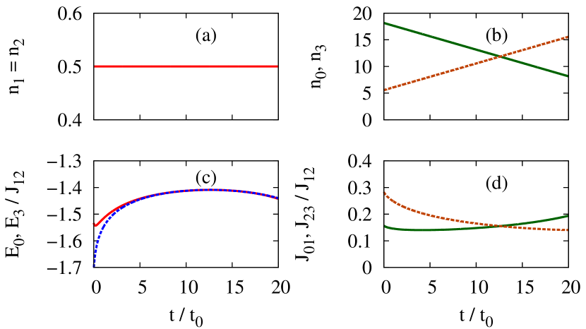
Figure 2: (Color online) (a) Populations $n_{1}=n_{2}=1/2$ of the middle wells, which are both equal and constant in time. (b) Populations $n_{0}$ (solid) and $n_{3}$ (dashed) of the outer wells, which depend linearly on the time, i. e. $\dot{n}_{0}=-\Gamma$ and $\dot{n}_{3}=\Gamma$. (c) Time-dependent on-site energies $E_{0}$ (solid) and $E_{3}$ (dashed). (d) Tunneling amplitudes $J_{01}$ (solid) and $J_{23}$ (dashed). Time is given in units of $t_{0}=\hbar/J_{12}$.

First we consider a quasi-stationary solution, i. e. a state in which the particle numbers in the two middle wells are stationary. These states correspond to the stationary solution of the two-mode model. We prepared this stationary solution for $\Gamma/J_{12}=0.5$ at $t=0$. Fig. 2 shows the results. As required, the number of particles in the middle wells are equal and constant in time (we have chosen the normalization such that $n_{1}+n_{2}=1$). From Eqs. (Hermitian four-well potential as a realization of a $\mathcal{PT}$-symmetric system) and (10) we then obtain $\dot{n}_{0}=-\Gamma$ and $\dot{n}_{3}=\Gamma$, plotted in Fig. 2(b). Figs. 2(c) and (d) show the calculated matrix elements. All of them vary only slightly in time. Due to the linear decrease of the number of particles in well 3 the available time for the $\mathcal{PT}$ symmetry is limited.

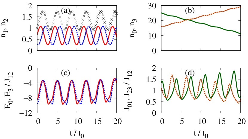
Figure 3: (Color online) Same as Fig. 2, but for oscillatory dynamics. Additionally, the total number of particles in wells 1 and 2 are plotted as black crosses in (a).

As a second example we prepared a non-stationary solution at $t=0$ for $\Gamma/J_{12}=0.5$ (Fig. 3). There are the typical Rabi-type oscillations, but with a smaller phase difference $\Delta\phi<\pi$, which leads to a non-constant added number of particles in the two middle wells. This value oscillates harmonically around its mean value. The same behavior is obtained for the optical system in Ref. Klaiman08 . The matrix elements show a quasi-oscillatory behavior. As before, the time for an exact $\mathcal{PT}$ symmetry is limited.

For these calculations, the initial conditions had to be chosen appropriately so that they obey $\mathcal{PT}$ symmetry. This would be a difficult task in an experiment. For that, we propose an approach of adiabatically increasing the $\mathcal{PT}$ parameter $\Gamma$. We start at the ground state of the four-well system, and increase $\Gamma$ according to $\Gamma(t)=\Gamma_{\text{f}}\left[1-\cos\left(\pi t/t_{\text{f}}\right)\right]/2$ for $t\in[0,t_{\text{f}}]$ (see Fig. 4a)). The quantities $\Gamma_{\text{f}}$ and $t_{\text{f}}$ have to be chosen such that $\dot{\Gamma}/\Gamma\ll\omega$, where $\omega$ is the typical oscillation frequency. The system then changes adiabatically from the ground state of the Hermitian system to a $\mathcal{PT}$-symmetric ground state.

So far we have neglected the contact interaction of the atoms. However, as we show next, taking into account the nonlinear contact interaction will not change the characteristic $\mathcal{PT}$-symmetric behavior. The Hamiltonian, which is nonlinear in the mean-field approximation, then reads

$$H^{(4)}(t)=H^{(4)}_{\text{lin}}(t)+c\operatorname{diag}\left(\left|\psi_{1}\right|^{2},\left|\psi_{2}\right|^{2},\left|\psi_{3}\right|^{2},\left|\psi_{4}\right|^{2}\right),$$ (15)

where $H^{(4)}_{\text{lin}}$ is the linear part (6). The quantity $c$ measures the strength of the interaction. We have to recalculate the time derivatives of the observables. For the derivatives of the populations, $\dot{n}_{1}$ and $\dot{n}_{2}$, we obtain the same as in the linear case. For the current between the middle wells we obtain

Two wells: $$\partial_{t}j =\left(\partial_{t}j\right)_{\text{lin}}+Jc\left(n_{1}-n_{2}\right)C_{12},$$ (16a)

Four wells: $$\partial_{t}j_{12} =\left(\partial_{t}j_{12}\right)_{\text{lin}}+J_{12}c\left(n_{1}-n_{2}\right)C_{12}.$$ (16b)

Generally, the time evolution of $C_{12}$ differs for the two- and four-mode model. But in the case of adiabatically increasing $\Gamma$, we have $n_{1}\approx n_{2}$, i. e., with the choice of parameters given above we have an approximate equivalence of the two- and four-mode model. Solely the linear system of equations (13) has to be modified to include the interaction.

We further want to give approximate parameters for a realistic potential. Four wells can be realized by a superposition of four Gaussian laser beams (1). The dynamics of a BEC is described by the GPE (2). To relate the four-mode model to the GPE, we assume the wave function to be a superposition of frozen Gaussian wave packets,

$$\psi=\sum\limits_{k=0}^{3}d^{k}g^{k}=\sum\limits_{k=0}^{3}d^{k}\,{\mathrm{e}}^{-A_{x}x^{2}-A_{y}y^{2}-A_{z}(z-q_{z}^{k})^{2}}.$$ (17)

For simplicity we assume the widths $A_{\alpha}$ to be constant in time, and the same for each Gaussian, and the displacement of each Gaussian to be the same as the displacement of the corresponding well, $q_{z}^{i}=s_{z}^{i}$. Only the amplitudes of the Gaussians $d^{k}$, are dynamical variables.

Multiplying Eq. (2) by $\psi^{*}$ and integrating over $\mathbb{R}^{3}$, we obtain the equations of motion for $d^{k}$,

$$\mathrm{i}\hbar\sum\limits_{k=0}^{3}\left\langle g^{l}\middle|g^{k}\right\rangle\dot{d}^{k}=\sum\limits_{k=0}^{3}\left\langle\left.\vphantom{\hat{H}g^{k}}g^{l}\right|\hat{H}\left|\vphantom{\hat{H}g^{l}}g^{k}\right.\right\rangle d^{k}.$$ (18)

With the method of symmetric orthogonalization Lowdin50 we can write these equations as a Schrödinger equation with a symmetric and Hermitian $4\times 4$ Hamiltonian. By considering only nearest neighbors in the integrals, we can relate the matrix elements of the four-mode model (6) to the realistic potential (1). This yields

$$E_{k} =\frac{\hbar^{2}}{2m}\left(A_{x}+A_{y}+A_{z}\right)+V_{k}\beta_{x}\beta_{y}\beta_{z},$$ (19a)

$$J_{lk} =\frac{\hbar^{2}}{2m}A_{z}^{2}\left(q_{z}^{l}-q_{z}^{k}\right)^{2}\gamma+\left(V_{l}+V_{k}\right)\beta_{x}\beta_{y}\beta_{z}\gamma$$

$$\hphantom{=\frac{\hbar^{2}}{2m}A_{z}^{2}\left(q_{z}^{l}-q_{z}^{k}\right)^{2}}\times\left(\frac{1}{2}-\gamma^{1/(1+A_{z}w_{z}^{2})}\right),$$ (19b)

$$c =\frac{4\hbar^{2}Na_{\text{s}}}{m}\sqrt{\frac{A_{x}A_{y}A_{z}}{\pi}},$$ (19c)

with the abbreviations

$$\beta_{\alpha} =\sqrt{\frac{A_{\alpha}w_{\alpha}^{2}}{1+A_{\alpha}w_{\alpha}^{2}}}, \gamma =\exp\left[-\frac{A_{z}}{2}\left(q_{z}^{l}-q_{z}^{k}\right)^{2}\right].$$ (20)

The parameters $A_{\alpha}$ are determined by minimizing the mean-field energy.

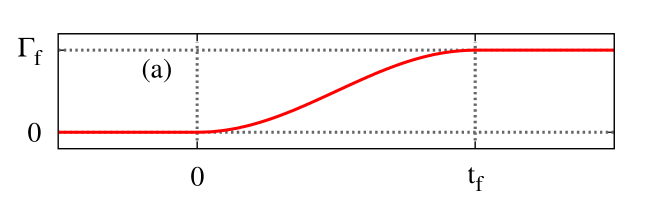
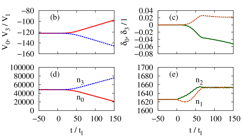
Figure 4: (Color online) (a) Adiabatic ramp of the current from $\Gamma=0$ to a target value of $\Gamma_{\text{f}}$ as a function of the time $t$. Time dependences of (b) the potential depths $V_{0}$ (solid) and $V_{3}$ (dashed) and (c) the displacements of the outer wells $\delta_{0}$ (solid) and $\delta_{3}$ (dashed). (d) and (e) Number of particles in each well.

We calculated the adiabatic current ramp for a condensate of $N=10^{5}$ atoms of ^87Rb with a scattering length tuned to $a=10.9a_{\text{B}}$ ($a_{\text{B}}$ being the Bohr radius). The distance between the middle wells is $l=$2\text{\,}\mathrm{\SIUnitSymbolMicro m}$$. We express the distance of the outer wells by their deviation from a equidistant lattice, i. e. $q_{z}^{0}=-3l/2+\delta^{0}$ and $q_{z}^{3}=3l/2+\delta^{3}$. The basic unit of energy is $E_{l}=\hbar^{2}/ml^{2}$, which yields $E_{l}/h=$29.1\text{\,}\mathrm{Hz}$$. As initial condition we use the ground state for $V_{1}=V_{2}=-80E_{l}$ and $V_{0}=V_{3}=-122E_{l}$. The parameter $d$ in Eq. (11) is chosen such that $\delta^{0}=\delta^{3}=0$ for $t\leq 0$. We have chosen the widths of the trap (1) to be $w_{x}=w_{y}=4l$ and $w_{z}=l/2$. The basic unit of time is $t_{l}=\hbar/E_{l}=$5.47\text{\,}\mathrm{ms}$$. Fig. 4 shows the results for $\Gamma_{f}/J_{12}=0.5$ and $t_{f}/t_{l}\approx 70$.

The trap depth $V_{0}^{0}$ has to be increased, whereas $V_{0}^{3}$ has to be decreased, in an almost symmetric way. The distance of the outer wells has to be varied within a few percent of the distance $l$. The results of the particle numbers in each well confirm that the change of $\Gamma$ is approximately adiabatic (see Fig. 4). For these conditions, the system arrives at an approximate $\mathcal{PT}$-symmetric ground state for $t\gtrsim 70t_{l}$, which can be determined by the constant number of particles in wells $1$ and $2$. We note that the change of the distances of the outer wells can be neglected, as further calculations show. Furthermore, the simulation indicates that the system is robust with respect to small random perturbations of the external potential.

To summarize we have shown that the two middle wells of the Hermitian four-mode model can show the same behavior as the $\mathcal{PT}$-symmetric two-mode model, and thus offers an approach to realize $\mathcal{PT}$ symmetry in a quantum mechanical system. This agreement is exact in the absence of interaction. We have proposed the method of adiabatically increasing the $\mathcal{PT}$ parameter $\Gamma$ to create the $\mathcal{PT}$-symmetric ground state. This works also approximately for particles with interaction in the mean-field limit. We finally estimated parameters of a realistic potential, which would be necessary to prepare such an experiment. The time-dependent potential (1) could be realized e. g. using an acousto-optical modulator Henderson09 . For future work it is desirable to extend these investigations to a BEC described by the full GPE to obtain more accurate parameters for an experimental realization.

- (1) C. M. Bender and S. Boettcher, Phys. Rev. Lett. 80, 5243 (1998)
- (2) S. Klaiman, U. Günther, and N. Moiseyev, Phys. Rev. Lett. 101, 080402 (2008)
- (3) A. Guo, G. J. Salamo, D. Duchesne, R. Morandotti, M. Volatier-Ravat, V. Aimez, G. A. Siviloglou, and D. N. Christodoulides, Phys. Rev. Lett. 103, 093902 (2009)
- (4) C. E. Rüter, K. G. Makris, R. El-Ganainy, D. N. Christodoulides, M. Segev, and D. Kip, Nat. Phys. 6, 192 (2010)
- (5) Y. D. Chong, L. Ge, and A. D. Stone, Phys. Rev. Lett. 106, 093902 (2011)
- (6) L. Ge, Y. D. Chong, S. Rotter, H. E. Türeci, and A. D. Stone, Phys. Rev. A 84, 023820 (2011)
- (7) M. Liertzer, L. Ge, A. Cerjan, A. D. Stone, H. E. Türeci, and S. Rotter, Phys. Rev. Lett. 108, 173901 (2012)
- (8) J. Schindler, A. Li, M. C. Zheng, F. M. Ellis, and T. Kottos, Phys. Rev. A 84, 040101 (2011)
- (9) H. Ramezani, J. Schindler, F. M. Ellis, U. Günther, and T. Kottos, Phys. Rev. A 85, 062122 (2012)
- (10) J. Schindler, Z. Lin, J. M. Lee, H. Ramezani, F. M. Ellis, and T. Kottos, J. Phys. A 45, 444029 (2012)
- (11) S. Bittner, B. Dietz, U. Günther, H. L. Harney, M. Miski-Oglu, A. Richter, and F. Schäfer, Phys. Rev. Lett. 108, 024101 (2012)
- (12) C. M. Bender, V. Branchina, and E. Messina, Phys. Rev. D 85, 085001 (2012)
- (13) E. M. Graefe, U. Günther, H. J. Korsch, and A. E. Niederle, J. Phys. A 41, 255206 (2008)
- (14) E. M. Graefe, H. J. Korsch, and A. E. Niederle, Phys. Rev. Lett. 101, 150408 (2008)
- (15) E.-M. Graefe, H. J. Korsch, and A. E. Niederle, Phys. Rev. A 82, 013629 (2010)
- (16) H. Cartarius and G. Wunner, Phys. Rev. A 86, 013612 (2012)
- (17) H. Cartarius, D. Haag, D. Dast, and G. Wunner, J. Phys. A 45, 444008 (2012)
- (18) Y. Shin, G. B. Jo, M. Saba, T. A. Pasquini, W. Ketterle, and D. E. Pritchard, Phys. Rev. Lett. 95, 170402 (2005)
- (19) R. Gati, M. Albiez, J. Fölling, B. Hemmerling, and M. K. Oberthaler, Applied Physics B 82, 207 (2006), ISSN 0946-2171
- (20) E.-M. Graefe, J. Phys. A 45, 444015 (2012)
- (21) P.-O. Löwdin, J. Chem. Phys. 18, 365 (1950)
- (22) K. Henderson, C. Ryu, C. MacCormick, and M. G. Boshier, New J. Phys. 11, 043030 (2009)