Asymptotics for the Late Arrivals Problem

Abstract

We study a discrete time queueing system where deterministic arrivals have i.i.d. exponential delays $\xi_{i}$. The standard deviation $\sigma$ of the delay is finite, but much larger than the deterministic unit interarrival time. We describe the model as a bivariate Markov chain, we prove that it is ergodic and then we focus on the unique joint equilibrium distribution. We write a functional equation for the bivariate generating function, finding the solution of such equation on a subset of its set of definition. This solution allows us to prove that the equilibrium distribution of the Markov chain decays super-exponentially fast in the quarter plane. Finally, exploiting the latter result, we discuss the numerical computation of the stationary distribution, showing the effectiveness of a simple approximation scheme in a wide region of the parameters. The model, motivated by air and railway traffic, was proposed many decades ago by Kendall [46] with the name of “late arrivals problem”, but no complete solution has been found so far.

1 Introduction

In this paper we consider a single-server queue with deterministic service time, which is assumed of unitary length for the sake of simplicity. The $i$th customer arrives to the system at time

$$t_{i}=i+\xi_{i}\,,\qquad i\in\mathbb{N}\,,$$ (1.1)

where $\{\xi_{i}\}$ are i.i.d. exponential random variables with parameter $\beta$.

In the limit $\beta\to 0$ the point process (1.1) weakly converges to a Poisson process of parameter $1$, whereas for fixed $\beta$ the arrivals are negatively autocorrelated, see [21, 38] and references therein.

Remark 1.

Although the results in [38] are stated under the hypothesis that the probability density function of the delays $\{\xi_{i}\}$ has compact support, this assumption does not play any role in establishing the convergence to a Poisson process. As a consequence, the very same result applies here too.

We study the system described above for fixed $\beta$ and we assume that arriving customers might balk with independent probability $1-\rho$. In other words, each customer can be deleted independently with probability $1-\rho$ before joining the queue. Besides being a mathematical expedient that ensures the existence of a stationary state, the balking is mainly a way to model empty intervals in a constant stream of customers. Again, the point process (1.1) with balking weakly converges to a Poisson process, but with parameter $\rho$ [38]. In what follows, we refer to the balked version of (1.1) as Exponentially Delayed Arrivals (EDA).

Service can be delivered by the unique server only at discrete times. The length of the queue at time $t$ is $n_{t}$; it represents the number of customers waiting to be served, including the customer that will be served precisely at time $t$, if any. Due to the balking, it is immediate to see that the traffic intensity of the system is given by $\rho$; see [38] for details. Using Kendall’s notation we hereafter refer to the queue model described so far as $EDA/D/1$.

The $EDA/D/1$ model is motivated by the description of public and private transportation systems, including buses, trains, aircraft [11, 38, 39, 42] and vessels [35, 43], appointment scheduling in outpatient services [10, 18, 53, 54] crane handling in dock operations [23, 28], and in general any system where scheduled arrivals are intrinsically subject to random variations. Preliminary results show that the model described above fits very well with actual data of inbound air traffic over a large hub, see [17, 50].

The appearance of the stochastic point process (1.1) can be traced back to Winsten’s seminal paper [66]. Winsten named such a queueing model late process and obtained results for the special case $\xi_{i}\in[0,2]$ and service time exponentially distributed. At the end of [66] there is a discussion on Winsten’s results by Lindley, Wishart, Foster, and Takács, where they state that Winsten’s paper can be considered as the first treatment of a queueing model with correlated arrivals [66, pages 22-28].

The same problem was investigated also by Kendall. In [46, page 11] he remarked the great importance of systems with arrivals like (1.1): “[…] perhaps too much attention has been paid to rather uninteresting variations on the fundamental Poisson stream. As soon as one considers variations dictated by the exigencies of the real world, rather than by the pursuit of mathematical elegance, severe difficulties are encountered; this is particularly well illustrated by the notoriously difficult problem of late arrivals.” Kendall also provided the following elegant interpretation: if the random variables $\xi_{i}$ are non-negative then the process defined by (1.1) is the output of the stationary $D/G/\infty$ queueing system [46]. In particular, if the random variables $\xi_{i}$ are exponentially distributed then $EDA/D/1$ can be viewed as a 2-stage tandem queueing network

$$D/M/\infty\rightarrow\cdot/D/1\,.$$

However, this is not the approach followed in this work.

Some years later, under the hypothesis that $\xi_{i}>0$, Nelsen and Williams exactly characterised in [56] the distribution of the inter-arrival time intervals and their correlations. They also gave an explicit expression of these quantities in the particular case of $\xi_{i}$’s exponentially distributed.

After the ’70s only approximations of the arrival process (1.1) [15, 64] or numerical studies of its output [5, 11, 60] seem to have appeared in the literature. In particular, in [38] the authors presented a self-contained study of an arrival process like (1.1), assuming for $\xi_{i}$ a compact-support distribution. They also proposed an approximation scheme that keeps the correlation of the arrivals and is able to compute in a quite accurate way the quantitative features of the queue. To the best of our knowledge, a queueing system with arrivals described by (1.1) still remains an open problem and the best results obtained so far are due to Winstein in 1959 [66].

$EDA/D/1$ is an example of a queueing system with correlated arrivals, a subject broadly studied in past years. There are many ways to impose a correlation to the arrival process. For instance, the parameters of the process may depend on their past realisation, as in [24], or on some on/off sources, as in [67]. Another relevant example of a queue model with correlated arrivals is the so-called Markov Modulated Queueing System. In Markov Modulated Queueing Systems the parameters are driven by an independent external Markovian process, see [2, 9, 22, 52, 61] and references therein. Our model shares with Markov Modulated Queueing Systems the property that one can define an external and independent Markovian process that drives the arrival rates. However, we see in Section 2 that the output of this external drive has also a deterministic effect on the queue length. More precisely, $EDA$ can be interpreted as an independent drawing from an external pool of customers late at time $t$, see (2.2) below. Due to the memoryless property of the exponential delays, each customer late at time $t$ will be still in the pool at time $t+1$ independently with probability $q\equiv e^{-\beta}$. This leads to binomial transitions in the number of late customers.

In Section 2 we show that $EDA/D/1$ can be described as a bivariate Markov chain representing the queue length and the number of late customers. We prove that such a bivariate chain is ergodic and write the balance equations of the stationary distribution, finding a functional equation for the bivariate generating function.

There exists an extensive literature about two-dimensional Markov models. Many methods for attacking the problem are available under two assumptions, namely, spatial homogeneity and finiteness of at least one marginal chain, see [12, 31, 36, 51, 55, 57, 59]. Unfortunately, the Markov chain defined in Section 2 does not satisfy any of the mentioned requirements.

When both components of the Markov chain are infinite but space homogeneity is still ensured, the problem is typically attacked by reduction to a Riemann-Hilbert Boundary Value Problem. These may be solved, for example, by the uniformisation technique [47], conformal mappings [19, 20, 29], the compensation method [3], or the Power Series Approximation [13, 14, 48, 41]. The aforesaid binomial transitions are responsible for the lack of spatial homogeneity and are often encountered in Mathematical Biology [8, 16, 25].

To the best of our knowledge, the functional equation (2.15) below has never previously appeared in the literature. Yet it is possible to mark some analogies with the functional equation in [26, 27, 45], the most important being that in both equations the right hand side exhibits the generating function computed in a convex combination in the parameter $q=e^{-\beta}$. Other examples of chains with binomial transitions may be found in [1, 6, 58, 69].

In Section 3 we study the marginal distribution of the number of late customers and we obtain its exact analytical expression, which reveals the rich combinatorial structure of the problem. This intermediate result allows us to show that the stationary distribution of the $EDA/D/1$ queue has a super-exponential decay. Finally, in Section 4 we show that such a super-exponential behaviour enables a simple, yet very effective, numerical approximation scheme of the system balance equations. For a wide range of the system parameters, including typical values for real traffic applications of the model, we give a very good a priori estimate of the total-variation distance between the true and the approximate solution.

2 Stationary distribution: generating function and balance equations

Let us consider the process $n_{t}$, which describes the length of the queue at time $t$. This process is governed by the stochastic recursion

$$n_{t+1}=n_{t}+m_{(t,t+1]}-(1-\delta_{n_{t},0})\,,$$ (2.1)

where $m_{(t,t+1]}$ is the number of arrivals in the interval $(t,t+1]$ according to the arrival process (1.1), and $\delta_{i,j}$ is the usual Kronecker’s delta. The term $1-\delta_{n_{t},0}$ represents the action of the server in decreasing the queue length by one if at time $t$ the queue is non-empty. Since the service time is deterministic, we focus on the so-called embedded process by observing the system at $t\in\mathbb{N}$, i. e. at departure instants.

The quantity $m_{t}\equiv m_{(t,t+1]}$ depends in general on the whole previous history of the system. Indeed, if for some large value of $T$, $m_{s}=0$ for any $s\in\{t-T,t-T+1,...,t-1\}$ then $m_{t}$ is large with great probability. Conversely, if in the recent past the values of $m_{s}$ have been large then $m_{t}$ is expected to be small. This suggests that the arrival process is negatively autocorrelated, as proven in [38]. Hence, the recursion (2.1) does not depend only on the present value of $n_{t}$, and the memory of the process is infinite since $T$ can be arbitrarily large.

Let us now denote by $l_{t}$ the number of customers that are late at time $t$, that is to say,

$$l_{t}\equiv\big{|}\{0\leq i\leq t\text{ such that }\xi_{i}>t-i\}\big{|}\,.$$ (2.2)

Let us next define $p\equiv\int_{0}^{1}f_{\xi}(t)dt=\int_{0}^{1}\beta e^{-\beta t}dt=1-e^{-\beta}$ and $q\equiv e^{-\beta}$. Given the value of $l_{t}$, the random variable $m_{t}$ is binomial with parameters $l_{t}$ and $p$. According to the memoryless property of the exponential delays $\{\xi_{i}\}$, the number of unit time intervals in which a customer is late is a geometric random variable with parameter $q$. In other words, a customer will be late for $k$ consecutive time intervals with probability $q^{k}p$. Hence, the embedded process $l_{t}$, $t\in\mathbb{N}$, is a discrete-time Markov chain. If the customer scheduled in the interval $(t,t+1]$ has balked then

$$P\left(m_{t}=j\,|\,l_{t}=l\right)=\binom{l}{j}p^{j}q^{l-j}\equiv b_{j,l}\,,$$ (2.3)

otherwise

$$P\left(m_{t}=j\,|\,l_{t}=l\right)=\binom{l+1}{j}p^{j}q^{l+1-j}=b_{j,l+1}\,.$$

All in all,

$$P\left(m_{t}=j\,|\,l_{t}=l\right)=b_{j,l}\,(1-\rho)+b_{j,l+1}\,\rho\,.$$ (2.4)

We describe the $EDA/D/1$ queue by the embedded process $(n_{t},l_{t})$, $t\in\mathbb{N}$, a discrete-time Markov chain with the following transition probabilities:

$$\text{For }n>0,$$ (2.5)

$$\quad\mathcal{P}\left((n,l),(n+a-1,l-a+1)\right)=\rho\,b_{a,l+1}\,, 0\leq a\leq l\!+\!1\,,$$

$$\quad\mathcal{P}\left((n,l),(n+a-1,l-a)\right)=(1-\rho)\,b_{a,l}\,, 0\leq a\leq l\,;$$

$$\text{For }n=0,$$ (2.6)

$$\quad\mathcal{P}\left((0,l),(a,l-a+1)\right)=\rho\,b_{a,l+1}\,, 0\leq a\leq l\!+\!1\,,$$

$$\quad\mathcal{P}\left((0,l),(a,l-a)\right)=(1-\rho)\,b_{a,l}\,, 0\leq a\leq l\,.$$

Figure 1 displays the transitions of the embedded chain $(n_{t},l_{t})$ in the quarter plane.

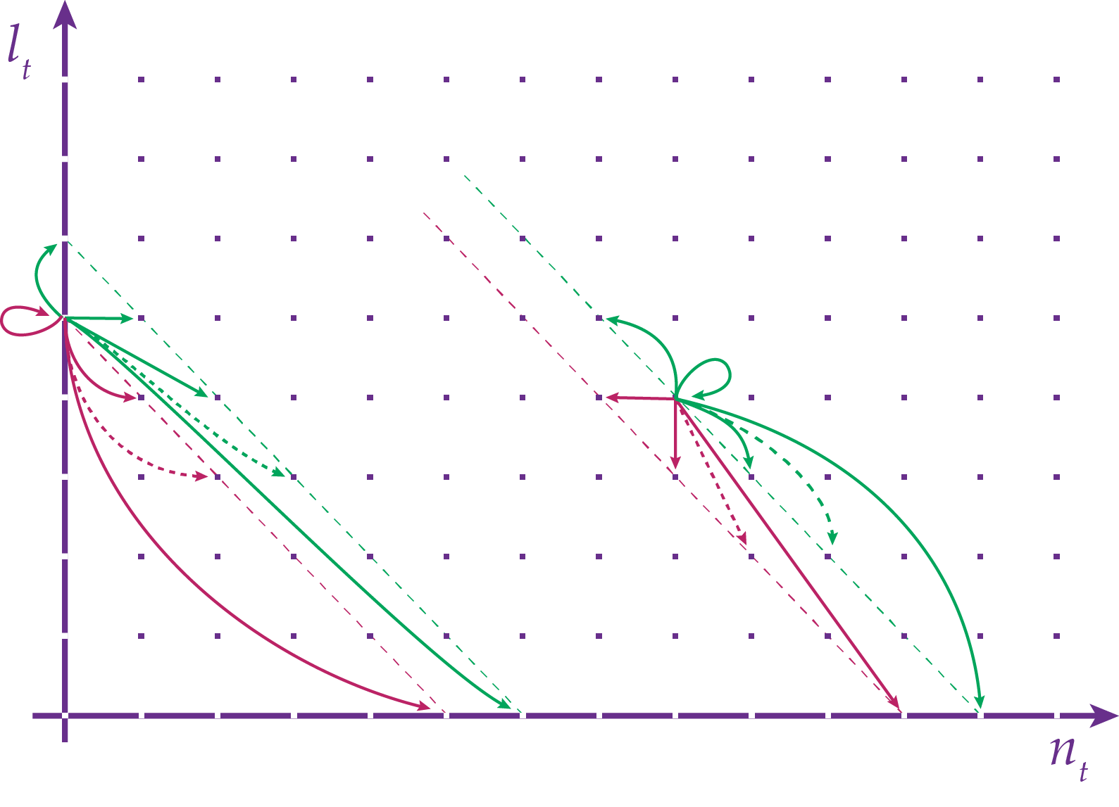
Figure 1: Transitions of the $EDA/D/1$ queueing system in the quarter plane. They happen along the lines of Cartesian equation $x+y=n_{t}+l_{t}$ and $x+y=n_{t}+l_{t}-1$ if $n_{t}\neq 0$, and along the lines of Cartesian equation $x+y=n_{t}+l_{t}$ and $x+y=n_{t}+l_{t}+1$ if $n_{t}=0$. Green transitions happen with probability $\rho$ (no balking), red transitions happen with probability $1-\rho$ (balking).

We now address the existence of the stationary state of the embedded chains $l_{t}$ and $(n_{t},l_{t})$.

Lemma 1 The chain $l_{t}$ is ergodic if and only if $q<1$.

Proof.

If $q<1$, the chain $l_{t}$ is clearly irreducible. In order to prove its positive recurrence, we use Foster’s criterion [63, Cor. 8.7] setting $f(l_{t})=l_{t}+1$ as the Lyapunov function. Thus, we need to show that there exist suitable positive constants $K,\gamma$ such that

1. $\mathbb{E}\left[f(l_{1})-f(l_{0})\,|\,l_{0}=L\right]\leq-\gamma$ for $f(L)>K$;

2. $\mathbb{E}\left[f(l_{1})\,|\,l_{0}=L\right]<\infty$ for $f(L)\leq K$;

3. the set $\{l\geq 0\,:\,f(l)\leq K\}$ is finite.

First, by (2.4),

$$\mathbb{E}\left[f(l_{1})-f(l_{0})\,|\,l_{0}=L\right] =Lq(1-\rho)+(L+1)q\rho-L\,,$$

$$=\rho q-L(1-q)\,.$$ (2.7)

Therefore, point 1 is satisfied, for instance, by the choice $\gamma=1$ and $K=1+\frac{1+\rho q}{1-q}$. Next, Figure 1 shows that at each iteration $l_{t}$ increases at most by one unit and point 2 is satisfied:

$$\mathbb{E}\left[f(l_{1})\,|\,l_{0}=L\right]\leq L+2\,.$$ (2.8)

By definition of $f(l_{t})$ point 3 is also fulfilled. On the other hand, for $q=1$ the chain $l_{t}$ is not ergodic because it is no longer irreducible. ∎

Lemma 2 The bivariate chain $(n_{t},l_{t})$ is ergodic if and only if $q<1$ and $\rho<1$.

Proof.

If $q<1$ and $\rho<1$, the bivariate chain $(n_{t},l_{t})$ is irreducible, see Figure 1. Let us consider the process $\alpha_{t}=n_{t}+l_{t}$, which represent the diagonal in the quarter plane where the point $(n_{t},l_{t})$ lies on, see Figure 1. The bivariate chain has the property that $|\alpha_{t+1}-\alpha_{t}|\leq 1$. Equations (2.5)-(2.6) yield

$$P(\alpha_{t+1}=\alpha_{t}+1\,|\,n_{t}\neq 0)=0\,,$$ (2.9)

$$P(\alpha_{t+1}=\alpha_{t}-1\,|\,n_{t}\neq 0)=(1-\rho)\,,$$ (2.10)

$$P(\alpha_{t+1}=\alpha_{t}+1\,|\,n_{t}=0)=\rho\,,$$ (2.11)

$$P(\alpha_{t+1}=\alpha_{t}-1\,|\,n_{t}=0)=0\,.$$ (2.12)

In order to prove the positive recurrence of $(n_{t},l_{t})$, we use again Foster’s criterion setting $f(n_{t},l_{t})=M\alpha_{t}+l_{t}+1$ with $M=\nicefrac{{2}}{{(1-\rho)}}$. From (2.7) and (2.9)-(2.12),

$$\mathbb{E}\left[f(n_{1},l_{1})-f(n_{0},l_{0})\,|\,n_{0}=N,l_{0}=L\right]$$

$$\qquad=M\mathbb{E}\left[\alpha_{1}-\alpha_{0}\,|\,n_{0}=N,l_{0}=L\right]+\mathbb{E}\left[l_{1}-l_{0}\,|\,l_{0}=L\right]\,,$$

$$\qquad\leq M\rho\delta_{N,0}-M(1-\rho)(1-\delta_{N,0})+\rho q-L(1-q)\,.$$

Then, using a little algebra, it can be shown that the first point of Foster’s criterion is satisfied by $\gamma=1$ and $K>1+\frac{(M+1)(1+\rho q+M\rho)}{1-\rho}$ (for example, $K=\frac{7}{(1-\rho)^{2}(1-q)}$). Point 2 of Foster’s criterion holds because

$$\mathbb{E}\left[f(n_{1},l_{1})\,|\,n_{0}=N,l_{0}=L\right]\leq M(N+L+1)+L+2,$$

where we have used the property that $\alpha_{t}$ has only nearest-neighbour transitions and equation (2.8). Point 3 is fulfilled by simply considering the definition of $f(n_{t},l_{t})$. For $\rho=1$, the bivariate chain $(n_{t},l_{t})$ is not ergodic because it is no longer irreducible. ∎

For $\rho,q<1$, Lemma 2 guarantees both the existence and the uniqueness of the stationary distribution

$$P_{n,l}\equiv\lim_{t\to\infty}P(n_{t}=n,l_{t}=l)\,.$$ (2.13)

Let us consider the following bivariate generating function:

$$P(z,y)=\sum_{n,l\geq 0}\,z^{n}\,y^{l}\,P_{n,l}\,,\quad|z|,|y|\leq 1\,.$$ (2.14)

We are now ready to prove the main result of this section.

Theorem 1.

The bivariate generating function (2.14) satisfies

$$P(z,y) =\frac{1+\rho\,(\upsilon-1)}{z}\left[(z-1)\,P(0,\upsilon)+P(z,\upsilon)\right]\,,$$ (2.15)

where $\upsilon=\upsilon(z,y)=z+q\,(y-z)$.

Remark 2.

The functional equation (2.15) does not admit simple or immediate solutions. It is radically different from the functional equations typically studied in the literature [20, 30] and it is rather special in this respect. A simple solution can be found only in the particular case $z=1$, see Section 3 below.

Proof 2.1 (Proof of Theorem 1).

For each $n,l\geq 0$, the balance equations of $EDA/D/1$ are the following:

$$P_{n,l}=(1-\rho)\left(\sum_{j=0}^{n}P_{j+1,l+n-j}\,b_{n-j,l+n-j}+P_{0,l+n}\,b_{n,l+n}\right)\\ +\rho\left(\sum_{j=0}^{n}\!P_{j+1,l+n-j-1}\,b_{n-j,l+n-j}+P_{0,l+n-1}\,b_{n,l+n}\right),$$ (2.16)

where $b_{j,l}$ are given by (2.3) and we agree that $P_{n,l}=0$ whenever $n,l<0$. The special cases $n=0$ and $n=l=0$ respectively lead to

$$P_{0,l}=(1-\rho)\left(P_{1,l}+P_{0,l}\right)\,b_{0,l}+\rho\left(P_{1,l-1}+P_{0,l-1}\right)\,b_{0,l}\,,$$ (2.17)

$$P_{0,0}=(1-\rho)(P_{1,0}+P_{0,0})\,.$$ (2.18)

To show that (2.16)–(2.18) hold, it suffices to write $P_{n_{t+1},l_{t+1}}$ in terms of $P_{n_{t},l_{t}}$ and then neglect the time dependency. Take for example (2.18): the system is found at time $t+1$ in state $(0,0)$, i. e. with empty queue and no late customers, only if at time $t$ it was either in state $(0,0)$ or in state $(1,0)$, and the $(t+1)$th scheduled customer is deleted by thinning. Indeed, if at time $t$ the system was in state $(0,0)$ then nothing happens and the state remains unchanged, whereas if it was in state $(1,0)$ then the customer in queue is served and at time $t+1$ the system is in state $(0,0)$. Similarly, there are four cases such that the system is found at time $t+1$ in state $(0,l)$, i. e. with an empty queue and $l$ customers late. In the first two cases the system is in state $(1,l)$ or in state $(0,l)$ at time $t$, the $(t+1)$th customer is deleted, and no one of the $l$ late customers arrives in the interval $[t,t+1)$ (this event has in fact probability $q^{l}=b_{0,l}$). In the remaining cases the system is in state $(1,l-1)$ or in state $(0,l-1)$ at time $t$, the $(t+1)$th customer is not deleted, and no one of the $(l-1)+1$ late customers arrive in the interval $(t,t+1]$. The latter argument gives (2.17) while an easy generalisation to the case $n\geq 1$ leads to (2.16).

Let us take (2.16), multiply both sides by $z^{n}\,y^{l}$, and then sum over $n$ and $l$. The summation of all terms multiplied by $(1-\rho)$ yields

$$(1-\rho)\Bigg{\{}\sum_{n,l\geq 0}\Bigg{[}\sum_{j=0}^{n}P_{j+1,l+n-j}{n+l-j\choose n-j}z^{j}(zp)^{n-j}(yq)^{l}\\ +P_{0,l+n}{l+n\choose n}(zp)^{n}(yq)^{l}\Bigg{]}\Bigg{\}}\,,$$

or equivalently,

$$(1-\rho)\Bigg{\{}\sum_{j\geq 0}\sum_{n\geq j}\Bigg{[}\sum_{l\geq 0}P_{j+1,l+n-j}{n+l-j\choose n-j}z^{j}(zp)^{n-j}(yq)^{l}\\ +P_{0,l+n}{l+n\choose n}(zp)^{n}(yq)^{l}\Bigg{]}\Bigg{\}}\,.$$

The change of indices $k=n-j$ and $m=l+n-j=l+k$ yields

$$(1-\rho)\Bigg{\{}\sum_{j\geq 0}\sum_{n\geq j}\Bigg{[}\sum_{l\geq 0}P_{j+1,l+n-j}{n+l-j\choose n-j}z^{j}(zp)^{n-j}(yq)^{l}\Bigg{\}}$$

$$=(1-\rho)\Bigg{\{}\sum_{j\geq 0}z^{j}\sum_{m\geq 0}\Bigg{[}\sum_{k=0}^{n}P_{j+1,m}{m\choose k}(zp)^{k}(yq)^{m}\Bigg{]}\Bigg{\}}\,,$$

$$=\frac{1-\rho}{z}\sum_{j\geq 1}\sum_{m\geq 0}P_{j,m}z^{j}(zp+yq)^{m},$$

$$=\frac{1-\rho}{z}\left[P(z,zp+yq)-P(0,zp+yq)\right]\,,$$

to which we still have to sum the contribution

$$(1-\rho)\sum_{n,l\geq 0}P_{0,l+n}{l+n\choose n}(zp)^{n}(yq)^{l}=(1-\rho)P(0,zp+yq)\,.$$

All in all, the sum of all terms multiplied by $(1-\rho)$ is

$$(1-\rho)\left[P(0,zp+yq)+\frac{1}{z}\left(P(z,zp+yq)-P(0,zp+yq)\right)\right].$$

In a completely analogous way we can compute the sum of the terms multiplied by $\rho$, which turns out to be

$$\rho(zp+yq)\Big{[}P(0,zp+yq)+\frac{1}{z}\left(P(z,zp+yq)-P(0,zp+yq)\right)\Big{]}.$$

Summing up the two contributions, we get (2.15).

Remark 3.

We end this section with a discussion of the special case $q=0$. In this regime, the right-hand side of equation (2.15) does not depend on $y$ anymore, and $P(z,y)\equiv Q(z)$. The number of late customers is in fact $l_{t}=0$ as the $i$th customer can not have a delay $\xi_{i}\geq 1$. Then, equation (2.15) yields directly

$$Q(z)=\frac{1+\rho(z-1)}{z}[(z-1)Q(0)+Q(z)]\,,$$ (2.19)

where $Q(0)=1-\rho$ is the stationary probability of a void queue. Therefore, equation (2.19) is equivalent to

$$Q(z)=1+\rho(z-1)\,,$$

which is the classical result of a $D/D/1$ queue with balking.

3 The marginal distribution of late customers

In this section we focus on $P_{l}$, the marginal distribution of late customers. First, we iterate the functional equation (2.15) to obtain the generating function of $P_{l}$ in the form of an infinite product. Then, we invert the generating function and find the exact analytical expression of $P_{l}$. Finally, we derive the asymptotic behaviour of $P_{l}$ and use it to infer asymptotics for $P_{n,l}$.

The marginal distribution of late customers is

$$P_{l}=\sum_{n\geq 0}P_{n,l}$$

and its generating function is

$$\sum_{l\geq 0}P_{l}y^{l}=\sum_{n,l\geq 0}P_{n,l}\,y^{l}=P(1,y)\,.$$

Setting $z=1$ into equation (2.15) yields

$$P(1,y)=[1+\rho q(y-1)]P(1,1+q(y-1))\,.$$ (3.1)

Evaluating the last equation in $(1,1+q(y-1))$ yields

$$P(1,1+q(y-1))=[1+\rho q^{2}(y-1)]P(1,1+q^{2}(y-1))\,.$$

Iterating (3.1) $N$ times,

$$P(1,y)=\left[\prod_{k=0}^{N-1}1+\rho q^{k+1}(y-1)\right]P(1,1+q^{N}(y-1))\,.$$

The limit of $\prod_{k=0}^{N-1}[1+\rho q^{k+1}(y-1)]$ for $N\to\infty$ exists for each $q<1$ and $y\in\mathbb{C}$, see [4]. Moreover, $\lim_{N\to\infty}P(1,1+q^{N}(y-1))=1$ Therefore, we have proven the following

Corollary 3 For $q<1$ and $|y|\leq 1$,

$$P(1,y)=\prod_{k\geq 0}\left[1+\rho q^{k+1}(y-1)\right]\,.$$ (3.2)

Remark 4.

The infinite product (3.2) has an interesting combinatorial interpretation:

$$P(1,y)=\prod_{k\geq 0}\left[1+\rho q^{k+1}(y-1)\right]=\frac{(\rho(1-y);q)_{\infty}}{1+\rho(y-1)}\,,$$ (3.3)

where $(a;q)_{\infty}=\prod_{k\geq 0}[1-aq^{k}]$ is the infinite $q$-Pochhammer symbol, also known as infinite $q$-ascending factorial in $a$. For $y=1-\nicefrac{{q}}{{\rho}}$, $P(1,y)=\phi(q)\,(1-q)^{-1}$, where $\phi(q)$ is the well-known Euler function.

Remark 5.

For $q<1$, the right-hand side of (3.3) is analytic for each $y\in\mathbb{C}$. Therefore, the power series $P(1,y)=\sum_{l\geq 0}P_{l}\,y^{l}$, convergent for each $|y|\leq 1$, can be analytically continued in the whole complex plane. As such, we expect the marginal distribution $P_{l}$ to decrease super-exponentially fast in $l$.

Following the insight given by Remark 5, we shift now the focus to the asymptotic behaviour of $P_{l}$ and $P_{n,l}$. Expanding the product and rearranging it in powers of $\rho(y-1)$ yields

$$P(1,y) =\prod_{k\geq 0}\left(1+\rho\,q^{k+1}(y-1)\right)$$

$$=1+\sum_{k\geq 1}\rho^{k}(y-1)^{k}\left[\sum_{m\geq{k+1\choose 2}}d(m;k)q^{m}\right],$$ (3.4)

where $d(m;k)$ is the number of partitions of $m$ in $k$ distinct parts.

The following theorem holds:

Theorem 2.

Let $P_{l}$ be the equilibrium marginal distribution of the number of late customers and $P(1,y)$ its generating function. Then,

$$P(1,y) =\sum_{k\geq 0}\frac{\rho^{k}q^{{k+1\choose 2}}(y-1)^{k}}{\prod_{i=1}^{k}[1-q^{i}]}\,,$$ (3.5)

$$P_{l} =\sum_{k\geq l}\frac{(-1)^{k-l}\rho^{k}q^{{k+1\choose 2}}{k\choose l}}{\prod_{i=1}^{k}[1-q^{i}]}\,.$$ (3.6)

Theorem 2 is a direct consequence of the following two results from number theory.

Lemma 4 [68] If $m>\binom{k+1}{2}$ then the number of partitions of $m$ in $k$ distinct parts equals the number of partitions of $m-\binom{k+1}{2}$ into at most $k$ parts (not necessarily distinct).

Lemma 5 [7, 40] Let $p_{\leq k}(m)$ be the number of partitions of $m$ in parts that do not exceed $k$. Then $p_{\leq k}(m)$ equals the number of partitions of $m$ into at most $k$ parts and

$$P_{\leq k}(q)=\sum_{m\geq 0}p_{\leq k}(m)\,q^{m}=\prod_{i=1}^{k}\frac{1}{1-q^{i}}\,.$$

Proof 3.1 (Proof of Theorem 2).

Using Lemma 3 and 3 we can recast (3.4) as

$$P(1,y) =1+\sum_{k\geq 1}\rho^{k}(y-1)^{k}\left[\sum_{m\geq{k+1\choose 2}}d(m;k)q^{m}\right],$$

$$=1+\sum_{k\geq 1}\rho^{k}(y-1)^{k}q^{{k+1\choose 2}}\left[1+\sum_{m>0}d\left(m+{k+1\choose 2};k\right)q^{m}\right],$$

$$=1+\sum_{k\geq 1}\rho^{k}(y-1)^{k}q^{{k+1\choose 2}}\left[1+\sum_{m>0}p_{\leq k}(m)q^{m}\right],$$

$$=1+\sum_{k\geq 1}\rho^{k}(y-1)^{k}q^{{k+1\choose 2}}\prod_{i=1}^{k}\frac{1}{1-q^{i}}\,,$$

$$=\sum_{k\geq 0}\frac{\rho^{k}q^{{k+1\choose 2}}(y-1)^{k}}{\prod_{i=1}^{k}[1-q^{i}]}\,,$$

where, as usual, $p_{\leq k}(0)=1$ and $\prod_{i=a}^{b}f_{k}=1$ when $b<a$.

The second part of the Theorem is proved from (3.5) as follows:

$$P_{l} =\frac{1}{l!}\frac{d^{l}}{dy^{l}}P(1,y)\Big{|}_{y=0}\,,$$

$$=\sum_{k\geq l}\frac{\rho^{k}q^{{k+1\choose 2}}}{\prod_{i=1}^{k}[1-q^{i}]}\frac{1}{l!}\frac{d^{l}}{dy^{l}}(y-1)^{k}\Big{|}_{y=0}\,,$$

$$=\sum_{k\geq l}\frac{(-1)^{k-l}\rho^{k}q^{{k+1\choose 2}}{k\choose l}}{\prod_{i=1}^{k}[1-q^{i}]}\,.$$

Now we use (3.6) to obtain an upper bound on $P_{l}$: let $(q;q)_{l}=\prod_{i=1}^{l}\left[1-q^{i}\right]$ be the $q$-Pochammer symbol of the pair $(q,q)$. The following inequalities hold:

$${m+l\choose l} =\prod_{k=1}^{m}\left(1+\frac{l}{k}\right)\leq(1+l)^{m}\,,$$

$$\prod_{i=l+1}^{l+m}\left[1-q^{i}\right] \geq\prod_{i=1}^{m}\left[1-q^{i}\right]=(q;q)_{m}\,,$$

$$(q;q)_{l} \geq(q;q)_{\infty}\,.$$

Thus,

$$P_{l} =\frac{\rho^{l}\,q^{{l+1\choose 2}}}{(q;q)_{l}}\sum_{m\geq 0}\frac{(-\rho)^{m}q^{(l+1)m}q^{{m\choose 2}}\,{m+l\choose l}}{\prod_{i=l+1}^{l+m}[1-q^{i}]}\;,$$

$$\leq\frac{\rho^{l}\,q^{{l+1\choose 2}}}{(q;q)_{\infty}}\sum_{m\geq 0}\frac{q^{{m\choose 2}}[\rho\,q^{l+1}\,(l+1)]^{m}}{(q;q)_{m}}\;,$$ (3.7)

$$=\rho^{l}\,q^{{l+1\choose 2}}\frac{\prod_{k\geq 0}\left[1+q^{k+l+1}\rho(l+1)\right]}{(q;q)_{\infty}}\,,$$ (3.8)

where from (3.7) to (3.8) we have used the properties of $q$-ascending factorials and $q$-binomial coefficients [32]. If $l$ is sufficiently large then $q^{l}\rho(l+1)\leq 1$, and (3.8) yields

$$P_{l}\leq\rho^{l}\,q^{{l+1\choose 2}}\frac{(-q;q)_{\infty}}{(q;q)_{\infty}}\,.$$ (3.9)

Remark 6.

Theorem 2 and (3.9) show that, asymptotically in $l$, the leading order of $P_{l}$ is $\rho^{l}q^{{l+1\choose 2}}$. This fact can be directly implied from arrival process (1.1). In fact, the most likely way to have $l$ late customers ($l$ large) is that each of the customers originally scheduled in the interval $[t-l,t)$ do not balk and are late at time $t$, an event of probability $\rho q^{l}\,\rho q^{l-1}\cdots\rho q=\rho^{l}q^{{l+1\choose 2}}$.

Since $P_{n,l}\leq P_{l}$, we have just obtained the following asymptotic result:

Theorem 3.

Uniformly in $n$, the equilibrium distribution $P_{n,l}$ decays super-exponentially fast in $l$. More precisely,

$$P_{n,l}=O\left(\rho^{l}q^{{l+1\choose 2}}\right)\quad\text{for }l\to\infty\,.$$ (3.10)

As a matter of fact the super-exponential decay of $P_{n,l}$ may be proved asymptotically in $n$. Let us consider the auxiliary process $\alpha_{t}=n_{t}+l_{t}$, which we have already encountered in the proof of Lemma 2. There we have interpreted $\alpha_{t}$ as the diagonal in the quarter plane where the point $(n_{t},l_{t})$ lies on. Under equilibrium conditions, the probability of finding the system on the $a$th diagonal is just

$$p_{a}\equiv P(\alpha_{t}=a)=\sum_{\begin{subarray}{c}n,l\geq 0\\ n+l=a\end{subarray}}P_{n,l}\,,\quad a\geq 0\,.$$

It is straightforward to prove that the generating function of $p_{a}$ is $P(z,z)$.

Substituting $y=z$ into (2.15) yields

$$P(z,z)=\frac{1+\rho(z-1)}{1-\rho}P(0,z)\,.$$ (3.11)

Remark 7.

Equation (3.11) gives an interesting connection between the equilibrium distribution of the quantity $\alpha_{t}=n_{t}+l_{t}$ and the stationary probability of having $l$ late customers given that the queue is void. Figure 1 shows that the latter event drives the dynamic of $\alpha_{t}$ through an independent Bernoulli random variable with parameter $\rho$, which explains the factor $1+\rho(z-1)$.

From (3.11) we can compute as follows $p_{a}$ in terms of $P_{0,a}$:

$$p_{a} =\frac{1}{a!}\,\frac{d^{a}}{dz^{a}}P(z,z)\Big{|}_{z=0}$$

$$=\frac{1}{a!}\,\Big{[}\frac{1+\rho(z-1)}{1-\rho}\frac{d^{a}}{dz^{a}}P(0,z)+\frac{\rho\,a}{1-\rho}\frac{d^{a-1}}{dz^{a-1}}P(0,z)\Big{]}_{z=0}\,,$$

$$=P_{0,a}+\frac{\rho}{1-\rho}P_{0,a-1}\,.$$ (3.12)

For $a=n+l$, formulas (3.10) and (3.12) then yield

$$P_{n,l}\leq p_{a}=P_{0,a}+\frac{\rho}{1-\rho}P_{0,a-1}=O(\rho^{a}q^{\binom{a}{2}})\,.$$ (3.13)

Therefore, the following asymptotic result holds:

Theorem 4.

The equilibrium distribution $P_{n,l}$ decays super-exponentially fast as either $n\to\infty$ or $l\to\infty$. More precisely,

$$P_{n,l}=O\left(\rho^{n+l}q^{{n+l\choose 2}}\right)\quad\text{for }n,l\to\infty\,.$$ (3.14)

4 Numerical approximation of the joint stationary measure

In this final section we examine the possibility to approximately compute the joint stationary distribution $P_{n,l}$. Due to the very broad range of applications of the queueing model $EDA/D/1$, an efficient approximate computation of the solution may prove itself crucial in contexts where practical solutions are needed.

In Section 3 we have shown that the joint stationary probability $P_{n,l}$ decreases super-exponentially fast in the limit of either $n,l\to\infty$. The natural question arising is then whether a bare truncation of the infinite linear system (2.16)-(2.18) is sufficient to obtain a satisfactory numerical expression of $P_{n,l}$. As we will see, in this case the answer is positive due to (3.14).

We truncate the infinite system of balance equations (2.16)-(2.18) by fixing an integer $\alpha_{\max}$ and imposing $P_{n,l}=0$ for $n+l>\alpha_{\max}$. For the purpose of simplifying the notation, we map the quarter plane $\{n,l\in\mathbb{N}\times\mathbb{N}\}$ onto the set of non-negative integers. This way, we can relabel the unknowns $P_{n,l}$ as $\pi_{i}$ and recast (2.16)-(2.18) as $\pi=\pi Q$. For the details of both mapping and relabeling, see Appendix A. Next, we map $\{n,l\in\mathbb{N}\times\mathbb{N}\text{ such that }n+l\leq\alpha_{\max}\}$ onto the set of non-negative integers $\{0,1,\ldots,k_{\max}\}$, where $k_{\max}={\alpha_{\max}+1\choose 2}$. We want to consider the truncated system

$$\begin{cases}&\tilde{\pi}_{i}=\sum_{j=0}^{k_{\max}}\tilde{\pi}_{j}Q_{j,i}\qquad i=1,2,\ldots,k_{\max}-1\,,\\ &\sum_{j=0}^{k_{\max}}\tilde{\pi}_{j}=1\,.\end{cases}$$ (4.1)

The idea we present is not new and has been already discussed, for instance in [65] for stationary distributions with geometric tail. As shown in Appendix B, there exists a sequence $\{\varepsilon_{j}\}$ such that

$$\sum_{i>k_{\max}}\pi_{i}\,Q_{i,j}\leq\varepsilon_{j}\,,\qquad j=0,1,\ldots,k_{\max}-1\,,$$

$$\sum_{i>k_{\max}}\pi_{i}\leq\varepsilon_{k_{\max}}\,.$$

The following a priori estimate of the error introduced by the truncation can be obtained from perturbation theory [34, §2.6.2]:

$$\sum_{j=0}^{k_{\max}}|\pi_{j}-\tilde{\pi}_{j}|\leq\kappa(A)\sum_{i=0}^{k}\varepsilon_{i}\,,$$ (4.2)

where $A$ is the $k_{\max}\times k_{\max}$ matrix

$$A_{ij}=\begin{cases}\delta_{i,j}-Q_{i,j}\,,&\quad i=0,1,\ldots,k_{\max}-1\,,\\ 1&\quad i=k_{\max}\,,\end{cases}$$ (4.3)

$\delta_{i,j}$ is the usual Kronecker’s delta, and

$$\kappa(A)=\|A\|_{1}\|A^{-1}\|_{1}$$

is the norm-1 condition number of the matrix $A$.

From Appendix B,

$$\sum_{j=0}^{k_{\text{\tiny max}}}\varepsilon_{j}\leq 2\alpha_{\max}\frac{(-q;q)_{\infty}}{(q;q)_{\infty}}\rho^{\alpha_{\text{\tiny max}}+1}q^{{\alpha_{\text{\tiny max}}+1\choose 2}}\leq 2\alpha_{\max}\frac{(-q;q)_{\infty}}{(q;q)_{\infty}}q^{{\alpha_{\text{\tiny max}}+1\choose 2}}\,.$$ (4.4)

Figure 2 shows the behaviour of $\log\left(\frac{(-q;q)_{\infty}}{(q;q)_{\infty}}q^{{\alpha_{\text{\tiny max}}\choose 2}}\right)$ as a function of $q$ for $\alpha_{\max}=100$. Therefore, unless the condition number of the matrix $A$ is very large, we expect that a truncation at the level $\alpha_{\max}=100$ will give a very good approximation of the stationary probabilities of $EDA/D/1$.

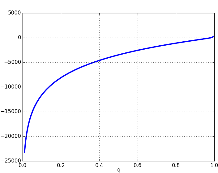
Figure 2: Behaviour of $\log\left(\frac{(-q;q)_{\infty}}{(q;q)_{\infty}}q^{{\alpha_{\text{\tiny max}}\choose 2}}\right)$ as a function of $q$ for $\alpha_{\max}=100$.

Estimating the condition number of a matrix is a notably difficult problem and a vast literature exists on this topic, see e. g. [33, 62, 44]. Since the aim of the present section is showing that a bare truncation of the balance equations (2.5)–(2.6) may be sufficient for an approximate computation of $P_{n,l}$, we fall back on numerical computations. Figure 3 displays the value of $\kappa(A)$ in the $\rho q$-plane when $\alpha_{\max}=100$. We see that the condition number is not larger than $10^{5}$ for $\rho,q\leq 0.99$.

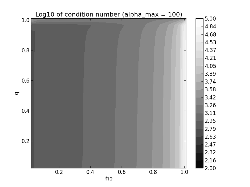
Figure 3: $\log_{10}\kappa(A)$ for $\alpha_{\max}=100$ when $\rho$ and $q$ vary between $0.0$ and $0.99$ in $25$ steps. The condition number is of order $10^{5}$ at most in this region of the parameters.

Table 1 gives the numerical value of the right-hand side of (4.4) for $q$ between $0.9$ and $0.99$, and $\alpha_{\max}=100$. Comparison of Table 1 with Figure 3 shows that, uniformly in $\rho\leq 0.99$, the a priori norm-1 approximation error is less than $10^{-12}$ for $q$ up to $0.98$.

Table 1: Value of $2\alpha_{\max}\frac{(-q;q)_{\infty}}{(q;q)_{\infty}}q^{{\alpha_{\text{\tiny max}}\choose 2}}$ for $0.90\leq q\leq 0.99$ and $\alpha_{\max}=100$.

$0.90$	$0.91$	$0.92$	$0.93$	$0.94$
$1.4\times 10^{-224}$	$9.8\times 10^{-200}$	$5.1\times 10^{-175}$	$2.4\times 10^{-150}$	$1.3\times 10^{-125}$
$0.95$	$0.96$	$0.97$	$0.98$	$0.99$
$1.3\times 10^{-100}$	$5.6\times 10^{-75}$	$8.7\times 10^{-48}$	$2.3\times 10^{-16}$	$2.6\times 10^{33}$

Remark 8.

For air traffic applications, $q=0.98$ corresponds to typical delays of the order of one hour. The same value of $q$ for other transport systems, e. g. trains or buses, correspond to even higher delays. Consider also that typical values of $\rho$ in extremely congested systems, e. g. London Heathrow Airport, do not exceed $0.98$, see [17]. Therefore, the approximation scheme presented in this section is very fit for real life applications.

Finally, Figure 3 suggests that the system condition number is decreasing in $q$ for fixed $\rho$. Figure 4 validates this insight by showing a log-log plot of the condition number for $\alpha_{\max}$ between $10$ and $100$ and $\rho=0.95$. The very same figure also suggests that the condition number of the system may grow polynomially with $\alpha_{\max}$. In particular, $\kappa(A)$ seems to grow linearly in $\alpha_{\max}$ for $\rho=0.95$ and $q=0.0$.

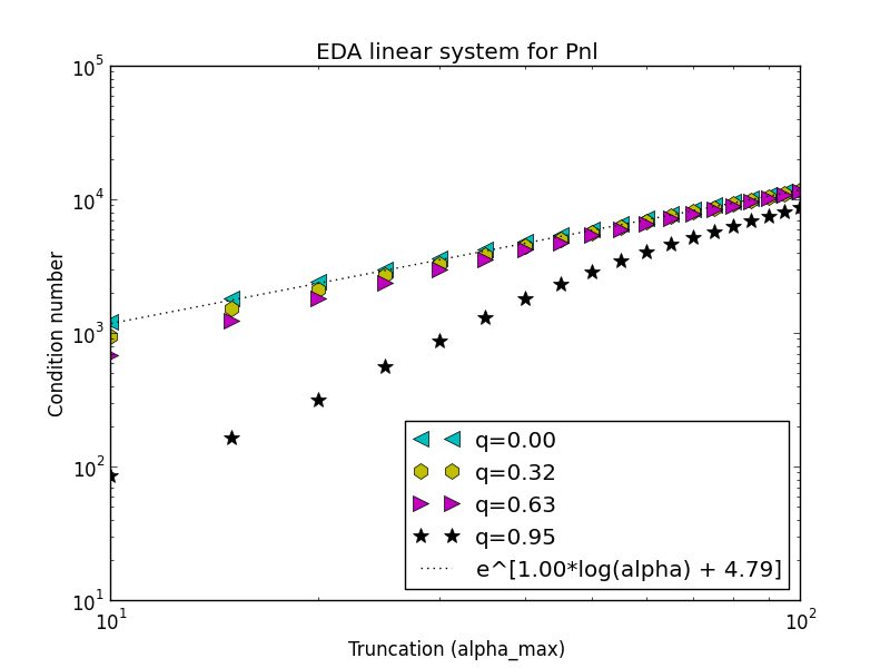
Figure 4: Log-log plot of the condition number $\kappa(A)$ for $\alpha_{\max}$ varying between $10$ and $100$, $\rho=0.95$, and different values of $q$. The curve slope for $q=0.0$ is $1.0$.

5 Conclusions

In this paper we have addressed a single-server queueing system with deterministic service time and exponentially delayed arrivals. The point process describing these arrivals dates back to the ’50s of the past century and was studied by Kendall and others.

We have described the model as a bivariate Markov chain, proved that the latter is ergodic, wrote the balance equations of the stationary distribution, and found a functional equation for the bivariate generating function. Then we have focused on the marginal distribution of the number of late customers and found its exact expression. This intermediate step has enabled the fundamental result on the super-exponential decay of the joint stationary distribution. The characterisation of the asymptotic behaviour has finally led us to show that the solution to the balance equations can be approximately computed in a simple yet very accurate way.

In spite of the big efforts we have put forward to find the solution to the functional equation (2.15), the complete solution of the problem is still out of reach. An expansion in powers of $q$ seems to be a promising approach to obtain (at least) an approximate expression of the bivariate generating function. This method allows to set up a recursive scheme to compute the coefficients of the power series, see [37, 49]. Unfortunately, the computations are quite involved and need some additional work to be refined. This will be the subject of further research and the topic of an upcoming paper.

Figures 2–5 were obtained using Python 2.7.9, numpy 1.9.1, scipy 0.15.1 matplotlib 1.4.2, and mpmath 0.19. The code to generate them is freely available on GitHub at the following address: https://github.com/clancia/EDA.

Appendix A Map of the quarter plane onto non-negative integers

Define the map $F$ of the quarter plane onto the set of the non-negative integers and its inverse $G$:

$$F(n,l)\mapsto m={n+l\choose 2}+l\,,$$

$$g(m)=\max\left\{j\geq 0\text{ such that }{j+1\choose 2}\leq m\right\}=\left\lfloor\frac{-1+\sqrt{1+8m}}{2}\right\rfloor\,,$$

$$G(m)=\left(g(m),m-g(m)\right)\,,$$

where $\left\lfloor\cdot\right\rfloor$ denotes the lower integer part, i. e. the floor operation. Fixed a positive integer $\alpha_{\max}$, let $k_{\max}={\alpha_{\max}+1\choose 2}$. Define the $k_{\max}\times k_{\max}$ matrix

$$A_{ij}=\begin{cases}\delta_{i,j}-\mathcal{P}(G(i),G(j))\,,&\quad i=0,1,\ldots,k_{\max}-1\,,\\ 1&\quad i=k_{\max}\,,\end{cases}$$ (A.1)

where $\mathcal{P}(\cdot,\cdot)$ is defined by (2.5)-(2.6), and

$$\pi_{j}=P_{g(j),j-g(j)}\,,\qquad j=0,1,\ldots,k_{\max}\,.$$ (A.2)

Remark 9.

The matrix (A.1) is rather sparse, as shown by Figure 5. We recommend to exploit this property by using sparse storage formats and dedicated libraries when $q$ is set larger than $0.98$. In this regime $\alpha_{\max}=100$ could be no longer sufficient to achieve a good approximation of $P_{n,l}$, but enlarging $\alpha_{\max}$ while using dense formats could quickly lead to memory shortage and a severe computational slowdown.

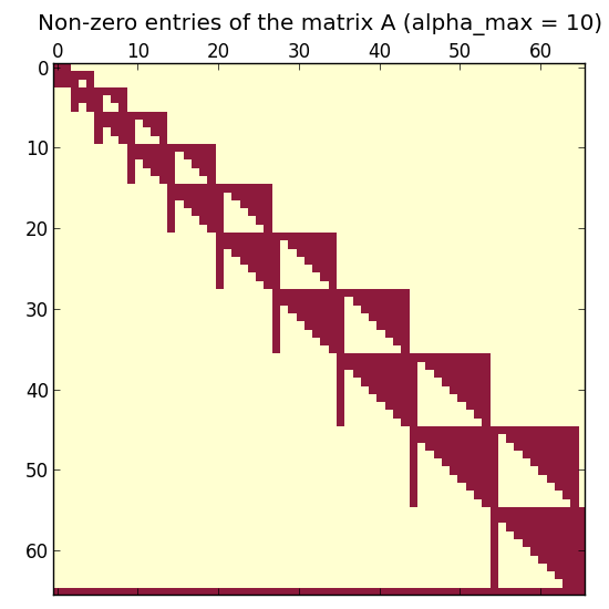
Figure 5: Sparsity structure of the matrix $A$, non-zero elements in dark colour ($\alpha_{\max}$ is set to $10$ for readability).

Appendix B Truncated System

By product of (3.14) and direct inspection of (2.5)–(2.6), for $i+j=\alpha_{\max}$,

$$\sum_{\begin{subarray}{c}n,l\geq 0\\ n+l>\alpha_{\text{\tiny max}}\end{subarray}}P_{n,l}\,\mathcal{P}((n,l),(i,j))\leq(1-\rho)\frac{(-q;q)_{\infty}}{(q;q)_{\infty}}\rho^{\alpha_{\text{\tiny max}}+1}q^{{\alpha_{\text{\tiny max}}+1\choose 2}}\,,$$ (B.1)

while for $i+j<\alpha_{\max}$,

$$\sum_{\begin{subarray}{c}n,l\geq 0\\ n+l>\alpha_{\text{\tiny max}}\end{subarray}}P_{n,l}\,\mathcal{P}((n,l),(i,j))=0\,,$$ (B.2)

where $P_{n,l}$ and $\mathcal{P}(\cdot,\cdot)$ are defined by (2.5)–(2.6) and (2.13), respectively. Also,

$$\sum_{\begin{subarray}{c}n,l\geq 0\\ n+l>\alpha_{\text{\tiny max}}\end{subarray}}P_{n,l}\leq 2\frac{(-q;q)_{\infty}}{(q;q)_{\infty}}\rho^{\alpha_{\text{\tiny max}}+1}q^{{\alpha_{\text{\tiny max}}+1\choose 2}}\,.$$ (B.3)

References

- [1] I. Adan, A. Economou, and S. Kapodistria, Synchronized reneging in queueing systems with vacations, Queueing Systems, 62 (2009), pp. 1–33.
- [2] I. Adan and V. Kulkarni, Single-server queue with Markov-dependent inter-arrival and service times, Queueing Systems, 45 (2003), pp. 113–134.
- [3] I. Adan, J. Wessels, and W. Zijm, A compensation approach for two-dimensional Markov processes, Advances in Applied Probability, (1993), pp. 783–817.
- [4] L. Ahlfors, Complex Analysis, an Introduction to the Theory of Analytic Functions of One Complex Variable, McGraw-Hill Book Company, 1953.
- [5] O. Almaz and T. Altiok, Simulation modeling of the vessel traffic in Delaware River: Impact of deepening on port performance, Simulation Modelling Practice and Theory, 22 (2012), pp. 146–165.
- [6] E. Altman and U. Yechiali, Analysis of customers’ impatience in queues with server vacations, Queueing Systems, 52 (2006), pp. 261–279.
- [7] G. Andrews, The theory of partitions, Cambridge University Press, 1998.
- [8] J. Artalejo, A. Economou, and M. Lopez-Herrero, Evaluating growth measures in an immigration process subject to binomial and geometric catastrophes., Mathematical biosciences and engineering: MBE, 4 (2007), p. 573.
- [9] S. Asmussen and O. Kella, A multi-dimensional martingale for Markov additive processes and its applications, Advances in Applied Probability, 32 (2000), pp. 376–393.
- [10] N. Bailey, A study of queues and appointment systems in hospital out-patient departments, with special reference to waiting-times, Journal of the Royal Statistical Society. Series B (Methodological), (1952), pp. 185–199.
- [11] M. Ball, T. Vossen, and R. Hoffman, Analysis of demand uncertainty effects in ground delay programs, in 4th USA/Europe Air Traffic Management R&D Seminar, 2001, pp. 51–60.
- [12] D. Bini, G. Latouche, and B. Meini, Numerical methods for structured Markov chains, Oxford University Press, 2005.
- [13] J. Blanc, A numerical study of a coupled processor model, University of Limburg, 1987.
- [14] , On a numerical method for calculating state probabilities for queueing systems with more than one waiting line, Journal of Computational and Applied Mathematics, 20 (1987), pp. 119–125.
- [15] P. Bloomfield and D. Cox, A low traffic approximation for queues, Journal of Applied Probability, (1972), pp. 832–840.
- [16] P. Brockwell, J. Gani, and S. Resnick, Birth, immigration and catastrophe processes, Advances in Applied Probability, (1982), pp. 709–731.
- [17] M. Caccavale, A. Iovanella, C. Lancia, G. Lulli, and B. Scoppola, A model of inbound air traffic: The application to Heathrow airport, Journal of Air Transport Management, 34 (2014), pp. 116–122.
- [18] T. Cayirli and E. Veral, Outpatient scheduling in health care: a review of literature, Production and Operations Management, 12 (2003), pp. 519–549.
- [19] J. Cohen, Boundary value problems in queueing theory, Queueing Systems, 3 (1988), pp. 97–128.
- [20] J. Cohen and O. Boxma, Boundary value problems in queueing system analysis, vol. 79, North Holland, 1983.
- [21] P. Collings, Limit theorems for processes of randomly displaced regular events, Journal of Applied Probability, (1976), pp. 530–537.
- [22] M. Combé and O. J. Boxma, BMAP modelling of a correlated queue, Network performance modeling and simulation, (1998), pp. 177–196.
- [23] C. Daganzo, The productivity of multipurpose seaport terminals, Transportation Science, 24 (1990), pp. 205–216.
- [24] Z. Drezner, On a queue with correlated arrivals, Journal of Applied Mathematics and Decision Sciences, 3 (1999).
- [25] A. Economou, The compound poisson immigration process subject to binomial catastrophes, Journal of Applied Probability, 41 (2004), pp. 508–523.
- [26] A. Economou and S. Kapodistria, q-Series in Markov chains with binomial transitions, Probability in the Engineering and Informational Sciences, 23 (2009), p. 75.
- [27] A. Economou, S. Kapodistria, and J. Resing, The single server queue with synchronized services, Stochastic Models, 26 (2010), pp. 617–648.
- [28] E. Edmond, Operation capacity of container berths for scheduled service by queuing theory, Dock Harbor Authority, 56 (1975), pp. 230–234.
- [29] G. Fayolle and R. Iasnogorodski, Two coupled processors: the reduction to a Riemann-Hilbert problem, Probability Theory and Related Fields, 47 (1979), pp. 325–351.
- [30] G. Fayolle, R. Iasnogorodski, and V. Malyshev, Random walks in the quarter-plane: algebraic methods, boundary value problems and applications, vol. 40, Springer, 1999.
- [31] H. Gail, S. L. Hantler, and B. Taylor, Use of characteristic roots for solving infinite state Markov chains, Computational Probability, (2000), pp. 205–255.
- [32] G. Gasper and M. Rahman, Basic hypergeometric series, vol. 96, Cambridge University Press, 2004.
- [33] G. Golub and W. Kahan, Calculating the singular values and pseudo-inverse of a matrix, Journal of the Society for Industrial & Applied Mathematics, Series B: Numerical Analysis, 2 (1965), pp. 205–224.
- [34] G. H. Golub and C. F. Van Loan, Matrix computations, John Hopkins University Press, 4th ed., 2012.
- [35] L. Govier and T. Lewis, Stock levels generated by a controlled-variability arrival process, Operations Research, 11 (1963), pp. 693–701.
- [36] W. Grassmann, Real eigenvalues of certain tridiagonal matrix polynomials, with queueing applications, Linear Algebra and its Applications, 342 (2002), pp. 93–106.
- [37] G. Guadagni, C. Lancia, S. Ndreca, and B. Scoppola, Queues with exponentially delayed arrivals, arXiv preprint at http://arxiv.org/abs/1302.1999v2, (2013).
- [38] G. Guadagni, S. Ndreca, and B. Scoppola, Queueing systems with pre-scheduled random arrivals, Mathematical Methods of Operations Research, 73 (2011), pp. 1–18.
- [39] C. Gwiggner and S. Nagaoka, Analysis of fuel efficiency in highly congested arrival flows, in Electronic Navigation Research Institute, Asia-Pacific International Symposium on Aerospace Technology, Tokyo-Japan, 2010.
- [40] G. Hardy and E. Wright, An introduction to the theory of numbers, Oxford University Press, 1979.
- [41] G. Hooghiemstra, M. Keane, and S. Van De Ree, Power series for stationary distributions of coupled processor models, SIAM Journal on Applied Mathematics, 48 (1988), pp. 1159–1166.
- [42] A. Iovanella, B. Scoppola, S. Pozzi, and A. Tedeschi, The Impact of 4D Trajectories on Arrival Delays in Mixed Traffic Scenarios, in Proceedings of the SESAR Innovation Days, D. Schaefer, ed., 2011.
- [43] D. Jagerman and T. Altiok, Vessel arrival process and queueing in marine ports handling bulk materials, Queueing Systems, 45 (2003), pp. 223–243.
- [44] C. Johnson, A gersgorin-type lower bound for the smallest singular value, Linear Algebra and its Applications, 112 (1989), pp. 1–7.
- [45] S. Kapodistria, The M/M/1 queue with synchronized abandonments, Queueing Systems, 68 (2011), pp. 79–109.
- [46] D. Kendall, Some recent work and further problems in the theory of queues, Theory of Probability & Its Applications, 9 (1964), pp. 1–13.
- [47] J. Kingman, Two similar queues in parallel, The Annals of Mathematical Statistics, 32 (1961), pp. 1314–1323.
- [48] G. Koole, On the use of the power series algorithm for general Markov processes, with an application to a Petri net, INFORMS Journal on Computing, 9 (1997), pp. 51–56.
- [49] C. Lancia, Looking through the cutoff window, PhD thesis, Technische Universiteit Eindhoven, 2013.
- [50] C. Lancia and G. Lulli, Data-driven modelling and validation of aircraft inbound-flow at some major european airports, In preparation, (2017).
- [51] G. Latouche and V. Ramaswami, Introduction to Matrix Geometric Methods in Stochastic Modeling, ASA-SIAM Series on Statistics and Applied Probability. SIAM, Philadelphia PA, 1999.
- [52] D. Lucantoni, New results on the single server queue with a batch Markovian arrival process, Stochastic Models, 7 (1991), pp. 1–46.
- [53] A. Mercer, A queueing problem in which arrival times of the customers are scheduled, Journal of the Royal Statistical Society Series B (Methodological), 22 (1960), pp. 108–113.
- [54] , Queues with scheduled arrivals: A correction, simplification and extension, Journal of the Royal Statistical Society. Series B (Methodological), (1973), pp. 104–116.
- [55] I. Mitrani and R. Chakka, Spectral expansion solution for a class of Markov models: Application and comparison with the matrix-geometric method, Performance Evaluation, 23 (1995), pp. 241–260.
- [56] R. Nelsen and T. Williams, Random displacements of regularly spaced events, Journal of Applied Probability, (1970), pp. 183–195.
- [57] M. Neuts, Structured stochastic matrices of M/G/1 type and their applications, vol. 701, Marcel Dekker New York, 1989.
- [58] , An interesting random walk on the non-negative integers, Journal of Applied Probability, (1994), pp. 48–58.
- [59] , Matrix-geometric solutions in stochastic models: an algorithmic approach, Dover Publications, 1995.
- [60] T. Nikoleris and M. Hansen, Queueing models for trajectory-based aircraft operations, Transportation Science, (2012).
- [61] A. Pacheco, N. Prabhu, and L. Tang, Markov-modulated processes & semiregenerative phenomena, World Scientific, 2009.
- [62] L. Qi, Some simple estimates for singular values of a matrix, Linear Algebra and Its Applications, 56 (1984), pp. 105–119.
- [63] P. Robert, Stochastic networks and queues, Springer-Verlag, 2003.
- [64] F. Sabria and C. Daganzo, Approximate expressions for queueing systems with scheduled arrivals and established service order, Transportation Science, 23 (1989), pp. 159–165.
- [65] H. Tijms, Stochastic models: an algorithmic approach, vol. 303, John Wiley & Sons Inc, 1994.
- [66] C. Winsten, Geometric distributions in the theory of queues, Journal of the Royal Statistical Society. Series B (Methodological), (1959), pp. 1–35.
- [67] S. Wittevrongel and H. Bruneel, Discrete-time queues with correlated arrivals and constant service times, Computers and Operations Research, 26 (1999), pp. 93–108.
- [68] A. Yaglom and I. Yaglom, Challenging mathematical problems with elementary solutions: Combinatorial analysis and probability theory, Dover Publications, 1964.
- [69] U. Yechiali, Queues with system disasters and impatient customers when system is down, Queueing Systems, 56 (2007), pp. 195–202.