Heterotic Mini-landscape in blow-up

Abstract

Localization properties of fields in compact extra dimensions are crucial ingredients for string model building, particularly in the framework of orbifold compactifications. Realistic models often require a slight deviation from the orbifold point, that can be analyzed using field theoretic methods considering (singlet) fields with nontrivial vacuum expectation values. Some of these fields correspond to blow–up modes that represent the resolution of orbifold singularities. Improving on previous analyses we give here an explicit example of the blow–up of a model from the heterotic Mini–landscape. An exact identification of the blow–up modes at various fixed points and fixed tori with orbifold twisted fields is given. We match the massless spectra and identify the blow–up modes as non–universal axions of compactified string theory. We stress the important role of the Green–Schwarz anomaly polynomial for the description of the resolution of orbifold singularities.

1 Introduction

Heterotic orbifolds are a fertile region of the string landscape (Lebedev:2006kn, ) in which the Minimal Supersymmetric Standard Model and Grand Unification Theories are widely encountered. They possess appealing features such as the existence of fixed sets (fixed points and fixed tori) where twisted states are localized. Those fixed sets yield quotient space singularities. Their properties depend on the action of the local subgroup of the orbifold group which leaves the particular set fixed. This locality can cause interesting physics (Forste:2004ie, ; Kobayashi:2004ya, ; Buchmuller:2004hv, ; Buchmuller:2005jr, ) and has lead to the concept of local grand unification (Nilles:2009yd, ; Nilles:2008gq, ; Buchmuller:2005sh, ) that has served to explore many promising models. Heterotic orbifolds give rise to discrete symmetries (Kobayashi:2006wq, ; CKMPZS, ), which explain the hierarchy between the electroweak and the unification scale (Kappl:2008ie, ), avoid proton decay (Forste:2010pf, ; Lee:2010gv, ), give rise to flavor symmetries (Ko:2007dz, ) and suppress the problematic $\mu$ term (Casas:1992mk, ; Antoniadis:1994hg, ; Lebedev:2007hv, ).

On the other hand the biggest set of heterotic string compactifications preserving $\mathcal{N}=1$ supersymmetry in 4d are the so called Calabi–Yau (CY) manifolds. The moduli space of the metric in Calabi–Yau manifolds consists of the complex structure moduli and the complexified Kähler structure moduli. There are well studied examples in which twisted states of orbifold models, which acquire vevs, smooth the singularities and can be identified with the moduli of the CY manifold (Hamidi:1986vh, ). This is expected because both CY and orbifold compactifications preserve $\mathcal{N}=1$ supersymmetry. In fact, all $T^{6}/\mathbb{Z}_{n}$ orbifolds are singular limits of smooth CY manifolds (Candelas:1985en, ; Hamidi:1986vh, ; Erler:1992ki, ; Aspinwall:1994ev, ; Reffert:2006du, ; Lust:2006zh, ; Nibbelink:2007rd, ; Nibbelink:2007pn, ). In the last years there has been an intense work in understanding the transition of the heterotic string compactified on those two geometries. For the string on orbifolds the conformal field theory is exactly solvable and all interactions explicitly computable. In contrast on a smooth CY the metric is not known and one has to rely on the topological information. In general one can not solve the conformal field theory, with the exception of certain points in the moduli space where a rational CFT description is available e.g. at the Gepner points. The way to proceed is to compactify the effective 10d $\mathcal{N}=1$ super Yang Mills coupled to supergravity on the CY. In this frame the index theorems (Witten:1981me, ; Witten:1984dg, ) determine the 4d massless fermionic chiral asymmetry.

There are physical motivations to deform away from the orbifold point in moduli space. At this point there are many exotics states, additional $U(1)$ symmetries and enhanced discrete symmetries. This differs from what is found in the real world and spontaneous symmetry breaking with vevs of twisted fields can give rise to much more realistic vacua. This breaking decouples exotics from the spectrum, reduces the abelian gauge sector and breaks partially global discrete symmetries. The partial breaking of discrete symmetries can be useful to create scale hierarchy, as the one needed for the pattern of quarks and leptons masses through a Froggatt–Nielsen mechanism (Froggatt:1978nt, ). In addition on the orbifold there exists an anomalous $U(1)_{A}$ symmetry which generates a Fayet–Iliopoulos D–term (FI), which breaks supersymmetry and can be cancelled by the vevs of twisted fields (Atick:1987gy, ; Dine:1987xk, ; Font:1988mm, ). The twisted fields which attain vevs can correspond to moduli of the CY geometry, which vanish at the orbifold point. At the orbifold point, the full spectrum, the interactions and the discrete symmetries can be determined. Thus, this connection can be used to extract information not known in the CY (Ludeling:2012cu, ).

The techniques of algebraic geometry in toric varieties (Oda, ; Fulton, ; Hori:2003ic, ) have been applied to make the orbifold singularities smooth (Erler:1992ki, ; Aspinwall:1994ev, ; Lust:2006zh, ; Nibbelink:2007rd, ; Nibbelink:2007pn, ). This process of removing the singularity and adding exceptional divisors of finite size $\text{Vol}(E_{r})$ is called blow–up or resolution, the inverse process is called blow–down. In the work (Nibbelink:2007rd, ) non–compact orbifolds singularities $\mathbb{C}^{3}/\mathbb{Z}_{N}$ as background of the heterotic superstring were resolved. In these models an abelian gauge flux in 6d is turned on. It is parametrized by vectors with indices in the $E_{8}\times E_{8}$ Cartan subalgebra which determine the field strength of a holomorphic vector bundle. In the blow–down limit these vectors correspond to shifts on the gauge degrees of freedom of the local orbifold action. Then, if we want to identify the heterotic orbifold as the singular limit of the CY, it is necessary to construct the vector bundle in such a way that orbifold rotations on the gauge degrees of freedom (d.o.f) are reproduced in the blow–down limit. For the compact cases in which there are different local singularities, the blow–down of local resolutions fixes the vector bundle such that it reproduces the local shifts (Nibbelink:2008tv, ; Nibbelink:2009sp, ).

The blow–up can be identified with the process of giving vevs to twisted fields. Using an exponential redefinition those twisted fields are interpreted as the CY Kähler moduli. This observation relies on the realization of the gauge transformation (Nibbelink:2009sp, ) and on the fact that the Kähler moduli are local, measuring the complex volume of the new cycles. Furthermore, a way of identifying those blow–up modes on the orbifold with the components of the vector bundle was proposed. This is based on the fact that the Bianchi Identities (BI) giving a consistent gauge flux, possess strong similarities with the mass equations of the orbifold states. In the gauged linear sigma model description (NibbelinkGroot:2010wm, ) the mass equation appears as the anomaly cancellation condition (Blaszczyk:2011ib, ; Blaszczyk:2011hs, ). Those results, opened a way to study the transition in a more precise manner. If both, the string theory on the blow–up geometry and the orbifold with vevs are coincident, then the massless spectrum should be identified.

In describing the departure from the orbifold point within realistic compact orbifolds (Nibbelink:2009sp, ; Blaszczyk:2010db, ; Buchmuller:2012mu, ) some difficulties were encountered in the $\mathbbm{Z}_{6II}$ Mini–Landscape (Lebedev:2006kn, ; Lebedev:2007hv, ; Lebedev:2008un, ) and the $\mathbbm{Z}_{2}\times\mathbbm{Z}_{2}$ Blaszczyk model of (Blaszczyk:2009in, ). The problems have two sources. One is the absence of a unique way to perform the toric resolution. In fact, there are many different resolutions connected by flop transitions (Blaszczyk:2010db, ). The second issue is the existence of discrete torsion (Vafa:1994rv, ; Ploger:2007iq, ), which allows for brother models and creates a further ambiguity in the identification. This occurs because the identification of the vector bundle with the local orbifold shift is only up to lattice vectors. In this work we are able to overcome those difficulties.

A complementary approach to explore the transition was proposed in (Nibbelink:2007ew, ). This method uses the fact that on the orbifold one encounters localized anomalies (Gmeiner:2002es, ) which depend on the chiral states at the fixed sets. On the blow–up, there exists also a localization on the cycles appearing in the resolution. Using the Green–Schwarz anomaly polynomial (Green:1984sg, ; Schellekens:1986xh, ) one can study the transition by comparing the anomaly in the blow–up and the anomaly on the orbifold deformed by vevs. At the first sight the anomaly cancellation mechanism seems very different in both cases. On the orbifold there is only one axion needed to cancel a universal anomaly whereas in the blow–up there are many anomalous $U(1)$s and many axions which cancel them. This can be explained by the change in the massless chiral spectrum, due to the field redefinitions and due to the fact that certain fields become massive in the blow–up. If the orbifold constitutes the blow–down limit of the toric CY, the anomaly polynomial encodes the complete information of that transition.

We look at the transition from the two sides. First we match the chiral massless spectrum. Using this identification we study the transition through the match of the anomaly cancellation in both regions of the moduli space. In a previous work, we studied the resolution of an MSSM like $T^{6}/\mathbb{Z}_{7}$ orbifold model (Blaszczyk:2011ig, ). This was simpler because all the exceptional divisors performing the resolutions are local, thus there is a local index theorem which allows to identify the spectrum. In addition there are no orbifold brother models, and there is a unique resolution for the local singularities (giving a unique resolution for the compact space). Nevertheless insights gained in that study apply in a modified way to our new situation.

Let us sketch now how the paper is structured. In section 2 we review the heterotic string on orbifolds and we present the $T^{6}/\mathbb{Z}_{6II}$ model that we chose as the key example. Section 3 is devoted to describe the orbifold toric resolution and the dimensional reduction of the $\mathcal{N}=1$ 10d theory on it. In section 4 we select the same resolution at all local $\mathbb{C}^{3}/\mathbb{Z}_{6II}$ singularities. We describe the Bianchi Identities and explain the search for blow–up modes among the orbifold twisted fields. As brother models are present we review the Mini–landscape models (Lebedev:2006kn, ; Lebedev:2007hv, ; Lebedev:2008un, ) to select an appropriate one. We have searched for candidates to blow–up modes among the twisted singlets. From this search we present one finding. In section 5 we discuss how field redefinitions are implemented to match the massless spectrum. In section 6 we study the matching for one set of blow–up modes. Imposing an agreement with orbifold mass terms, the allowed redefinitions are restrictive and we find one case in which the match works perfectly. In section 7, we study the anomaly cancelation in 4d, which constitutes an independent check of the picture. We compute the anomaly in the orbifold deformed by vevs and compare it with the dimensional reduction of the 10d anomaly on the resolution. We find agreement and local blow–up modes are identified as non–universal axions. The universal axion on the resolution turns out to be a mixture of the single orbifold axion and the blow–up modes. The check helps to establish the vacuum away from the orbifold as the CY manifold obtained by a resolution.

2 The Orbifold

In this section we review orbifold compactification of heterotic string theory. We then present the geometry of $T^{6}/\mathbb{Z}_{6II}$ and the heterotic orbifold model.

Heterotic string in orbifolds

The toroidal compactification of the 10d heterotic string leads to a four dimensional theory with $\mathcal{N}=4$ supersymmetry. It is possible to define a theory in which a symmetry of the toroidal lattice is modded out such that the 4d supersymmetry is reduced. This constitutes an orbifold compactification. Let us start with the six dimensional internal space and perform the toroidal compactification by identifying points under translations in a lattice $\Gamma_{6}$, to obtain $T^{6}=\mathbb{R}^{6}/\Gamma_{6}$. Now we take an isometry group $P$ of $\Gamma_{6}$, and perform a modding of this symmetry to get $T^{6}/P$, $P$ is called the point group. Modular invariance of the string partition function requires that the space group $S=\Gamma_{6}\rtimes P$ is embedded in the gauge degrees of freedom, we call this embedding $\mathfrak{g}$. Then the orbifold is defined by (Bailin:1999nk, )

$$\Omega=\mathbb{R}^{6}/(\Gamma_{6}\rtimes P)\times\Lambda/\mathfrak{g}.$$ (1)

In the bosonic representation of the gauge sector of the heterotic theory, $\Lambda=\Gamma_{8}\times\Gamma_{8}$ denotes the internal 16d torus. The heterotic worldsheet fields in the internal space are the bosonic space coordinates $X^{k}(z,\bar{z})$, the fermionic right–moving modes $\tilde{\psi}^{k}(\bar{z})$ and the 16d torus left–moving coordinates $X^{I}(z)$. The mentioned fields transform under the orbifold action as $X^{k}\rightarrow\theta^{kn}X^{n}+l^{k},\,k=5,...,10$, $\tilde{\psi}^{k}\rightarrow\theta^{kn}\tilde{\psi}^{n}$ and $X^{I}\rightarrow X^{I}+V^{I}+A^{I},I=1,...,16$, determining the twisted string boundary conditions.

Resuming, the orbifold action is given by $\theta\in P,\ \ l\in\Gamma_{6}$ and $V,A\in\mathfrak{g}$. The gauge embedding of the orbifold action is determined by $V$ and $A$, which represent the embedding of the spatial rotations $\theta$ and lattice translations $l$, respectively. The quantities $V$ and $A$ are refered to as shifts and Wilson lines respectively. Wilson lines turn out to be essential in order to break the gauge symmetry down to the Standard Model (Ibanez:1986tp, ). As there are six internal dimensions, vectors in the toroidal lattice $\Gamma_{6}$ can be expressed in terms of a basis $e_{\alpha},\,\alpha=1,...,6$, such that $l=n_{\alpha}e_{\alpha},\ \ A^{I}=n_{\alpha}A_{\alpha}^{I}$ $n_{\alpha}\in\mathbb{Z}$ , where $A_{\alpha}$ is the Wilson line corresponding to the lattice translation $e_{\alpha}$.

The space group  $S=\{(\theta,l)\}$ is defined as the subset of the orbifold (1) acting on the spatial internal dimensions $X^{k}$. Strings will propagate in the internal space given by $\mathbb{R}^{6}/S$. Worldsheet supersymmetry is preserved, because the twist commutes with the supersymmetry generator. This is ensured by the fact that the fermionic right–moving modes share the orbifold rotation. Furthermore, important objects are the fixed sets (fixed points and fixed tori) under the orbifold action. Those are defined by $X_{\mathbf{f}}=\theta X_{\mathbf{f}}+l$ where $X_{\mathbf{f}}$ are the 6d coordinates of the internal space. The space group element $(\theta,l)$ is called the constructing element of the fixed point (tori). Fixed points occur if $\det(1-\theta)\neq 0$. If the determinant vanishes we encounter fixed tori. For orbifolds generated by $\mathbb{Z}_{N}$ rotations that preserve the lattice $\Gamma_{6}$, take the orbifold action to be of the form

$$\theta=\exp(2\pi\text{i}(v_{1}J_{45}+v_{2}J_{67}+v_{3}J_{89})),\ \ \theta\in\mathbb{Z}_{N},$$ (2)

i.e. the transformation is block-diagonal in the internal part of the Lorentz group $SO(6)$. Here we denote the generators of rotations in the three distinct planes by $J_{45}$, $J_{67}$, $J_{89}$. We can impose that $\mathcal{N}=1$ supersymmetry survives the compactification. Then, the invariance of the susy algebra generators under the orbifold action yields the condition $\sum_{i}v_{i}=0$.

There is a beautiful conformal field theory description of orbifolds that we will not review here in detail (Dixon:1985jw, ; Dixon:1986jc, ; Dixon:1986qv, ). Essentially one solves the worldsheet equations of motion with the given boundary conditions and quantizes the string to obtain the twisted and untwisted oscillators. The physical states are obtained by acting with the latter on the twisted and untwisted vacua. Here we shortly present the ingredients required to compute the massless spectrum. Let us look at the states with boundary conditions given by the constructing element

$$g=\left(\theta^{k},m_{a}e_{a}\right)\in S.$$ (3)

The orbifold possesses untwisted and twisted modes which correspond to strings with boundary conditions $k=0$ and $k\neq 0$ respectively. The untwisted string states with constructing element $g=(1,0)$ can be described by $|q\rangle_{R}\otimes\tilde{\alpha}|p\rangle_{L}$. In that formula $q=(q^{0},q^{1},q^{2},q^{3})$ represents the momentum of the bosonized right–moving fermion. This is a weight of the $SO(8)$ Lorentz symmetry group which is manifest in the light cone gauge. The quantity $p$ denotes the left moving momentum of the 16 gauge d.o.f. and takes values in the $\Gamma_{8}\times\Gamma_{8}$ lattice, whereas $\tilde{\alpha}$ schematically denotes the set of left moving oscillators. The mass shell equations for massless states are given by

$$\frac{(p+V_{g})^{2}}{2}+N-1+\delta c=~{}\frac{(q+\phi_{g})^{2}}{2}-\frac{1}{2}+\delta c=0\,.$$ (4)

Here we have set the right oscillator numbers and the right–moving momentum to zero, to allow for massless right–movers. The phases $\phi_{g}=kv$ appearing in (4) are called local twists. $V_{g}$ represents the embedding on the gauge d.o.f. of the local constructing element $g$ in (3). The zero point energy is given by $\delta c=\frac{1}{2}\sum_{i=1}^{3}\omega_{i}(1-\omega_{i})$, with $\omega_{i}=(\phi_{g})_{i}\mod 1$ such that $0\leq\omega_{i}<1$ and the left–moving oscillator number is denoted by $N$. For twisted strings it is convenient to define the shifted left–moving momentum of the state as $P_{sh}=p+V_{g}$. The weight $P_{sh}$ determines the behavior of the twisted string under gauge transformations. An analogous definition is the shifted right–moving momentum $q_{sh}=q+v_{g}$. Then, twisted states with constructing element $g$ can be written as $|q_{sh}\rangle_{R}\otimes\tilde{\alpha}|P_{sh}\rangle_{L}$. They will transform under another space group element $h$ with a phase $[P_{sh}\cdot V_{h}-q_{sh}\cdot\phi_{h}-\frac{1}{2}(V_{g}\cdot V_{h}-\phi_{g}\cdot\phi_{h})]$. The surviving twisted spectrum is determined by imposing a trivial action under $h\in S$ if $[g,h]=0$. The surviving gauge group upon compactification is computed by determining the $E_{8}\times E_{8}$ roots $\alpha_{i}$ which fulfill $\alpha_{i}\cdot V=\alpha_{i}\cdot A_{\alpha}=0$.

The $T^{6}/\mathbb{Z}_{6II}$ model

In the work (Lebedev:2006kn, ) a large number of models of the $E_{8}\times E_{8}$ heterotic string compactified on $T^{6}/\mathbb{Z}_{6II}$ was studied. There, of the order of $100$ models with the spectrum of the MSSM were found. This Mini–landscape constitutes a fertile region of the space of $\mathcal{N}=1$ heterotic compactifications. The method they employed was to create models with local GUT gauge group at the fixed sets. The corresponding local GUTs had gauge groups $E_{6}$ and $SO(10)$. We focus on the models with $SO(10)$ local GUT. In those cases, the orbifold shift is chosen to break $E_{8}\times E_{8}$ down to $SO(10)$. Further breaking is performed by turning on the Wilson lines $A_{3}\equiv A_{4}$ and $A_{5}$. The torus lattice is the root lattice of $G_{2}\times SU(3)\times SO(4)$ and a basis for it can be found in (Nibbelink:2009sp, ).

In the Figures 1, 2 and 3 we depict the geometry of the $T^{6}/\mathbb{Z}_{6II}$ orbifold. The geometrical twist is given by $v=\{1/6,1/3,-1/2\}$. Let us denote the three complex coordinates by $z_{1},z_{2}$ and $z_{3}$, the twists acts on them as $\theta:z_{i}\rightarrow e^{2\pi iv_{i}}z_{i}$. The first figure corresponds to the first twisted sector $\theta$, which has 12 fixed points. We label the fixed points in the complex planes $i=1,2,3$ by $\alpha,\beta$ and $\gamma$ respectively, following the notation in (Nibbelink:2009sp, ). The Figure 2 corresponds to the fixed tori in the $\theta^{2}$ and $\theta^{4}$ sectors. In these sectors the plane $i=3$ is a fixed torus, so the twisted states will be localized at points in the first two planes and on a torus in the third. Fixed tori with $\alpha=3,5$ are identified under the orbifold, so we have 6 fixed tori in total. The $\theta^{3}$ sector is represented in Figure 3. In this case $z_{2}$ is fixed under rotations, which gives a torus in the second plane. In the first plane the fixed tori with $\alpha=2,4,6$ are identified on the orbifold. That gives us a total of 8 fixed tori. In Table 10 of Appendix A we give all the conjugacy classes of this orbifold with the corresponding fixed sets, together with the labels $\alpha,\beta$ and $\gamma$ denoting their loci in the three complex planes. Also the Coxeter element is given.

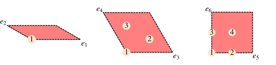
Figure 1: 12 fixed points of the $\theta$ sector from $T^{6}/\mathbb{Z}_{6II}$ orbifold. The labels of the fixed points in the planes 1, 2 and 3 denote $\alpha,\beta$ and $\gamma$, respectively.

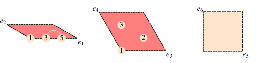
Figure 2: 6 fixed tori of the $\theta^{2}$ and $\theta^{4}$ sectors from $T^{6}/\mathbb{Z}_{6II}$ orbifold. The labels of the fixed points in the planes 1 and 2 denote $\alpha$ and $\beta$ respectively. Points $\alpha=3$ and $\alpha=5$ joined by a line are identified under a $\theta^{3}$ twist.

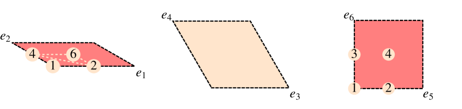
Figure 3: 8 fixed tori of the $\theta^{3}$ sector from $T^{6}/\mathbb{Z}_{6II}$ orbifold. The labels of the fixed points in the planes 1 and 3 denote $\alpha$ and $\gamma$ respectively. Points $\alpha=2,\,4,\,6$ joined by a line are identified under a $\theta^{2}$ twist.

We perform the study of the orbifold–resolution transition in Model 28 of the Mini–landscape. The shift and Wilson lines of that model are given by

$$V = \left(\frac{1}{3},-\frac{1}{2},-\frac{1}{2},0^{5},\frac{1}{2},-\frac{1}{6},-\frac{1}{2}^{5},\frac{1}{2}\right),$$ (5)

$$A_{5} = \left(-\frac{1}{2},-\frac{1}{2},0,\frac{1}{2},\frac{1}{2},0,0,0,\frac{15}{4},-\frac{19}{4},-\frac{15}{4},-\frac{15}{4},-\frac{15}{4},-\frac{15}{4},-\frac{11}{4},\frac{19}{4}\right),$$

$$A_{3} = A_{4}=\left(\frac{1}{6},\frac{1}{6},-\frac{1}{2},\frac{1}{6},\frac{1}{6},\frac{1}{6},\frac{1}{6},\frac{1}{6},\frac{5}{3},-\frac{2}{3},-\frac{5}{3},-\frac{5}{3},-\frac{5}{3},-\frac{5}{3},-\frac{1}{3},\frac{8}{3}\right).$$

The shift breaks $E_{8}\times E_{8}$ down to $SO(10)$. Adding the Wilson lines the gauge group is broken down further to $SU(3)\times SU(2)\times SU(6)\times U(1)^{8}$. A review of the non–Abelian charges of the spectrum is given in Table 1.

Table 1: Massless spectrum of the Mini–landscape Model 28. We give the representations under the non–abelian gauge group $SU(3)\times SU(2)\times SU(6)$ and the multiplicities of the states.

irrep.	$\mathbf{(1,1,1)}$	$\mathbf{(1,2,1)}$	$\mathbf{(3,1,1)}$	$\mathbf{(\bar{3},1,1)}$	$\mathbf{(1,1,6)}$	$\mathbf{(1,1,\bar{6})}$	$\mathbf{(3,2,1)}$	$\mathbf{(\bar{3},2,1)}$
mult.	114	19	22	16	7	7	1	4

3 Smoothing the singularities

In this section we describe how the spectrum is determined when compactifying the theory on the resolved space. We review the resolution process of the local singularities and give the relevant data for the geometry of the resolved space. Then we describe how the dimensional reduction of the 10d theory is performed.

The geometry

The local orbifold singularities are resolved and the resulting patches are joined to obtain a global resolution (Lust:2006zh, ). The local singularities at the fixed points of $\theta$ are $\mathbb{C}^{3}/\mathbb{Z}_{6II}$ singularities. Transversally to the fixed tori of $\theta^{2}$ and $\theta^{4}$ one has $\mathbb{C}^{2}/\mathbb{Z}_{3}$ singularities. Similarly for the fixed tori of $\theta^{3}$ the local singularities are $\mathbb{C}^{2}/\mathbb{Z}_{2}$.

Let $N_{\mathbb{R}}=\mathbb{N}^{r}\otimes\mathbb{R}$. A cone $\sigma\subset N_{\mathbb{R}}$ is a set $\sigma=\{a_{1}v_{1}+a_{2}v_{2}+...+a_{k}v_{k}|a_{i}\in\mathbb{R},\,a_{i}\geq 0\}$ generated by a finite set of vectors $v_{1},v_{2},...,v_{k}$ in $\mathbb{N}^{r}$ such that $\sigma\cap(-\sigma)=\{0\}$. A collection $\Sigma$ of cones in $N_{\mathbb{R}}$ is called a fan if each face of a cone in $\Sigma$ is also a cone in $\Sigma$ and the intersection of two cones in $\Sigma$ is a face of each of them.

Starting from a fan $\Sigma$ one can construct a toric variety $X$. The fans are spanned by vectors $v_{1},v_{2},...,v_{n}$ lying in the lattice $\mathbb{N}^{r}$. They define a complex toric variety $X$ of $\dim_{\mathbb{C}}(X)=n-r$, as the quotient of an open subset in $\mathbb{C}^{n}$ under a group $G$ as $X=(\mathbb{C}^{n}-Z(\Sigma))/G$. Let us denote the coordinates by $(z_{1},z_{2},...,z_{n})\in(\mathbb{C}^{n}-Z(\Sigma))$. The vectors $v_{i}$ represent divisors $z_{i}=0$. The group $G$ is defined as the kernel of the map

$$\phi:(\mathbb{C}^{*})^{n}\rightarrow(\mathbb{C}^{*})^{r},\ \ \ (t_{1},....,t_{n})\rightarrow(\prod_{j=1}^{n}t_{j}^{v_{j1}},...,\prod_{j=1}^{n}t_{j}^{v_{jr}}),$$ (6)

and acts on the coordinates $z_{i}$ as $t_{i}z_{i}$, where $t_{i}$ are the solutions to $(\prod_{j=1}^{n}t_{j}^{v_{j1}},...,\prod_{j=1}^{n}t_{j}^{v_{jr}})=(1,...,1)$. Fans describing the d–dim local toric singularities are defined by a d-1–dim simplex $S_{d-1}$ lying in a hyperplane at distance one from the origin in $N_{\mathbb{R}}$, so that all rays $av_{k},a\in\mathbb{R}^{+}$ go from the origin through $S_{d-1}$. $S_{d-1}$ and its triangulation is called toric diagram in the following. $Z(\Sigma)$ is an exclusion set encoded in the triangulation of the toric diagram (Hori:2003ic, ) and is given by the union of divisor intersections which do not span a cone in $\Sigma$. The variety is singular if not all the points in the lattice $\mathbb{N}^{r}$ can be written as a linear combination of the vectors $v_{i}$ with integer coefficients. Therefore, adding new vectors $\omega_{r}$ which subdivide the diagram is equivalent to resolving the variety.

The orbifold singularity $\mathbb{C}^{2}/\mathbb{Z}_{n}$ has a toric diagram given by $v_{1}=(1,0)$ and $v_{2}=(1,n)$, and the orbifold group $G=\{(t,t^{n-1}),\ \ t^{n}=1\}$ acts on $(z_{1},z_{2})$ as $(tz_{1},t^{n-1}z_{2})$. The divisors $D_{1}=\{z_{1}=0\}$ and $D_{2}=\{z_{2}=0\}$ correspond to the vectors $v_{1}$ and $v_{2}$. The blow–up is performed by subdividing the diagram. This is done by adding the vectors $\omega_{r}=(1,r),\ \ r=1,..,n-1$, which correspond to $n-1$ exceptional divisors $E_{r}=\{y_{r}=0\}$, where $y_{r}$ are new coordinates on the variety. In Figure 4, we give the diagrams for the resolution of the local singularities $\mathbb{C}^{2}/\mathbb{Z}_{3}$ and $\mathbb{C}^{2}/\mathbb{Z}_{2}$.

Figure 4: Resolutions of the local singularities under the $\theta^{3}$ and $\theta^{2},\theta^{4}$ action respectively.

$\mathbb{C}^{2}/\mathbb{Z}_{2}$	$\mathbb{C}^{2}/\mathbb{Z}_{3}$

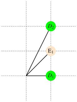
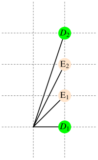
The resolved $\mathbb{C}^{2}/\mathbb{Z}_{2}$ has coordinates $(z_{1},z_{2},y_{1})$ identified under $G_{2}=\{(t,t,t^{-2}),t\in\mathbb{C}^{*}\}$. The exclusion set is $z_{1}=z_{2}=0$. The resolved $\mathbb{C}^{2}/\mathbb{Z}_{3}$ has coordinates $(z_{1},z_{2},y_{1},y_{2})$ identified under $G_{3}=\{(t_{1},t_{2},t_{1}^{-2}t_{2},t_{1}t_{2}^{-2}),t_{1},t_{2}\in\mathbb{C}^{*}\}$ with $Z(\Sigma)=(z_{1}=z_{2}=0)\cup(z_{1}=y_{2}=0)\cup(z_{2}=y_{1}=0)$.

Let us look at the local singularity $\mathbb{C}^{3}/\mathbb{Z}_{6II}$. In this case we have to add four new coordinates $y_{r}$ to the complex coordinates $z_{1},z_{2},z_{3}\in\mathbb{C}^{3}$ and four new scaling relations to define the smooth global variety. The kernel of $(t_{1},t_{2},t_{3},\tilde{t}_{1},...,\tilde{t}_{4})\rightarrow(\prod_{i,k}t^{(v_{i})_{1}}_{i}\tilde{t}^{(\omega_{k})_{1}}_{k},...,\prod_{i,k}t^{(v_{i})_{3}}_{i}\tilde{t}^{(\omega_{k})_{3}}_{k})$ defines the new $(\mathbb{C}^{*})^{4}$ action. Here $\omega_{k}=g_{i}v_{i}$, where $z_{i}$ goes to $e^{2\pi ig_{i}v_{i}}z_{i}$ under $\theta^{k}$ (Aspinwall:1994ev, ). Hence the new variety is defined by coordinates $(z_{1},z_{2},z_{3},y_{1},y_{2},y_{3},y_{4})$ identified under a $(\mathbb{C}^{*})^{4}$ action given by

$$G_{6}=\{(t_{4}^{-1/6}t_{5}^{1/3}t_{6}^{-1/2}t_{7}^{-2/3},t_{4}^{-1/3}t_{5}^{-2/3}t_{7}^{-1/3},t_{4}^{-1/2}t_{6}^{-1/2},t_{4},t_{5},t_{6},t_{7}),t_{4},t_{5},t_{6},t_{7}\in\mathbb{C}^{*}\}.$$

The $\mathcal{N}=1$ supersymmetry condition is equivalent to the Calabi–Yau condition. The latter is ensured if the added vectors resolving the singularity lie in the hyperplane defined by $v_{1}$, $v_{2}$ and $v_{3}$. The vectors $v_{i}$ and $\omega_{k}$ are associated with divisors $D_{i}=\{z_{i}=0\}$ and $E_{k}=\{y_{k}=0\}$, which are ordinary and exceptional divisors respectively. In the Figure 5 we draw the 2–simplices $S_{2}$ defining the five distinct toric resolutions of $\mathbb{C}^{3}/\mathbb{Z}_{6II}$.

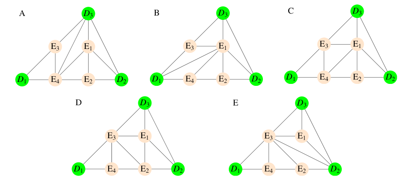
Figure 5: Local resolutions of the $\mathbb{C}^{3}/\mathbb{Z}_{6II}$ orbifold. There are five different ways of defining the fan (Oda, ) which are represented by the five possible triangulations of the 2–simplices. The divisor $E_{2}$ corresponding to $\omega_{2}$ has coordinates $(0,0,1)$. All $v_{i}$ are of the form $(*,*,1)$.

Those are given by the different triangulations of the toric diagram. The triangulation defines the value of $Z(\Sigma)$. For example triangulation B has $Z(\Sigma)=(y_{3}=y_{4}=0)\cup(y_{3}=y_{2}=0)$ $\cup(y_{3}=z_{2}=0)\cup(z_{1}=z_{3}=0)$ $\cup(z_{1}=z_{2}=0)\cup(z_{1}=y_{2}=0)$ $\cup(y_{4}=z_{2}=0)\cup(z_{3}=y_{4}=0)$ $\cup(z_{3}=y_{2}=0)$. Three divisors that correspond to the corners of a basic triangle have intersection 1. Triplets of divisors that do not have this property have intersection 0. Equivalence relations between the divisors are given by $\sum(v_{i})_{j}D_{i}+\sum_{k}(\omega_{k})_{j}E_{k}\sim 0$. Using Poincaré duality and Stokes theorem we relate cycles with closed–forms. Homology relations between the cycles translate into cohomology relations between the forms i.e. equivalences up to exact cycles translates into equivalences up to exact forms.

The global information is obtained by taking into account all local resolutions and including the inherited divisors $R_{i}$ which are the Poincaré duals of the (1,1) invariant orbifold forms $dz_{i}\wedge d\bar{z}_{\bar{i}}$. An auxiliary polyhedron obtained in (Reffert:2006du, ; Lust:2006zh, ) and employed in (Nibbelink:2009sp, ) encodes all the triple intersections. In that way, new cohomology classes arise in the blow–up and it is possible to determine topological information from them. Taking the volume of the resolution cycles to zero $\text{Vol}(E_{r})\rightarrow 0$ the geometrical orbifold is recovered.

Applying the method of the auxiliary polyhedra it is possible to determine the set of intersections for the compact resolved orbifold $\mathcal{M}=\widehat{T^{6}/\mathbb{Z}_{6II}}$. Triple intersections of distinct divisors belonging to local resolutions have the values that can be read from the local toric diagrams. On the $\widehat{T^{6}/\mathbb{Z}_{6II}}$ the divisors have indices corresponding to the fixed points from which they come. $D_{i,\rho}$ represents the ordinary divisor corresponding to the fixed point singularity $\rho$ in the complex plane $i$. There are in total 10 ordinary divisors $D_{1,1}$, $D_{1,2}$, $D_{1,3}$, $D_{2,\beta}$ and $D_{3,\gamma}$. The exceptional divisors $E_{1,\beta\gamma}$, $E_{2,\alpha\beta}$, $E_{4,\alpha\beta}$ and $E_{3,\alpha\gamma}$ have their first index denoting the sector and the two following indices denoting the corresponding fixed point singularity. The global equivalence relations (Nibbelink:2009sp, ) determine $D_{i,\rho}$ as linear combinations of $E_{r}$ and $R_{i}$. Using those equivalence relations for divisors it is possible to obtain the non–zero intersection numbers of exceptional divisors only. Those intersections are the ones used in performing the dimensional reduction of the 10d theory and are given by

$$E_{1,\beta\gamma}^{3} = 6,E_{2,1\beta}^{3}=8,E_{3,1\gamma}^{3}=8,E_{4,1\beta}^{3}=8,E_{1,\beta\gamma}E_{2,1\beta}^{2}=-2,$$ (7)

$$E_{1,\beta\gamma}E_{3,1\gamma}^{2} = -2,E_{1,\beta\gamma}E_{4,1\beta}^{2}=-2,E_{1,\beta\gamma}E_{2,1\beta}E_{4,1\beta}=1,E_{2,1\beta}^{2}E_{4,1\beta}=-2,$$

$$c_{2}(\mathcal{M})E_{2,1\beta} = c_{2}(\mathcal{M})E_{4,1\beta}=c_{2}(\mathcal{M})E_{3,1\gamma}=-4,\,\,c_{2}(\mathcal{M})R_{2}=c_{2}(\mathcal{M})R_{3}=24.$$

The second Chern–class of the manifold $c_{2}(\mathcal{M})$ is the piece of degree two in the formal variables $D_{J},E_{r}$ and $R_{i}$ in the total Chern–class (Nibbelink:2009sp, ) according to

$$c(\mathcal{M})=\prod_{J,r}(1+D_{J})(1+E_{r})(1-R_{1})(1-R_{2})(1-R_{3})^{2}.$$ (8)

Supergravity on the resolution

What is known about the geometry of $\widehat{T^{6}/\mathbb{Z}_{6II}}$ is mainly the topological information e.g. the set of intersection numbers between divisors. In order to determine the theory in 4d one can perform a dimensional reduction of the 10d $\mathcal{N}=1$ theory, which is supergravity coupled to super Yang–Mills. Massless 4d tensor fields descend from the 10d heterotic massless tensor fields by reducing the latter on harmonic forms in $\widehat{T^{6}/\mathbb{Z}_{6II}}$. Let us consider the descendants of the fields with representations $(\mathbf{35},\mathbf{1},\mathbf{1})$ and $(\mathbf{28},\mathbf{1},\mathbf{1})$ under $SO(8)\times E_{8}\times E_{8}$. Here $SO(8)$ is the Little group of the 10d Lorentz group for massless states and $E_{8}\times E_{8}$ is the gauge group of the heterotic string. The massless tensor and form fields in 10d are the metric $\mathfrak{G}$ and the antisymmetric Kalb–Ramond field $B_{2}$ of $SO(8)$ respectively. Their expansions in the base of the internal $(1,1)$ harmonic forms are (Nibbelink:2009sp, )

$$\mathfrak{G}=g+J=g+a_{i}R_{i}-b_{r}E_{r}\,,\qquad B_{2}=b_{2}+B=b_{2}+\alpha_{i}R_{i}-\beta_{r}E_{r}\,,$$ (9)

where $J$ is the Kähler form, $B$ is the internal 6d component of $B_{2}$, $b_{2}$ is the 4d component of $B_{2}$ and $g$ is the 4d component of the metric. In four dimensions $J$ and $B$ join to form the complex scalar components of the chiral multiplets $T_{i}|_{\theta=0}=a_{i}+i\alpha_{i}$ and $T_{r}|_{\theta=0}=b_{r}+i\beta_{r}$. The real components $a_{i},b_{r}$ govern the size of the $R_{i}$ and $E_{r}$ cycles, respectively. The four dimensional field $b_{2}$ is the dual of the blow–up universal axion $a^{\rm uni}$. Let us write the field strength $H_{3}$

$$H_{3}=dB_{2}-\Omega_{3}^{\rm YM}+\Omega_{3}^{\rm L}.$$ (10)

$\Omega_{3}^{\rm YM}$ and $\Omega_{3}^{\rm L}$ are the gauge and gravitational Chern–Simons 3–forms respectively (GSW2, ). The gauge invariance of $H_{3}$ under abelian gauge transformations with gauge parameter $\chi^{I}$ implies the following variations

$$\delta\beta_{r}=V^{I}_{r}\chi^{I},\ \ \ \ \delta\alpha_{i}=0,$$ (11)

of the dimensionally reduced antisymmetric tensor. The gauge variation of those axions cancels the 4d anomaly, which can be determined by dimensional reduction or direct evaluation (Blaszczyk:2011ig, ). It is precisely the gauge variation of the $\beta_{r}$ moduli that leads to the interpretation that the $\exp(\beta_{r})$ correspond to twisted orbifold states (Nibbelink:2009sp, ).

The corresponding blow–up model to a deformed orbifold has a gauge group determined by the breaking of the orbifold gauge group by the vevs of the blow–up modes. Thus, in the blow–up the $E_{8}\times E_{8}$ group should be broken. The 6d flux $\mathcal{F}$ which is required for consistency breaks $E_{8}\times E_{8}$ down to a subgroup. Consistency conditions restricting the flux are the zero supersymmetric variation of the gaugino giving the Donaldson Uhlenbeck Yau (DUY) theorem $\int_{\mathcal{M}}\text{tr}\mathcal{F}\wedge J\wedge J=0$ and the Bianchi Identities $\int_{S}dH=0$, for $S$ any compact divisor on the manifold $\mathcal{M}$. Abelian gauge fluxes satisfying the DUY theorem are the field strengths of holomorphic vector bundles. The Bianchi Identities are given by

$$0=\int\limits_{S}\left(\text{tr}\mathcal{R}^{2}-\text{tr}\mathcal{F}^{2}\right)\,,\qquad S\in\{E_{r},R_{i}\}\,.$$ (12)

The second Chern–class is related to the internal curvature by $\text{tr}\mathcal{R}^{2}=-2c_{2}(\widehat{T^{6}/\mathbb{Z}_{6II}})$. We consider an Abelian flux

$$\mathcal{F}=H_{I}V^{I}_{r}E_{r},$$ (13)

where $r$ runs over indices of the orbifold fixed sets, which are denoted by $(1,\beta,\gamma)$, $(2,\alpha,\beta)$, $(4,\alpha,\beta)$ and $(3,\alpha,\gamma)$. The first entry represents the twisted sector and the $\alpha,\beta$ and $\gamma$ indices the fixed point in the first, second and third plane. The $H_{I}$ are the Cartan generators of $E_{8}\times E_{8}$. The vectors $V^{I}_{r}$ determine the field strength of the vector bundle and are subject to the following constraints: they must satisfy flux quantization conditions which are fulfilled by requiring $V_{r}\sim V_{(\theta^{k},\lambda)}$, where $V_{(\theta^{k},\lambda)}$ is the local orbifold shift corresponding to the constructing element $(\theta^{k},\lambda)$ which coincides with $r$. Note that the above equivalence is up to lattice vectors. The $V_{r}$ also have to satisfy the Bianchi Identities (12), which constrain their lengths and scalar products.

The massless fermion fields whose reductions gives the 4d massless chiral matter are the 10d states $(\mathbf{8},\mathbf{248},\mathbf{1})$ and $(\mathbf{8},\mathbf{1},\mathbf{248})$ characterized by the $E_{8}\times E_{8}$ root vectors. Their 4d multiplicity is determined using an index theorem which detects the 4d fermionic chiral asymmetry (Witten:1984dg, ; GSW2, ). The multiplicity operator is given by

$$\hat{N}=\frac{1}{6}\int\limits_{\mathcal{M}}\left(\mathcal{F}^{3}-\frac{1}{4}\text{tr}\mathcal{R}^{2}\mathcal{F}\right)\,.$$ (14)

Upon dimensional reduction (14) defines with which multiplicity the states appear in the spectrum. The surviving gauge group is determined by all the $E_{8}\times E_{8}$ roots with fulfill $\alpha_{i}\cdot V_{r}=0$. This can be seen by dimensionally reducing the Yang–Mills action. The representation of a given state can be computed with the Dynkin labels, which are determined by the product $\alpha_{i}\cdot p$ between the surviving simple roots in 4d $\alpha_{i}$ and the root vector $p$ characterizing the state.

4 Identifying the blow–up modes

In this section we explain the search for blow–up modes using the Bianchi Identities on the resolved orbifold. We focus on the case in which all local fixed sets have the same resolution. The search for blow–up modes is performed among all twisted states of the Mini–landscape MSSM model. We start with an orbifold model in which localized chiral superfields appear at all the fixed sets. Then, we explore solutions of the Bianchi Identities, which correspond to massless non–oscillatory blow–up modes. In triangulation B there are multiple sets of modes which fulfill the Bianchi Identities and therefore multiple ways of blowing–up. They determine to which extent the hidden gauge group is broken. All of the encountered vacua possess moduli with different chirality in the orbifold theory. We find multiple solutions which correspond to massless and non oscillatory states, whose vevs preserve the hidden group.

We can fix the topology of the resolved manifold by specifying the triangulation at all local $\mathbb{C}^{3}/\mathbb{Z}_{6II}$ resolutions. Then, using the Bianchi Identities we search for consistent sets of vevs of the twisted fields. Let us describe as an example $\widehat{T^{6}/\mathbb{Z}_{6II}}$ were we chose at all fixed points triangulation B. This triangulation has the least non–vanishing self–intersections, and therefore leads to the least restrictive equations for the vectors $V_{r}$.

In $\widehat{T^{6}/\mathbb{Z}_{6II}}$ the abelian field strength of the vector bundle (13) is given by

$$\mathcal{F}=H_{I}\left(\sum_{\beta=1}^{3}\sum_{\gamma=1}^{4}V^{I}_{1,\beta\gamma}E_{1\beta\gamma}+\sum_{k=2,4}\sum_{\alpha=1,3}\sum_{\beta=1}^{3}V^{I}_{k,\alpha\beta}E_{k\alpha\beta}+\sum_{\alpha=1}^{2}\sum_{\gamma=1}^{4}V^{I}_{3,\alpha\gamma}E_{3\alpha\gamma}\right).$$ (15)

To obtain the Bianchi Identities (12) and the multiplicity of the massless states in blow–up we need all the self intersections of exceptional divisors in equation (7). The multiplicity of a state with $E_{8}\times E_{8}$ weight $\omega$ can be written as

$$\hat{N} = \sum_{\beta\gamma}\hat{N}_{1,\beta\gamma}(\omega)+\sum_{\beta}\hat{N}_{2,\beta}(w)+\sum_{\gamma}\hat{N}_{3,\gamma}(\omega),$$ (16)

$$\hat{N}_{1,\beta\gamma}(\omega) = -V_{1,\beta\gamma}\cdot\omega\left((V_{2,1\beta}\cdot w)^{2}+(V_{4,1\beta}\cdot\omega)^{2}-(V_{2,1\beta}\cdot w)(V_{4,1\beta}.\omega)-(V_{1,\beta\gamma}\cdot\omega)^{2}+(V_{3,1\gamma}\cdot\omega)^{2}\right),$$

$$\hat{N}_{2,\beta}(w) = \frac{1}{3}\left(4(V_{2,1\beta}\cdot\omega)^{3}+4(V_{4,1\beta}\cdot\omega)^{3}-V_{2,1\beta}\cdot\omega-V_{4,1\beta}\cdot\omega-3(V_{2,1\beta}\cdot\omega)^{2}(V_{4,1\beta}\cdot\omega)\right),$$

$$\hat{N}_{3,\gamma}(\omega) = \frac{1}{3}\left(4(V_{3,1\gamma}\cdot\omega)^{3}-V_{3,1\gamma}\cdot\omega\right).$$

Using (7) the Bianchi Identities (12) give rise to the formulas

$$24-\sum_{\gamma}V^{2}_{3,1\gamma}-3\sum_{\gamma}V^{2}_{3,2\gamma}=0,$$ (17)

$$3V^{2}_{1,\beta\gamma}-(V_{2,1\beta};V_{4,1\beta})-V^{2}_{3,1\gamma}=0,$$ (18)

$$-2-V_{3,1\gamma}\cdot\sum_{\beta}V_{1,\beta\gamma}+2V^{2}_{3,1\gamma}=0,$$ (19)

$$24-\sum_{\beta}(V_{2,1\beta};V_{4,1\beta})-2\sum_{\beta}(V_{2,3\beta};V_{4,3\beta})=0,$$ (20)

$$-12-3V_{4,1\beta}\cdot\sum_{\gamma}V_{1,\beta\gamma}+6V^{2}_{4,1\beta}+2(V_{2,1\beta};V_{4,1\beta})=0,$$ (21)

$$-12-3V_{2,1\beta}\cdot\sum_{\gamma}V_{1,\beta\gamma}+3V^{2}_{4,1\beta}+4(V_{2,1\beta};V_{4,1\beta})=0,$$ (22)

for triangulation B in all local $\mathbb{C}^{3}/\mathbb{Z}_{6II}$ resolutions. We use the notation $(V_{1};V_{2})=V_{1}^{2}+V_{2}^{2}-V_{1}\cdot V_{2}$. This set of equations allows us to explore if a given orbifold model has candidates for blow–up modes fulfilling the Bianchi Identities, which are conjectured to be linked to the orbifold mass equations (Nibbelink:2009sp, ; Blaszczyk:2011ib, ; Blaszczyk:2011hs, ). This exploration can be performed in a reasonable computing time. We take the orbifold Model 28 of the Mini–landscape. The equation (17) is automatically satisfied for all the corresponding states in the considered model and they are also satisfied for the Mini–landscape model discussed in (Nibbelink:2009sp, ).

The equations (17) involving $V_{3,\alpha\gamma}$ are automatically satisfied because in all the fixed tori $(3,\alpha,\gamma)$ the singlets surviving the orbifold projection fulfill $P_{sh}^{2}=V^{2}_{3,\alpha\gamma}=\frac{3}{2}$, i.e. have zero oscillator number.

Let us describe here the further steps of the exploration for triangulation B. First, for given values of $V_{3,\alpha\gamma}$, we select all the $V_{1,\beta\gamma}$ which obey (19). For a fixed $V_{3,\alpha\gamma}$ there are $2401$ possibilities for $V_{1,\beta\gamma}$. There are $50400$ $V_{2,\alpha\beta}$ and $V_{4,\alpha\beta}$ that satisfy (20). From this surviving set we explore which $V_{1,\beta\gamma},V_{2,\alpha\beta},V_{4,\alpha\beta}$ satisfy the equations (18) (21) and (22), which turn to be the hardest to obey. An exploration for a fixed $V_{3,\alpha\gamma}$ requires $1.2\times 10^{8}$ iterations, while a full exploration will require of the order of $3\times 10^{10}$ iterations. In the exploration we performed, we found multiple sets of blow–up modes which can be identified with twisted states of Model 28.

The blow–up modes identified with twisted fields have to acquire vevs to ensure D-flatness and F-flatness of the superpotential. The local shift of the blow–up modes $P_{sh}\equiv V_{r}$ satisfy the Bianchi Identities of the vector bundle (Nibbelink:2009sp, ). In the following we give the simplified Bianchi Identities for triangulation B and one of the encountered solutions.

Abelian vector bundles for triangulation B

Now we come to the solutions of the Bianchi Identities for triangulation B. Considering massless and non–oscillatory modes, the equations (17)-(22) are given by

$$(V_{2,1\beta};V_{4;1\beta})=\frac{8}{3},$$ (23)

$$\sum_{\beta}(V_{2,3\beta};V_{4,3\beta})=8,$$ (24)

$$V_{3,1\gamma}\cdot\sum_{\beta}V_{1,\beta\gamma}=1,$$ (25)

$$V_{4,1\beta}\cdot\sum_{\gamma}V_{1,\beta\gamma}=\frac{8}{9},$$ (26)

$$V_{2,1\beta}\cdot\sum_{\gamma}V_{1,\beta\gamma}=\frac{10}{9}.$$ (27)

We found sets of blow–up modes which can either break or preserve the hidden group. We also explored the possibility to obtain certain chirality features for a set of blow–up modes. The fact that the modes in sectors $\theta^{2}$ and $\theta^{4}$ are CPT conjugate to each other is incompatible with having modes that are massless and non–oscillatory in both the $\theta$ and $\theta^{3}$ sectors. A possibility would be that in the $\theta^{2}$ sector all the modes are left handed and in the $\theta^{4}$ sector all are right handed, but this can not be achieved in our case. For example in the case of $V_{2,11}$ and $V_{4,11}$ the only opposite chirality modes are $V_{2,11}=-V_{4,11}$ and this implies $(V_{2,11};V_{2,11})=\frac{14}{3}$ which violates (23). As $(2,1,1)$ is the class conjugated to $(4,1,1)$, this means that it is not possible to take a set of blow–up modes in which every component of a CPT pair is identified with one blow–up mode. Having a solution in which all the blow–up modes are right or left handed is also not possible for this orbifold. For example: this restriction is seen by the fact that the fixed tori $(2,1,2)$ and $(4,1,2)$ don’t possess right handed and left handed singlets respectively.

The modes $V_{2,3\beta}$ and $V_{4,3\beta}$ are easily adjusted, and one can find many different solutions. There are $107520$ solutions of equation (24). If one requires that all the modes are left or right handed, there are 48 solutions. If instead one imposes that all the modes at same fixed tori from $\theta^{2}$ and $\theta^{4}$ have opposite chirality one obtains also $48$ solutions. We focus in the set of blow–up modes given in Table 2. We use $F$ and $bF$ to denote left and right orbifold chiral superfields respectively and use the same notation to denote the fermionic components of the chiral superfield, whereas we use $\langle F\rangle$ or $\langle bF\rangle$ to denote the vevs of the scalar components. The non–abelian representations of the blow–up massless spectrum can be seen in Table 3.

Similarly the solution of the BI given in (Nibbelink:2009sp, ) has modes with different chirality. This can be checked in one of the appendices of (nanathesis, ), in which also the chirality of the twisted states are indicated. Another feature that appears in our solutions to the BI is that the blow–up modes can have states of equal or opposite charges in the spectrum.

Table 2: Blow-up modes for triangulation B in all local $\mathbb{C}^{3}/\mathbb{Z}_{6II}$ resolutions. $Q_{Y}$ denotes the hypercharge of the given blow–up mode.

$V_{r}^{2}$	F.P.	$Q_{Y}$	Numerical value of $V_{r}$	irrep.	$\Phi^{\text{orb}}_{\gamma}$
$\frac{25}{18}$	$(1,1,1)$	$0$	$\left\{-\frac{1}{6},0,0,-\frac{1}{2},-\frac{1}{2},-\frac{1}{2},-\frac{1}{2},-\frac{1}{2},0,\frac{1}{3},0,0,0,0,0,0\right\}$	$\mathbf{1}$	bF57
$\frac{25}{18}$	$(1,1,2)$	$\frac{1}{2}$	$\left\{-\frac{1}{6},0,\frac{1}{2},\frac{1}{2},\frac{1}{2},0,0,0,-\frac{1}{4},-\frac{5}{12},\frac{1}{4},\frac{1}{4},\frac{1}{4},\frac{1}{4},\frac{1}{4},-\frac{1}{4}\right\}$	$\mathbf{1}$	bF44
$\frac{25}{18}$	$(1,1,3)$	$0$	$\left\{-\frac{1}{6},0,0,-\frac{1}{2},-\frac{1}{2},-\frac{1}{2},-\frac{1}{2},-\frac{1}{2},0,\frac{1}{3},0,0,0,0,0,0\right\}$	$\mathbf{1}$	bF45
$\frac{25}{18}$	$(1,1,4)$	$\frac{1}{2}$	$\left\{-\frac{1}{6},0,\frac{1}{2},\frac{1}{2},\frac{1}{2},0,0,0,-\frac{1}{4},-\frac{5}{12},\frac{1}{4},\frac{1}{4},\frac{1}{4},\frac{1}{4},\frac{1}{4},-\frac{1}{4}\right\}$	$\mathbf{1}$	bF41
$\frac{25}{18}$	$(1,2,1)$	$0$	$\left\{-\frac{1}{2},-\frac{1}{3},0,\frac{1}{6},\frac{1}{6},\frac{1}{6},\frac{1}{6},\frac{1}{6},\frac{1}{6},\frac{1}{6},-\frac{1}{6},-\frac{1}{6},-\frac{1}{6},-\frac{1}{6},-\frac{5}{6},\frac{1}{6}\right\}$	$\mathbf{1}$	bF88
$\frac{25}{18}$	$(1,2,2)$	$-\frac{1}{2}$	$\left\{0,\frac{1}{6},0,-\frac{1}{3},-\frac{1}{3},\frac{1}{6},\frac{1}{6},\frac{1}{6},\frac{5}{12},-\frac{1}{12},-\frac{5}{12},-\frac{5}{12},-\frac{5}{12},-\frac{5}{12},-\frac{1}{12},\frac{5}{12}\right\}$	$\mathbf{1}$	bF77
$\frac{25}{18}$	$(1,2,3)$	$0$	$\left\{-\frac{1}{2},-\frac{1}{3},0,\frac{1}{6},\frac{1}{6},\frac{1}{6},\frac{1}{6},\frac{1}{6},\frac{1}{6},\frac{1}{6},-\frac{1}{6},-\frac{1}{6},-\frac{1}{6},-\frac{1}{6},-\frac{5}{6},\frac{1}{6}\right\}$	$\mathbf{1}$	bF85
$\frac{25}{18}$	$(1,2,4)$	$-\frac{1}{2}$	$\left\{0,\frac{1}{6},0,-\frac{1}{3},-\frac{1}{3},\frac{1}{6},\frac{1}{6},\frac{1}{6},\frac{5}{12},-\frac{1}{12},-\frac{5}{12},-\frac{5}{12},-\frac{5}{12},-\frac{5}{12},-\frac{1}{12},\frac{5}{12}\right\}$	$\mathbf{1}$	bF70
$\frac{25}{18}$	$(1,3,1)$	$0$	$\left\{\frac{1}{6},-\frac{2}{3},0,-\frac{1}{6},-\frac{1}{6},-\frac{1}{6},-\frac{1}{6},-\frac{1}{6},\frac{1}{3},0,-\frac{1}{3},-\frac{1}{3},-\frac{1}{3},-\frac{1}{3},\frac{1}{3},\frac{1}{3}\right\}$	$\mathbf{1}$	bF34
$\frac{25}{18}$	$(1,3,2)$	$-\frac{1}{2}$	$\left\{\frac{1}{6},-\frac{2}{3},\frac{1}{2},-\frac{1}{6},-\frac{1}{6},\frac{1}{3},\frac{1}{3},\frac{1}{3},\frac{1}{12},\frac{1}{4},-\frac{1}{12},-\frac{1}{12},-\frac{1}{12},-\frac{1}{12},-\frac{5}{12},\frac{1}{12}\right\}$	$\mathbf{1}$	bF22
$\frac{25}{18}$	$(1,3,3)$	$0$	$\left\{\frac{1}{6},-\frac{2}{3},0,-\frac{1}{6},-\frac{1}{6},-\frac{1}{6},-\frac{1}{6},-\frac{1}{6},\frac{1}{3},0,-\frac{1}{3},-\frac{1}{3},-\frac{1}{3},-\frac{1}{3},\frac{1}{3},\frac{1}{3}\right\}$	$\mathbf{1}$	bF28
$\frac{25}{18}$	$(1,3,4)$	$-\frac{1}{2}$	$\left\{\frac{1}{6},-\frac{2}{3},\frac{1}{2},-\frac{1}{6},-\frac{1}{6},\frac{1}{3},\frac{1}{3},\frac{1}{3},\frac{1}{12},\frac{1}{4},-\frac{1}{12},-\frac{1}{12},-\frac{1}{12},-\frac{1}{12},-\frac{5}{12},\frac{1}{12}\right\}$	$\mathbf{1}$	bF15
$\frac{14}{9}$	$(2,1,1)$	$0$	$\left\{-\frac{1}{3},0,1,0,0,0,0,0,0,\frac{2}{3},0,0,0,0,0,0\right\}$	$\mathbf{1}$	bF115
$\frac{14}{9}$	$(2,1,2)$	$0$	$\left\{\frac{1}{2},-\frac{1}{6},\frac{1}{2},-\frac{1}{6},-\frac{1}{6},-\frac{1}{6},-\frac{1}{6},-\frac{1}{6},\frac{1}{3},\frac{1}{3},-\frac{1}{3},-\frac{1}{3},-\frac{1}{3},-\frac{1}{3},\frac{1}{3},\frac{1}{3}\right\}$	$\mathbf{1}$	F36
$\frac{14}{9}$	$(2,1,3)$	$0$	$\left\{-\frac{1}{6},\frac{1}{6},\frac{1}{2},\frac{1}{6},\frac{1}{6},\frac{1}{6},\frac{1}{6},\frac{1}{6},\frac{1}{6},\frac{1}{2},-\frac{1}{6},-\frac{1}{6},-\frac{1}{6},-\frac{1}{6},-\frac{5}{6},\frac{1}{6}\right\}$	$\mathbf{1}$	F45
$\frac{14}{9}$	$(4,1,1)$	$0$	$\left\{-\frac{2}{3},0,0,0,0,0,0,0,0,\frac{1}{3},0,0,0,0,1,0\right\}$	$\mathbf{1}$	bF183
$\frac{14}{9}$	$(4,1,2)$	$0$	$\left\{\frac{1}{2},-\frac{5}{6},-\frac{1}{2},\frac{1}{6},\frac{1}{6},\frac{1}{6},\frac{1}{6},\frac{1}{6},\frac{1}{6},\frac{1}{6},-\frac{1}{6},-\frac{1}{6},-\frac{1}{6},-\frac{1}{6},\frac{1}{6},\frac{1}{6}\right\}$	$\mathbf{1}$	bF187
$\frac{14}{9}$	$(4,1,3)$	$0$	$\left\{-\frac{1}{3},-\frac{2}{3},0,\frac{1}{3},\frac{1}{3},\frac{1}{3},\frac{1}{3},\frac{1}{3},-\frac{1}{6},\frac{1}{2},\frac{1}{6},\frac{1}{6},\frac{1}{6},\frac{1}{6},-\frac{1}{6},-\frac{1}{6}\right\}$	$\mathbf{1}$	F106
$\frac{14}{9}$	$(2,3,1)$	$0$	$\left\{-\frac{1}{3},0,-1,0,0,0,0,0,0,\frac{2}{3},0,0,0,0,0,0\right\}$	$\mathbf{1}$	bF97
$\frac{14}{9}$	$(2,3,2)$	$0$	$\left\{-\frac{1}{2},\frac{5}{6},\frac{1}{2},-\frac{1}{6},-\frac{1}{6},-\frac{1}{6},-\frac{1}{6},-\frac{1}{6},-\frac{1}{6},-\frac{1}{6},\frac{1}{6},\frac{1}{6},\frac{1}{6},\frac{1}{6},-\frac{1}{6},-\frac{1}{6}\right\}$	$\mathbf{1}$	bF90
$\frac{14}{9}$	$(2,3,3)$	$0$	$\left\{-\frac{2}{3},-\frac{1}{3},0,-\frac{1}{3},-\frac{1}{3},-\frac{1}{3},-\frac{1}{3},-\frac{1}{3},\frac{1}{6},-\frac{1}{2},-\frac{1}{6},-\frac{1}{6},-\frac{1}{6},-\frac{1}{6},\frac{1}{6},\frac{1}{6}\right\}$	$\mathbf{1}$	bF103
$\frac{14}{9}$	$(4,3,1)$	$0$	$\left\{-\frac{2}{3},0,0,0,0,0,0,0,0,\frac{1}{3},0,0,0,0,1,0\right\}$	$\mathbf{1}$	bF165
$\frac{14}{9}$	$(4,3,2)$	$0$	$\left\{-\frac{1}{2},\frac{1}{6},-\frac{1}{2},\frac{1}{6},\frac{1}{6},\frac{1}{6},\frac{1}{6},\frac{1}{6},-\frac{1}{3},-\frac{1}{3},\frac{1}{3},\frac{1}{3},\frac{1}{3},\frac{1}{3},-\frac{1}{3},-\frac{1}{3}\right\}$	$\mathbf{1}$	bF170
$\frac{14}{9}$	$(4,3,3)$	$0$	$\left\{\frac{1}{6},-\frac{1}{6},-\frac{1}{2},-\frac{1}{6},-\frac{1}{6},-\frac{1}{6},-\frac{1}{6},-\frac{1}{6},-\frac{1}{6},-\frac{1}{2},\frac{1}{6},\frac{1}{6},\frac{1}{6},\frac{1}{6},\frac{5}{6},-\frac{1}{6}\right\}$	$\mathbf{1}$	bF159
$\frac{3}{2}$	$(3,1,1)$	$0$	$\left\{0,-\frac{1}{2},\frac{1}{2},0,0,0,0,0,0,1,0,0,0,0,0,0\right\}$	$\mathbf{1}$	bF155
$\frac{3}{2}$	$(3,1,2)$	$\frac{1}{2}$	$\left\{\frac{1}{2},0,\frac{1}{2},\frac{1}{2},\frac{1}{2},0,0,0,\frac{1}{4},-\frac{1}{4},-\frac{1}{4},-\frac{1}{4},-\frac{1}{4},-\frac{1}{4},-\frac{1}{4},\frac{1}{4}\right\}$	$\mathbf{1}$	bF153
$\frac{3}{2}$	$(3,1,3)$	$0$	$\left\{0,-\frac{1}{2},\frac{1}{2},0,0,0,0,0,0,1,0,0,0,0,0,0\right\}$	$\mathbf{1}$	bF154
$\frac{3}{2}$	$(3,1,4)$	$\frac{1}{2}$	$\left\{\frac{1}{2},0,\frac{1}{2},\frac{1}{2},\frac{1}{2},0,0,0,\frac{1}{4},-\frac{1}{4},-\frac{1}{4},-\frac{1}{4},-\frac{1}{4},-\frac{1}{4},-\frac{1}{4},\frac{1}{4}\right\}$	$\mathbf{1}$	bF150
$\frac{3}{2}$	$(3,2,1)$	$0$	$\left\{0,\frac{1}{2},-\frac{1}{2},0,0,0,0,0,0,-1,0,0,0,0,0,0\right\}$	$\mathbf{1}$	bF147
$\frac{3}{2}$	$(3,2,2)$	$\frac{1}{2}$	$\left\{\frac{1}{2},0,\frac{1}{2},\frac{1}{2},\frac{1}{2},0,0,0,\frac{1}{4},-\frac{1}{4},-\frac{1}{4},-\frac{1}{4},-\frac{1}{4},-\frac{1}{4},-\frac{1}{4},\frac{1}{4}\right\}$	$\mathbf{1}$	bF134
$\frac{3}{2}$	$(3,2,3)$	$0$	$\left\{0,\frac{1}{2},-\frac{1}{2},0,0,0,0,0,0,-1,0,0,0,0,0,0\right\}$	$\mathbf{1}$	bF141
$\frac{3}{2}$	$(3,2,4)$	$\frac{1}{2}$	$\left\{\frac{1}{2},0,\frac{1}{2},\frac{1}{2},\frac{1}{2},0,0,0,\frac{1}{4},-\frac{1}{4},-\frac{1}{4},-\frac{1}{4},-\frac{1}{4},-\frac{1}{4},-\frac{1}{4},\frac{1}{4}\right\}$	$\mathbf{1}$	bF126

Table 3: Massless spectrum on the orbifold resolution. We give the representations under the non–abelian 4d gauge group $SU(3)\times SU(2)\times SU(6)$ and the multiplicities of the states.

irrep	$\mathbf{(1,1,1)}$	$\mathbf{(1,2,1)}$	$\mathbf{(3,1,1)}$	$\mathbf{(\bar{3},1,1)}$	$\mathbf{(1,1,6)}$	$\mathbf{(1,1,\bar{6})}$	$\mathbf{(3,2,1)}$	$\mathbf{(\bar{3},2,1)}$
mult.	40	9	8	2	4	4	0	3

Another way to explore the orbifold–smooth CY transition is to start with a given orbifold vev configuration and ask if there exists a resolution topology which allows us to interpret the fields taking vevs as blow–up modes. To follow this strategy we created a code that finds the self-intersections for all $\sim 5^{12}$ triangulations . Then, for a given set of vevs for the twisted orbifold states, we can check whether the set of weights $P_{sh}$ can be a solution of the BI (12) in a given triangulation. This exploration requires too much computing time. We therefore concentrate on the triangulation B, which gives a less restrictive set of equations, and search for compatible blow–up modes on the orbifold spectrum.

Looking at the Mini–landscape orbifold models we can ask which conditions they should obey such that they can be blown–up completely. The first requirement is that they have twisted matter in every fixed point or fixed torus. From the Mini–landscape models with $SO(10)$ shift and two Wilson lines this criterium is only fulfilled by 2 out of 80 models. The fixed tori with constructing elements $(0,0,0,0,0,0),(0,0,0,0,0,1)$ in the $\theta^{3}$ sector are usually empty. We understand that by looking at the orbifold projection conditions (nanathesis, ). The fixed tori share projection conditions with $V_{h}=A_{3}(m_{3}+m_{4})+kV,k=0,...,5$. Those conditions are more restrictive than the ones of other fixed tori. For example the $\theta^{3}$ fixed tori $(1,0,0,0,1,0)$, $(1,0,0,0,1,1)$ involve projections under $V_{h}=A_{3}(m_{3}+m_{4}),3V+A_{3}(m_{3}+m_{4})-A_{5}$.

Let us comment on how the blow–up breaks the hypercharge of the model. There is a simple argument that shows that Mini–landscape models with $SO(10)$ shift can not be blown–up completely. In those models the SM gauge group is embedded in $E_{8}\times E_{8}$ as

$$\alpha_{1} = (0,0,0,0,0,1,-1,0),\,\,\alpha_{2}=(0,0,0,0,0,0,1,-1),\,\,\alpha_{3}=(0,0,0,1,-1,0,0,0),\,$$ (28)

$$Y = \left(0,0,0,\frac{1}{2},\frac{1}{2},-\frac{1}{3},-\frac{1}{3},-\frac{1}{3}\right).$$

For the Model $28$ the following equations hold

$$(V.Y,A_{5}\cdot Y,A_{3}.Y)=(0,\frac{1}{2},0),$$ (29)

$$(V.\alpha_{1,2,3},A_{5}.\alpha_{1,2,3},A_{3}.\alpha_{1,2,3})=(0,0,0).$$

Then, assume that in the fixed set with $n_{5}=0$ there is a blow–up mode which is neutral under the SM gauge group and has in particular zero hypercharge. In this case the left–moving momentum of the state is $P_{sh}=p_{1}+kV+(n_{3}+n_{4})A_{3}$ implying $p_{1}\cdot Y=p_{1}\cdot\alpha_{1,2,3}=0$. Then, let us explore if in the fixed set with conjugacy class differing just by $n_{5}=1$ a singlet with zero hypercharge can exist. Denote the left–momentum by $P_{sh,2}=p_{2}+kV+(n_{3}+n_{4})A_{3}+A_{5}$ which implies $p_{2}\cdot Y=-1/2,\,p_{2}\cdot\alpha_{1,2,3}=0$. Then, the quantity $\alpha_{0}=p_{1}-p_{2}$ has to fullfill $\alpha_{0}\cdot\alpha_{1,2,3}=0,\,\alpha_{0}\cdot Y=-1/2$. Taking into account (28) we obtain that

$$p_{1}-p_{2}=(*,*,*,a-1/2,a-1/2,a,a,a)\notin\Gamma_{8}\times\Gamma_{8}.$$ (30)

This contradiction means that if there exists an SM singlet with zero hypercharge in any fixed point with $n_{5}=0$ then in any fixed point differing only by $n_{5}=1$ a hypercharge neutral singlet can not exist. This argument is in perfect agreement with the set of blow–up modes given in Table 2.

5 Field redefinitions

We want to test if the deviation from the orbifold vacuum produced by vevs corresponds to a smooth Calabi–Yau manifold. For this aim the next step after identifying the blow–up modes is to compare the massless spectrum. The massless chiral spectrum remaining after assigning vevs should coincide with the massless spectrum in the heterotic supergravity coupled to super Yang–Mills on the resolved variety. A first observation is that states on the orbifold $\Phi^{\text{orb}}_{\gamma}$ have weights $P_{sh}$ which are different from the weights of the supergravity states which belong to the $E_{8}\times E_{8}$ root lattice. For this reason field redefinitions must be performed (Nibbelink:2007ew, ; Blaszczyk:2011ig, ). We perform redefinitions employing the blow–up modes $\Phi_{i}^{\text{bu--mode}}$. Those have to reproduce the chiral asymmetry of the supergravity on the blow–up. We require that the sum of the left moving momenta of the states add up to a vector in the lattice. We consider redefinitions of the kind

$$\Phi^{\text{bu}}_{\gamma}=\Phi^{\text{orb}}_{\gamma}\prod_{i}(\Phi_{i}^{\text{bu--mode}})^{c^{\gamma}_{i}},\ c^{\gamma}_{i}\in\mathbb{Z},$$ (31)

with integer coefficients $c_{i}^{\gamma}$ such that the map is single valued, and where $\Phi_{\gamma}^{\text{bu}}$ is a chiral state on the blow–up. The constructing elements of $\Phi_{\gamma}^{\text{orb}}$ and $\Phi_{i}^{\text{bu--mode}}$ are given by $g=(\theta^{k},n_{\alpha}e_{\alpha})$ and $g_{i}=(\theta^{k_{i}},m^{i}_{\alpha}e_{\alpha})$ respectively. One can consider different numbers of blow–up modes in one redefinition. We studied the cases involving 1,2, or 3 blow–up modes. Let us denote the root system of $E_{8}\times E_{8}$ by $\lambda$ and recall that we call $\Lambda$ the root lattice. Then the left moving momentum of the blow–up state is $P_{\text{bu}}^{\gamma}\in\lambda$. We denote the left moving momentum of the twisted state and the blow–up mode $i$ by $P_{sh}^{\gamma}$ and $P_{sh}^{i}$ respectively. They are given by

$$P_{sh}^{\gamma}=p+kV+n_{\alpha}A_{\alpha},$$ (32)

$$P_{sh}^{i}=p_{i}+k_{i}V+m^{i}_{\alpha}A_{\alpha},$$

with $p,p_{1}\in\Lambda$. The shift and Wilson lines have to satisfy $6V,3A_{3},3A_{4},2A_{5},2A_{6}\in\Lambda$. The redefinition should add a momentum to $P_{sh}^{\gamma}$ such that the result is a vector of $\lambda$. Given the redefinition (31) we obtain for the momentum of the blow–up state

$$P_{\text{bu}}^{\gamma}= p+\sum_{i}c_{i}^{\gamma}p_{i}+\delta,$$ (33)

$$\delta = \left(k+\sum_{i}c_{i}^{\gamma}k_{i}\right)V+\left(n_{\alpha}+\sum_{i}c_{i}^{\gamma}m^{i}_{\alpha}\right)A_{\alpha}.$$

The sum (33) has to be in the lattice of $\Gamma_{8}\times\Gamma_{8}$. This restricts the redefinitions as follows

$$(k+\sum_{i}c_{i}^{\gamma}k_{i}) = 0\mod 6,$$ (34)

$$(n_{3}+\sum_{i}c_{i}^{\gamma}m^{i}_{3}+n_{4}+\sum_{i}c_{i}^{\gamma}m^{i}_{4}) = 0\mod 3,$$

$$n_{5,6}+\sum_{i}c_{i}^{\gamma}m^{i}_{5,6} = 0\mod 2.$$

In the study of $T^{6}/\mathbb{Z}_{7}$ (Blaszczyk:2011ig, ) we allowed only for redefinitions of fields at the same fixed points. Here the situation is more complicated, because there are not only fixed points, but also fixed tori. In addition the orbifold is factorizable, implying that in some planes the localization of the states can be the same, even if they are not in the same fixed set. Here, even if two twisted states belong to different fixed sets, their localizations have a non trivial overlap. For this reason we have to relax the local redefinition conditions. Let us write the blow–up modes as $\Phi_{(\theta^{k},\alpha\beta\gamma)}$, where the index represents their constructing element. One example of allowed redefinitions with 3 blow–up modes is given by

$$\Phi_{\gamma}^{\text{bu}} = \Phi^{\text{orb}}_{\gamma,111}\Phi_{(\theta,111)}^{-1}\Phi_{(\theta^{2},233)}^{-1}\Phi_{(\theta^{4},413)}^{-1}.$$ (35)

The labels denote the values of $\alpha,\beta$ and $\gamma$. By checking the conjugacy classes in Table (10) of Appendix A one can see that the redefinitions give a vector of $\Gamma_{8}\times\Gamma_{8}$ . In the table in Appendix B we have collected a set of redefinitions which realizes the orbifold–resolution map. The exploration indicates that the correct redefinitions involve blow–up modes from different fixed points.

6 Match of the massless spectrum

In this section we describe the identification of the massless spectrum of the orbifold deformed by a vev configuration and the supergravity theory on the resolution. We search for field redefinitions that reproduce the chiral asymmetry of blow–up fermions which agree with the orbifold superpotential mass terms. We have explored the mass terms coming from Yukawa couplings involving blow–up modes. We don’t consider higher order terms in the superpotential, because they are suppressed by $M_{s}$. In addition we do not have access to the interactions in the smooth CY. The superpotential terms are computed with the Orbifolder program (Nilles:2011aj, ) using the classical orbifold selection rules. The multiplicity (16) determines the difference between the states mapped to the fields $\Phi_{x}$ and $\bar{\Phi}_{x}$ in blow–up. It is the diagonalization of the mass matrix that determines which is the surviving massless physical state. We denote the blow–up states with charges in the first $E_{8}$ by $I$, in the second $E_{8}$ by $II$, and by $III$ when they have zero multiplicity . A list with all the blow–up massless states is given in Table LABEL:bustates of Appendix C, there the fields are ordered as $\Phi^{I,II,III}$.

The $\mathbf{(3,2,1)}$ states

Let us first describe the match of the $(\mathbf{3},\mathbf{2},\mathbf{1})$ and $(\bar{\mathbf{3}},\mathbf{2},\mathbf{1})$ states in Table 4. According to the orbifold selection rules there are no mass terms arising from Yukawa couplings with blow–up modes.

Table 4: Orbifold–resolution map for the $(\mathbf{3},\mathbf{2},\mathbf{1})$ representation.

Multip.	Blow–up state	Redefinition	irrep.
-2	$\Phi^{I}_{11}$	$(bF_{48},bF_{60})\rightarrow\Phi^{I}_{11}$	$(\mathbf{\bar{3}},\mathbf{2},\mathbf{1})$
-1	$\Phi^{I}_{20}$	$bF_{189}\rightarrow\Phi^{I}_{20}$	$(\mathbf{\bar{3}},\mathbf{2},\mathbf{1})$
0	$\Phi^{II}_{13}$	$bF_{93}\rightarrow\Phi^{III}_{13}$, $bF_{173}\rightarrow\bar{\Phi}^{III}_{13}$	$(\mathbf{3},\mathbf{2},\mathbf{1})$

The orbifold fields $bF_{93}$ and $bF_{173}$ are mapped to conjugate blow–up fields $\Phi^{III}_{13}$ and $\bar{\Phi}^{III}_{13}$ respectively, which form a massive pair. On blow–up there is a net number of 3 $(\mathbf{\bar{3}},\mathbf{2},\mathbf{1})$ and 0 $(\mathbf{3},\mathbf{2},\mathbf{1})$ massless states, whereas on the orbifold (see Table 1) there are 4 $(\mathbf{\bar{3}},\mathbf{2},\mathbf{1})$ and 1 $(\mathbf{3},\mathbf{2},\mathbf{1})$. The field redefinitions in Appendix B give multiplicities which match perfectly this difference.

The triplets

In (nanathesis, ) we gave redefinitions for triplets and anti–triplets which test an ansatz for local multiplicity. Here we focus in finding a map which agrees with orbifold superpotential mass terms.

In this case the orbifold–resolution map is summarized in Table 5. In the Appendix B we explicitly give a set of redefinitions which realize the presented map. Looking at the superpotential mass terms the case of the triplets is interesting because a new feature appears. Let us analyze it in detail. We start by listing the mass terms in which triplets and blow–up modes are involved. One of them is

$$bF_{6}(bF_{152}\langle bF_{153}\rangle+bF_{149}\langle bF_{150}\rangle+bF_{133}\langle bF_{134}\rangle+bF_{125}\langle bF_{126}\rangle),$$ (36)

where $bF_{6}$ is an untwisted field and is exactly identified with $\Phi^{I}_{4}$. Further, we perform the redefinitions $bF_{152},bF_{149},bF_{133},bF_{125}\rightarrow$ $\bar{\Phi}^{I}_{4}$, where $\Phi^{I}_{4}$ and $\bar{\Phi}^{I}_{4}$ are conjugate pairs. A perfect agreement with the orbifold mass terms is found. Next consider the masses

$$bF_{112}(bF_{152}\langle bF_{77}\rangle+bF_{149}\langle bF_{70}\rangle+bF_{133}\langle bF_{77}\rangle+bF_{125}\langle bF_{70}\rangle),$$ (37)

$$bF_{92}(bF_{152}\langle bF_{77}\rangle+bF_{149}\langle bF_{70}\rangle+bF_{133}\langle bF_{77}\rangle+bF_{125}\langle bF_{70}\rangle).$$

Performing the redefinitions $(bF_{112},bF_{92})\rightarrow$ $\Phi^{I}_{4}$, the counting gives one massless $\bar{\Phi}^{I}_{4}$ state in blow–up. Still, we perform a last identification of a pair without orbifold mass terms $(bF_{121},bF_{129})\rightarrow\Phi^{I}_{4}$, having in total one $\Phi^{I}_{4}$ mode.

Also the following masses agree easily with redefinitions

$$bF_{62}\langle bF_{157}\rangle(bF_{169}+bF_{185}),$$ (38)

$$bF_{50}\langle bF_{45}\rangle(bF_{169}+bF_{185}).$$

They allow the identifications $(bF_{62},bF_{50})$$\rightarrow$ $\Phi^{III}_{16}$ and $(bF_{169},bF_{185})$$\rightarrow$ $\bar{\Phi}^{III}_{16}$.

The mass terms

$$bF_{20}(bF_{151}\langle F_{106}\rangle+bF_{132}\langle F_{106}\rangle+bF_{23}(\langle F_{45}\rangle+\langle bF_{159}\rangle)),$$ (39)

$$bF_{13}(bF_{148}\langle F_{106}\rangle+bF_{124}\langle F_{106}\rangle+bF_{16}(\langle F_{45}\rangle+\langle bF_{159}\rangle)),$$

are redefined as shown in Table 5. In the following a feature arises that has not been observed before. Consider the remaining mass terms

$$bF_{116}(bF_{30}\langle bF_{154}\rangle+bF_{36}\langle bF_{155}\rangle+bF_{125}\langle bF_{15}\rangle+bF_{133}\langle bF_{22}\rangle+$$ (40)

$$bF_{149}\langle bF_{15}\rangle+bF_{152}\langle bF_{22}\rangle),$$

$$bF_{105}(bF_{30}\langle bF_{154}\rangle+bF_{36}\langle bF_{155}\rangle+bF_{125}\langle bF_{15}\rangle+bF_{133}\langle bF_{22}\rangle+$$ (41)

$$bF_{149}\langle bF_{15}\rangle+bF_{152}\langle bF_{22}\rangle).$$

If we want to fit the previously performed redefinitions with these masses, we need to make use of the fact that the mass eigenstates will be linear combinations of $bF_{116}$ and $bF_{105}$ or $bF_{30},bF_{36},bF_{125}$ and $bF_{133}$. Then we redefine the massive combinations denoted by $(bF_{116}+bF_{105})_{1}$ and $(bF_{30}+bF_{36}+bF_{125}+bF_{133})_{1}$ to the conjugated states $\Phi^{I}_{4}$ and $\bar{\Phi}^{I}_{4}$ respectively. Those redefinitions agree with the ones given to the remaining four fields which are mapped to $\Phi^{I}_{4}$ and $\bar{\Phi}^{I}_{4}$ in (40). The massless eigenstates $(bF_{116}+bF_{105})_{2}$ and $(bF_{30}+bF_{36}+bF_{125}+bF_{133})_{2}$ are redefined to $\Phi_{25}^{I}$ and $\Phi^{III}_{32}$, agreeing with all previous redefinitions. In order to simplify the notation in Table 5 we substitute the massless combination constructed from $bF_{30},bF_{36},bF_{125}$ and $bF_{133}$ by $bF_{30}$. Analogously $bF_{36},bF_{125}$ and $bF_{133}$ in the table represent the remaining mass eigenstates.

Let us conclude with the overall picture. In the orbifold there are $16\,(\mathbf{3},\mathbf{1},\mathbf{1})$ and $22\,(\mathbf{\bar{3}},\mathbf{1},\mathbf{1})$, whereas in blow–up there are 2 triplets and 8 anti–triplets. The redefinitions performed give a map in which 8 massive vector pairs are created and the chiral asymmetry of the Calabi–Yau compactification is reproduced.

Table 5: Triplets identification in agreement with superpotential mass terms.

Mult.	State blow–up	irrep.	redef.
-3	$\Phi^{I}_{4}$	$\mathbf{3}$	$(bF_{121},bF_{129})\rightarrow\Phi^{I}_{4}$,  $bF_{112},bF_{92}\rightarrow\Phi^{I}_{4}$
			$bF_{6}\equiv\Phi^{I}_{4}$, $bF_{152},bF_{149},bF_{133},bF_{125}\rightarrow\bar{\Phi}^{I}_{4}$
			$(bF_{188},bF_{172})\rightarrow\Phi^{I}_{4}$,
			$(bF_{116}+bF_{105})_{1}\rightarrow\Phi^{I}_{4}$, $bF_{36}\rightarrow\bar{\Phi}^{I}_{4}$
-2	$\Phi^{I}_{7}$	$\mathbf{3}$	$(bF_{135},bF_{127})\rightarrow\bar{\Phi}^{I}_{7}$
-2	$\Phi^{I}_{8}$	$\mathbf{\bar{3}}$	$bF_{20}\rightarrow\Phi^{I}_{8}$, $bF_{151},bF_{132},bF_{23}\rightarrow\bar{\Phi}^{I}_{8}$
-2	$\Phi^{I}_{12}$	$\mathbf{3}$	$(bF_{58},bF_{46})\rightarrow\Phi^{I}_{12}$
-1	$\Phi^{I}_{25}$	$\mathbf{3}$	$bF_{99}\rightarrow\Phi^{I}_{25}$,  $(bF_{116}+bF_{105})_{2}\rightarrow\Phi^{I}_{25}$
			$bF_{184},bF_{166}\rightarrow\Phi^{I}_{25}$, $bF_{100},bF_{94}\rightarrow\bar{\Phi}^{I}_{25}$, $bF_{174}\rightarrow\bar{\Phi}^{I}_{25}$
0	$\Phi^{III}_{16}$	$\mathbf{3}$	$(bF_{62},bF_{50})\rightarrow\Phi^{III}_{16}$, $(bF_{169},bF_{185})\rightarrow\bar{\Phi}^{III}_{16}$
0	$\Phi^{III}_{32}$	$\mathbf{\bar{3}}$	$bF_{148},bF_{124},bF_{16}\rightarrow\bar{\Phi}^{III}_{32}$
			$bF_{13}$, $bF_{30}$,  $bF_{161}\rightarrow\Phi^{III}_{32}$

The doublets

The mass terms arising at tree level are given by

$$bF_{11}bF_{178}\langle bF_{118}\rangle+bF_{158}bF_{31}\langle bF_{28}\rangle+bF_{178}bF_{31}\langle bF_{28}\rangle+$$

$$+ bF_{158}bF_{37}\langle bF_{34}\rangle+bF_{178}bF_{37}\langle bF_{34}\rangle+bF_{11}bF_{175}\langle bF_{90}\rangle.$$

Those come from trilinear couplings agreeing with standard orbifold selection rules (Nilles:2011aj, ). A set of redefinitions consistent with the previous mass terms is given in Table (6). The mass terms are of the form $\Phi^{III}_{29}\bar{\Phi}^{III}_{29}$. The fields $bF_{89}$ and $bF_{111}$ form the massive linear combination $(bF_{89}+bF_{111})_{1}$ and the massless $(bF_{89}+bF_{111})_{2}$. We have chosen the given map, because in the orbifold they have opposite charges to $bF_{175}$. In the orbifold there are 19 doublets and 10 of them form mass terms giving a total of 9 in blow–up.

Table 6: Doublets redefinition with correct orbifold mass terms.

Mult.	State blow–up	redef.	irrep.
-2	$\Phi^{I}_{10}$	$(bF_{61},bF_{49})\rightarrow\Phi^{I}_{10}$	$\mathbf{(1,2,1)}$
-2	$\Phi^{I}_{16}$	$bF_{24},\,(bF_{89}+bF_{111})_{2}\rightarrow\bar{\Phi}^{I}_{16}$	$\mathbf{(1,2,1)}$
-2	$\Phi^{I}_{17}$	$(bF_{42},bF_{39})\rightarrow\bar{\Phi}^{I}_{17}$	$\mathbf{(1,2,1)}$
-1	$\Phi^{I}_{19}$	$bF_{8}\equiv\Phi^{I}_{19}$	$\mathbf{(1,2,1)}$
-1	$\Phi^{I}_{21}$	$bF_{4}\equiv\bar{\Phi}^{I}_{21}$	$\mathbf{(1,2,1)}$
-1	$\Phi^{I}_{23}$	$bF_{10}\equiv\Phi^{I}_{23}$	$\mathbf{(1,2,1)}$
0	$\Phi^{III}_{29}$	$bF_{11}\equiv\bar{\Phi}^{III}_{29},bF_{12}\equiv\Phi^{III}_{29}$, $bF_{108}\rightarrow\bar{\Phi}^{III}_{29},bF_{175}\rightarrow\Phi^{III}_{29}$,	$\mathbf{(1,2,1)}$
		$(bF_{89}+bF_{111})_{1},\,(bF_{31},bF_{37})\rightarrow\bar{\Phi}^{III}_{29},bF_{17},(bF_{158},bF_{178})\rightarrow\Phi^{III}_{29}$

The sixplets

The matter charged under $SU(6)_{\text{hidden}}$ has representations $(\mathbf{1},\mathbf{1},\mathbf{6})$ and $(\mathbf{1},\mathbf{1},\bar{\mathbf{6}})$. The map can be seen in Table 7. In the orbifold there are 7 six–plets and 7 anti–six–plets. On blow–up there are 4 of both kinds. This agrees with the 3 blow–up mass terms that can be read in the table formed by six–plets and anti–six–plets pairs.

Table 7: Orbifold-resolution identification for the $\mathbf{6}$ and $\mathbf{\bar{6}}$ representations of $SU(6)$.

Mult.	State blow–up	redef.	irrep.
-1	$\Phi^{II}_{4}$	$bF_{182}\rightarrow\Phi^{II}_{4}$	$\mathbf{6}$
-1	$\Phi^{II}_{2}$	$bF_{2}\equiv\Phi^{II}_{2}$	$\mathbf{\bar{6}}$
-1	$\Phi^{II}_{9}$	$bF_{9}\equiv\Phi^{II}_{9}$, $bF_{136},bF_{142}\rightarrow\bar{\Phi}^{II}_{9}$, $bF_{137},bF_{143}\rightarrow\Phi^{II}_{9}$	$\mathbf{\bar{6}}$
-1	$\Phi^{II}_{19}$	$bF_{164}\rightarrow\Phi^{II}_{19}$, $bF_{157}\rightarrow\Phi^{II}_{19}$, $bF_{102}\rightarrow\bar{\Phi}^{II}_{19}$	$\mathbf{6}$
-2	$\Phi^{II}_{14}$	$(bF_{106},bF_{117})\rightarrow\Phi^{II}_{14}$	$\mathbf{\bar{6}}$
-2	$\Phi^{II}_{13}$	$(bF_{86},bF_{83})\rightarrow\Phi^{II}_{13}$	$\mathbf{6}$

The orbifold superpotential mass terms are

$$bF_{9}bF_{136}\langle bF_{141}\rangle+bF_{9}bF_{142}\langle bF_{147}\rangle.$$ (43)

Equation (43) shows that a massive pair is formed from $bF_{9},bF_{136}$ and $bF_{142}$. Furthermore away from the orbifold point another two pairs form to give a net field $\Phi^{II}_{9}$.

The singlets

At the orbifold all the untwisted singlets are massless and they only take part in Yukawa couplings with doublets. The twisted singlets instead have various mass terms coming from Yukawa couplings to blow–up modes. Those are

$$bF_{160}\left(bF_{84}\langle bF_{45}\rangle+bF_{87}\langle bF_{57}\rangle+bF_{27}\langle bF_{28}\rangle+bF_{33}\langle bF_{34}\rangle\right),$$ (44)

$$bF_{180}(bF_{84}\langle bF_{45}\rangle+bF_{87}\langle bF_{57}\rangle+bF_{27}\langle bF_{28}\rangle+bF_{33}\langle bF_{34}\rangle),$$ (45)

$$bF_{40}(bF_{114}(\langle bF_{134}\rangle+\langle bF_{153}\rangle)+bF_{14}\langle bF_{187}\rangle),$$ (46)

$$bF_{43}(bF_{114}(\langle bF_{126}\rangle+\langle bF_{150}\rangle)+bF_{21}\langle bF_{187}\rangle),$$ (47)

$$bF_{146}bF_{35}\langle F_{106}\rangle,$$ (48)

$$bF_{35}(bF_{146}\langle F_{106}\rangle+bF_{107}\langle bF_{155})\rangle,$$ (49)

$$bF_{29}(bF_{140}\langle F_{106}\rangle+bF_{107}\langle bF_{154}\rangle).$$ (50)

It is easy to check by looking at Table 8 that the identifications agree with the mass terms of the orbifold superpotential.

There is an ingredient not shown in the map presented so far. In the superpotential there are Yukawa couplings in which two blow–up modes are involved. We have checked up to trilinear order that the vevs can be assigned while ensuring F–flat vacua. In addition, only a pair of twisted singlets written as massless in the map of the Table 8 becomes massive due to those trilinear couplings. The map given above can be slightly modified to also reproduce the CY chiral asymmetry. The number of singlets in the orbifold is 114 out of which 74 are redefined to conjugated states forming blow–up massive pairs, to give 40 massless states in blow–up.

This completes the matching of the heterotic string massless spectrum in the deformed orbifold and in the toric CY. At the level of the massless spectrum, the geometric resolution with abelian vector bundle constitutes a blow–up of the MSSM Mini–landscape Model 28, in which the twisted singlets in Table 2 are identified as the blow–up modes.

Table 8: Singlets identification in agreement with superpotential mass terms.

Mult.	States blow–up	redef.
$E^{1}_{8}$ spectrum I
$-4$	$\Phi^{I}_{1}$	$(bF_{63},bF_{66})\rightarrow\Phi^{I}_{1}$,  $(bF_{51},bF_{54})\rightarrow\Phi^{I}_{1}$
$-4$	$\Phi^{I}_{2}$	$(bF_{64},bF_{52})\rightarrow\Phi^{I}_{2}$,  $(bF_{81},bF_{75})\rightarrow\Phi^{I}_{2}$
$-2$	$\Phi^{I}_{5}$	$bF_{123},bF_{35},bF_{29},bF_{65},bF_{55}\rightarrow\Phi^{I}_{5}$,   $bF_{140},bF_{146},bF_{107}\rightarrow\bar{\Phi}^{I}_{5}$
$-2$	$\Phi^{I}_{6}$	$bF_{98},bF_{114}$, $(bF_{21},bF_{14})\rightarrow\Phi^{I}_{6}$,  $bF_{40},bF_{43}\rightarrow\bar{\Phi}^{I}_{6}$
$-2$	$\Phi^{I}_{9}$	$(bF_{82},bF_{74})\rightarrow\Phi^{I}_{9}$
$-2$	$\Phi^{I}_{13}$	$bF_{78},bF_{163}\rightarrow\bar{\Phi}^{I}_{13}$
$-2$	$\Phi^{I}_{14}$	$(bF_{25},bF_{18})\rightarrow\Phi^{I}_{14}$
$-2$	$\Phi^{I}_{15}$	$(bF_{130},bF_{122}),bF_{71}\rightarrow\Phi^{I}_{15}$,  $bF_{73}\rightarrow\bar{\Phi}^{I}_{15}$
$-4$	$\Phi^{I}_{3}$	$bF_{1}\equiv\Phi^{I}_{3}$,  $bF_{177}\rightarrow\Phi^{I}_{3}$,  $bF_{190}\rightarrow\Phi^{I}_{3}$, $bF_{80}\rightarrow\Phi^{I}_{3}$
$-2$	$\Phi^{I}_{18}$	$(bF_{79},bF_{72})\rightarrow\bar{\Phi}^{I}_{18}$
$-1$	$\Phi^{I}_{24}$	$bF_{87},bF_{84},bF_{171},(bF_{33},bF_{27})\rightarrow\Phi^{I}_{24}$, $(bF_{26},bF_{19})\rightarrow\bar{\Phi}^{I}_{24}$,  $bF_{95},bF_{96},bF_{128}\rightarrow\Phi^{I}_{24}$,    $bF_{91},bF_{104},bF_{120},bF_{180},bF_{160}\rightarrow\bar{\Phi}^{I}_{24}$
$-1$	$\Phi^{I}_{22}$	$bF_{7}\equiv\Phi^{I}_{22}$
$E^{2}_{8}$ spectrum II
$-2$	$\Phi^{II}_{7}$	$(bF_{47},bF_{59})\rightarrow\bar{\Phi}^{II}_{7}$,  $bF_{3}\equiv\bar{\Phi}^{II}_{7}$, $(bF_{38},bF_{32})\rightarrow\Phi^{II}_{7}$, $bF_{113},bF_{168},bF_{144}\rightarrow\Phi^{II}_{7}$
$-2$	$\Phi^{II}_{3}$	$(bF_{76},bF_{69})\rightarrow\Phi^{II}_{3}$
$-4$	$\Phi^{II}_{20}$	$(bF_{53},bF_{67})\rightarrow\bar{\Phi}^{II}_{20}$,   $(bF_{145},bF_{139})\rightarrow\bar{\Phi}^{II}_{20}$
$-4$	$\Phi^{II}_{18}$	$bF_{119}$, $bF_{181}$, $(bF_{109},bF_{110})\rightarrow\Phi^{II}_{18}$
Non-chiral III
$0$	$\Phi^{III}_{1}$	$bF_{5}\equiv\bar{\Phi}^{III}_{1},(bF_{56},bF_{68})\rightarrow\Phi^{III}_{1},$ $bF_{176},bF_{156}\rightarrow\Phi^{III}_{1},\ bF_{162},bF_{138},bF_{101}\rightarrow\bar{\Phi}^{III}_{1}$
$0$	$\Phi^{III}_{24}$	$bF_{131}\rightarrow\Phi^{III}_{24}$, $bF_{167}\rightarrow\bar{\Phi}^{III}_{24}$

The field redefinitions in Appendix B usually involve blow–up modes from different fixed sets than those of the orbifold twisted fields. Although it also occurs that only the local blow–up modes take part in the redefinition. Due to the topology of the $T^{6}/\mathbb{Z}_{6II}$ orbifold and its resolution, this was expectable.

7 Anomaly cancellation in 4d

In this section we present the study of the anomaly cancelation in 4d from the orbifold perspective and the resolution perspective. We aim to check the equivalence of the 4d anomaly cancellation in the orbifold deformed by vevs and in the resolution. The relevant formulas for the dimensional reduction needed to compute the resolution anomalies can be found in (Blaszczyk:2011ig, ). We chose a basis inside the Cartan subalgebra of $E_{8}\times E_{8}$ such that the abelian gauge group $U(1)^{8}$ is explicit and we can express the anomaly polynomials in terms of it. This basis is given in Appendix D.

In the blow–up model the $U(1)\times SU(6)^{2}$ anomalies cancel. We checked that the dimensionally reduced polynomial coincides with the one computed from the supergravity 4d spectrum. Details of the anomaly polynomials are given in the following. We explicitly write the anomaly polynomials of the orbifold (orb), blow–up (bu) and the polynomial variation due to field redefinitions (red). We use the symbols $I_{G}^{\text{orb}},I_{G}^{\text{red}}$ and $I_{G}^{\text{bu}}$ to denote the anomaly polynomial for the gauge factors $U(1)\text{--}G^{2}$ with $G=SU(2),SU(3),SU(6)$. Also we employ the notation $F_{\text{su}(n)}$ to denote the field strength taking values in the adjoint of $SU(n)$. The other symbols are $I_{\text{grav}}^{\text{orb,bu,red}}$ to denote the $U(1)\text{--}\text{grav}^{2}$ anomalies, and $I_{\text{pure}}^{\text{orb,bu,red}}$ to denote the pure $U(1)$ anomalies.

The dimensionally reduced anomaly polynomial on $\widehat{T^{6}/\mathbb{Z}_{6II}}$ is given by (Blumenhagen:2005ga, ; Nibbelink:2009sp, )

$$I_{6}={\int}\limits_{X}\Big{\{}\frac{1}{6}\left(\text{tr}[\mathcal{F}^{\prime}F^{\prime}]\right)^{2}\!+\!\frac{1}{4}\left(\!\text{tr}\mathcal{F}^{\prime 2}\!-\!\frac{1}{2}\text{tr}\mathcal{R}^{2}\!\right)\text{tr}F^{\prime 2}\!-\!\frac{1}{8}\left(\!\text{tr}\mathcal{F}^{\prime 2}\!-\!\frac{5}{12}\text{tr}\mathcal{R}^{2}\!\right)\text{tr}R^{2}\Big{\}}\text{tr}[\mathcal{F}^{\prime}F^{\prime}]\!+\!(^{\prime}\rightarrow^{\prime\prime})\,.$$ (51)

The orbifold and resolution anomalies can also be explicitly evaluated using the traditional method with the charges of the fields. As a cross check for the resolution we use both methods. The change to the anomaly due to field redefinitions is computed considering the remaining mass fields after symmetry breaking and computing the traces as discussed in (Blaszczyk:2011ig, ).

The $U(1)$–$SU(3)^{2}$ anomalies are given by

$$I_{\text{su(3)}}^{\text{orb}} = -\frac{52}{9}F_{1}\text{tr}F^{2}_{\text{su}(3)},$$ (52)

$$I_{\text{su(3)}}^{\text{bu}} = \frac{1}{2}(11F_{1}+2F_{2}-30F_{3}+330F_{4}+1053F_{5}-243F_{6}-2087F_{7}-594F_{8})\text{tr}F^{2}_{\text{su}(3)},$$

$$I_{\text{su(3)}}^{\text{red}} = \frac{1}{6}\left(\frac{203}{3}F_{1}+6F_{2}-90F_{3}+990F_{4}+3159F_{5}-729F_{6}-6261F_{7}-1782F_{8}\right)\text{tr}F^{2}_{\text{su}(3)}.$$

It is clear from (52) that in the orbifold the anomalies are universal, with the unique axion canceling the $U(1)_{1}$–$SU(3)^{2}$ anomaly, whereas in the blow–up all the $U(1)$ become anomalous. The $U(1)$–$SU(2)^{2}$ anomalies have an identical structure:

$$I_{\text{su(2)}}^{\text{orb}} = -\frac{52}{9}F_{1}\text{tr}F^{2}_{\text{su}(2)},$$ (53)

$$I_{\text{su(2)}}^{\text{bu}} = \frac{1}{2}(11F_{1}+2F_{2}-30F_{3}+330F_{4}+1053F_{5}-243F_{6}-2087F_{7}-594F_{8})\text{tr}F^{2}_{\text{su}(2)},$$

$$I_{\text{su(2)}}^{\text{red}} = \frac{1}{6}\left(\frac{203}{3}F_{1}+6F_{2}-90F_{3}+990F_{4}+3159F_{5}-729F_{6}-6261F_{7}-1782F_{8}\right)\text{tr}F^{2}_{\text{su}(2)}.$$

On the other hand the $U(1)$–$SU(6)^{2}$ anomaly has a very particular structure:

$$I_{\text{su(6)}}^{\text{orb}} = -\frac{52}{9}F_{1}\text{tr}F^{2}_{\text{su}(6)},$$ (54)

$$I_{\text{su(6)}}^{\text{red}} = \frac{52}{9}F_{1}\text{tr}F^{2}_{\text{su}(6)},$$ (55)

$$I_{\text{su(6)}}^{\text{bu}} = 0.$$ (56)

As expected, in the orbifold the anomaly is universal, and in blow–up it turns out to be zero. The gravitational anomalies are given by

$$I_{\text{grav}}^{\text{orb}} = \frac{52}{9}F_{1}\text{tr}R^{2},$$ (57)

$$I_{\text{grav}}^{\text{bu}} = -\frac{1}{12}(23F_{1}+7F_{2}-119F_{3}+1439F_{4}+3946F_{5}+6(-57F_{6}-967F_{7}+F_{8}))\text{tr}R^{2},$$

$$I_{\text{grav}}^{\text{red}} = -\frac{1}{36}(277F_{1}+3(7F_{2}-119F_{3}+1439F_{4}+3946F_{5}+6(-57F_{6}-967F_{7}+F_{8})))\text{tr}R^{2}.$$

The pure $U(1)$ anomalies have also a universal character in the blow–up:

$$I_{pure}^{\text{orb}} = \frac{1}{6}\left(-\frac{10816}{27}F_{1}^{3}-\frac{260}{9}F_{1}F_{2}^{2}-\frac{13520}{3}F_{1}F_{2}^{2}-\frac{1879280}{3}F_{1}F_{4}^{2}-\frac{17809792}{3}F_{1}F_{5}^{2}\right)$$ (58)

$$- \frac{1}{6}\left(\frac{40616576}{3}F_{1}F_{6}^{2}-\frac{59672080}{3}F_{1}F_{7}^{2}-7830784F_{1}F_{8}^{2}\right).$$

On the blow–up the expression is much longer, so we refrain from writing it. It is important to mention the fact that compactifying in the blow–up all the $U(1)$s become anomalous.

We don’t need the explicit field redefinitions obtained in order to match the anomalies in the supergravity and in the orbifold deformed by vevs. Any map that identifies the orbifold and blow–up massless spectrum gives the same $I^{\text{red}}$. Nevertheless, in Appendix B we give a list of the redefined orbifold fields and one of the many possible redefinitions that can be used to perform the considered map.

Blow–up modes and non–universal axions

Let us explore how the orbifold axion and the blow–up modes are related to the blow–up universal– and non–universal axions. As in the $T^{6}/\mathbb{Z}_{7}$ study (Blaszczyk:2011ig, ) we want to determine if the local blow–up modes can be interpreted as the non–universal axions. For that purpose we write the anomaly change due to redefinitions as $I^{\text{red}}=\sum_{r}q^{r}_{I}F^{I}X^{\text{red}}_{4,r}$ i.e. as a factorization that can be canceled by a counterterm of blow–up modes. Then, the anomaly polynomial in the resolved space can be written as

$$I_{6}=F_{1}X^{\text{orb}}_{4}+\sum_{r}q^{r}_{I}F^{I}X^{\text{red}}_{4,r}=X^{\text{uni}}_{2}X^{\text{uni}}_{4}+\sum X^{r}_{2}X^{r}_{4}.$$ (59)

To describe the factorization we use the formulas for $X^{\text{uni}}_{2},\,X^{\text{uni}}_{4},\,X^{r}_{2}$ and $X^{r}_{4}$ obtained in (Blaszczyk:2011ig, ). To determine how the anomaly change due to redefinitions factorizes we employ the ansatz

$$X^{\text{red}}_{4,r}=-\frac{1}{12}(c_{r}X^{\text{uni}}_{4,r}+d_{r}X^{r}_{4}),$$ (60)

in which the $-1/12$ is introduced in order to simplify the normalization. In Appendix E we give the solutions for $c_{r}$ and $d_{r}$. Our results identify the blow–up modes $\tau_{r}$ as the non–universal axions $\beta_{r}$. The blow–up universal axion $a^{\text{uni}}$ is given as a mixture of the blow–up modes and the orbifold axion $a^{\text{orb}}$. This can be seen in the following relations

$$a^{\text{uni}} = -\frac{1}{12}(a^{\text{orb}}+\sum_{r}c_{r}\tau_{r}),$$ (61)

$$\beta_{r} = -\frac{1}{12}d_{r}\tau_{r}.$$ (62)

The proportionality factor $-1/12d_{r}$ can be chosen to be universal. It is $1/6$ for all the blow–up modes which are right–handed and $-1/6$ for the three blow–up modes which are left–handed. This result agrees exactly with the one encountered in (Blaszczyk:2011ig, ) for the $T^{6}/\mathbb{Z}_{7}$ orbifold. In the appendix it can also be seen that the universal blow–up axion receives contributions from the unique orbifold axion $a^{\text{orb}}$ and the blow–up modes. This one–loop computation provides a direct identification between the orbifold resolution and the deformed orbifold with vevs of twisted fields turned on.

8 Conclusions and Outlook

Our work explores deformations in heterotic orbifold compactifications by vevs of twisted fields which can be identified with compactifications of the heterotic string on Calabi–Yau manifolds. The identification we study fulfills the following requirements. First, the blow–up modes are identified with twisted states, then the massless spectra map to each other and finally the 4d anomaly cancellation matches on both sides. The study focuses on the heterotic orbifold $T^{6}/\mathbb{Z}_{6II}$ and its resolution $\widehat{T^{6}/\mathbb{Z}_{6II}}$. This orbifold model belongs to the MSSM Mini–landscape which is a phenomenologically fertile region of the heterotic string compactifications. The model has the greatest complexity encountered in heterotic orbifolds. There are fixed points with $\mathbb{C}^{3}/\mathbb{Z}_{6II}$ singularities and fixed tori with $\mathbb{C}^{2}/\mathbb{Z}_{3}$ or $\mathbb{C}^{2}/\mathbb{Z}_{2}$ local singularities. Part of the geometric complexity of the model is due to the singularity $\mathbb{C}^{3}/\mathbb{Z}_{6II}$ because it can be resolved in five different ways, leading to $\sim 5^{12}$ possibilities to resolve the compact variety. A further complexity comes from the existence of orbifold brother models whose gauge embedding differs by lattice vectors of $\Gamma_{8}\times\Gamma_{8}$. This creates an ambiguity in the identification of the blow–up geometry and the corresponding orbifold deformation, because the identification of the vectors determining the flux with the local orbifold shifts is only up to lattice vectors.

We scanned over the Mini–landscape models, restricting the search to the ones in which all fixed sets support chiral matter multiplets. Then, for a given orbifold model, we explored multiple resolutions. A technical observation is that the Bianchi Identities are easier to fulfill by fixing the triangulation of all the local resolutions to be the same. For triangulation B in all the fixed points resolutions, we identified many sets of twisted fields which can play the role of blow–up modes. Taking one of those resolutions we succeed to perform field redefinitions that reproduce the chiral asymmetry of the supergravity on the Calabi–Yau manifold. We looked at the masses generated by Yukawa couplings to blow–up modes and we found that they strongly restrict the allowed redefinitions. We obtained a match between the massless spectrum of the supergravity on the blow–up and the one of the deformed orbifold. We found many equivalent redefinitions which lead to the same identification of the orbifold spectrum with the blow–up spectrum.

One of our findings is that the local index theorem seems not applicable. That can be expected due to the presence of fixed tori, and the absence of some exceptional divisors on the triple intersections. Another observation is that field redefinitions involve also non local blow–up modes. This can be expected from the fact that every two fixed sets of $T^{6}/\mathbb{Z}_{6II}$ have a non-vanishing spatial overlap. With this information at hand we carried out a detailed analysis of the anomaly cancelation mechanism. We computed the dimensional reduced anomaly polynomial on the blown–up orbifold $\widehat{T^{6}/\mathbb{Z}_{6II}}$. We also obtained the orbifold anomaly polynomial and its variation due to field redefinitions and fields becoming massive on the blow–up geometry. The anomaly cancellation in 4d is inherited from the 10d cancellation. This is checked by obtaining the factorization of the 4d polynomial on $\widehat{T^{6}/\mathbb{Z}_{6II}}$. We were able to factorize the variation of the orbifold anomaly polynomial, and we identified the blow–up modes to be the non–universal axions of the resolution. The universal axion on the blown–up geometry is a mixture of the orbifold–axion and the blow–up modes. This mixing of the axions is relevant for the interactions in blow-up. This study completes the identification of the smooth geometry with the deformed orbifold at the quantum level.

Let us conclude by pointing out some problems related to this work that we would like to address in the future. It is interesting to understand the degeneracy of the identification. We would like to explore if there are stronger restrictions which could single out a bijection between a particular resolution and a corresponding orbifold deformed by vevs. We would like also to study how the Bianchi Identities translate into the level–matching condition for the blow–up modes. In addition, it would be interesting to study algebraic descriptions of the global Calabi–Yau manifolds with bundles, using the understanding of the moduli space of these compactifications achieved in this work.

Our analysis shows that to study the blow-up mechanism in detail allows us to translate the powerful computational techniques of orbifold compactification to smooth compactifications. We have shown here that even in the more complex orbifold constructions it is possible to study the orbifold–resolution transition in great detail.

Appendix A Orbifold data

Table 9: Conjugacy classes of the $\mathbb{Z}_{6II}$ orbifold. In the indices $(\alpha,\beta,\gamma)$ we denote also by $1$ the fixed tori.

$n_{\alpha}e_{\alpha}$	$\{n_{1},n_{2},n_{3},n_{4},n_{5},n_{6}\}$	k	$\{\alpha,\beta,\gamma\}$	F.P. coordinates
0	{0, 0, 0, 0, 0, 0}	1	{1, 1, 1}	{0, 0, 0, 0, 0, 0}
$e_{6}$	{0, 0, 0, 0, 0, 1}	1	{1, 1, 3}	{0, 0, 0, 0, 0, 1/2}
$e_{5}$	{0, 0, 0, 0, 1, 0}	1	{1, 1, 2}	{0, 0, 0, 0, 1/2, 0}
$e_{5}+e_{6}$	{0, 0, 0, 0, 1, 1}	1	{1, 1, 4}	{0, 0, 0, 0, 1/2, 1/2}
$e_{3}$	{0, 0, 1, 0, 0, 0}	1	{1, 2, 1}	{0, 0, 2/3, 1/3, 0, 0}
$e_{3}+e_{6}$	{0, 0, 1, 0, 0, 1}	1	{1, 2, 3}	{0, 0, 2/3, 1/3, 0, 1/2}
$e_{3}+e_{5}$	{0, 0, 1, 0, 1, 0}	1	{1, 2, 2}	{0, 0, 2/3, 1/3, 1/2, 0}
$e_{3}+e_{5}+e_{6}$	{0, 0, 1, 0, 1, 1}	1	{1, 2, 4}	{0, 0, 2/3, 1/3, 1/2, 1/2}
$e_{3}+e_{4}$	{0, 0, 1, 1, 0, 0}	1	{1, 3, 1}	{0, 0, 1/3, 2/3, 0, 0}
$e_{3}+e_{4}+e_{6}$	{0, 0, 1, 1, 0, 1}	1	{1, 3, 3}	{0, 0, 1/3, 2/3, 0, 1/2}
$e_{3}+e_{4}+e_{5}$	{0, 0, 1, 1, 1, 0}	1	{1, 3, 2}	{0, 0, 1/3, 2/3, 1/2, 0}
$e_{3}+e_{4}+e_{5}+e_{6}$	{0, 0, 1, 1, 1, 1}	1	{1, 3, 4}	{0, 0, 1/3, 2/3, 1/2, 1/2}
-2 $e_{2}$	{0, -2, 0, 0, 0, 0}	2	{5, 1, 1}	{2/3, 0, 0, 0, 0, 0}
-2 $e_{2}$ + $e_{4}$	{0, -2, 0, 1, 0, 0}	2	{5, 3, 1}	{2/3, 0, 1/3, 2/3, 0, 0}
-2 $e_{2}$ + $e_{3}$ + $e_{4}$	{0, -2, 1, 1, 0, 0}	2	{5, 2, 1}	{2/3, 0, 2/3, 1/3, 0, 0}
0	{0, 0, 0, 0, 0, 0}	2	{1, 1, 1}	{0, 0, 0, 0, 0, 0}
$e_{4}$	{0, 0, 0, 1, 0, 0}	2	{1, 3, 1}	{0, 0, 1/3, 2/3, 0, 0}
$e_{3}+e_{4}$	{0, 0, 1, 1, 0, 0}	2	{1, 2, 1}	{0, 0, 2/3, 1/3, 0, 0}
0	{0, 0, 0, 0, 0, 0}	3	{1, 1, 1}	{0, 0, 0, 0, 0, 0}
$e_{6}$	{0, 0, 0, 0, 0, 1}	3	{1, 1, 3}	{0, 0, 0, 0, 0, 1/2}
$e_{5}$	{0, 0, 0, 0, 1, 0}	3	{1, 1, 2}	{0, 0, 0, 0, 1/2, 0}
$e_{5}+e_{6}$	{0, 0, 0, 0, 1, 1}	3	{1, 1, 4}	{0, 0, 0, 0, 1/2, 1/2}
$e_{2}$	{0, 1, 0, 0, 0, 0}	3	{4, 1, 1}	{0, 1/2, 0, 0, 0, 0}
$e_{2}+e_{6}$	{0, 1, 0, 0, 0, 1}	3	{4, 1, 3}	{0, 1/2, 0, 0, 0, 1/2}
$e_{2}+e_{5}$	{0, 1, 0, 0, 1, 0}	3	{4, 1, 2}	{0, 1/2, 0, 0, 1/2, 0}
$e_{2}+e_{5}+e_{6}$	{0, 1, 0, 0, 1, 1}	3	{4, 1, 4}	{0, 1/2, 0, 0, 1/2, 1/2}
0	{0, 0, 0, 0, 0, 0}	4	{1, 1, 1}	{0, 0, 0, 0, 0, 0}
$e_{3}$	{0, 0, 1, 0, 0, 0}	4	{1, 2, 1}	{0, 0, 2/3, 1/3, 0, 0}
$e_{3}+e_{4}$	{0, 0, 1, 1, 0, 0}	4	{1, 3, 1}	{0, 0, 1/3, 2/3, 0, 0}
$e_{1}+e_{2}$	{1, 1, 0, 0, 0, 0}	4	{3, 1, 1}	{1/3, 0, 0, 0, 0, 0}
$e_{1}+e_{2}+e_{3}$	{1, 1, 1, 0, 0, 0}	4	{3, 2, 1}	{1/3, 0, 2/3, 1/3, 0, 0}
$e_{1}+e_{2}+e_{3}+e_{4}$	{1, 1, 1, 1, 0, 0}	4	{3, 3, 1}	{1/3, 0, 1/3, 2/3, 0, 0}

The orbifold Coxeter element is

$$\theta e_{1} = 2e_{1}+3e_{2},\,\theta e_{2}=-e_{1}-e_{2},\,\theta e_{3}=e_{4},\,\theta e_{4}=-e_{3}-e_{4},$$ (63)

$$\theta e_{5} = -e_{5},\,\theta e_{6}=-e_{6}.$$

Appendix B Field redefinitions for $T^{6}/\mathbb{Z}_{6II}$

Here we present a sample of the field redefinitions found which perform the presented map from orbifold to blow–up states. The first column of the table denotes the orbifold field to be redefined $bF_{\gamma}$, the second element represents its fixed point and in the third column one can read off the redefinition. For the fields $(bF_{89}+bF_{111})_{1,2}$, $(bF_{116}+bF_{105})_{1,2}$ and $(bF_{30}+bF_{36}+bF_{125}+bF_{133})_{1,2,3,4}$, which represent mass eigenstates which are linear combinations of the terms in the sums, we write the redefinitions for one of the fields, instead of writing the real redefinition that is the one of the eigenstates.

Field	fixed point	redefinition
$bF_{61}$	$(1,1,1)$	$V_{1,3,1}-V_{2,1,2}$
$bF_{60}$	$(1,1,1)$	$-V_{1,1,1}$
$bF_{62}$	$(1,1,1)$	$V_{1,3,1}-V_{2,1,2}$
$bF_{58}$	$(1,1,1)$	$-V_{1,1,1}$
$bF_{68}$	$(1,1,1)$	$-V_{1,1,1}+V_{2,3,3}+V_{4,1,3}$
$bF_{67}$	$(1,1,1)$	$-V_{1,2,1}+V_{4,1,1}-V_{4,3,3}$
$bF_{59}$	$(1,1,1)$	$2V_{1,2,2}-V_{1,2,3}+V_{4,1,3}$
$bF_{65}$	$(1,1,1)$	$-V_{1,1,1}$
$bF_{64}$	$(1,1,1)$	$-V_{1,1,1}$
$bF_{66}$	$(1,1,1)$	$-V_{1,1,1}$
$bF_{63}$	$(1,1,1)$	$-V_{1,1,1}-V_{2,3,3}-V_{4,1,3}$
$bF_{42}$	$(1,1,2)$	$V_{1,1,2}+V_{2,1,3}-V_{4,3,2}$
$bF_{43}$	$(1,1,2)$	$V_{1,2,2}+V_{4,1,3}$
$bF_{49}$	$(1,1,3)$	$V_{1,3,3}-V_{2,1,2}$
$bF_{48}$	$(1,1,3)$	$-V_{1,1,3}$
$bF_{50}$	$(1,1,3)$	$V_{1,3,3}-V_{2,1,2}$
$bF_{46}$	$(1,1,3)$	$-V_{1,1,3}$
$bF_{56}$	$(1,1,3)$	$-V_{1,1,3}+V_{2,3,3}+V_{4,1,3}$
$bF_{53}$	$(1,1,3)$	$-V_{1,2,3}+V_{4,1,1}-V_{4,3,3}$
$bF_{47}$	$(1,1,3)$	$2V_{1,2,2}-V_{1,2,3}+V_{4,1,3}$
$bF_{55}$	$(1,1,3)$	$-V_{1,1,3}$
$bF_{52}$	$(1,1,3)$	$-V_{1,1,3}$
$bF_{54}$	$(1,1,3)$	$-V_{1,1,3}$
$bF_{51}$	$(1,1,3)$	$-V_{1,1,3}-V_{2,3,3}-V_{4,1,3}$
$bF_{39}$	$(1,1,4)$	$V_{1,1,4}+V_{2,1,3}-V_{4,3,2}$
$bF_{40}$	$(1,1,4)$	$V_{1,2,4}+V_{4,1,3}$
$bF_{86}$	$(1,2,1)$	$-V_{1,2,1}$
$bF_{87}$	$(1,2,1)$	$V_{1,1,1}+V_{4,1,3}$
$bF_{76}$	$(1,2,2)$	$-V_{1,2,1}-V_{1,3,1}+V_{1,3,2}$
$bF_{79}$	$(1,2,2)$	$-V_{1,1,1}+V_{1,2,1}-V_{1,3,2}$
$bF_{80}$	$(1,2,2)$	$-V_{1,3,2}+V_{2,1,3}+V_{4,1,1}$
$bF_{78}$	$(1,2,2)$	$-V_{1,1,2}-V_{2,1,3}-V_{4,1,1}$
$bF_{82}$	$(1,2,2)$	$V_{1,2,2}+V_{4,3,2}$
$bF_{81}$	$(1,2,2)$	$-V_{1,1,1}+V_{1,2,1}-V_{1,3,2}$
$bF_{83}$	$(1,2,3)$	$-V_{1,2,3}$
$bF_{84}$	$(1,2,3)$	$V_{1,1,3}+V_{4,1,3}$
$bF_{69}$	$(1,2,4)$	$-V_{1,2,1}-V_{1,3,1}+V_{1,3,4}$
$bF_{72}$	$(1,2,4)$	$-V_{1,1,1}+V_{1,2,1}-V_{1,3,4}$
$bF_{73}$	$(1,2,4)$	$-V_{1,2,1}+V_{3,1,4}-V_{3,2,1}$
$bF_{71}$	$(1,2,4)$	$-V_{1,1,4}-V_{2,1,2}+V_{2,3,3}$
$bF_{74}$	$(1,2,4)$	$V_{1,2,4}-V_{2,1,2}$
$bF_{75}$	$(1,2,4)$	$-V_{1,1,1}+V_{1,2,1}-V_{1,3,4}$
$bF_{37}$	$(1,3,1)$	$V_{1,3,1}+V_{4,1,3}$
$bF_{36}$	$(1,3,1)$	$-V_{1,3,2}+V_{3,1,2}-V_{3,2,1}$
$bF_{38}$	$(1,3,1)$	$-V_{1,3,1}$
$bF_{33}$	$(1,3,1)$	$V_{1,3,1}+V_{4,1,3}$
$bF_{35}$	$(1,3,1)$	$V_{1,3,1}-V_{2,3,3}$
$bF_{24}$	$(1,3,2)$	$-V_{1,3,2}$
$bF_{23}$	$(1,3,2)$	$V_{1,3,2}-V_{2,1,3}$
$bF_{20}$	$(1,3,2)$	$-V_{1,3,2}$
$bF_{26}$	$(1,3,2)$	$V_{1,2,2}-V_{1,2,3}-V_{1,3,3}$
$bF_{25}$	$(1,3,2)$	$-V_{1,3,2}$
$bF_{21}$	$(1,3,2)$	$-V_{1,2,2}-V_{2,3,2}-V_{4,1,3}$
$bF_{31}$	$(1,3,3)$	$V_{1,3,3}+V_{4,1,3}$
$bF_{30}$	$(1,3,3)$	$V_{1,3,3}+V_{4,1,3}$
$bF_{32}$	$(1,3,3)$	$-V_{1,3,3}$
$bF_{27}$	$(1,3,3)$	$V_{1,3,3}+V_{4,1,3}$
$bF_{29}$	$(1,3,3)$	$V_{1,3,3}-V_{2,3,3}$
$bF_{17}$	$(1,3,4)$	$-V_{1,2,1}+V_{1,2,4}-V_{1,3,1}$
$bF_{16}$	$(1,3,4)$	$-V_{1,3,4}$
$bF_{13}$	$(1,3,4)$	$V_{1,3,4}-V_{2,1,3}$
$bF_{19}$	$(1,3,4)$	$-V_{1,2,1}+V_{1,2,4}-V_{1,3,1}$
$bF_{18}$	$(1,3,4)$	$-V_{1,3,4}$
$bF_{14}$	$(1,3,4)$	$-V_{1,2,4}-V_{2,3,2}-V_{4,1,3}$
$bF_{114}$	$(2,1,1)$	$-V_{1,2,2}+V_{3,1,2}-V_{4,1,3}$
$bF_{111}$	$(2,1,2)$	$-V_{2,1,1}+V_{2,1,2}-V_{2,3,3}$
$bF_{112}$	$(2,1,2)$	$V_{1,2,2}-V_{3,1,2}$
$bF_{113}$	$(2,1,2)$	$-V_{2,1,2}$
$bF_{117}$	$(2,1,3)$	$V_{1,3,3}-V_{3,1,3}$
$bF_{116}$	$(2,1,3)$	$V_{1,3,2}-V_{3,1,2}$
$bF_{119}$	$(2,1,3)$	$-V_{2,1,3}$
$bF_{102}$	$(2,3,1)$	$V_{4,3,1}$
$bF_{100}$	$(2,3,1)$	$-V_{2,3,1}$
$bF_{99}$	$(2,3,1)$	$-V_{2,1,1}$
$bF_{101}$	$(2,3,1)$	$-V_{1,3,2}-V_{3,1,2}-V_{4,3,2}$
$bF_{98}$	$(2,3,1)$	$-2V_{1,3,4}-V_{2,3,2}-V_{4,3,1}$
$bF_{89}$	$(2,3,2)$	$-V_{2,3,2}$
$bF_{93}$	$(2,3,2)$	$V_{1,1,2}+V_{1,2,2}+V_{2,3,1}$
$bF_{94}$	$(2,3,2)$	$V_{1,1,2}+V_{1,2,2}+V_{2,1,1}$
$bF_{92}$	$(2,3,2)$	$V_{1,2,2}-V_{3,1,2}$
$bF_{91}$	$(2,3,2)$	$-2V_{1,3,1}-V_{2,3,2}-V_{4,1,3}$
$bF_{96}$	$(2,3,2)$	$2V_{1,2,1}-V_{2,1,3}+V_{4,3,1}$
$bF_{95}$	$(2,3,2)$	$2V_{1,2,1}-V_{2,1,3}+V_{4,3,1}$
$bF_{106}$	$(2,3,3)$	$V_{1,3,1}+V_{3,2,1}$
$bF_{108}$	$(2,3,3)$	$V_{1,1,2}+V_{1,3,4}+V_{2,3,1}$
$bF_{105}$	$(2,3,3)$	$-V_{1,1,2}-V_{1,2,2}$
$bF_{110}$	$(2,3,3)$	$V_{4,3,3}$
$bF_{109}$	$(2,3,3)$	$V_{4,3,3}$
$bF_{104}$	$(2,3,3)$	$-2V_{1,2,1}-V_{2,1,1}-V_{4,3,3}$
$bF_{107}$	$(2,3,3)$	$-V_{1,3,1}+V_{2,3,3}-V_{3,2,1}$
$bF_{182}$	$(4,1,1)$	$-V_{2,1,1}+V_{2,1,2}+V_{2,1,3}$
$bF_{185}$	$(4,1,1)$	$V_{1,1,1}-V_{1,2,1}+V_{2,1,3}$
$bF_{184}$	$(4,1,1)$	$-V_{1,1,2}-V_{1,3,2}+V_{4,1,3}$
$bF_{189}$	$(4,1,2)$	$-V_{4,1,2}$
$bF_{188}$	$(4,1,2)$	$V_{1,3,2}-V_{2,1,1}-V_{3,1,2}$
$bF_{190}$	$(4,1,2)$	$-V_{4,1,2}$
$bF_{178}$	$(4,1,3)$	$-V_{4,1,3}$
$bF_{181}$	$(4,1,3)$	$2V_{1,1,2}+2V_{1,2,2}-V_{2,1,3}$
$bF_{180}$	$(4,1,3)$	$-V_{4,1,3}$
$bF_{164}$	$(4,3,1)$	$-V_{4,3,1}$
$bF_{169}$	$(4,3,1)$	$V_{1,1,1}-V_{1,3,3}-V_{4,3,2}$
$bF_{166}$	$(4,3,1)$	$V_{2,3,1}$
$bF_{167}$	$(4,3,1)$	$V_{1,3,1}-V_{3,2,3}+V_{4,3,2}$
$bF_{168}$	$(4,3,1)$	$-V_{1,1,4}-V_{1,2,2}+V_{4,3,2}$
$bF_{175}$	$(4,3,2)$	$V_{2,3,2}$
$bF_{173}$	$(4,3,2)$	$-V_{1,1,2}-V_{1,2,4}-V_{2,3,1}$
$bF_{174}$	$(4,3,2)$	$V_{1,1,2}+V_{1,3,2}$
$bF_{172}$	$(4,3,2)$	$V_{1,3,2}-V_{2,1,1}-V_{3,1,2}$
$bF_{176}$	$(4,3,2)$	$-V_{2,3,1}+V_{4,1,3}$
$bF_{171}$	$(4,3,2)$	$V_{2,3,3}-V_{4,1,2}+V_{4,1,3}$
$bF_{177}$	$(4,3,2)$	$V_{2,3,2}$
$bF_{157}$	$(4,3,3)$	$-V_{4,1,2}+V_{4,1,3}-V_{4,3,1}$
$bF_{158}$	$(4,3,3)$	$-V_{4,1,3}$
$bF_{161}$	$(4,3,3)$	$V_{1,3,1}-V_{3,1,1}+V_{4,1,3}$
$bF_{162}$	$(4,3,3)$	$-V_{4,1,3}$
$bF_{156}$	$(4,3,3)$	$-V_{1,1,1}+V_{1,3,1}+V_{2,3,2}$
$bF_{160}$	$(4,3,3)$	$-V_{4,1,3}$
$bF_{163}$	$(4,3,3)$	$V_{1,3,1}-V_{2,3,3}-V_{3,1,1}$
$bF_{151}$	$(3,1,2)$	$V_{1,3,2}-V_{4,1,3}$
$bF_{152}$	$(3,1,2)$	$V_{3,1,2}$
$bF_{148}$	$(3,1,4)$	$-V_{1,3,4}+V_{2,1,3}-V_{4,1,3}$
$bF_{149}$	$(3,1,4)$	$V_{3,1,4}$
$bF_{143}$	$(3,2,1)$	$-V_{3,2,1}$
$bF_{142}$	$(3,2,1)$	$V_{3,2,1}$
$bF_{145}$	$(3,2,1)$	$-V_{3,2,1}$
$bF_{144}$	$(3,2,1)$	$-V_{1,3,1}-V_{2,1,3}$
$bF_{146}$	$(3,2,1)$	$-V_{1,3,1}+V_{2,3,3}-V_{4,1,3}$
$bF_{132}$	$(3,2,2)$	$-V_{1,1,2}-V_{2,3,1}$
$bF_{135}$	$(3,2,2)$	$-V_{1,2,2}-V_{2,3,2}$
$bF_{133}$	$(3,2,2)$	$V_{3,2,2}$
$bF_{129}$	$(3,2,2)$	$-V_{3,2,2}$
$bF_{131}$	$(3,2,2)$	$V_{1,2,2}+V_{2,3,2}$
$bF_{128}$	$(3,2,2)$	$V_{1,1,2}+V_{1,2,1}+V_{1,3,1}$
$bF_{130}$	$(3,2,2)$	$V_{1,1,2}+V_{2,3,1}$
$bF_{137}$	$(3,2,3)$	$-V_{3,2,3}$
$bF_{136}$	$(3,2,3)$	$V_{3,2,3}$
$bF_{138}$	$(3,2,3)$	$-V_{1,1,2}-V_{1,2,3}-V_{1,3,2}$
$bF_{139}$	$(3,2,3)$	$-V_{3,2,3}$
$bF_{140}$	$(3,2,3)$	$-V_{1,3,3}+V_{2,3,3}-V_{4,1,3}$
$bF_{124}$	$(3,2,4)$	$-V_{1,3,4}+V_{2,1,3}-V_{4,1,3}$
$bF_{127}$	$(3,2,4)$	$-V_{1,2,4}-V_{2,3,2}$
$bF_{125}$	$(3,2,4)$	$V_{3,2,4}$
$bF_{121}$	$(3,2,4)$	$-V_{3,2,4}$
$bF_{120}$	$(3,2,4)$	$-V_{2,3,3}+V_{3,2,4}-V_{4,1,3}$
$bF_{122}$	$(3,2,4)$	$V_{1,1,4}+V_{2,3,1}$
$bF_{123}$	$(3,2,4)$	$V_{1,2,4}-V_{2,1,2}+V_{4,1,2}$

Appendix C Blow–up spectrum

Table 12: Here we give all the blow–up states representations, together with one of its roots.

$\Phi^{I}$
1	(1,1)	-4	($\frac{1}{2}$,$\frac{1}{2}$,$\frac{1}{2}$,$\frac{1}{2}$,$\frac{1}{2}$,$\frac{1}{2}$,$\frac{1}{2}$,$\frac{1}{2}$,0,0,0,0,0,0,0,0)
2	(1,1)	-4	(-$\frac{1}{2}$,$\frac{1}{2}$,-$\frac{1}{2}$,$\frac{1}{2}$,$\frac{1}{2}$,$\frac{1}{2}$,$\frac{1}{2}$,$\frac{1}{2}$,0,0,0,0,0,0,0,0)
3	(1,1)	-4	(-1,1,0,0,0,0,0,0,0,0,0,0,0,0,0,0)
4	(3,1)	-3	(-$\frac{1}{2}$,-$\frac{1}{2}$,-$\frac{1}{2}$,-$\frac{1}{2}$,-$\frac{1}{2}$,$\frac{1}{2}$,$\frac{1}{2}$,-$\frac{1}{2}$,0,0,0,0,0,0,0,0)
5	(1,1)	-2	($\frac{1}{2}$,-$\frac{1}{2}$,-$\frac{1}{2}$,$\frac{1}{2}$,$\frac{1}{2}$,$\frac{1}{2}$,$\frac{1}{2}$,$\frac{1}{2}$,0,0,0,0,0,0,0,0)
6	(1,1)	-2	($\frac{1}{2}$,$\frac{1}{2}$,-$\frac{1}{2}$,$\frac{1}{2}$,$\frac{1}{2}$,-$\frac{1}{2}$,-$\frac{1}{2}$,-$\frac{1}{2}$,0,0,0,0,0,0,0,0)
7	(3,1)	-2	(-$\frac{1}{2}$,$\frac{1}{2}$,$\frac{1}{2}$,-$\frac{1}{2}$,-$\frac{1}{2}$,$\frac{1}{2}$,$\frac{1}{2}$,-$\frac{1}{2}$,0,0,0,0,0,0,0,0)
8	($\bar{3}$,1)	-2	(-$\frac{1}{2}$,$\frac{1}{2}$,-$\frac{1}{2}$,$\frac{1}{2}$,$\frac{1}{2}$,$\frac{1}{2}$,-$\frac{1}{2}$,-$\frac{1}{2}$,0,0,0,0,0,0,0,0)
9	(1,1)	-2	(-$\frac{1}{2}$,$\frac{1}{2}$,-$\frac{1}{2}$,-$\frac{1}{2}$,-$\frac{1}{2}$,$\frac{1}{2}$,$\frac{1}{2}$,$\frac{1}{2}$,0,0,0,0,0,0,0,0)
10	(1,2)	-2	(-$\frac{1}{2}$,-$\frac{1}{2}$,-$\frac{1}{2}$,$\frac{1}{2}$,-$\frac{1}{2}$,$\frac{1}{2}$,$\frac{1}{2}$,$\frac{1}{2}$,0,0,0,0,0,0,0,0)
11	($\bar{3}$,2)	-2	(0,0,0,1,0,1,0,0,0,0,0,0,0,0,0,0)
12	(3,1)	-2	(0,0,0,0,0,1,1,0,0,0,0,0,0,0,0,0)
13	(1,1)	-2	(-1,0,1,0,0,0,0,0,0,0,0,0,0,0,0,0)
14	(1,1)	-2	(0,1,-1,0,0,0,0,0,0,0,0,0,0,0,0,0)
15	(1,1)	-2	(-1,0,-1,0,0,0,0,0,0,0,0,0,0,0,0,0)
16	(1,2)	-2	(-1,0,0,-1,0,0,0,0,0,0,0,0,0,0,0,0)
17	(1,2)	-2	(0,0,-1,-1,0,0,0,0,0,0,0,0,0,0,0,0)
18	(1,1)	-2	(0,0,0,-1,-1,0,0,0,0,0,0,0,0,0,0,0)
19	(1,2)	-1	(-$\frac{1}{2}$,$\frac{1}{2}$,$\frac{1}{2}$,-$\frac{1}{2}$,$\frac{1}{2}$,$\frac{1}{2}$,$\frac{1}{2}$,$\frac{1}{2}$,0,0,0,0,0,0,0,0)
20	($\bar{3}$,2)	-1	(-$\frac{1}{2}$,$\frac{1}{2}$,$\frac{1}{2}$,$\frac{1}{2}$,-$\frac{1}{2}$,$\frac{1}{2}$,-$\frac{1}{2}$,-$\frac{1}{2}$,0,0,0,0,0,0,0,0)
21	(1,2)	-1	(-$\frac{1}{2}$,$\frac{1}{2}$,-$\frac{1}{2}$,$\frac{1}{2}$,-$\frac{1}{2}$,-$\frac{1}{2}$,-$\frac{1}{2}$,-$\frac{1}{2}$,0,0,0,0,0,0,0,0)
22	(1,1)	-1	(-$\frac{1}{2}$,-$\frac{1}{2}$,-$\frac{1}{2}$,$\frac{1}{2}$,$\frac{1}{2}$,-$\frac{1}{2}$,-$\frac{1}{2}$,-$\frac{1}{2}$,0,0,0,0,0,0,0,0)
23	(1,2)	-1	(1,0,0,-1,0,0,0,0,0,0,0,0,0,0,0,0)
24	(1,1)	-1	(-1,-1,0,0,0,0,0,0,0,0,0,0,0,0,0,0)
25	(3,1)	-1	(0,0,-1,0,0,-1,0,0,0,0,0,0,0,0,0,0)
$\Phi^{II}$
2	$\bar{6}$	-1	(0,0,0,0,0,0,0,0,-$\frac{1}{2}$,$\frac{1}{2}$,-$\frac{1}{2}$,$\frac{1}{2}$,$\frac{1}{2}$,$\frac{1}{2}$,-$\frac{1}{2}$,-$\frac{1}{2}$)
3	1	-2	(0,0,0,0,0,0,0,0,-$\frac{1}{2}$,$\frac{1}{2}$,$\frac{1}{2}$,$\frac{1}{2}$,$\frac{1}{2}$,$\frac{1}{2}$,$\frac{1}{2}$,-$\frac{1}{2}$)
4	6	-1	(0,0,0,0,0,0,0,0,$\frac{1}{2}$,$\frac{1}{2}$,-$\frac{1}{2}$,$\frac{1}{2}$,-$\frac{1}{2}$,-$\frac{1}{2}$,-$\frac{1}{2}$,$\frac{1}{2}$)
7	1	-2	(0,0,0,0,0,0,0,0,-$\frac{1}{2}$,-$\frac{1}{2}$,$\frac{1}{2}$,$\frac{1}{2}$,$\frac{1}{2}$,$\frac{1}{2}$,-$\frac{1}{2}$,-$\frac{1}{2}$)
9	$\bar{6}$	-1	(0,0,0,0,0,0,0,0,0,1,-1,0,0,0,0,0)
13	6	-2	(0,0,0,0,0,0,0,0,0,0,0,1,0,0,1,0)
14	$\bar{6}$	-2	(0,0,0,0,0,0,0,0,0,-1,-1,0,0,0,0,0)
18	1	-4	(0,0,0,0,0,0,0,0,0,-1,0,0,0,0,1,0)
19	6	-1	(0,0,0,0,0,0,0,0,0,0,0,1,0,0,-1,0)
20	1	-4	(0,0,0,0,0,0,0,0,0,-1,0,0,0,0,-1,0)
$\Phi^{III}$
1	(1,1)	0	(-$\frac{1}{2}$,-$\frac{1}{2}$,$\frac{1}{2}$,$\frac{1}{2}$,$\frac{1}{2}$,$\frac{1}{2}$,$\frac{1}{2}$,$\frac{1}{2}$,0,0,0,0,0,0,0,0)
13	(3,2)	0	(-$\frac{1}{2}$,$\frac{1}{2}$,-$\frac{1}{2}$,$\frac{1}{2}$,-$\frac{1}{2}$,$\frac{1}{2}$,$\frac{1}{2}$,-$\frac{1}{2}$,0,0,0,0,0,0,0,0)
16	(3,1)	0	(-$\frac{1}{2}$,-$\frac{1}{2}$,-$\frac{1}{2}$,$\frac{1}{2}$,$\frac{1}{2}$,$\frac{1}{2}$,$\frac{1}{2}$,-$\frac{1}{2}$,0,0,0,0,0,0,0,0)
24	(1,1)	0	(0,1,1,0,0,0,0,0,0,0,0,0,0,0,0,0)
29	(1,2)	0	(0,1,0,-1,0,0,0,0,0,0,0,0,0,0,0,0)
32	($\bar{3}$,1)	0	(0,-1,0,0,0,1,0,0,0,0,0,0,0,0,0,0)

Appendix D $U(1)$ basis

We start with a basis for a set of Cartan generators $H_{I}$ such that $\text{tr}H_{I}H_{J}=\delta_{IJ}$. There are 8 $U(1)_{k}$ symmetries. Writing the generator of each of them as $G_{k}=\sum_{I}c_{k}^{I}H_{I}$, they are given as

$$G_{1} = (\frac{11}{6},\frac{1}{2},-\frac{1}{2},-\frac{1}{2},-\frac{1}{2},-\frac{1}{2},-\frac{1}{2},-\frac{1}{2},\frac{1}{2},-\frac{13}{6},-\frac{1}{2},-\frac{1}{2},-\frac{1}{2},-\frac{1}{2},\frac{1}{2},\frac{1}{2}),$$

$$G_{2} = (0,0,0,\frac{1}{2},\frac{1}{2},-\frac{1}{3},-\frac{1}{3},-\frac{1}{3},0,0,0,0,0,0,0,0),$$

$$G_{3} = (-3,11,0,0,0,0,0,0,0,0,0,0,0,0,0,0),$$

$$G_{4} = (33,9,130,0,0,0,0,0,0,0,0,0,0,0,0,0),$$

$$G_{5} = (286,78,-78,0,0,0,0,0,0,278,0,0,0,0,0,0),$$

$$G_{6} = (-66,-18,18,0,0,0,0,0,0,78,0,0,0,0,616,0),$$

$$G_{7} = (165,45,-45,317,317,317,317,317,0,-195,0,0,0,0,45,0),$$

$$G_{8} = (-99,-27,27,27,27,27,27,27,181,117,-181,-181,-181,-181,-27,181).$$

Every entry $I$ in the vector $G_{k}$ represents the coefficient $c_{k}^{I}$. The generator $G_{1}$ is the generator of the anomalous $U(1)_{1}$.

Appendix E Axions in blow–up versus orbifold axions

Here we give the solutions for the coefficients $c_{r}$ and $d_{r}$ relating the orbifold axion $a^{\text{orb}}$ and the blow–up modes $\tau_{r}$ with the universal $a^{\text{uni}}$ and non–universal axions $\beta_{r}$ in the resolution. The relations are

$$a^{\text{uni}} = -\frac{1}{12}(a^{\text{orb}}+\sum_{r}c_{r}\tau_{r})$$ (64)

$$\beta_{r} = -\frac{1}{12}d_{r}\tau_{r}.$$ (65)

The following set correspond to solutions such that $I^{\text{red}}$ is factorizable and therefore can be canceled by a counterterm:

$c_{1}=d_{19}+\frac{45}{4}(-4-d_{28})+\frac{1}{4}(4-4c_{3}+16c_{17}+16c_{19}-8c_{20}-20c_{21}+10c_{25}$

$+12c_{26}+10c_{27}+12c_{28}-2c_{29}+12c_{30}-2c_{31}+12c_{32}+4d_{20}+4d_{21}+4d_{22}$

$+4d_{23}+4d_{24}+45d_{28}+4d_{29}+4d_{30}+4d_{31}+4d_{32},$

$c_{2}=1-c_{4}+4c_{17}+5c_{19}-2c_{20}-5c_{21}+3c_{25}+2c_{26}+3c_{27}+2c_{28}-c_{29}$

$+2c_{30}-c_{31}+2c_{32}+d_{19}+d_{20}+d_{21}+d_{22}+d_{23}+d_{24}+\frac{21}{2}(-4-d_{28})$

$+\frac{21d_{28}}{2}+d_{29}+d_{30}+d_{31}+d_{32},$

$c_{9}=-1-c_{5}-c_{7}-c_{11}-4c_{17}-4c_{19}+2c_{20}+3c_{21}-\frac{5c_{25}}{2}-3c_{26}-\frac{5c_{27}}{2}$

$-3c_{28}+\frac{c_{29}}{2}-3c_{30}+\frac{c_{31}}{2}-3c_{32}-d_{19}-d_{20}-d_{21}-d_{22}-d_{23}-d_{24}-\frac{51}{4}(-4-d_{28})$

$-\frac{51d_{28}}{4}-d_{29}-d_{30}-d_{31}-d_{32},$

$c_{10}=1-c_{6}-c_{8}-c_{12}+4c_{17}+5c_{19}-2c_{20}-5c_{21}+3c_{25}+3c_{26}+3c_{27}+3c_{28}$

$-c_{29}+3c_{30}-c_{31}+3c_{32}+d_{19}+d_{20}+d_{21}+d_{22}+d_{23}+d_{24}+\frac{27}{2}(-4-d_{28})$

$+\frac{27d_{28}}{2}+d_{29}+d_{30}+d_{31}+d_{32},$

$c_{13}=-2+c_{6}+c_{8}-7c_{17}-8c_{19}+3c_{20}+9c_{21}-6c_{25}-5c_{26}-6c_{27}-5c_{28}$

$+2c_{29}-5c_{30}+2c_{31}-5c_{32}-2d_{19}-2d_{20}-2d_{21}-2d_{22}-2d_{23}-2d_{24}$

$-24(-4-d_{28})-24d_{28}-2d_{29}-2d_{30}-2d_{31}-2d_{32},$

$c_{14}=-1-c_{5}-c_{7}-3c_{17}-4c_{19}+c_{20}+3c_{21}-c_{23}-2c_{25}-2c_{26}-2c_{27}-2c_{28}$

$-2c_{30}-2c_{32}-d_{19}-d_{20}-d_{21}-d_{22}-d_{23}-d_{24}-\frac{15}{2}(-4-d_{28})$

$-\frac{15d_{28}}{2}-d_{29}-d_{30}-d_{31}-d_{32},$

$c_{15}=-1+c_{5}+c_{6}+c_{7}+c_{8}-4c_{17}-4c_{19}+2c_{20}+5c_{21}-c_{24}-3c_{25}-2c_{26}$

$-3c_{27}-2c_{28}+c_{29}-2c_{30}+c_{31}-2c_{32}-d_{19}-d_{20}-d_{21}-d_{22}-d_{23}-d_{24}$

$-\frac{63}{4}(-4-d_{28})-\frac{63d_{28}}{4}-d_{29}-d_{30}-d_{31}-d_{32},$

$c_{16}=1-c_{6}-c_{8}+4c_{17}+4c_{19}-2c_{20}-5c_{21}-c_{22}+3c_{25}+3c_{26}+3c_{27}+3c_{28}$

$-c_{29}+3c_{30}-c_{31}+3c_{32}+d_{19}+d_{20}+d_{21}+d_{22}+d_{23}+d_{24}$

$+\frac{69}{4}(-4-d_{28})+\frac{69d_{28}}{4}+d_{29}+d_{30}+d_{31}+d_{32},$

$c_{18}=-c_{6}-c_{8}+c_{17}+c_{19}-c_{20}-c_{21}+c_{25}+c_{27}-c_{29}-c_{31}$

$-\frac{3}{4}(-4-d_{28})-\frac{3d_{28}}{4}$,

$d_{1}=-4-d_{3},$

$d_{2}=-4-d_{4},$

$d_{5}=-4-d_{7},$

$d_{6}=-4-d_{8},$

$d_{9}=-4-d_{11},$

$d_{10}=-4-d_{12},$

$d_{13}=-2,$

$d_{14}=2,$

$d_{15}=2,$

$d_{16}=-2,$

$d_{17}=-2,$

$d_{18}=2,$

$d_{25}=-4-d_{27},$

$d_{26}=-4-d_{28}$.

References

- (1) O. Lebedev, H. P. Nilles, S. Raby, S. Ramos-Sanchez, M. Ratz, et al., “A Mini-landscape of exact MSSM spectra in heterotic orbifolds,” Phys.Lett. B645 (2007) 88–94, arXiv:0611095 [hep-th].
- (2) S. Forste, H. P. Nilles, P. K. S. Vaudrevange, and A. Wingerter, “Heterotic brane world,” Phys. Rev. D70 (2004) 106008, arXiv:0406208.
- (3) T. Kobayashi, S. Raby, and R.-J. Zhang, “Searching for realistic 4d string models with a Pati-Salam symmetry: Orbifold grand unified theories from heterotic string compactification on a Z(6) orbifold,” Nucl. Phys. B704 (2005) 3–55, arXiv:hep-ph/0409098.
- (4) W. Buchmuller, K. Hamaguchi, O. Lebedev, and M. Ratz, “Dual models of gauge unification in various dimensions,” Nucl. Phys. B712 (2005) 139–156, arXiv:hep-ph/0412318.
- (5) W. Buchmuller, K. Hamaguchi, O. Lebedev, and M. Ratz, “Supersymmetric standard model from the heterotic string,” Phys. Rev. Lett. 96 (2006) 121602, arXiv:hep-ph/0511035.
- (6) H. P. Nilles, S. Ramos-Sanchez, and P. K. S. Vaudrevange, “Local Grand Unification and String Theory,” AIP Conf. Proc. 1200 (2010) 226–234, arXiv:0909.3948 [hep-th].
- (7) H. P. Nilles, S. Ramos-Sanchez, M. Ratz, and P. K. S. Vaudrevange, “From strings to the MSSM,” Eur. Phys. J. C59 (2009) 249–267, arXiv:0806.3905 [hep-th].
- (8) W. Buchmuller, K. Hamaguchi, O. Lebedev, and M. Ratz, “Local grand unification,” arXiv:hep-ph/0512326.
- (9) T. Kobayashi, H. P. Nilles, F. Ploger, S. Raby, and M. Ratz, “Stringy origin of non-Abelian discrete flavor symmetries,” Nucl. Phys. B768 (2007) 135–156, arXiv:hep-ph/0611020.
- (10) N. G. Cabo Bizet, T. Kobayashi, D. K. Mayorga Peña, S. L. Parameswaran, M. Schmitz, et al., “R-charge Conservation and More in Factorizable and Non-Factorizable Orbifolds,” arXiv:1301.2322 [hep-th].
- (11) R. Kappl et al., “Large hierarchies from approximate R symmetries,” Phys. Rev. Lett. 102 (2009) 121602, arXiv:0812.2120 [hep-th].
- (12) S. Forste, H. P. Nilles, S. Ramos-Sanchez, and P. K. S. Vaudrevange, “Proton Hexality in Local Grand Unification,” Phys. Lett. B693 (2010) 386–392, arXiv:1007.3915 [hep-ph].
- (13) H. M. Lee et al., “A unique symmetry for the MSSM,” Phys. Lett. B694 (2011) 491–495, arXiv:1009.0905 [hep-ph].
- (14) P. Ko, T. Kobayashi, J.-h. Park, and S. Raby, “String-derived D4 flavor symmetry and phenomenological implications,” Phys. Rev. D76 (2007) 035005, arXiv:0704.2807 [hep-ph].
- (15) J. A. Casas and C. Munoz, “A Natural Solution to the MU Problem,” Phys. Lett. B306 (1993) 288–294, arXiv:hep-ph/9302227.
- (16) I. Antoniadis, E. Gava, K. S. Narain, and T. R. Taylor, “Effective mu term in superstring theory,” Nucl. Phys. B432 (1994) 187–204, arXiv:9405024.
- (17) O. Lebedev et al., “The Heterotic Road to the MSSM with R parity,” Phys. Rev. D77 (2008) 046013, arXiv:0708.2691 [hep-th].
- (18) S. Hamidi and C. Vafa, “Interactions on Orbifolds,” Nucl. Phys. B279 (1987) 465.
- (19) P. Candelas, G. T. Horowitz, A. Strominger, and E. Witten, “Vacuum Configurations for Superstrings,” Nucl. Phys. B258 (1985) 46–74.
- (20) J. Erler and A. Klemm, “Comment on the generation number in orbifold compactifications,” Commun. Math. Phys. 153 (1993) 579–604, arXiv:9207111 [hep-th].
- (21) P. S. Aspinwall, “Resolution of orbifold singularities in string theory,” arXiv:9403123 [hep-th]. To appear in ’Essays on Mirror Manifolds 2’.
- (22) S. Reffert, “Toroidal Orbifolds: Resolutions, Orientifolds and Applications in String Phenomenology,” arXiv:0609040 [hep-th].
- (23) D. Lust, S. Reffert, E. Scheidegger, and S. Stieberger, “Resolved toroidal orbifolds and their orientifolds,” Adv. Theor. Math. Phys. 12 (2008) 67–183, arXiv:0609014.
- (24) S. G. Nibbelink, M. Trapletti, and M. Walter, “Resolutions of Cn/Zn Orbifolds, their U(1) Bundles, and Applications to String Model Building,” JHEP 03 (2007) 035, arXiv:0701227.
- (25) S. G. Nibbelink, T.-W. Ha, and M. Trapletti, “Toric Resolutions of Heterotic Orbifolds,” Phys. Rev. D77 (2008) 026002, arXiv:0707.1597 [hep-th].
- (26) E. Witten, “Search for a Realistic Kaluza-Klein Theory,” Nucl.Phys. B186 (1981) 412.
- (27) E. Witten, “Some Properties of O(32) Superstrings,” Phys. Lett. B149 (1984) 351–356.
- (28) C. D. Froggatt and H. B. Nielsen, “Hierarchy of Quark Masses, Cabibbo Angles and CP Violation,” Nucl. Phys. B147 (1979) 277.
- (29) J. J. Atick, L. J. Dixon, and A. Sen, “String Calculation of Fayet-Iliopoulos d Terms in Arbitrary Supersymmetric Compactifications,” Nucl. Phys. B292 (1987) 109–149.
- (30) M. Dine, N. Seiberg, and E. Witten, “Fayet-Iliopoulos Terms in String Theory,” Nucl. Phys. B289 (1987) 589.
- (31) A. Font, L. E. Ibanez, H. P. Nilles, and F. Quevedo, “Yukawa Couplings in Degenerate Orbifolds: Towards a Realistic SU(3) x SU(2) x U(1) Superstring,” Phys. Lett. 210B (1988) 101.
- (32) C. Ludeling, F. Ruehle, and C. Wieck, “Non-Universal Anomalies in Heterotic String Constructions,” Phys. Rev. D85 (2012) 106010, arXiv:1203.5789 [hep-th].
- (33) T. Oda, Convex Bodies and Algebraic Geometry. Springer–Verlag, 1988.
-
(34)
W. Fulton, Introduction to toric varieties.
Annals of mathematics studies ; 131
The William H. Roever lectures in geometry. Princeton University Press, 1997. - (35) K. Hori, S. Katz, A. Klemm, R. Pandharipande, R. Thomas, et al., “Mirror symmetry,”.
- (36) S. G. Nibbelink, D. Klevers, F. Ploger, M. Trapletti, and P. K. S. Vaudrevange, “Compact heterotic orbifolds in blow-up,” JHEP 04 (2008) 060, arXiv:0802.2809 [hep-th].
- (37) S. G. Nibbelink, J. Held, F. Ruehle, M. Trapletti, and P. K. S. Vaudrevange, “Heterotic Z6-II MSSM Orbifolds in Blowup,” JHEP 03 (2009) 005, arXiv:0901.3059 [hep-th].
- (38) S. Nibbelink Groot, “Heterotic orbifold resolutions as (2,0) gauged linear sigma models,” Fortsch.Phys. 59 (2011) 454–493, arXiv:1012.3350 [hep-th].
- (39) M. Blaszczyk, S. Nibbelink Groot, and F. Ruehle, “Green-Schwarz Mechanism in Heterotic (2,0) Gauged Linear Sigma Models: Torsion and NS5 Branes,” JHEP 1108 (2011) 083, arXiv:1107.0320 [hep-th].
- (40) M. Blaszczyk, S. Groot Nibbelink, and F. Ruehle, “Gauged Linear Sigma Models for toroidal orbifold resolutions,” JHEP 1205 (2012) 053, arXiv:1111.5852 [hep-th].
- (41) M. Blaszczyk, S. Nibbelink Groot, F. Ruehle, M. Trapletti, and P. K. Vaudrevange, “Heterotic MSSM on a Resolved Orbifold,” JHEP 1009 (2010) 065, arXiv:1007.0203 [hep-th].
- (42) W. Buchmuller, J. Louis, J. Schmidt, and R. Valandro, “Voisin-Borcea Manifolds and Heterotic Orbifold Models,” JHEP 1210 (2012) 114, arXiv:1208.0704 [hep-th].
- (43) O. Lebedev, H. P. Nilles, S. Ramos-Sanchez, M. Ratz, and P. K. S. Vaudrevange, “Heterotic mini-landscape (II): completing the search for MSSM vacua in a orbifold,” Phys. Lett. B668 (2008) 331–335, arXiv:0807.4384 [hep-th].
- (44) J. E. Kim, J.-H. Kim, and B. Kyae, “Superstring standard model from Z(12-I) orbifold compactification with and without exotics, and effective R- parity,” JHEP 06 (2007) 034, arXiv:hep-ph/0702278.
- (45) M. Blaszczyk et al., “A Z2xZ2 standard model,” Phys. Lett. B683 (2010) 340–348, arXiv:0911.4905 [hep-th].
- (46) C. Vafa and E. Witten, “On orbifolds with discrete torsion,” J. Geom. Phys. 15 (1995) 189–214, arXiv:9409188.
- (47) F. Ploger, S. Ramos-Sanchez, M. Ratz, and P. K. S. Vaudrevange, “Mirage Torsion,” JHEP 04 (2007) 063, arXiv:0702176.
- (48) S. Groot Nibbelink, H. P. Nilles, and M. Trapletti, “Multiple anomalous U(1)s in heterotic blow-ups,” Phys. Lett. B652 (2007) 124–127, arXiv:0703211.
- (49) F. Gmeiner, S. Groot Nibbelink, H. P. Nilles, M. Olechowski, and M. G. A. Walter, “Localized anomalies in heterotic orbifolds,” Nucl. Phys. B648 (2003) 35–68, arXiv:0208146.
- (50) M. B. Green and J. H. Schwarz, “Anomaly Cancellation in Supersymmetric D=10 Gauge Theory and Superstring Theory,” Phys. Lett. B149 (1984) 117–122.
- (51) A. N. Schellekens and N. P. Warner, “Anomalies, Characters and Strings,” Nucl. Phys. B287 (1987) 317.
- (52) M. Blaszczyk, N. G. Cabo Bizet, H. P. Nilles, and F. Ruhle, “A perfect match of MSSM-like orbifold and resolution models via anomalies,” JHEP 1110 (2011) 117, arXiv:1108.0667 [hep-th].
- (53) D. Bailin and A. Love, “Orbifold compactifications of string theory,” Phys.Rept. 315 (1999) 285–408.
- (54) L. E. Ibanez, H. P. Nilles, and F. Quevedo, “Orbifolds and Wilson Lines,” Phys. Lett. B187 (1987) 25–32.
- (55) L. J. Dixon, J. A. Harvey, C. Vafa, and E. Witten, “Strings on Orbifolds,” Nucl. Phys. B261 (1985) 678–686.
- (56) L. J. Dixon, J. A. Harvey, C. Vafa, and E. Witten, “Strings on Orbifolds. 2,” Nucl. Phys. B274 (1986) 285–314.
- (57) L. J. Dixon, D. Friedan, E. J. Martinec, and S. H. Shenker, “The Conformal Field Theory of Orbifolds,” Nucl. Phys. B282 (1987) 13–73.
- (58) M. B. Green, J. H. Schwarz, and E. Witten, Superstring Theory, vol. 2. Cambridge University Press, 1999.
- (59) N. G. Cabo Bizet, Matching the heterotic string in orbifolds and its resolutions. PhD thesis, University of Bonn, November, 2012.
- (60) H. P. Nilles, S. Ramos-Sanchez, P. K. Vaudrevange, and A. Wingerter, “The Orbifolder: A Tool to study the Low Energy Effective Theory of Heterotic Orbifolds,” Comput.Phys.Commun. 183 (2012) 1363–1380, arXiv:1110.5229 [hep-th].
- (61) R. Blumenhagen, G. Honecker, and T. Weigand, “Loop-corrected compactifications of the heterotic string with line bundles,” JHEP 0506 (2005) 020, arXiv:0504232 [hep-th].