Comparison of quantum and classical relaxation in spin dynamics

Abstract

The classical Landau-Lifshitz equation with damping term has been derived from the time evolution of a quantum mechanical wave function under the assumption of a non-hermitian Hamilton operator. Further, the trajectory of a classical spin $\mathrm{S}$ has been compared with the expectation value of the spin operator $\mathrm{\hat{S}}$. A good agreement between classical and quantum mechanical trajectories can be found for Hamiltonians linear in $\mathrm{\hat{S}}$ respectively $\mathrm{S}$. Quadratic or higher order terms in the Hamiltonian result in a disagreement.

The Landau-Lifshitz equation Landau and Lifshitz (1935) is one of the most often used equations in physics. This equation is of importance not only in micromagnetism Brown (1963) or for the spin dynamics at the atomic level Antropov et al. (1995), but also in disciplines like astronomy Börner et al. (1975), biology Bell et al. (2007), chemistry Hucht et al. (2007), and medicine Witte et al. (2012). In micromagnetism it describes the motion of a magnetic moment in a local magnetic field . The equation of motion can be augmented easily by additional interactions that can be incorporated into an effective field or, e.g., by temperature effects. Moreover, there are many similar, equivalent, or alternative approaches namely the Bloch equation F. Bloch (1946), the Ishimori equation Ishimori (1984) and the Landau-Lifshitz-Bloch equation D. A. Garanin (1997). All these approaches are capable to describe magnetization dynamics starting from a single atomic spin up to several micrometers.

Originally, the Landau-Lifshitz equation was introduced as a pure phenomenological equation Landau and Lifshitz (1935). Later it has been shown that the precessional term can be derived by quantum mechanics Wieser (2011), but the damping term in the Landau-Lifshitz equation remained phenomenological untill Gilbert proposed to use the Lagrange formalism with the classical Rayleigh damping instead of the original Landau-Lifshitz damping to improve the equation, resulting in the Landau-Lifshitz-Gilbert equation Gilbert (2004).

In this publication I will describe an alternative and thereby closing the lack of knowledge: a simple derivation of the Landau-Lifshitz equation with damping starting from the quantum mechanical time evolution will be given. Such a derivation provides a deeper understanding of the underlying mathematics and the connection between quantum mechanics and classical physics.

The derivation starts with the quantum mechanical time evolution of the state $|\psi(t)\rangle$:

$$|\psi(t+\Delta t)\rangle=\hat{U}\left(t+\Delta t,t\right)|\psi(t)\rangle\;.$$ (1)

Under the assumption of a small time step $\Delta t$ we can expand the time evolution operator $\hat{U}\left(t+\Delta t,t\right)\approx\left(\hat{1}-\mathrm{i}\hat{{\cal H}}\Delta t/\hbar\right)+{\cal O}\left(\Delta t^{2}\right)$:

$$|\psi^{(1)}(t+\Delta t)\rangle\approx\left(\hat{1}-\frac{\mathrm{i}\hat{{\cal H}}\Delta t}{\hbar}\right)|\psi(t)\rangle$$ (2)

If we further assume that we have a non-Hermitian Hamilton operator: $\hat{{\cal H}}^{+}\neq\hat{{\cal H}}$ we get:

$$\langle\psi^{(1)}(t+\Delta t)|\approx\langle\psi(t)|\left(1+\frac{\mathrm{i}\hat{{\cal H}}^{+}\Delta t}{\hbar}\right)$$ (3)

and the norm:

$$n^{2} = \langle\psi^{(1)}(t+\Delta t)|\psi^{(1)}(t+\Delta t)\rangle$$ (4)

$$= \langle\psi(t)|\left(1+\frac{\mathrm{i}\hat{{\cal H}}^{+}\Delta t}{\hbar}\right)\left(1-\frac{\mathrm{i}\hat{{\cal H}}\Delta t}{\hbar}\right)|\psi(t)\rangle$$

$$= 1-\frac{\mathrm{i}}{\hbar}\Delta t\langle\psi(t)|\hat{{\cal H}}-\hat{{\cal H}}^{+}|\psi(t)\rangle=1-r\;.$$

Now we are now looking for a normalized wave function and make the ansatz:

$$|\psi(t+\Delta t)\rangle=\frac{|\psi^{(1)}(t+\Delta t)\rangle}{\sqrt{1-r}}$$ (5)

Then, Eq. (2) can be rewritten

$$\frac{|\psi^{(1)}(t+\Delta t)\rangle-|\psi(t)\rangle}{\Delta t}=-\frac{\mathrm{i}}{\hbar}\hat{{\cal H}}|\psi(t)\rangle\;,$$ (6)

and with Eq. (5)

$$\frac{|\psi(t+\Delta t)\rangle\sqrt{1-r}-|\psi(t)\rangle}{\Delta t}=-\frac{\mathrm{i}}{\hbar}\hat{{\cal H}}|\psi(t)\rangle\;.$$ (7)

Further, with the Taylor expansion: $\sqrt{1-r}\approx 1-\frac{1}{2}r$ we get:

$$\frac{|\psi(t+\Delta t)\rangle-|\psi(t)\rangle}{\Delta t}-\frac{1}{2}\frac{r}{\Delta t}|\psi(t+\Delta t)\rangle=-\frac{\mathrm{i}}{\hbar}\hat{{\cal H}}|\psi(t)\rangle$$ (8)

where $r$ is given by Eq. (4). In the limit $\Delta t\rightarrow 0$ the differential quotient becomes a differential operator $\mathrm{d}t$ and $|\psi(t+\Delta t)\rangle$ becomes $|\psi(t)\rangle$. Finally, we get the following modified time dependent Schrödinger equation:

$$\mathrm{i}\hbar\frac{\mathrm{d}}{\mathrm{d}t}|\psi(t)\rangle=\left(\hat{{\cal H}}+\langle\psi(t)|\frac{\hat{{\cal H}}^{+}-\hat{{\cal H}}}{2}|\psi(t)\rangle\right)|\psi(t)\rangle\;.$$ (9)

This formula is identical with the equation proposed by K. Mølmer et al. Mølmer et al. (1993) for the calculation of Monte Carlo wave functions in quantum optics.

With $\hat{{\cal H}}=\hat{\mathrm{H}}-\mathrm{i}\lambda\hat{\Gamma}$, $\hat{{\cal H}}^{+}=\hat{\mathrm{H}}+\mathrm{i}\lambda\hat{\Gamma}$ ($\lambda\in\mathbb{R}_{0}^{+}$, $\hat{\Gamma}$ hermitian), and $\langle\hat{\Gamma}\rangle=\langle\psi(t)|\hat{\Gamma}|\psi(t)\rangle$ Eq. (9) becomes:

$$\mathrm{i}\hbar\frac{\mathrm{d}}{\mathrm{d}t}|\psi(t)\rangle=(\hat{\mathrm{H}}-\mathrm{i}\lambda[\hat{\Gamma}-\langle\hat{\Gamma}\rangle])|\psi(t)\rangle$$ (10)

N. Gisin Gisin (1981) has proposed a similar equation, however, with the use of $\hat{{\cal H}}=\hat{\mathrm{H}}-\mathrm{i}\lambda\hat{\mathrm{H}}$:

$$\mathrm{i}\hbar\frac{\mathrm{d}}{\mathrm{d}t}|\psi(t)\rangle=(\hat{\mathrm{H}}-\mathrm{i}\lambda[\hat{\mathrm{H}}-\langle\hat{\mathrm{H}}\rangle])|\psi(t)\rangle$$ (11)

This special case of Eq. (10) is the quantum mechanical counterpart of the Landau-Lifshitz equation as will be shown below.

Eq. (11) can be rewritten as:

$$\mathrm{i}\hbar\frac{\mathrm{d}}{\mathrm{d}t}|\psi\rangle=\Big{(}\hat{\mathrm{H}}-\mathrm{i}\lambda\Big{[}\hat{\mathrm{H}};|\psi\rangle\langle\psi|\Big{]}\Big{)}|\psi\rangle$$ (12)

and for the corresponding transposed equation we can use the fact that $\hat{\mathrm{H}}^{T}=\hat{\mathrm{H}}^{+}=\hat{\mathrm{H}}$. Then, the transposed commutator is given by

$$\Big{[}\hat{\mathrm{H}};|\psi\rangle\langle\psi|\Big{]}^{T}=-\Big{[}\hat{\mathrm{H}};|\psi\rangle\langle\psi|\Big{]}\;,$$ (13)

and therefore the corresponding transposed equation:

$$-\mathrm{i}\hbar\frac{\mathrm{d}}{\mathrm{d}t}\langle\psi|=\langle\psi|\Big{(}\hat{\mathrm{H}}-\mathrm{i}\lambda\Big{[}\hat{\mathrm{H}};|\psi\rangle\langle\psi|\Big{]}\Big{)}$$ (14)

Now, we are able to write down the corresponding von Neumann or quantum Liouville equation Garanin (2011) of the density operator $\hat{\rho}$:

$$\frac{\mathrm{d}\hat{\rho}}{\mathrm{d}t}=\frac{\mathrm{d}}{\mathrm{d}t}\Big{(}|\psi\rangle\langle\psi|\Big{)} = \frac{\mathrm{d}|\psi\rangle}{\mathrm{d}t}\langle\psi|+|\psi\rangle\frac{\mathrm{d}\langle\psi|}{\mathrm{d}t}$$ (15)

$$= \frac{\mathrm{i}}{\hbar}\Big{[}\hat{\rho};\hat{\mathrm{H}}\Big{]}-\frac{\lambda}{\hbar}\Big{[}\hat{\rho};\Big{[}\hat{\rho};\hat{\mathrm{H}}\Big{]}\Big{]}\;.$$

In the Schrödinger picture the time dependence of the expectation value $\langle\mathbf{\hat{S}}\rangle$ is invested in $\hat{\rho}$ and in the Heisenberg picture in $\mathbf{\hat{S}}$, which is in the Schrödinger picture time independent:

$$\mathrm{i}\hbar\frac{\mathrm{d}\langle\mathbf{\hat{S}}\rangle}{\mathrm{d}t} = \mathrm{i}\hbar\mathrm{Tr}\left(\frac{\mathrm{d}\hat{\rho}}{\mathrm{d}t}\mathbf{\hat{S}}\right)$$ (16)

and therefore we find under usage of the cyclic change under the trace:

$$\frac{\mathrm{d}\langle\mathbf{\hat{S}}\rangle}{\mathrm{d}t}=-\frac{\mathrm{i}}{\hbar}\left\langle\Big{[}\mathbf{\hat{S}};\hat{\mathrm{H}}\Big{]}\right\rangle+\frac{\lambda}{\hbar}\left\langle\Big{[}\mathbf{\hat{S}};\Big{[}\hat{\rho};\hat{\mathrm{H}}\Big{]}\Big{]}\right\rangle$$ (17)

Please notice there is still a $\hat{\rho}$ included on the right hand side of Eq. (17).
To get the Heisenberg equation we interpret the operators in the Heisenberg picture and skip the bra’s $\langle\psi|$ and ket’s $|\psi\rangle$ on both sides of the equation ($\langle\mathbf{\hat{S}}\rangle=\langle\psi|\mathbf{\hat{S}}|\psi\rangle$). The expectation values are identical in both pictures and therefore we finally get:

$$\frac{\mathrm{d}\mathbf{\hat{S}}}{\mathrm{d}t}=-\frac{\mathrm{i}}{\hbar}\Big{[}\mathbf{\hat{S}};\hat{\mathrm{H}}\Big{]}+\frac{\lambda}{\hbar}\Big{[}\mathbf{\hat{S}};\Big{[}\hat{\rho};\hat{\mathrm{H}}\Big{]}\Big{]}$$ (18)

The problem is, there is still an additional $\hat{\rho}$ instead of $\mathbf{\hat{S}}$. For $S=\frac{1}{2}$ the density matrix is given by:

$$\hat{\rho}=\frac{1}{2}\left(\mathbf{\hat{1}}+\langle\mathbf{\hat{\sigma}}\rangle\mathbf{\hat{\sigma}}\right)\;.$$ (19)

The factor $\frac{1}{2}$ is just for the normation because $\mathrm{Tr}\hat{\rho}=1$. The unity matrix $\mathbf{\hat{1}}$ does commutate with $\hat{\mathrm{H}}$ therefore this term can be skipped and $\hat{\rho}$ is equal to the polarization $\langle\mathbf{\hat{\sigma}}\rangle\mathbf{\hat{\sigma}}$ with the Pauli matrix vector $\mathbf{\hat{\sigma}}=(\hat{\sigma}_{x},\hat{\sigma}_{y},\hat{\sigma}_{z})$. Here, $\sigma_{\eta}$, $\eta\in\{x,y,z\}$ are the Pauli matrices. For general $S$ the polarization $\langle\mathbf{\hat{\sigma}}\rangle\mathbf{\hat{\sigma}}$ has to be replaced by $\langle\mathbf{\hat{S}}\rangle\mathbf{\hat{S}}/S$ with the corresponding spin matrix vector $\mathbf{\hat{S}}=(\hat{S}_{x},\hat{S}_{y},\hat{S}_{z})$ and $\hat{S}_{\eta}=\bigotimes\limits_{n=1}^{2S}\sigma_{n}^{\eta}$, $(\eta\in\{x,y,z\})$ Fano (1957):

$$\hat{\rho}\approx\frac{\langle\mathbf{\hat{S}}\rangle\mathbf{\hat{S}}}{\hbar S}\;.$$ (20)

Under the assumption of being in a pure state: $|\langle\mathbf{\hat{S}}\rangle|=S$, and the further assumption that the $\mathbf{\hat{z}}$-axis is the quantization axis: $\langle\mathbf{\hat{S}}\rangle=\langle\hat{S}_{z}\rangle=\hbar S$ we get:

$$\hat{\rho}\approx\frac{\langle\hat{S}_{z}\rangle\mathbf{\hat{S}}}{\hbar S}=\mathbf{\hat{S}}\;.$$ (21)

Putting this in Eq. (18) gives the Heisenberg equation:

$$\frac{\mathrm{d}\mathbf{\hat{S}}}{\mathrm{d}t}=-\frac{\mathrm{i}}{\hbar}\Big{[}\mathbf{\hat{S}};\hat{\mathrm{H}}\Big{]}+\frac{\lambda}{\hbar}\Big{[}\mathbf{\hat{S}};\Big{[}\mathbf{\hat{S}};\hat{\mathrm{H}}\Big{]}\Big{]}\;.$$ (22)

In a previous publication Wieser (2011) I have shown that

$$\frac{\mathrm{i}}{\hbar}\Big{[}\mathbf{\hat{S}};\hat{\mathrm{H}}\Big{]}=\mathbf{\hat{S}}\times\frac{\partial\hat{\mathrm{H}}}{\partial{\mathbf{S}}}+{\cal O}(\hbar)\;,$$ (23)

where the cross product and the gradient directly follow from the definition of the commutator Lakshmanan (2011) and the additional term occurs if the Hamilton operator is not linear in $\mathbf{\hat{S}}_{n}$. The double commutator term on the right hand side is more complicated. Here, we have to know that within the Clifford Algebra $\mathbf{\hat{S}}\times\mathbf{\hat{S}}=\mathrm{i}\mathbf{\hat{S}}$ and $(\mathbf{\hat{S}}\times\mathbf{\hat{S}})\times\mathbf{\hat{H}}=\mathbf{\hat{S}}\times(\mathbf{\hat{S}}\times\mathbf{\hat{H}})$ holds, which is not the case for normal vectors. Here $\mathbf{\hat{S}}=(\hat{S}_{x},\hat{S}_{y},\hat{S}_{z})$ and $\mathbf{\hat{H}}=(\hat{H}_{x},\hat{H}_{y},\hat{H}_{z})$ are matrix vectors. Alternatively, we can use the following relation of the $SO(3)$ Lie algebra:

$$\mathbf{x}\times\mathbf{y}=\mathbf{\hat{x}}\mathbf{y}\equiv\mathbf{\hat{x}}\mathbf{\hat{y}}-\mathbf{\hat{y}}\mathbf{\hat{x}}=[\mathbf{\hat{x}},\mathbf{\hat{y}}]$$ (24)

where $\mathbf{x}$ and $\mathbf{y}$ are normal vectors and $\mathbf{\hat{x}}$ and $\mathbf{\hat{y}}$ are 3x3 skew-symmetric matrices:

$$\mathbf{x}=\left(\begin{array}[]{c}x_{1}\\ x_{2}\\ x_{3}\end{array}\right)\,,\hskip 8.53581pt\mathbf{\hat{x}}=\left(\begin{array}[]{ccc}0&-x_{3}&x_{2}\\ x_{3}&0&-x_{1}\\ -x_{2}&x_{1}&0\end{array}\right)\,,$$ (25)

with $\mathbf{y}$ and $\mathbf{\hat{y}}$ accordingly. This relation can be proven with the aid of the Jacobi identity of the cross product. For details and additional depictions see Liu et al. (2009).

In the limit $S\rightarrow\infty$ and $\hbar\rightarrow 0$ we get the classical Landau-Lifshitz equation:

$$\frac{\mathrm{d}{\mathbf{S}}}{\mathrm{d}t}=-\frac{\gamma}{\mu_{S}}{\mathbf{S}}\times{\mathbf{H}}_{\mathrm{eff}}+\frac{\lambda}{\mu_{S}}{\mathbf{S}}\times\left({\mathbf{S}}\times{\mathbf{H}}_{\mathrm{eff}}\right)\,.$$ (26)

$\gamma$ is the gyromagnetic ratio coming from the relation between magnetic moment ${\boldsymbol{\mu}}$ and spin, $\mu_{S}=|{\boldsymbol{\mu}}|$ comes from the normalization, $\lambda$ the damping constant, and ${\mathbf{H}}_{\mathrm{eff}}=-\partial\mathrm{H}/\partial{\mathbf{S}}$ the effective field, with classical Hamilton function $\mathrm{H}$.

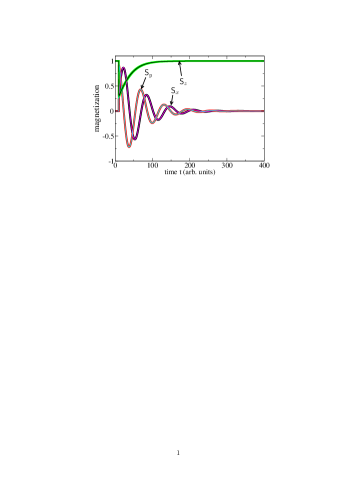
Figure 1: (color online) Magnetization as function of time after a gaussian field pulse: comparison of classical (bold lines) and quantum mechanical trajectories (thin lines).
($D_{z}=0$, $\mu_{S}B_{z}=0.1$, $T_{W}=0.02$, $t_{0}=10$, $\mu_{S}B_{0}^{x}=25.27$, and $\lambda=0.2$)

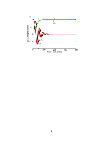
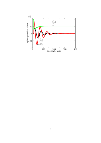
Figure 2: (color online) Magnetization as function of time after a gaussian field pulse: (a) classical trajectory $S_{\eta}$, (b) quantum mechanical expectation values $\langle\hat{S}_{\eta}\rangle$, $\eta\in\{x,y,z\}$
($D_{z}=0.1$, $\mu_{S}B_{z}=0$, $T_{W}=0.02$, $t_{0}=10$, $\mu_{S}B_{0}^{x}=25.27$, and $\lambda=0.2$)

To prove the agreement between the TDSE and the Landau-Lifshitz Eq. we have performed numerical calculations. In the following we use a simple single spin model. The description is just an example and can be extended to systems with $N>1$. The corresponding Hamilton operator $\hat{\mathrm{H}}$ is given by:

$$\hat{\mathrm{H}}=-D_{z}\left(\hat{S}_{z}\right)^{2}-\mu_{S}B_{z}\hat{S}_{z}-\mu_{S}B_{x}(t)\hat{S}_{x}$$ (27)

The first term of the Hamiltonian describes a uniaxial anisotropy with the $z$-axis as the easy axis. The second term represents a static external magnetic field in $+z$-direction. The last term is a time-dependent field pulse

$$B_{x}(t)=B_{0}^{x}{\mathrm{e}}^{-\frac{1}{2}\left(\frac{t-t_{0}}{T_{W}}\right)^{2}}$$ (28)

with gaussian shape to excite the spin. In an experimental setup using single atoms such an excitation can be realized, e.g., by a current pulse coming from an STM (scanning tunneling microscope) tip. In the following we investigate the two situations: either (i) $D_{z}=0$ and $B_{z}\neq 0$ or vice versa (ii) $D_{z}\neq 0$ and $B_{z}=0$. In the case (i) all terms of the Hamiltonian are linear in $\hat{\mathbf{S}}$. In the second case (ii) the Hamiltonian contains a quadratic term.

In a previous publication Wieser (2011) we have shown that in case (i) under the assumption of a negligible damping $(\lambda=0)$ a good agreement between classical and quantum spin dynamics can be obtained. Case (ii) shows without relaxation a disagreement between classical and quantum spin dynamics due to the noncommutativity of the quadratic terms.

Fig. 1 shows the results of the calculation of a single spin with relaxation for the case (i) (without anisotropy). Again an excellent agreement between quantum mechanical expectation values $\langle\hat{S}_{\eta}\rangle$ $\eta\in\{x,y,z\}$ and the classical trajectories $S_{\eta}$ of Landau-Lifshitz Eq. is found. In case (ii) [Fig. 2] the classical trajectories (a) and quantum mechanical expectation values (b) disagree. This is caused by the quadratic Hamilton operator due to the anisotropy Wieser (2011). In this case the commutator $[\mathbf{\hat{S}}_{n};\hat{\mathrm{H}}]$ leads to $\mathbf{\hat{S}}\times\partial\hat{\mathrm{H}}/\partial{\mathbf{S}}$ plus an additional term of the order of $\hbar$. This additional term vanishes in the classical limit $S\rightarrow\infty$ and leads to the disagreement between quantum mechanical and classical trajectory. In the case of a linear Hamiltonian the commutator $[\mathbf{\hat{S}}_{n};\hat{\mathrm{H}}]$ does not lead to an additional correction and the both trajectories show a perfect agreement. Therefore, we can say that the second commutator in the damping term does not produce any corrections.

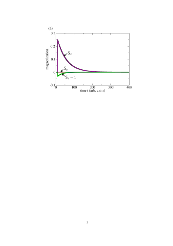
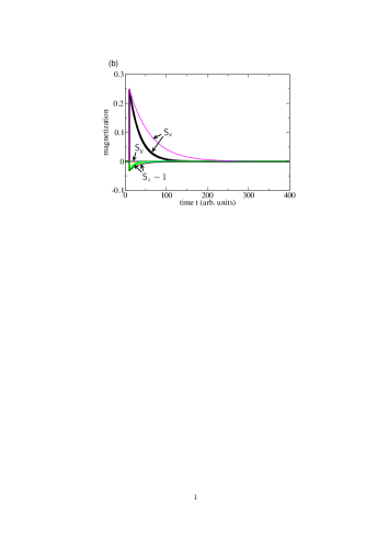
Figure 3: (color online) Overdamped relaxation of magnetization after a gaussian field pulse. ${\sf S}_{\alpha}$, $\alpha\in\{x,y,z\}$ corresponds to classical (bold lines) resp. to quantum mechanical trajectories (thin lines). (a) $D_{z}=0$ and $\mu_{S}B_{z}=0.1$, (b) $D_{z}=0.1$ and $\mu_{S}B_{z}=0$. ($T_{W}=0.02$, $t_{0}=10$, $\mu_{S}B_{0}^{x}=25.27$, and $\lambda=0.2$)

In the case of the quadratic Hamiltonain with anisotropy we have the additional term Wieser (2011) $\mathrm{i}D_{z}/\hbar\,(\hat{S}_{n}^{x},\hat{S}_{n}^{y},0)$ which commutes with $\mathbf{\hat{S}}$. Therefore the deviation between classical and quantum trajectory does not come from this term. The question is whether this correction comes from the precessional term $-\mathrm{i}/\hbar[\mathbf{\hat{S}}_{n};\hat{\mathrm{H}}]$ only or whether the relaxation term $\lambda/\hbar[\mathbf{\hat{S}};[\mathbf{\hat{S}};\hat{\mathrm{H}}]]$ also leads to a correction. To answer this question and to clarify the effect of the damping we compare the trajectories in the overdamped limit $(\lambda\gg 1)$. Here we assume that the damping dominates the dynamics and skip the precessional terms: the overdamped TDSE is given by:

$$\left(\frac{\mathrm{d}}{\mathrm{d}t}+\frac{\lambda}{\hbar}[\hat{\mathrm{H}}-\langle\hat{\mathrm{H}}\rangle]\right)|\psi(t)\rangle=0\;,$$ (29)

and the overdamped Landau-Lifshitz equation by:

$$\frac{\partial{\mathbf{S}}}{\partial t}=\frac{\lambda}{\mu_{S}}{\mathbf{S}}\times\left({\mathbf{S}}\times{\mathbf{H}}_{\mathrm{eff}}\right)\,.$$ (30)

Fig. 3 shows the trajectories of the overdamped relaxation process after a field pulse excitation. As expected in case (i) $D_{z}=0$, $B_{z}\neq 0$ we see a perfect agreement between the quantum mechanical and the classical curve. In case (ii) $D_{z}\neq 0$, $B_{z}=0$ we find the deviation which means that the second commutator also produces a correction which modifies the correction which comes from the precession term.

In summary I have shown that it is possible to derive the Landau-Lifshitz equation from the quantum mechanical time evolution of a wave function. This derivation reveals the underlying mathematics and assumptions. During the derivation we get different presentations in different physical pictures and descriptions.

In quantum mechanics we can find behavior which cannot be described by classical physics like quantum tunneling. In a previous publication Wieser (2011) I have shown that quadratic or higher order Hamilton operators do not behave classical, meaning the Ehrenfest theorem does not hold in these cases. In this publication this concept has been used to proof the damping term. In the case of a linear Hamiltonian we see a perfect agreement of classical physics and quantum mechanics, but for quadratic and higher order Hamiltonians a deviation appears, which comes from the damping term. Therefore, the described formalism gives us the possibility to compare the classical with the quantum spin dynamics.

The author wants to thank N. Mikuszeit and S. Krause for helpful discussions. This work has been supported by the Deutsche Forschungsgemeinschaft (SFB 668 B3) and the Hamburg Cluster of Excellence NANOSPINTRONICS.

References

• Landau and Lifshitz (1935) D. L. Landau and E. M. Lifshitz, Phys. Z. Sowjetunion 8, 153 (1935).
• Brown (1963) W. F. Brown, Micromagnetics (Wiley, New York, 1963).
• Antropov et al. (1995) V. P. Antropov et al., Phys. Rev. Lett. 75, 729 (1995).
• Börner et al. (1975) G. Börner et al., Astron. & Astrophys. 44, 417 (1975).
• Bell et al. (2007) J. B. Bell et al., Phys. Rev. E 76, 016708 (2007).
• Hucht et al. (2007) A. Hucht et al., Europhys. Lett. 77, 57003 (2007).
• Witte et al. (2012) K. Witte et al., J. Spintr. Magn. Nanomater. 1, 40 (2012).
• F. Bloch (1946) F. Bloch, Phys. Rev. 70, 460 (1946).
• Ishimori (1984) Y. Ishimori, Prog. Theor. Phys. 72, 33 (1984).
• D. A. Garanin (1997) D. A. Garanin, Phys. Rev. B 55, 3050 (1997).
• Wieser (2011) R. Wieser, Phys. Rev. B 84, 054411 (2011).
• Gilbert (2004) T. L. Gilbert, IEEE Trans. Mag. 40, 3443 (2004).
• Mølmer et al. (1993) K. Mølmer et al., J. Opt. Soc. Am. B 10, 524 (1993).
• Gisin (1981) N. Gisin, Helv. Phys. Acta 54, 457 (1981).
• Garanin (2011) D. A. Garanin, Adv. Chem. Phys. 147, 213 (2011).
• Fano (1957) U. Fano, Rev. Mod. Phys 29, 74 (1957).
• Lakshmanan (2011) M. Lakshmanan, Phil. Trans. R. Soc. A 369, 1280 (2011).
• Liu et al. (2009) C.-S. Liu, K.-C. Chen, and C.-S. Yeh, J. of Marine Sci. and Tech. 17, 228 (2009).