Joint estimation of multiple related biological networks

Abstract

Graphical models are widely used to make inferences concerning interplay in multivariate systems. In many applications, data are collected from multiple related but nonidentical units whose underlying networks may differ but are likely to share features. Here we present a hierarchical Bayesian formulation for joint estimation of multiple networks in this nonidentically distributed setting. The approach is general: given a suitable class of graphical models, it uses an exchangeability assumption on networks to provide a corresponding joint formulation. Motivated by emerging experimental designs in molecular biology, we focus on time-course data with interventions, using dynamic Bayesian networks as the graphical models. We introduce a computationally efficient, deterministic algorithm for exact joint inference in this setting. We provide an upper bound on the gains that joint estimation offers relative to separate estimation for each network and empirical results that support and extend the theory, including an extensive simulation study and an application to proteomic data from human cancer cell lines. Finally, we describe approximations that are still more computationally efficient than the exact algorithm and that also demonstrate good empirical performance.

FLA

, , and

T1Supported in part by NCI U54 CA112970, UK EPSRC EP/E501311/1 and EP/D002060/1, and the Cancer Systems Biology Center grant from the Netherlands Organisation for Scientific Research. T2A recipient of a Royal Society Wolfson Research Merit Award.

1 Introduction

Graphical models are widely used to represent multivariate systems. Vertices in a graph (or network; we use both terms interchangeably) $G$ are identified with random variables and edges between the vertices describe conditional independence statements or, with suitable modeling and semantic extensions, causal influences between the variables. In many applications a key statistical challenge is to construct a network estimator $\hat{G}(\mathbf{y})$, based on data $\mathbf{y}$, that performs well in a sense appropriate to the application. Such “network inference” is increasingly a mainstream approach in many disciplines, including neuroscience, sociology and computational biology.

Network inference methods usually assume that the data are identically distributed (specifically, that data sets satisfy an exchangeability assumption). However, in many applications, data are not identically distributed, but are instead obtained from multiple related but nonidentical units (or “individuals”; we use both terms interchangeably). This paper concerns network inference in this nonidentically distributed setting.

Our work is motivated by biological networks in cancer. Multiple studies have demonstrated the remarkable genomic heterogeneity of cancer [The 1000 Genomes Project Consortium (2010), The Cancer Genome Atlas Network (2012)]. At the same time, the question of how such heterogeneity is manifested at the level of biological networks has remained poorly understood. We focus in particular on protein signaling networks in human cancer cell lines. Signaling networks describe biochemical interplay between proteins and are central to cancer biology. However, sequence and transcript data alone are inadequate for the study of signaling and, indeed, these data types can be discordant with the abundance of signaling proteins and post-transitional modifications (including phosphorylation) that are key to the process [Akbani et al. (2014)]. Recent developments in proteomics, including reverse-phase protein arrays [or RPPA, see Hennessy et al. (2010); this technology provides the data we analyze below], have improved the ability to interrogate signaling heterogeneity.

To fix ideas, we begin by describing the specific application that motivates this work. We consider time-course phosphoprotein measurements obtained using RPPA technology (details appear below) for 6 cell lines. The goal of the study is to infer cell line-specific protein signaling networks $G^{j}$, $j=1,\ldots,6$, and additionally to highlight experimentally testable differences between them. Prior network information is available from the literature, but it is believed that cell line-specific genetic alterations may induce differences with respect to the “literature network” (and between cell lines). At the same time, the amount of data per cell line is limited (6 time points in each of 4 conditions, making a total of 24 data points per cell line $j$, constituting data $\mathbf{y}^{j}$). Since the cell lines $j$ are closely related, yet potentially different with respect to underlying networks, a key inferential question is how to “borrow strength” between the network estimation problems. That is, we seek a joint estimator of the cell line-specific networks $\{G^{1}\cdots G^{6}\}$ based on the entire (nonidentically distributed) data set $\{\mathbf{y}^{1}\cdots\mathbf{y}^{6}\}$ that shares information between the estimation problems while preserving the ability to identify cell line-specific network structure.

This application is an example of a more general class of biological applications, where individuals $j$ could correspond to, for example, different patients or cell lines (or groups thereof; e.g., disease subtypes) and the networks themselves to gene regulatory or protein signaling networks that could depend on the genetic and epigenetic state of the individuals. Indeed, continuing reduction in the unit cost of biochemical assays has led to an increase in experimental designs that include panels of potentially heterogeneous individuals [Barretina et al. (2012), Cao et al. (2011), Maher (2012), The Cancer Genome Atlas Network (2012)]. As in the signaling example above, in such settings, given individual-specific data $\mathbf{y}^{j}$, there is scientific interest in individual-specific networks $G^{j}$ and their similarities and differences.

Following Werhli and Husmeier (2008), Penfold et al. (2012) and others, we focus on the case of directed networks $G^{j}$ that are exchangeable in the sense that inference is invariant to permutation of individuals $j\in\mathcal{J}=\{1,\ldots,J\}$. We model data on all individuals $\{\mathbf{y}^{j}\dvtx j\in\mathcal{J}\}$ within a joint Bayesian framework. Regularization of individual networks is achieved by introducing a latent network $G$ to couple inference across all individuals. We report posterior marginal inclusion probabilities for every possible edge in each individual network $G^{j}$ as well as the latent network $G$. The high-level formulation we propose is general and, in principle, essentially any graphical model of interest could be embedded within the framework described to enable joint estimation.

In general, the individual $j$’s could have complex, hierarchical relationships, for example, with $j$’s belonging to groups and subgroups [e.g., corresponding to cancer types and subtypes; see Curtis et al. (2012)]. The exchangeable case we consider corresponds in a sense to the simplest possible hierarchy in which each individual is dependent on a single latent graph (see Figure 1). In settings where groups can be treated as approximately homogeneous, the approach presented in this paper can be trivially used to give group-level estimates, by using $j$ to index groups rather than individuals, with all data for group $j$ modeled as dependent on graph $G^{j}$. This corresponds to an assumption of identically distributed data within (but not between) groups. In the empirical study presented below we consider also robustness of our approach under violation of the exchangeability assumption.

For the application to time-course data from protein signaling that we focus on, we present a detailed development using directed graphical models called dynamic Bayesian networks (DBNs). These are directed acyclic graphs (DAGs) with explicit time indices [Murphy (2002)]. The main contributions of this paper are as follows:

• Bayesian computation. For the time-course setting, we put forward an efficient and exact algorithm. This is done by exploiting factorization properties of the DBN likelihood, analytic marginalization over continuous parameters and belief propagation. In moderate dimensional settings this allows exact joint estimation to be carried out in seconds to minutes (we discuss computational complexity below).

• Theory. We provide a result that quantifies the statistical efficiency of joint relative to separate estimation and that gives a sufficient condition for improved performance.

• Empirical investigation. The availability of an efficient Bayesian algorithm enables, for the first time, a comprehensive empirical study of joint estimation, including a wide range of simulation regimes and an application to experimental data from a panel of human cancer cell lines. For several classical (nonjoint) DBNs, including a recent causal variant suitable for interventional data [Spencer, Hill and Mukherjee (2012)], we formulate corresponding joint estimators. This allows us to investigate the effect of joint estimation itself; we find that it often provides gains relative to the corresponding individual-level estimators. Some computationally favorable approximations to joint inference are described that we find perform well under a range of conditions.

Joint estimation has previously been discussed in the Gaussian graphical model (GGM) literature [Danaher, Wang and Witten (2014)]. In contrast to GGMs, motivated by biological applications, we focus on DAG models with a causal interpretation. Approaches to context-specific DAG structure based on the embellishment of Bayesian networks include Boutilier et al. (1996), Geiger and Heckerman (1996). Our approach differs by regularizing based on network structure alone; we do not place exchangeability assumptions on the data-generating parameters. Related work that is based on DAGs includes Niculescu-Mizil and Caruana (2007), Werhli and Husmeier (2008), Dondelinger, Lèbre and Husmeier (2013). In a sequel to the present work, Oates, Costa and Nichols (2014) provide an exact algorithm for joint maximum a posteriori (MAP) estimate of multiple (static) DAGs. In contrast, here we focus on Bayesian model-averaging (as opposed to MAP estimation) and on time-course data (or, more generally, Bayesian networks with a fixed ordering of the variables).

In a similar vein to the present paper, Oyen and Lane (2013) estimated multiple DAGs sharing a common ordering of the vertices, but they considered only applications involving $J=2$ individuals. Our work is closely related to Penfold et al. (2012), who also considered Bayesian joint estimation of directed graphs from time-course data. However, as we discuss in detail below, the methodology they propose is prohibitively computationally expensive for the applications we consider here. In comparison, the exact algorithm we propose offers massive computational gains that in turn allow us to present a much more extensive study of joint estimation than has hitherto been possible. Furthermore, we allow for prior information regarding the network structure (including individual-specific characteristics) and present theoretical results concerning the statistical efficiency of joint network estimation.

The remainder of the paper is organized as follows. In Section 2 we describe a hierarchical Bayesian formulation and in Section 3 we discuss computationally efficient joint inference in the case of DBNs. Empirical results are presented in Section 4, including an application to protein signaling in cancer. Finally, we close with a discussion of our findings in Section 5.

2 Joint network inference: The general case

We describe a general statistical formulation for joint network inference that can be coupled to essentially any class of graphical models. For computational tractability it may be necessary to place restrictions on the class of graphical models; in Section 3 we present a detailed development for DBNs that are well-suited to our motivating application in cancer.

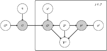
Figure 1: Joint network inference (JNI). A hierarchical model for analysis of multivariate data from multiple, nonidentical units or individuals, indexed by $j$. (Shaded nodes are unobserved. $G^{0}={}$prior network, $G={}$latent network, $G^{j}={}$network specific to individual $j$, $\bolds{\theta}^{j}={}$parameters for individual $j$, $\mathbf{Y}^{j}={}$observables for individual $j$, $Z^{j}={}$ancillary information available on individual $j$, $\eta,\lambda^{j}={}$inverse temperature hyperparameters, $\phi^{j}={}$hyperparameters defining a prior on $\bolds{\theta}^{j}$. Panel notation is used to indicate the presence of multiple individuals $j\in\mathcal{J}$. Note that in practice we take $\lambda_{j}\equiv\lambda$ for all $j\in\mathcal{J}$.)

2.1 Hierarchical model

Consider a space $\mathcal{G}$ of graphs on the vertex set $\mathcal{P}=\{1,\ldots,P\}$. To keep the presentation general, we do not specify the type of graph or restrictions on $\mathcal{G}$ at this stage (the special case of DBNs for time-course data is described below). As shown in Figure 1, each individual network $G^{j}\in\mathcal{G}$ is modeled with dependence on a latent network $G\in\mathcal{G}$ that in turn depends on a prior network $G^{0}\in\mathcal{G}$ (Section 2.2). In this way, estimates of the individual networks $G^{j}$ are regularized by shrinkage toward the common latent network $G$ that, in turn, may be constrained by an informative network prior. As in any graphical model, observations $\mathbf{Y}^{j}$ on individual $j$ are dependent upon a graph $G^{j}$ and parameters $\bolds{\theta}^{j}$. Here $Z^{j}$ denotes any ancillary information available on individual $j$. The model is specified by

$$p\bigl{(}G|G^{0},\eta\bigr{)} \propto \exp\bigl{(}-\eta d\bigl{(}G,G^{0}\bigr{)}\bigr{)},$$ (1)

$$p\bigl{(}G^{j}|G,\bolds{\lambda},Z^{j}\bigr{)} \propto \exp\bigl{(}-\lambda^{j}d^{j}\bigl{(}G^{j},G;Z^{j}\bigr{)}\bigr{)}$$ (2)

and a suitably chosen graphical model likelihood $p(\mathbf{Y}^{j}|G^{j},\bolds{\theta}^{j},Z^{j})$. Equation (1) follows the “network prior” approach of Mukherjee and Speed (2008) that was proposed for biological applications where subjective prior structural information is available. The functionals $d^{j},d\dvtx\mathcal{G}\times\mathcal{G}\rightarrow\mathbb{R}$ and hyperparameters $\eta,\lambda^{j}$ must be specified (Section 2.2). This paper restricts attention to exchangeable models, in particular, we consider functionals $d^{j}$ that are independent of the index $j$. We refer to the above formulation as joint network inference (JNI).

2.2 Network prior

The network prior [equation (1)] requires a penalty functional $d\dvtx\mathcal{G}\times\mathcal{G}\rightarrow\mathbb{R}$ and a prior network $G^{0}\in\mathcal{G}$, with the former capturing how close a candidate network $G\in\mathcal{G}$ is to the latter. We discuss choice of $G^{0}$ below. Given $G^{0}$, a simple choice of penalty function $d$ is the structural Hamming distance (SHD) given by $d(G,G^{0})=\|G-G^{0}\|$, where $\|M\|=\sum_{i,j}|m_{i,j}|$ is the $\ell_{1}$-norm of an adjacency matrix and the differential network $G-G^{0}$ is defined to have edges that occur in exactly one of the networks $G$, $G^{0}$ [see also Ibrahim and Chen (2000), Imoto et al. (2003)]. The hyperparameter $\eta$ controls the strength of the prior network $G^{0}$ [equation (1)]. Motivated by an application in cancer biology where prior structural information $G^{0}$ is available, we follow Penfold et al. (2012) by restricting attention to SHD priors, however, our statistical formulation is general (see below) and compatible with other penalty functionals. Alternatively, one could employ a beta-binomial prior as described in, for example, Dondelinger, Lèbre and Husmeier (2013), that allows for the hyperparameters of the binomial to be integrated out [see also Oyen and Lane (2013)]. Note that in the latter case it is not possible to integrate specific prior structural information, making beta-binomial priors unsuitable for the application that this paper considers.

Given a latent network $G$, individual networks $G^{j}$ are regularized in a similar way, as $d^{j}(G^{j},G)=\|G^{j}-G\|$. In their work on combining multiple data sources, Werhli and Husmeier (2008) allow the $\lambda^{j}$ to vary over individuals $j\in\mathcal{J}$. Likewise, Penfold et al. (2012) learn the $\lambda^{j}$ on a per-individual basis. However, in both studies, hyperparameter elicitation is nontrivial (see Section 3.3). In the present paper, we consider only the special case where $\lambda^{1}=\lambda^{2}=\cdots=\lambda^{J}:=\lambda$.

A graph $G\in\mathcal{G}$ can be characterized by (i) its adjacency matrix or (ii) its parent sets as $G=(\pi_{1},\ldots,\pi_{P})$, where $\pi_{p}\subseteq\mathcal{P}=\{1\cdots P\}$ are the parents of vertex $p$ in $G$. We write $\mathcal{G}_{p}$ for the set of possible parent sets for $p$, such that formally $\mathcal{G}=\mathcal{G}_{1}\times\cdots\times\mathcal{G}_{P}$. Although we focus on SHD priors, the inference procedures presented in this paper apply to the more general class of “modular” priors, that may be factored over $p\in\mathcal{P}$ and written in the form

$$d\bigl{(}G,G^{0}\bigr{)}=\sum_{p\in\mathcal{P}}d_{p}\bigl{(}\pi_{p},\pi_{p}^{0}\bigr{)},d^{j}\bigl{(}G^{j},G;Z^{j}\bigr{)}=\sum_{p\in\mathcal{P}}d_{p}^{j}\bigl{(}\pi_{p}^{j},\pi_{p};Z^{j}\bigr{)}$$ (3)

for some functionals $d_{p},d_{p}^{j}\dvtx\mathcal{G}_{p}\times\mathcal{G}_{p}\rightarrow\mathbb{R}$. Here $\pi_{p}^{0}$ and $\pi_{p}^{j}$ are parent sets for variable $p$, corresponding to $G^{0}$ and $G^{j}$, respectively.

In general, inference for the JNI model [equations (1), (2)] will be computationally intensive, as demonstrated in Werhli and Husmeier (2008), Penfold et al. (2012). In Section 3 below we show that efficient, exact inference is nevertheless possible within the DBN class of graphical models.

3 Joint network inference: DBNs

The JNI model and network priors, as described above, are general. To apply the JNI framework in a particular context requires an appropriate likelihood at the individual level, that is, specification of the joint distribution $p(\mathbf{Y}^{j}|G^{j},\bolds{\theta}^{j},Z^{j})$ of observables $\mathbf{Y}^{j}$ given network $G^{j}$, ancillary information $Z^{j}$ and parameters $\bolds{\theta}^{j}$, together with a prior distribution $p(\bolds{\theta}^{j}|G^{j},Z^{j})$ over model parameters. We focus on time-course data, using DBNs and exploiting families of conjugate prior distributions. We show that factorization properties of the DBN likelihood permit computationally tractable joint inference and provide an explicit algorithm based on belief propagation.

3.1 DBN formulation

A DBN is a graphical model based on a DAG on the vertex set $\mathcal{P}\times\mathcal{T}$, where $\mathcal{T}$ is a set of time indices [Figure 8(a); see Murphy (2002)]. This DAG with $PT$ vertices is known as the “unrolled” DAG. Here, following Hill et al. (2012) and others, we use DBNs that permit only edges forward in time and that are stationary in the sense that neither the network nor parameters change with time. For such DBNs, the network can be described by a directed graph $G$ with exactly $P$ vertices, with edges understood to go forward in time in the unrolled DAG [see Appendix B and Figure 8(b)]. Note that $G$ may have cycles. In what follows, all graphs (prior, latent and individual) describe the latter $P$-vertex representation.

Under a modular network prior, structural inference for DBNs can be carried out efficiently as described in Hill et al. (2012). In brief, the posterior $G^{j}|\mathbf{y}$ factorizes into a product of local posteriors $\pi_{p}^{j}|\mathbf{y}$, one factor for each target variable $p$. Background and assumptions for DBNs are summarized in Appendix B; for general background on DBNs we refer the interested reader to Murphy (2002) and for relevant details concerning the class of DBNs used here to Hill et al. (2012).

Write $\mathbf{y}(t)$ for the matrix of observed data at time $t$ for all individuals $j$ and variables $p$. In order to simplify notation, we define a data-dependent functional

$$\mathfrak{P}(\mathbf{X})=p\bigl{(}\mathbf{X}(1)\bigr{)}\prod_{t=2}^{m}p\bigl{(}\mathbf{X}(t)|\mathbf{y}(t-1)\bigr{)}$$ (4)

that implicitly conditions upon observed history. Let $y_{p}^{j}(t)$ denote the observed value of variable $p$ in individual $j$ at time $t$. The above notation allows us to conveniently summarize the product

$$p\bigl{(}y_{p}^{j}(1)|\pi_{p}^{j}\bigr{)}p\bigl{(}y_{p}^{j}(2)|\mathbf{y}(1),\pi_{p}^{j}\bigr{)}\cdots p\bigl{(}y_{p}^{j}(m)|\mathbf{y}(m-1),\pi_{p}^{j}\bigr{)}$$ (5)

as $\mathfrak{P}(\mathbf{y}_{p}^{j}|\pi_{p}^{j})$. Thus, we have that, for DBNs, the full likelihood also satisfies

$$p\bigl{(}\mathbf{y}|G^{1},\ldots,G^{J},Z^{1},\ldots,Z^{J}\bigr{)}=\prod_{j\in\mathcal{J}}\prod_{p\in\mathcal{P}}\mathfrak{P}\bigl{(}\mathbf{y}_{p}^{j}|\pi_{p}^{j},Z^{j}\bigr{)},$$ (6)

where $\mathbf{y}$ denotes the complete data (for all individuals, variables and times). In other words, the parent sets $\pi_{p}^{j}$ for $p\in\mathcal{P}$, $j\in\mathcal{J}$ are mutually orthogonal in the Fisher sense, so that inference for each may be performed separately.

3.2 Efficient, exact joint estimation

We carry out exact inference in this setting using belief propagation [Pearl (1982)]. Belief propagation is an iterative procedure in which messages are passed between variables in such a way as to compute exact marginal distributions; in this respect belief propagation belongs to a more general class of iterative algorithms known as “sum-product” algorithms [Kschischang, Frey and Loeliger (2001)]. Our algorithm is summarized as follows (for simplicity we suppress dependence upon ancillary information $Z^{j}$):

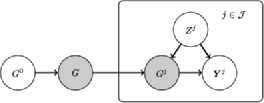
Figure 2: Marginalization of JNI over continuous (unknown) parameters $\bolds{\theta}^{j}$. (Shaded nodes are unobserved. $G^{0}={}$prior network, $G={}$latent network, $G^{j}={}$network specific to individual $j$, $\mathbf{Y}^{j}={}$observables for individual $j$, $Z^{j}={}$ancillary information available on individual $j$. Hyperparameters $\eta$, $\lambda^{j}$, $\phi^{j}$ are suppressed for clarity. Panel notation is used to indicate the presence of multiple individuals $j\in\mathcal{J}$.)

[(3)]

We begin by marginalizing over parameters $\bolds{\theta}^{j}$ and caching the local scores $\mathfrak{P}(\mathbf{y}_{p}^{j}|\pi_{p}^{j})$ for all parent sets $\pi_{p}^{j}\in\mathcal{G}_{p}$, all variables $p\in\mathcal{P}$ and all individuals $j\in\mathcal{J}$; these could be obtained using any DBN likelihood. In this paper we exploited conjugate priors to obtain exact expressions for marginal likelihoods [equation (C), see Appendix C for details].

Following marginalization, the JNI graphical model collapses to the discrete Bayesian network shown in Figure 2, whose nodes are themselves graphs.

Posterior marginal distributions $p(\pi_{p}|\mathbf{y}_{p},\pi_{p}^{0})$ and $p(\pi_{p}^{j}|\mathbf{y}_{p},\pi_{p}^{0})$ are then computed using belief propagation on this discrete Bayesian network. Pseudocode for this step is provided in Algorithm 1 in Appendix D.

Let $\mathbf{A}_{\mathrm{JNI}}$ denote the $P\times P$ matrix of marginal posterior inclusion probabilities for edges in the latent network $G$, that is, $(\mathbf{A}_{\mathrm{JNI}})_{ip}:=p(i\in\pi_{p}|\mathbf{y},G^{0})$. These quantities are analogous to posterior inclusion probabilities in Bayesian variable selection and are computed, using Bayesian model averaging, as

$$(\mathbf{A}_{\mathrm{JNI}})_{ip}=p\bigl{(}i\in\pi_{p}|\mathbf{y},G^{0}\bigr{)}=\sum_{\pi_{p}\in\mathcal{G}_{p}}\mathbf{1}_{i\in\pi_{p}}p\bigl{(}\pi_{p}|\mathbf{y},\pi_{p}^{0}\bigr{)},$$ (7)

where $\mathbf{1}_{A}$ is the indicator of the event $A$ and similarly for individual networks $(\mathbf{A}_{\mathrm{JNI}}^{j})_{ip}:=p(i\in\pi_{p}^{j}|\mathbf{y},G^{0})$.

Following Hill et al. (2012), we reduced the space of parent sets $\mathcal{G}_{p}$ using an in-degree sparsity restriction of the form $|\pi_{p}^{j}|\leq c$ for all $\pi_{p}^{j}\in\mathcal{G}_{p}$, $p\in\mathcal{P}$, $j\in\mathcal{J}$. Thus, the cardinality of the space of parent sets $|\mathcal{G}_{p}|=\mathcal{O}(P^{c})$ is polynomial in $P$, where it was previously super-exponential. As in variable selection, the bound $c$ should be chosen large enough that $\mathcal{G}_{p}$ includes the true data-generating model with high probability.

Caching of selected probabilities is used to avoid redundant recalculation. Pseudocode is provided in Algorithm 1 in Appendix D, consisting of three phases of computation. Storage costs are dominated by phases I and II, each requiring the caching of $\mathcal{O}(JP^{1+c})$ terms. Phase II dominates computational effort, with total (serial) algorithmic complexity $\mathcal{O}(J^{2}P^{1+2c})$. However, within-phase computation is “embarrassingly parallel” in the sense that all calculations are independent (indicated by square parentheses notation in the pseudocode). In practice, we have found that problems of size $P\leq 20$, $J\leq 20$, $c\leq 3$ can be solved within minutes using serial computation on a standard laptop computer. We provide serial and parallel MATLAB R2014a implementations in Supplement B [Oates et al. (2014b)].

3.3 Network prior elicitation

Elicitation of hyperparameters for network priors is an important and nontrivial issue. Here we specify the hyperparameters $\lambda,\eta$ in a subjective manner. We do so due to reported difficulties in estimation of hyperparameters for related models [Werhli and Husmeier (2008), Dondelinger, Lèbre and Husmeier (2013), Penfold et al. (2012)]. We present three criteria below that, for the special case of SHD, are simple to implement and can be used for expert elicitation. These heuristics seek to relate the hyperparameters to more directly interpretable measures of the similarity and difference that they induce between prior, latent and individual networks: (i) First, we note the following formula for the probability of maintaining the status (present/absent) of a candidate parent $i\in\mathcal{P}$ between the latent network $G$ and an individual network $G^{j}$:

$$h_{\lambda}:=p\bigl{(}i\notin\pi_{p}^{j}\Delta\pi_{p}\bigr{)}=\frac{1}{1+e^{-\lambda}}.$$ (8)

This probability provides an interpretable way to consider the influence of $\lambda$. For example, a prior confidence of $h_{\lambda}\approx 0.73$ that a given edge status in $G$ is preserved in a particular individual $G^{j}$ translates into an odds ratio $h_{\lambda}/(1-h_{\lambda})\approx 2.7$ and a hyperparameter $\lambda\approx 1$ (see SFigure 1 in the supplementary material [Oates et al. (2014a)]). An analogous equation relates $\eta$ and $h_{\eta}:=p(i\notin\pi_{p}\Delta\pi_{p}^{0})$, allowing prior strength to be set in terms of the probability that an edge status in the prior network $G^{0}$ is maintained in the latent network $G$. (ii) A second, related approach is to consider the expected total SHD between an individual network $G^{j}$ and the latent network $G$:

$$\mathbb{E}\bigl{(}\bigl{\|}G^{j}-G\bigr{\|}\bigr{)}=P^{2}(1-h_{\lambda}).$$ (9)

This can be interpreted as the average number of edge changes needed to obtain $G^{j}$ from $G$. An analogous equation holds for $\eta$ and $h_{\eta}$. (iii) Third, in certain applications, the latent network $G$ may not have a direct scientific interpretation, in which case the criteria presented above may be unintuitive. Then, hyperparameters can be elicited by consideration of (a) similarity between individual networks $G^{j},G^{k}$ and (b) concordance of individual networks $G^{j}$ with the prior network $G^{0}$ (see Supplement A [Oates et al. (2014a)] for further discussion).

3.4 An information sharing bound

Below we consider the extent to which information can be shared between individuals within JNI, providing an upper bound that is attained as the number of individuals $J$ grows large. To formalize the contribution to inference from information sharing, we consider the case in which no data is available on a specific individual (without loss of generality, individual $j=1$) and analytically quantify the extent to which JNI can estimate the true network $\overline{G^{1}}$ by “borrowing strength” from the data $\mathbf{Y}^{2},\ldots,\mathbf{Y}^{J}$ that represent observations on the remaining individuals. (Over-lines will be used to signify the “true” data-generating networks.) As a baseline, write $\mathbf{A}_{0}^{j}=p(i\in\pi_{p}^{j}|\mathbf{Y}^{j})$ for the (naive) estimator that prohibits the sharing of information between individuals. For simplicity we restrict attention to the case where no network prior is used ($\eta=0$), the data-generating hyperparameter $\lambda$ is known and in-degree restrictions are not in place ($c=P$). Then, with neither data nor prior information available on individual $1$, it trivially follows that

$$\mathbb{E}_{\mathbf{Y},\overline{G},\overline{G^{1}},\ldots,\overline{G^{J}}|\eta,\lambda}\biggl{[}\frac{\|\mathbf{A}_{0}^{1}-\overline{G^{1}}\|}{P^{2}}\biggr{]}=\frac{1}{2},$$ (10)

where the expectation is taken over all possible data-generating networks and corresponding data.

From standard, independent network inference we know that consistent estimation requires unbiasedness of the likelihood function $p(\mathbf{Y}^{j}|G^{j})$, in the sense that $\mathbb{E}_{\mathbf{Y}^{j}|\overline{G^{j}}}p(\mathbf{Y}^{j}|G^{j})$ is maximized by $G^{j}=\overline{G^{j}}$. We therefore begin by constructing the analogous regularity condition for joint estimation: Write $\mathbf{R}$ for the matrix that encodes the prior metric on $\mathcal{G}$ as $(\mathbf{R})_{G,G^{\prime}}=\exp(-\lambda\|G-G^{\prime}\|)/C(\lambda)$, where $C(\lambda)=\sum_{G\in\mathcal{G}}\exp(-\lambda\|G\|)$. Write $\mathbf{S}$ for the matrix of expected Bayesian scores $(\mathbf{S})_{G^{j},\overline{G^{j}}}=\mathbb{E}_{\mathbf{Y}^{j}|\overline{G^{j}}}p(\mathbf{Y}^{j}|G^{j})$.

[(Joint regularity)] For each column of the matrix $\mathbf{M}=(\mathbf{R}\mathbf{S}\mathbf{R})_{G,\overline{G}}$, the nondiagonal entries are strictly smaller than the diagonal entry, that is, $M_{G,\overline{G}}<M_{\overline{G},\overline{G}}$ for all $G\neq\overline{G}$.

To gain intuition for the joint regularity assumption, consider the special case where $\lambda\rightarrow\infty$; here $\mathbf{R}=\mathbf{I}$ and we only require that the expected local Bayesian score $(\mathbf{S})_{G^{j},\overline{G^{j}}}$ is maximized by $G^{j}=\overline{G}$, that is, we recover the unbiasedness condition from standard network inference.

Under the joint regularity assumption, there exists $0<\varepsilon<1$ such that

$$\mathbb{E}_{\mathbf{Y},\overline{G},\overline{G^{1}},\ldots,\overline{G^{J}}|\eta,\lambda}\biggl{[}\frac{\|\mathbf{A}_{\mathrm{JNI}}^{1}-\overline{G^{1}}\|}{P^{2}}\biggr{]}=f(J)+\frac{1}{1+e^{\lambda}},$$ (11)

where $f(J)\leq 2P^{2}\varepsilon^{J-1}\rightarrow 0$ as $J\rightarrow\infty$.

See Appendix A.

Comparing equation (11) to (10), we see that information sharing offers gains in estimation, agreeing with intuition, with larger gains when the true networks are almost homogeneous ($\lambda$ large). Moreover, the statistical power of JNI to estimate $\overline{G^{1}}$ converges to its maximum exponentially quickly as $J\rightarrow\infty$.

4 Results

The proposed methodology was compared against several existing network inference algorithms. We restricted attention to methods that are compatible with time-course data and, following the majority of the literature, carry out estimation for each individual separately. The computational demands of Niculescu-Mizil and Caruana (2007), Werhli and Husmeier (2008), Penfold et al. (2012) precluded application in this setting. Specifically, in the simulated data examples we report below, over 3000 rounds of inference were performed in total, on problems larger than DREAM4 ($P=10$, $J=5$). Using the approach of Penfold et al. (2012), these experiments would have required more than 10 years serial computational time; in contrast, our approach required less than 24 hours serial computation on a standard laptop. Thus, we consider the following methods:

[(iii)]

DBN. A dynamic Bayesian network, as described in Hill et al. (2012), including nonlinear interaction terms. For this choice of model it is possible to construct a fully conjugate set of priors, delivering a closed-form expression for the local Bayesian score $\mathfrak{P}(\mathbf{y}_{p}^{j}|\pi_{p}^{j},Z^{j})$. The model is summarized in Appendix B.

IDBN. Spencer, Hill and Mukherjee (2012) recently proposed an extension of Hill et al. (2012) that allows analysis of data sets that contain interventions; this is outlined in Appendix B. Interventional DBNs (IDBNs) inherit the computational advantages of DBNs, in the sense that there is a closed-form expression for the local Bayesian score, but extend DBNs in a causal direction. We considered two alternative implementations of IDBNs: (i) IDBN. The approach of Spencer, Hill and Mukherjee (2012) was applied to each individual separately. (ii) Mono IDBN. Data on all individuals were pooled together and fed into a single IDBN analysis, an approach that Werhli and Husmeier (2008) described as “monolithic.”

Rel Nets. A popular approach within the bioinformatics community is to score edges based on Pearson correlation of participating nodes [“relevance networks”; see, e.g., Butte et al. (2000)]. Here, we used a time-course analogue in which the correlation is calculated between successive time points.

LASSO. An $\ell_{1}$-penalized likelihood was used to obtain estimates for coefficients in a linear autoregressive model. Coefficients were estimated for each variable independently, taking each variable in turn as the response. The penalty parameters $\lambda_{p}$ were each selected using leave-one-out cross-validation. Nonzero coefficients indicated the presence of edges. Further details appear in Supplement A [Oates et al. (2014a)]. Note that DBN and IDBN are able to integrate a prior network $G^{0}$, whereas Rel Nets and LASSO are not. JNI facilitates joint estimation given a suitable graphical model likelihood. We applied JNI to the DBN and IDBN models described above. This resulted in several proposed estimators:

[(viii)]

J-DBN. JNI applied to DBN.

J-IDBN. JNI applied to IDBN.

Fixed IDBN. Here we formed the likelihood assuming a single graph for all individuals and the latent network (i.e., $G^{1}=\cdots=G^{J}=G$) but with parameters allowed to differ. This can be considered a joint analogue of Mono IDBN that allows individual-specific parameter values.

AJ-IDBN. A computationally efficient approximation to J-IDBN, in which the latent network topology is first estimated using Fixed IDBN. This is in turn used as an informative network prior within $J$ independent rounds of IDBN. In this way information sharing is allowed to occur, but at the expense of a coherent joint posterior.

In the empirical study below we compare JNI variants (v)–(viii) against existing methods (i)–(iv).

4.1 Performance metrics

The proposed methodology addresses three questions, some or all of which may be of scientific interest depending on the application: (i) estimation of the latent network $G$, (ii) estimation of individual networks $G^{1},\ldots,G^{J}$, and (iii) estimation of differences between individual networks [“differential networks”; Ideker and Krogan (2012)]. We quantify performance for each task using the area under the receiver operating characteristic (ROC) curve (AUR). This metric, equivalent to the probability that a randomly chosen true edge is preferred by the inference scheme to a randomly chosen false edge, summarizes, across a range of thresholds, the ability to select edges in the data-generating network. AUR may be computed relative to the true latent network $G$ or relative to the true individual networks $G^{j}$, quantifying performance on tasks (i) and (ii), respectively. Both sets of results are presented below, in the latter case averaging AUR over all individual networks. For (iii), in order to assess ability to estimate differential networks, we computed AUR scores based on the statistics $F_{ip}^{j}=|p(i\in\pi_{p}^{j}|\mathbf{y},G^{0},Z^{j})-p(i\in\pi_{p}|\mathbf{y},G^{0},Z^{1},\ldots,Z^{J})|$ that should be close to one if $i\in\pi_{p}^{j}\Delta\pi_{p}$, otherwise $F_{ip}^{j}$ should be close to zero.

It is easy to show that inference for the latent network, under only the prior (i.e., $\hat{G}=G^{0}$), attains mean AUR equal to $h_{\eta}$. Similarly, prior inference for the individual networks (i.e., $\hat{G}^{j}=G^{0}$) attains mean AUR equal to $1-h_{\eta}-h_{\lambda}+2h_{\eta}h_{\lambda}$. This provides a baseline for the proposed methodology at tasks (i) and (ii) and allows performance to be decomposed into AUR due to prior knowledge and AUR contributed through inference.

Using a systematic variation of data-generating parameters, we defined 15 distinct data-generating regimes described below. For all 15 regimes we considered 50 independent data sets; standard errors accompany average AUR scores. Results presented below use a computationally favorable in-degree restriction $c=3$. In order to check robustness to $c$, a subset of experiments were repeated using $c=4$, with close agreement observed (SFigure 4 in the supplementary material [Oates et al. (2014a)]).

4.2 Simulation study

4.2.1 Data generation

Data were generated according to DBN models (Appendix B) as described in detail in Supplement A [Oates et al. (2014a)]. This data-generating scheme was extended to mimic interventional experiments that are a feature of our application to breast cancer. In this case, for each time course, a randomly chosen variable is marked as the target of an interventional treatment. Data were then generated according to the augmented likelihood described in Appendix B (fixed effects were taken to be zero).

4.2.2 Model misspecification and nonlinear data-generating models

We assume exchangeable networks; it is therefore interesting to explore the performance of the proposed estimators when the assumption of exchangeability is violated. Specifically, we consider a “worst case” scenario where individual networks $G^{1},\ldots,G^{J}$ are sampled from a mixture model with two distinct components. Moreover, we consider the extreme case where networks in distinct mixture components share only a few edges in common; it is expected that exchangeable estimators will exhibit poor performance in this scenario. Further, in order to investigate the impact of model misspecification at the level of the time-series model itself, we considered time-course data generated from a computational model of protein signaling, based on nonlinear ODEs [Xu et al. (2010)]. In order to extend this model, which is for a single cell type, to simulate a heterogeneous population, we selected three protein species per individual (at random) and deleted their outgoing edges to obtain the data-generating networks $G^{j}$ (see Supplement A [Oates et al. (2014a)]).

4.2.3 Estimator performance

We consider the three estimation tasks:

Latent network

We investigated ability to recover the latent network $G$. The existing approaches (i)–(iv) estimate only individual-specific networks. For estimation of the latent, shared network using these methods, we simply took an unweighted average of the $J$ estimated adjacency matrices. The proposed joint estimators (v)–(viii) were assigned hyperparameter values $\eta=1,\lambda=2$ [$\lambda=3$ for Xu et al. (2010)] based on the heuristic of equation (8); sensitivity to misspecified hyperparameter values is investigated later in Section 4.2.4. Results based on simulated data with interventions are displayed in STable 3 (see supplementary material [Oates et al. (2014a)]). We found little difference in the ability of J-IDBN, Fixed IDBN and AJ-IDBN to recover the latent network structure across a wide range of regimes, though J-IDBN achieved best performance in 9 out of 15 regimes. Interestingly, we found that the IDBN estimator, which performs an unweighted average of $J$ independent inferences, performed significantly worse than each of J-IDBN, Fixed-IDBN and AJ-IDBN in, respectively, 15, 13 and 11 out of 15 regimes. Similarly, all the above approaches clearly outperformed Mono IDBN and Rel Nets, which were in turn outperformed by inference based on the prior alone, demonstrating the importance of accounting for individual-specific parameter values. The joint formulation of DBNs (J-DBN) significantly outperformed standard DBNs, with higher AUR in all 15 regimes. LASSO performed best in the regime with long time series ($n=10$) but failed in other regimes to outperform inference based on the prior alone. We obtained qualitatively similar results for both alternative data-generating schemes (STables 4–5, see supplementary material [Oates et al. (2014a)]).

Individual networks

At this task, J-IDBN outperformed all other approaches in 9 out of 15 regimes. AJ-IDBN offered a similar level of performance and together these estimators demonstrated better performance compared to alternatives in 13 out of 15 regimes. Since AJ-IDBN avoids intensive computation, this may provide a practical estimator of individual networks in higher dimensional settings. Again, the joint approaches J-IDBN and J-DBN both outperformed the standard approaches IDBN and DBN, respectively, demonstrating an increase in statistical power resulting from the proposed methodology. Rel Nets and LASSO performed poorly at this task. Similar results were observed using the alternative data-generating schemes (STables 4–5, see supplementary material [Oates et al. (2014a)]).

Differential networks

Since JNI regularizes between individuals, we sought to test whether it could eliminate spurious differences and thereby improve estimation of differential networks. Differential networks may also be estimated using existing methods (i)–(iv); to do so, in each case we compared individual network estimates with the estimate of the latent network obtained as described in Section 4.2.3 above. We found that, while estimation of differential networks appears to be more challenging than the other tasks, J-IDBN outperformed the other approaches in 7 out of 15 regimes. Moreover, the J-IDBN and J-DBN methods outperformed IDBN and DBN, respectively, in all 15 regimes. These results suggest that coherence of joint analysis aids in suppressing spurious features for estimation of differential network topology. Rel Nets performed poorly at this task and LASSO performed slightly better. Intriguingly, AJ-IDBN performed well in estimating differential networks, performing best in 7 out of 15 regimes. This suggests that the approximate joint estimator may be suited to estimation of differential networks. Results on the noninterventional data sets supported this conclusion (STable 4, see supplementary material [Oates et al. (2014a)]). On the Xu et al. (2010) data sets, however, IDBN and Rel Nets were among the best performing estimators (STable 5, see supplementary material [Oates et al. (2014a)]), despite being misspecified for the nonlinear data-generating model.

4.2.4 Robustness

We assess three aspects of robustness:

Hyperparameter misspecification

For the above investigation we used equation (8) to elicit hyperparameters $\eta,\lambda$. This was possible because the data-generating parameters were known by design, however, in general this will not be the case. We therefore sought to empirically investigate the effect of hyperparameter misspecification. SFigure 3 (see supplementary material [Oates et al. (2014a)]) displays how performance of the J-IDBN estimator for latent networks depends on the choice of hyperparameters $\lambda,\eta$. Performance does not appear to be highly sensitive to the precise hyperparameter values used and there is a large region in which AUR remains high.

Outliers and batch effects

The biological data sets that motivate this study often contain outliers. At the same time, experimental design may lead to batch effects. In order to probe estimator robustness, we generated data as described above, with the addition of outliers and certain batch effects. Specifically, Gaussian noise from the contamination model $0.95\mathcal{N}(0,0.1^{2})+0.05\mathcal{N}(0,10^{2})$ was added to all data prior to inference. At the same time, one individual’s data were replaced entirely by Gaussian white noise to simulate a (strong) batch effect that could arise, for example, if preparation of a specific biological sample was incorrect. The relative decrease in performance at feature detection is reported in SFigure 5 (see supplementary material [Oates et al. (2014a)]). We found that J-IDBN remained the best-performing estimator for all three estimation problems. However, for the differential network estimation task, in particular, the decrease in performance was pronounced for joint methods.

Nonexchangeability

SFigure 6 (see supplementary material [Oates et al. (2014a)]) displays the result of inference on data where the exchangeability assumption is violated. It can be seen that the performance of all (exchangeable) estimators decreases in these circumstances, but the magnitude of the decrease is small (e.g., for estimation of individual networks, J-IDBN experiences a 0.01 decrease in AUR). We note that the proposed estimators can be extended to nonexchangeable settings where elements of the structure that relates individuals are known; see Oates and Mukherjee (2014) for further details.

4.3 Protein signaling networks in breast cancer

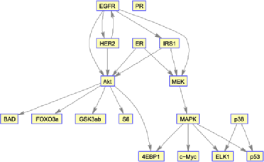
Figure 3: Signaling downstream of the epidermal growth factor receptor (EGFR). The graph shown summarizes known causal links characterized by extensive biochemistry. (Note that edges in the graph represent high-level summaries of often complex molecular interactions that may involve latent chemical species.)

We consider experimental data derived from human breast cancer cell lines, focusing on protein signaling networks within which many (wild type) causal relationships are well understood from extensive biochemistry (Figure 3). The investigation presented below serves three purposes: First, it allows investigation of the applicability of the proposed joint approaches to experimental data. Second, it allows investigation of the use of ancillary information, in the form of mutational status and histological information. Finally, the results and approach are relevant to the topical question of exploring signaling heterogeneity across cancer cell lines.

Data were obtained using reverse-phase protein arrays [Hennessy et al. (2010)] from $J=6$ breast cancer cell lines (AU 565, HCC 1569, MCF 7, MDA MB 231, SKBR3 and SUM 190PT; experimental protocol is described in brief in Supplement A [Oates et al. (2014a)]). Data comprised observations for the $P=17$ proteins shown in Figure 3 (see also STable 1 in the supplementary material [Oates et al. (2014a)]; we note that these data form part of a larger study including further cell lines and proteins). Specifically, $\mathbf{y}$ contains the logarithms of the measured concentrations. Data were acquired under treatment with an EGFR/HER2 inhibitor Lapatinib (“EGFRi”), an Akt inhibitor (“Akti”), EGFRi and Akti in combination, and without inhibition (“DMSO”) at 0.5, 1, 2, 4, 8 and 24 hours following Serum stimulation, giving a total of $n_{j}=24$ observations of each variable in each individual cell line.

4.3.1 Informative priors on causal structure

For the cancer cell lines analyzed here, ancillary information is available in the form of genetic aberrations (mutation statuses) and histological profiling. These were obtained from published sources [Neve et al. (2006)] and online databases [Forbes et al. (2011)] and reproduced in STable 2 (see supplementary material [Oates et al. (2014a)]). These sources give causally relevant information on structure specific to the individual cell lines $j\in\mathcal{J}$. We used this information to help specify priors on the graphs $G^{j}$, considering in particular two cases: (i) Loss-of-function mutations in kinase domains; in line with the nature of the mutation, here we set the prior probability on edges emanating from the mutant protein to zero. Where the mutation is known to also affect the ability of a protein to be phosphorylated, then incoming edges were also assigned zero prior probability. (ii) Cell lines with ectopic expression of the receptor HER2 are known to depend heavily upon EGFR signaling. In this case the network prior did not penalize edges emanating from the EGFR receptor nodes. A full discussion of ancillary data appears in Supplement A [Oates et al. (2014a)].

In addition to the cell-line-specific mutational information above, decades of experimental work (including interventional, biochemical and biophysical studies) have provided a wealth of information about (wild type) causal relationships between nodes. We used this noncell line-specific information to specify a prior graph $G^{0}$ that was common to all cell lines $j\in\mathcal{J}$ (shown in Figure 3). Cancer signaling is expected to differ with respect to wild type signaling, but a priori we expect the differences to be small in number. In light of this observation, we used subjective elicitation (Section 3.3) to set hyperparameters $\lambda=4,\eta=5$, corresponding to $\mathbb{E}(\|G^{j}-G\|)\approx 5$, $\mathbb{E}(\|G-G^{0}\|)\approx 2$.

4.3.2 Validation

In order to test performance, we first considered the latent network $G$, comparing estimates to the (causal) literature network shown in Figure 3. For a fair assessment we used an empty prior network $G^{0}$. Inferred networks are displayed in SFigure 7 (see supplementary material [Oates et al. (2014a)]). Results demonstrated good recovery of the literature network, with J-IDBN attaining the highest AUR (0.67, $p<0.01$, permutation test; Figure 4). As in the simulation study, J-IDBN outperformed IDBN, with AJ-IDBN and Fixed IDBN representing good alternative estimators and the remaining estimators performing poorly. This suggests the conclusions drawn in Section 4.2 apply also to the analysis of biological time series data. In particular, modeling of interventions appears to be crucial in this setting, in line with the conclusions of Spencer, Hill and Mukherjee (2012).

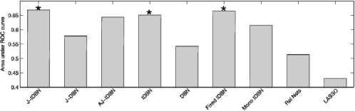
Figure 4: Results from breast cancer cell line data, comparison with network based on literature. The methods shown were used to estimate a latent network; AUR is with respect to the literature-based network shown in Figure 3; the latter was not used to provide prior information in these experiments. (Asterisks denote AUR scores which were significant at the 1% level under a permutation test with AUR as the statistic and $10\mbox{,}000$ samples used to obtain an empirical null distribution.)

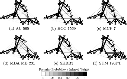
Figure 5: Breast cancer data; cell line-specific networks inferred by J-IDBN. (Edge width and color are proportional to posterior marginal inclusion probabilities. The layout of vertices is congruent to Figure 3, which can be used as a key.)

4.3.3 Inference for cell line networks

We investigated inference for cell line-specific networks $G^{j}$ (Figure 5), taking the prior network $G^{0}$ from the literature (Figure 3). In order to assess results, we exploited the fact that cell lines AU565 and SKBR3 derive from the same patient. We would therefore expect these two cell lines to be most similar at the network level. J-IDBN networks for AU565 and SKBR3 were indeed the most similar, maximizing the Pearson correlation coefficient between corresponding posterior marginal inclusion probabilities over all ${6\choose 2}=15$ pairs of cell lines. In contrast, standard IDBNs did not do so (Figure 6). Figure 7 compares posterior inclusion probabilities (or analogous edge weights for the non-Bayesian methods) for AU565 against SKBR3. We find posterior edge probabilities from these two lines are closer under JNI estimators compared with standard, independent estimators. However, a thorough assessment of the accuracy of the individual cell line-specific networks requires additional experimental work and is beyond the scope of this paper.

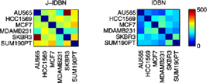
Figure 6: Breast cancer data; pairwise similarity between cell line-specific networks inferred by J-IDBN (left) and IDBN (right). J-IDBN identifies AU 565 and SKBR 3 as having the most similar networks; these cell lines were originally derived from the same patient. In contrast, IDBN does not do so. [Colors denote Bonferroni $-\log(p)$ values based on the Pearson correlation coefficient of posterior inclusion probabilities for pairs of cell lines, so that red indicates a high degree of similarity. For presentation the diagonal is set to zero.]

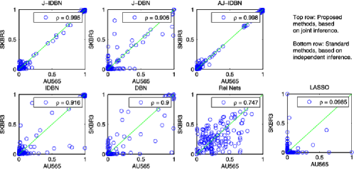
Figure 7: Comparison of posterior edge probabilities obtained from analysis of data from two breast cancer cell lines (AU 565 and SKBR 3) that were originally derived from the same patient. The joint estimators J-IDBN and J-DBN improve the Spearman correlation coefficient (“rho”) between posterior edge probabilities compared to independent inference using IDBN and DBN.

5 Discussion

We focused on three related structure learning problems arising in the context of a set of nonidentical but exchangeable units or individuals:

[(3)]

Estimation of a shared network from the heterogeneous data.

Estimation of networks for specific individuals.

Learning features specific to individuals (“differential networks”). Each problem may be of independent scientific interest; the joint approaches investigated here address all three problems simultaneously within a coherent statistical framework. We considered simulated data, with and without model misspecification, as well as proteomic data obtained from cancer cell lines. For all three problems we demonstrated that a joint analysis performs at least as well as independent or simpler aggregate analyses.

We considered modular priors (that factorize over nodes) that facilitated efficient computation. However, it may be useful to consider richer priors for joint estimation. One possibility that is pertinent to applications in cancer biology would be hierarchical regularization that allows entire pathways to be either active or inactive. However, we note that this would require revisiting hyperparameter elicitation since the heuristics we described are specific to SHD priors. We restricted the joint model to have equal inverse temperatures $\lambda^{1}=\cdots=\lambda^{J}:=\lambda$. Relaxing this assumption may improve robustness to batch effects that target single individuals, since then weak informativeness ($\lambda^{j}\approx 0$) may be learned from data. It would also be interesting to distinguish between $G\setminus G^{j}$ (“loss of function”) and $G^{j}\setminus G$ (“gain of function”) features. In this work we did not explore information sharing through parameter values $\bolds{\theta}^{j}$, yet this may yield more powerful estimators of network structure in settings where individuals’ parameters $\bolds{\theta}^{j},\bolds{\theta}^{k}$ are not independent.

The case of exchangeable networks that we considered here represents the simplest of a more general class of models for related networks. In a sequel to the present paper [Oates and Mukherjee (2014)], we discuss the case where multiple individuals are related according to a known tree structure. In this more general setting, efficient algorithms based on belief propagation continue to apply, since the tree constraint ensures that the corresponding factor graph is acyclic and so the sum-product lemma continues to hold [Kschischang, Frey and Loeliger (2001)]. Still more general (and challenging) is the case where both the networks and the hierarchical structure that relate them to one another are unknown. Oates et al. (2014a, 2014b) present a first step in this direction, in the context of MAP estimation for nonexchangeable DAGs.

Appendix A Proof of Theorem

The following Lemma shows that, under the joint regularity assumption, JNI is a consistent estimator of the true latent network $\overline{G}$ in the limit $J\rightarrow\infty$:

Let $\eta=0$. Then under the joint regularity assumption there exists $0<\varepsilon<1$ such that $\mathbb{E}_{\mathbf{Y},\overline{G},\overline{G^{1}},\ldots,\overline{G^{J}}|\eta,\lambda}p(\overline{G}|\mathbf{Y})>1-|\mathcal{G}|\varepsilon^{J}$.

Since we are using a flat prior ($\eta=0$) on $G$, we have, suppressing dependence upon $\lambda$,

$$p(\overline{G}|\mathbf{Y})=\frac{p(\mathbf{Y}|\overline{G})}{\sum_{G\in\mathcal{G}}p(\mathbf{Y}|G)},$$ (12)

so from Jensen’s inequality

$$\mathbb{E}_{\mathbf{Y},\overline{G^{1}},\ldots,\overline{G^{J}}|\overline{G},\lambda}p(\overline{G}|\mathbf{Y}) \geq \frac{\mathbb{E}_{\mathbf{Y},\overline{G^{1}},\ldots,\overline{G^{J}}|\overline{G},\lambda}p(\mathbf{Y}|\overline{G})}{\sum_{G\in\mathcal{G}}\mathbb{E}_{\mathbf{Y},\overline{G^{1}},\ldots,\overline{G^{J}}|\overline{G},\lambda}p(\mathbf{Y}|G)}$$ (13)

$$= \biggl{[}1+\mathop{\sum_{G\in\mathcal{G}}}_{G\neq\overline{G}}\frac{\mathbb{E}_{\mathbf{Y},\overline{G^{1}},\ldots,\overline{G^{J}}|\overline{G},\lambda}p(\mathbf{Y}|G)}{\mathbb{E}_{\mathbf{Y},\overline{G^{1}},\ldots,\overline{G^{J}}|\overline{G},\lambda}p(\mathbf{Y}|\overline{G})}\biggr{]}^{-1}$$ (14)

$$> 1-\mathop{\sum_{G\in\mathcal{G}}}_{G\neq\overline{G}}\frac{\mathbb{E}_{\mathbf{Y},\overline{G^{1}},\ldots,\overline{G^{J}}|\overline{G},\lambda}p(\mathbf{Y}|G)}{\mathbb{E}_{\mathbf{Y},\overline{G^{1}},\ldots,\overline{G^{J}}|\overline{G},\lambda}p(\mathbf{Y}|\overline{G})}$$ (15)

$$= 1-\mathop{\sum_{G\in\mathcal{G}}}_{G\neq\overline{G}}\prod_{j\in\mathcal{J}}\frac{\mathbb{E}_{\mathbf{Y}^{j},\overline{G^{j}}|\overline{G},\lambda}p(\mathbf{Y}^{j}|G)}{\mathbb{E}_{\mathbf{Y}^{j},\overline{G^{j}}|\overline{G},\lambda}p(\mathbf{Y}^{j}|\overline{G})}.$$ (16)

The joint regularity assumption is equivalent to the requirement that $\mathbb{E}_{\mathbf{Y}^{j},\overline{G^{j}}|\overline{G},\lambda}p(\mathbf{Y}^{j}|G)$ has a unique maximum at $G=\overline{G}$, since

$$\hskip 9.0pt\mathbb{E}_{\mathbf{Y}^{j},\overline{G^{j}}|\overline{G},\lambda}p\bigl{(}\mathbf{Y}^{j}|G\bigr{)} = \mathbb{E}_{\overline{G^{j}}|\overline{G},\lambda}\mathbb{E}_{\mathbf{Y}^{j}|\overline{G^{j}}}\sum_{G^{j}\in\mathcal{G}}p\bigl{(}\mathbf{Y}^{j}|G^{j}\bigr{)}p\bigl{(}G^{j}|G\bigr{)}$$ (17)

$$= \sum_{\overline{G^{j}}\in\mathcal{G}}p\bigl{(}G^{j}|G\bigr{)}\sum_{G^{j}\in\mathcal{G}}\bigl{[}\mathbb{E}_{\mathbf{Y}^{j}|\overline{G^{j}}}p\bigl{(}\mathbf{Y}^{j}|G^{j}\bigr{)}\bigr{]}p\bigl{(}\overline{G^{j}}|\overline{G}\bigr{)}$$ (18)

$$= \sum_{\overline{G^{j}}\in\mathcal{G}}\sum_{G^{j}\in\mathcal{G}}\bigl{(}\mathbf{R}^{T}\bigr{)}_{G,G^{j}}(\mathbf{S})_{G^{j},\overline{G^{j}}}(\mathbf{R})_{\overline{G^{j}},\overline{G}}$$ (19)

$$= \bigl{(}\mathbf{R}^{T}\mathbf{S}\mathbf{R}\bigr{)}_{G,\overline{G}}=(\mathbf{R}\mathbf{S}\mathbf{R})_{G,\overline{G}},$$ (20)

where we have used that $\mathbf{R}$ is symmetric. It follows that

$$\varepsilon:=\mathop{\max_{G\in\mathcal{G}}}_{G\neq\overline{G}}\frac{\mathbb{E}_{\mathbf{Y}^{j},\overline{G^{j}}|\overline{G},\lambda}p(\mathbf{Y}^{j}|G)}{\mathbb{E}_{\mathbf{Y}^{j},\overline{G^{j}}|\overline{G},\lambda}p(\mathbf{Y}^{j}|\overline{G})}<1.$$ (21)

We therefore conclude that

$$\mathbb{E}_{\mathbf{Y},\overline{G^{1}},\ldots,\overline{G^{J}}|\overline{G},\lambda}p(\overline{G}|\mathbf{Y})>1-|\mathcal{G}|\varepsilon^{J}.$$ (22)

Since equation (22) is independent of $\overline{G}$, the result follows.

Proof of Theorem Since no observables are available on the first individual ($\mathbf{Y}^{1}=\varnothing$), we have

$$\mathbf{A}_{\mathrm{JNI}}^{1}=\sum_{G\in\mathcal{G}}p(G|\mathbf{Y})\sum_{G^{1}\in\mathcal{G}}p\bigl{(}G^{1}|G\bigr{)}G^{1}.$$ (23)

We also require the “oracle” estimator (O-JNI); this is simply JNI but with $\overline{G}$ fixed and known, that is,

$$\mathbf{A}_{\mathrm{O\mbox{{-}}JNI}}^{1}=\sum_{G^{1}\in\mathcal{G}}p\bigl{(}G^{1}|\overline{G}\bigr{)}G^{1}.$$ (24)

Note that $\mathbb{E}_{\overline{\mathbf{G}}|\eta,\lambda}\|\mathbf{A}_{\mathrm{O\mbox{{-}}JNI}}^{1}-\overline{G^{1}}\|=\mathbb{E}_{\overline{G^{1}},\overline{G}|\lambda}\|\overline{G}-\overline{G^{1}}\|=P^{2}(1-h_{\lambda})$. We begin by showing that JNI approximates O-JNI:

$$\mathbf{A}_{\mathrm{O\mbox{{-}}JNI}}^{1}-\mathbf{A}_{\mathrm{JNI}}^{1} = \bigl{(}1-p(\overline{G}|\mathbf{Y})\bigr{)}\sum_{G^{1}\in\mathcal{G}}p\bigl{(}G^{1}|\overline{G}\bigr{)}G^{1}$$

$${}-\mathop{\sum_{G\in\mathcal{G}}}_{G\neq\overline{G}}p(G|\mathbf{Y})\sum_{G^{1}\in\mathcal{G}}p\bigl{(}G^{1}|G\bigr{)}G^{1}$$

and, by the triangle inequality,

$$\bigl{\|}\mathbf{A}_{\mathrm{O\mbox{{-}}JNI}}^{1}-\mathbf{A}_{\mathrm{JNI}}^{1}\bigr{\|} \leq \biggl{\|}\bigl{(}1-p(\overline{G}|\mathbf{Y})\bigr{)}\sum_{G^{1}\in\mathcal{G}}p\bigl{(}G^{1}|\overline{G}\bigr{)}G^{1}\biggr{\|}$$ (26)

$${}+\biggl{\|}\mathop{\sum_{G\in\mathcal{G}}}_{G\neq\overline{G}}p(G|\mathbf{Y})\sum_{G^{1}}p\bigl{(}G^{1}|G\bigr{)}G^{1}\biggr{\|}$$

$$\leq \bigl{(}1-p(\overline{G}|\mathbf{Y})\bigr{)}\sup_{G^{1}\in\mathcal{G}}\bigl{\|}G^{1}\bigr{\|}+\bigl{(}1-p(\overline{G}|\mathbf{Y})\bigr{)}\sup_{G^{1}\in\mathcal{G}}\bigl{\|}G^{1}\bigr{\|}$$ (27)

$$\leq 2\bigl{(}1-p(\overline{G}|\mathbf{Y})\bigr{)}P^{2}.$$ (28)

Again, by the triangle inequality,

$$\bigl{\|}\mathbf{A}_{\mathrm{JNI}}^{1}-\overline{G^{1}}\bigr{\|}\leq\bigl{\|}\mathbf{A}_{\mathrm{JNI}}^{1}-\mathbf{A}_{\mathrm{O\mbox{{-}}JNI}}^{1}\bigr{\|}+\bigl{\|}\mathbf{A}_{\mathrm{O\mbox{{-}}JNI}}^{1}-\overline{G^{1}}\bigr{\|}.$$ (29)

Taking expectations and applying the Lemma produces

$$\mathbb{E}_{\mathbf{Y},\overline{\mathbf{G}}|\eta,\lambda}\bigl{\|}\mathbf{A}_{\mathrm{JNI}}^{1}-\overline{G^{1}}\bigr{\|}\leq 2P^{2}|\mathcal{G}|\varepsilon^{J-1}+P^{2}(1-h_{\lambda}),$$ (30)

as required.

Appendix B Dynamic Bayesian networks

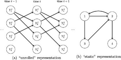
Figure 8: Dynamic Bayesian networks (DBNs). (a) An “unrolled” dynamic Bayesian network (DBN) showing each variable at successive time points. (b) The corresponding “static” representation of DBN (a) with exactly one vertex for each variable.

For the DBNs used here, an edge $(p,q)$ from $p\in\mathcal{P}$ to $q\in\mathcal{P}$ in $G^{j}\in\mathcal{G}$ implies that $Y_{q}^{j}(t)$, the observed value of variable $q$ in individual $j$ at time $t$, depends directly upon $Y_{p}^{j}(t-1)$, the observed value of $p$ in individual $j$ at time $t-1$ [Figure 8(a); note that $t$ indexes the sample index rather than actual sampling time]. Let $\mathbf{Y}^{j}$ denote a vector containing all observations for individual $j$. Then $\mathbf{Y}^{j}(t)$ is conditionally independent of $\{\mathbf{Y}^{j}(t-\tau):\tau\geq 2\}$ given $\mathbf{Y}^{j}(t-1)$, $\bolds{\theta}^{j}$, $G^{j}$ and $Z^{j}$ (first-order Markov assumption). These conditional independence relations are conveniently summarized as a (static) network $G^{j}$ with exactly $P$ vertices [Figure 8(b)]; note that this latter network need not be acyclic.

Hill et al. (2012) describe a DBN rooted in the Bayesian linear model. Specifically, the response $Y_{p}^{j}(t)$ is predicted by covariates $\mathbf{Y}^{j}(t-1)$, that is,

$$\mathbf{Y}_{p}^{j}=\mathbf{X}_{0}\bolds{\alpha}+\mathbf{X}_{\pi_{p}^{j}}^{j}\bolds{\beta}+\bolds{\varepsilon},$$ (31)

where $\bolds{\varepsilon}\sim N(\mathbf{0}_{n\times 1},\sigma^{2}\mathbf{I}_{n\times n})$. In many cases multiple time series will be available. In this case the vector $\mathbf{Y}_{p}^{j}$ contains the concatenated time series. The matrix $\mathbf{X}_{0}=[\mathbf{1}_{\{t=1\}}\enskip\mathbf{1}_{\{t>1\}}]_{n\times 2}$ contains a term for the initial time point in each experiment. The elements of $\mathbf{X}_{\pi_{p}^{j}}^{j}$ corresponding to initial observations $Y_{p}^{j}(1)$ are simply set to zero. Parameters $\bolds{\theta}_{p}^{j}=\{\bolds{\alpha},\bolds{\beta},\sigma\}$ are specific to model $\pi_{p}^{j}$, variable $p$ and individual $j$. In the simplest case, given data $\mathbf{Y}=\mathbf{y}$, the model-specific component $\mathbf{X}_{\pi_{p}^{j}}^{j}$ of the design matrix consists of the raw predictors $\mathbf{y}_{\pi_{p}^{j}}^{j}(t-1)$, where $\mathbf{y}_{Z}^{j}$ denotes the elements of the vector $\mathbf{y}^{j}(t-1)$ belonging to the set $A$, though more complex basis functions may be used, including interaction terms. For experiments performed in this paper, interaction terms were taken to be all possible products of parent variables, following Hill et al. (2012).

Spencer, Hill and Mukherjee (2012) modeled interventional data by modification to the DAG using ideas from causal inference [Pearl (2000)]. We mention briefly some of the key ideas and refer the interested reader to the references for full details. A “perfect intervention” corresponds to 100% removal of the target’s activity with 100% specificity. In the context of protein phosphorylation, kinases may be intervened upon using chemical agents. Spencer, Hill and Mukherjee (2012) make the simplifying assumptions that these interventions are perfect [the “perfect out fixed effects” (POFE) approach]. We refer the reader to Spencer, Hill and Mukherjee (2012) for an extended discussion of POFE. This changes the DAG structure to model the intervention and also estimates an additional fixed effect parameter to model the change under intervention in the log-transformed data. When generating data for the simulation study in Section 4.2 we take fixed effects to equal zero.

Appendix C Exact marginal likelihood for DBN and IDBN

Hill et al. (2012) employed an exact Bayesian approach to capture the suitability of the candidate parent set $\pi_{p}^{j}$. In brief, a Jeffreys prior $p(\bolds{\alpha},\sigma|\pi_{p}^{j},\phi^{j},\break Z^{j})\propto 1/\sigma$ for $\sigma>0$ was placed over the common parameters. Prior to inference, the noninterventional components of the design matrix are orthogonalized using the transformation $(\mathbf{X}_{\pi_{p}^{j}}^{j})_{ik}\mapsto\sum_{l}(\mathbf{I}_{n}-\mathbf{P}_{0})_{il}(\mathbf{X}_{\pi_{p}^{j}}^{j})_{lk}$, where $\mathbf{P}_{0}=\mathbf{X}_{0}(\mathbf{X}_{0}^{T}\mathbf{X}_{0})^{-1}\mathbf{X}_{0}^{T}$ [Bayarri et al. (2012)]. A $g$-prior was placed on regression coefficients [Zellner (1986)], given by

$$\bolds{\beta}|\bolds{\alpha},\sigma,\pi_{p}^{j},\phi^{j},Z^{j}\sim N\bigl{(}\mathbf{0}_{b\times 1},\phi^{j}\sigma^{2}\bigl{(}\mathbf{X}_{\pi_{p}^{j}}^{T}\mathbf{X}_{\pi_{p}^{j}}\bigr{)}^{-1}\bigr{)},$$ (32)

where $b=\dim(\bolds{\beta})$. Using these priors alongside either DBNs or IDBNs as outlined above, the marginal likelihood can be obtained in closed-form:

$$\mathfrak{P}\bigl{(}\mathbf{y}_{p}^{j}|\pi_{p}^{j},\phi^{j},Z^{j}\bigr{)}$$

(33)

$$\qquad\propto\frac{1}{(\phi^{j}+1)^{b/2}}\biggl{(}\mathbf{y}_{p}^{jT}\biggl{(}\mathbf{I}_{n\times n}-\mathbf{P}_{0}-\frac{\phi^{j}}{\phi^{j}+1}\mathbf{P}_{\pi_{p}^{j}}\biggr{)}\mathbf{y}_{p}^{j}\biggr{)}^{-({n-a})/{2}},$$

where $\mathbf{P}_{\pi_{p}^{j}}=\mathbf{X}_{\pi_{p}^{j}}(\mathbf{X}_{\pi_{p}^{j}}^{T}\mathbf{X}_{\pi_{p}^{j}})^{-1}\mathbf{X}_{\pi_{p}^{j}}^{T}$, $a=\dim(\bolds{\alpha})$ and $b=\dim(\bolds{\beta})$. Empirical investigations have previously demonstrated good results for network inference based on the above marginal likelihood [Hill et al. (2012), Spencer, Hill and Mukherjee (2012)].

The hyperparameter $\phi^{j}$, that is related to the weight of the parameter prior $p(\bolds{\beta}|\bolds{\alpha},\sigma)$ relative to the data $\mathbf{y}_{p}^{j}$, was selected in this paper using the conditional empirical Bayes procedure outlined in George and Foster (2000), corresponding to

$$\hat{\phi}^{j}\bigl{(}\pi_{p}^{j}\bigr{)}={\arg\max}_{g}\mathfrak{P}\bigl{(}\mathbf{y}_{p}^{j}|\pi_{p}^{j},g,Z^{j}\bigr{)}.$$ (34)

For computational efficiency, we evaluated the argument over a set of eight candidate values corresponding to prior weights of 0, 10, 20, 30, 40, 50% and $(100/n)\%$ (the unit information prior). Alternative strategies for eliciting $g$-priors are discussed in Bayarri et al. (2012), Liang et al. (2008).

Appendix D Belief propagation for JNI

Exact inference for JNI is based on belief propagation [Pearl (2000)]. Algorithm 1 displays pseudocode for exact joint model averaging. We also indicate computational complexity in terms of the number $M=|\mathcal{G}_{p}|$ of possible parent sets and the number $J$ of individuals. Computational complexity of calculating marginal likelihoods $\mathfrak{P}(\mathbf{y}_{p}^{j}|\pi_{p}^{j})$ will partly depend upon sample size $n$; scaling exponents shown here assume $\mathcal{O}(n)=\mathcal{O}(1)$. Algorithm 1 contains pseudocode for computation of posterior marginal inclusion probabilities for edges in both the latent network $G$ and individual-specific networks $G^{j}$. For simplicity, we suppress dependence upon ancillary data $Z^{j}$ throughout.

Algorithm 1 Belief propagation for JNI

1:for $p\in\mathcal{P}$ do

2:

3:     Compute and cache $\mathfrak{P}(\mathbf{y}_{p}^{j}|\pi_{p}^{j})$ [$\forall j\in\mathcal{J}$] [$\forall\pi_{p}\in\mathcal{G}_{p}$]

4:

5:     Compute and cache [$\forall j\in\mathcal{J}$] [$\forall\pi_{p}\in\mathcal{G}_{p}$]

6:     $\mathfrak{P}(\mathbf{y}_{p}^{j}|\pi_{p})=\sum_{\pi_{p}^{j}\in\mathcal{G}_{p}}\mathfrak{P}(\mathbf{y}_{p}^{j}|\pi_{p}^{j})p(\pi_{p}^{j}|\pi_{p})$ [$\mathcal{O}(M)$]

7:

8:     Compute and cache [$\forall j\in\mathcal{J}$] [$\forall\pi_{p},\pi_{p}^{j}\in\mathcal{G}_{p}$]

9:     $p(\pi_{p}|\mathbf{y}_{p},\pi_{p}^{0})\propto p(\pi_{p}|\pi_{p}^{0})\prod_{j\in\mathcal{J}}\mathfrak{P}(\mathbf{y}_{p}^{j}|\pi_{p})$ [$\mathcal{O}(J)$]

10:     $p(\pi_{p}^{j}|\mathbf{y}_{p},\pi_{p}^{0})\propto\sum_{\pi_{p}\in\mathcal{G}_{p}}p(\pi_{p}|\pi_{p}^{0})\mathfrak{P}(\mathbf{y}_{p}^{j}|\pi_{p}^{j})p(\pi_{p}^{j}|\pi_{p})\prod_{k\in\mathcal{J}\setminus\{j\}}\mathfrak{P}(\mathbf{y}_{p}^{k}|\pi_{p})[\mathcal{O}(MJ)$]

11:

12:     Compute and cache [$\forall j\in\mathcal{J}$] [$\forall i\in\mathcal{P}$]

13:     $p(i\in\pi_{p}|\mathbf{y},G^{0})=\sum_{\pi_{p}\in\mathcal{G}_{p}}\mathbf{1}_{i\in\pi_{p}}p(\pi_{p}|\mathbf{y}_{p},\pi_{p}^{0})$ [$\mathcal{O}(M)$]

14:     $p(i\in\pi_{p}^{j}|\mathbf{y},G^{0})=\sum_{\pi_{p}^{j}\in\mathcal{G}_{p}}\mathbf{1}_{i\in\pi_{p}^{j}}p(\pi_{p}^{j}|\mathbf{y},\pi_{p}^{0})$ [$\mathcal{O}(M)$]

15:end for

References

- The 1000 Genomes Project Consortium (2010) {barticle}[pbm] \bauthor\bsnmThe 1000 Genomes Project Consortium (\byear2010). \btitleA map of human genome variation from population-scale sequencing. \bjournalNature \bvolume467 \bpages1061–1073. \biddoi=10.1038/nature09534, issn=1476-4687, mid=UKMS34220, pii=nature09534, pmcid=3042601, pmid=20981092 \bptokimsref\endbibitem
- Akbani et al. (2014) {barticle}[auto] \bauthor\bsnmAkbani, \bfnmR.\binitsR. \betalet al. (\byear2014). \btitleA pan-cancer proteomic perspective on the Cancer Genome Atlas. \bjournalNat. Commun. \bvolume5 \bpages3887. \bptokimsref\endbibitem
- Barretina et al. (2012) {barticle}[pbm] \bauthor\bsnmBarretina, \bfnmJordi\binitsJ., \bauthor\bsnmCaponigro, \bfnmGiordano\binitsG., \bauthor\bsnmStransky, \bfnmNicolas\binitsN., \bauthor\bsnmVenkatesan, \bfnmKavitha\binitsK., \bauthor\bsnmMargolin, \bfnmAdam A.\binitsA. A., \bauthor\bsnmKim, \bfnmSungjoon\binitsS., \bauthor\bsnmWilson, \bfnmChristopher J.\binitsC. J., \bauthor\bsnmLehár, \bfnmJoseph\binitsJ., \bauthor\bsnmKryukov, \bfnmGregory V.\binitsG. V., \bauthor\bsnmSonkin, \bfnmDmitriy\binitsD., \bauthor\bsnmReddy, \bfnmAnupama\binitsA., \bauthor\bsnmLiu, \bfnmManway\binitsM., \bauthor\bsnmMurray, \bfnmLauren\binitsL., \bauthor\bsnmBerger, \bfnmMichael F.\binitsM. F., \bauthor\bsnmMonahan, \bfnmJohn E.\binitsJ. E., \bauthor\bsnmMorais, \bfnmPaula\binitsP., \bauthor\bsnmMeltzer, \bfnmJodi\binitsJ., \bauthor\bsnmKorejwa, \bfnmAdam\binitsA., \bauthor\bsnmJané-Valbuena, \bfnmJudit\binitsJ., \bauthor\bsnmMapa, \bfnmFelipa A.\binitsF. A., \bauthor\bsnmThibault, \bfnmJoseph\binitsJ., \bauthor\bsnmBric-Furlong, \bfnmEva\binitsE., \bauthor\bsnmRaman, \bfnmPichai\binitsP., \bauthor\bsnmShipway, \bfnmAaron\binitsA., \bauthor\bsnmEngels, \bfnmIngo H.\binitsI. H., \bauthor\bsnmCheng, \bfnmJill\binitsJ., \bauthor\bsnmYu, \bfnmGuoying K.\binitsG. K., \bauthor\bsnmYu, \bfnmJianjun\binitsJ., \bauthor\bsnmPeter Aspesi, \bfnmJr\binitsJ., \bauthor\bparticlede \bsnmSilva, \bfnmMelanie\binitsM., \bauthor\bsnmJagtap, \bfnmKalpana\binitsK., \bauthor\bsnmJones, \bfnmMichael D.\binitsM. D., \bauthor\bsnmWang, \bfnmLi\binitsL., \bauthor\bsnmHatton, \bfnmCharles\binitsC., \bauthor\bsnmPalescandolo, \bfnmEmanuele\binitsE., \bauthor\bsnmGupta, \bfnmSupriya\binitsS., \bauthor\bsnmMahan, \bfnmScott\binitsS., \bauthor\bsnmSougnez, \bfnmCarrie\binitsC., \bauthor\bsnmOnofrio, \bfnmRobert C.\binitsR. C., \bauthor\bsnmLiefeld, \bfnmTed\binitsT., \bauthor\bsnmMacConaill, \bfnmLaura\binitsL., \bauthor\bsnmWinckler, \bfnmWendy\binitsW., \bauthor\bsnmReich, \bfnmMichael\binitsM., \bauthor\bsnmLi, \bfnmNanxin\binitsN., \bauthor\bsnmMesirov, \bfnmJill P.\binitsJ. P., \bauthor\bsnmGabriel, \bfnmStacey B.\binitsS. B., \bauthor\bsnmGetz, \bfnmGad\binitsG., \bauthor\bsnmArdlie, \bfnmKristin\binitsK., \bauthor\bsnmChan, \bfnmVivien\binitsV., \bauthor\bsnmMyer, \bfnmVic E.\binitsV. E., \bauthor\bsnmWeber, \bfnmBarbara L.\binitsB. L., \bauthor\bsnmPorter, \bfnmJeff\binitsJ., \bauthor\bsnmWarmuth, \bfnmMarkus\binitsM., \bauthor\bsnmFinan, \bfnmPeter\binitsP., \bauthor\bsnmHarris, \bfnmJennifer L.\binitsJ. L., \bauthor\bsnmMeyerson, \bfnmMatthew\binitsM., \bauthor\bsnmGolub, \bfnmTodd R.\binitsT. R., \bauthor\bsnmMorrissey, \bfnmMichael P.\binitsM. P., \bauthor\bsnmSellers, \bfnmWilliam R.\binitsW. R., \bauthor\bsnmSchlegel, \bfnmRobert\binitsR. and \bauthor\bsnmGarraway, \bfnmLevi A.\binitsL. A. (\byear2012). \btitleThe Cancer Cell Line Encyclopedia enables predictive modelling of anticancer drug sensitivity. \bjournalNature \bvolume483 \bpages603–607. \biddoi=10.1038/nature11003, issn=1476-4687, mid=NIHMS361223, pii=nature11003, pmcid=3320027, pmid=22460905 \bptokimsref\endbibitem
- Bayarri et al. (2012) {barticle}[mr] \bauthor\bsnmBayarri, \bfnmM. J.\binitsM. J., \bauthor\bsnmBerger, \bfnmJ. O.\binitsJ. O., \bauthor\bsnmForte, \bfnmA.\binitsA. and \bauthor\bsnmGarcía-Donato, \bfnmG.\binitsG. (\byear2012). \btitleCriteria for Bayesian model choice with application to variable selection. \bjournalAnn. Statist. \bvolume40 \bpages1550–1577. \biddoi=10.1214/12-AOS1013, issn=0090-5364, mr=3015035 \bptokimsref\endbibitem
- Boutilier et al. (1996) {bincollection}[mr] \bauthor\bsnmBoutilier, \bfnmCraig\binitsC., \bauthor\bsnmFriedman, \bfnmNir\binitsN., \bauthor\bsnmGoldszmidt, \bfnmMoises\binitsM. and \bauthor\bsnmKoller, \bfnmDaphne\binitsD. (\byear1996). \btitleContext-specific independence in Bayesian networks. In \bbooktitleUncertainty in Artificial Intelligence (Portland, OR, 1996) \bpages115–123. \bpublisherMorgan Kaufmann, \blocationSan Francisco, CA. \bidmr=1617129 \bptokimsref\endbibitem
- Butte et al. (2000) {barticle}[pbm] \bauthor\bsnmButte, \bfnmA. J.\binitsA. J., \bauthor\bsnmTamayo, \bfnmP.\binitsP., \bauthor\bsnmSlonim, \bfnmD.\binitsD., \bauthor\bsnmGolub, \bfnmT. R.\binitsT. R. and \bauthor\bsnmKohane, \bfnmI. S.\binitsI. S. (\byear2000). \btitleDiscovering functional relationships between RNA expression and chemotherapeutic susceptibility using relevance networks. \bjournalProc. Natl. Acad. Sci. USA \bvolume97 \bpages12182–12186. \biddoi=10.1073/pnas.220392197, issn=0027-8424, pii=220392197, pmcid=17315, pmid=11027309 \bptokimsref\endbibitem
- The Cancer Genome Atlas Network (2012) {barticle}[auto] \bauthor\bsnmThe Cancer Genome Atlas Network (\byear2012). \btitleComprehensive molecular portraits of human breast tumours. \bjournalNature \bvolume490 \bpages61–70. \bptokimsref\endbibitem
- Cao et al. (2011) {barticle}[pbm] \bauthor\bsnmCao, \bfnmJun\binitsJ., \bauthor\bsnmSchneeberger, \bfnmKorbinian\binitsK., \bauthor\bsnmOssowski, \bfnmStephan\binitsS., \bauthor\bsnmGünther, \bfnmTorsten\binitsT., \bauthor\bsnmBender, \bfnmSebastian\binitsS., \bauthor\bsnmFitz, \bfnmJoffrey\binitsJ., \bauthor\bsnmKoenig, \bfnmDaniel\binitsD., \bauthor\bsnmLanz, \bfnmChrista\binitsC., \bauthor\bsnmStegle, \bfnmOliver\binitsO., \bauthor\bsnmLippert, \bfnmChristoph\binitsC., \bauthor\bsnmWang, \bfnmXi\binitsX., \bauthor\bsnmOtt, \bfnmFelix\binitsF., \bauthor\bsnmMüller, \bfnmJonas\binitsJ., \bauthor\bsnmAlonso-Blanco, \bfnmCarlos\binitsC., \bauthor\bsnmBorgwardt, \bfnmKarsten\binitsK., \bauthor\bsnmSchmid, \bfnmKarl J.\binitsK. J. and \bauthor\bsnmWeigel, \bfnmDetlef\binitsD. (\byear2011). \btitleWhole-genome sequencing of multiple Arabidopsis thaliana populations. \bjournalNat. Genet. \bvolume43 \bpages956–963. \biddoi=10.1038/ng.911, issn=1546-1718, pii=ng.911, pmid=21874002 \bptokimsref\endbibitem
- Curtis et al. (2012) {barticle}[auto] \bauthor\bsnmCurtis, \bfnmC.\binitsC. \betalet al. (\byear2012). \btitleThe genomic and transcriptomic architecture of 2,000 breast tumours reveals novel subgroups. \bjournalNature \bvolume486 \bpages346–352. \bptokimsref\endbibitem
- Danaher, Wang and Witten (2014) {barticle}[mr] \bauthor\bsnmDanaher, \bfnmPatrick\binitsP., \bauthor\bsnmWang, \bfnmPei\binitsP. and \bauthor\bsnmWitten, \bfnmDaniela M.\binitsD. M. (\byear2014). \btitleThe joint graphical lasso for inverse covariance estimation across multiple classes. \bjournalJ. R. Stat. Soc. Ser. B Stat. Methodol. \bvolume76 \bpages373–397. \biddoi=10.1111/rssb.12033, issn=1369-7412, mr=3164871 \bptokimsref\endbibitem
- Dondelinger, Lèbre and Husmeier (2013) {barticle}[mr] \bauthor\bsnmDondelinger, \bfnmFrank\binitsF., \bauthor\bsnmLèbre, \bfnmSophie\binitsS. and \bauthor\bsnmHusmeier, \bfnmDirk\binitsD. (\byear2013). \btitleNon-homogeneous dynamic Bayesian networks with Bayesian regularization for inferring gene regulatory networks with gradually time-varying structure. \bjournalMach. Learn. \bvolume90 \bpages191–230. \biddoi=10.1007/s10994-012-5311-x, issn=0885-6125, mr=3015742 \bptnotecheck year \bptokimsref\endbibitem
- Forbes et al. (2011) {barticle}[auto] \bauthor\bsnmForbes, \bfnmS. A.\binitsS. A. \betalet al. (\byear2011). \btitleCOSMIC: Mining complete cancer genomes in the catalogue of somatic mutations in cancer. \bjournalNucleic Acids Res. \bvolume39 \bpagesD945–D950. \bptokimsref\endbibitem
- Geiger and Heckerman (1996) {barticle}[mr] \bauthor\bsnmGeiger, \bfnmDan\binitsD. and \bauthor\bsnmHeckerman, \bfnmDavid\binitsD. (\byear1996). \btitleKnowledge representation and inference in similarity networks and Bayesian multinets. \bjournalArtificial Intelligence \bvolume82 \bpages45–74. \biddoi=10.1016/0004-3702(95)00014-3, issn=0004-3702, mr=1391056 \bptokimsref\endbibitem
- George and Foster (2000) {barticle}[mr] \bauthor\bsnmGeorge, \bfnmEdward I.\binitsE. I. and \bauthor\bsnmFoster, \bfnmDean P.\binitsD. P. (\byear2000). \btitleCalibration and empirical Bayes variable selection. \bjournalBiometrika \bvolume87 \bpages731–747. \biddoi=10.1093/biomet/87.4.731, issn=0006-3444, mr=1813972 \bptokimsref\endbibitem
- Hennessy et al. (2010) {barticle}[auto] \bauthor\bsnmHennessy, \bfnmB. T.\binitsB. T. \betalet al. (\byear2010). \btitleA technical assessment of the utility of reverse phase protein arrays for the study of the functional proteome in nonmicrodissected human breast cancer. \bjournalClin. Proteom. \bvolume6 \bpages129–151. \bptokimsref\endbibitem
- Hill et al. (2012) {barticle}[auto] \bauthor\bsnmHill, \bfnmS. M.\binitsS. M. \betalet al. (\byear2012). \btitleBayesian inference of signaling network topology in a cancer cell line. \bjournalBioinformatics \bvolume28 \bpages2804–2810. \bptokimsref\endbibitem
- Ibrahim and Chen (2000) {barticle}[mr] \bauthor\bsnmIbrahim, \bfnmJoseph G.\binitsJ. G. and \bauthor\bsnmChen, \bfnmMing-Hui\binitsM.-H. (\byear2000). \btitlePower prior distributions for regression models. \bjournalStatist. Sci. \bvolume15 \bpages46–60. \biddoi=10.1214/ss/1009212673, issn=0883-4237, mr=1842236 \bptokimsref\endbibitem
- Ideker and Krogan (2012) {barticle}[pbm] \bauthor\bsnmIdeker, \bfnmTrey\binitsT. and \bauthor\bsnmKrogan, \bfnmNevan J.\binitsN. J. (\byear2012). \btitleDifferential network biology. \bjournalMol. Syst. Biol. \bvolume8 \bpages565. \biddoi=10.1038/msb.2011.99, issn=1744-4292, pii=msb201199, pmcid=3296360, pmid=22252388 \bptokimsref\endbibitem
- Imoto et al. (2003) {bincollection}[auto] \bauthor\bsnmImoto, \bfnmS.\binitsS. \betalet al. (\byear2003). \btitleCombining microarrays and biological knowledge for estimating gene networks via Bayesian networks. In \bseriesProceedings of the IEEE Computer Society Bioinformatics Conference \bpages104-113. \bptokimsref\endbibitem
- Kschischang, Frey and Loeliger (2001) {barticle}[mr] \bauthor\bsnmKschischang, \bfnmFrank R.\binitsF. R., \bauthor\bsnmFrey, \bfnmBrendan J.\binitsB. J. and \bauthor\bsnmLoeliger, \bfnmHans-Andrea\binitsH.-A. (\byear2001). \btitleFactor graphs and the sum-product algorithm. \bjournalIEEE Trans. Inform. Theory \bvolume47 \bpages498–519. \biddoi=10.1109/18.910572, issn=0018-9448, mr=1820474 \bptokimsref\endbibitem
- Liang et al. (2008) {barticle}[mr] \bauthor\bsnmLiang, \bfnmFeng\binitsF., \bauthor\bsnmPaulo, \bfnmRui\binitsR., \bauthor\bsnmMolina, \bfnmGerman\binitsG., \bauthor\bsnmClyde, \bfnmMerlise A.\binitsM. A. and \bauthor\bsnmBerger, \bfnmJim O.\binitsJ. O. (\byear2008). \btitleMixtures of priors for Bayesian variable selection. \bjournalJ. Amer. Statist. Assoc. \bvolume103 \bpages410–423. \biddoi=10.1198/016214507000001337, issn=0162-1459, mr=2420243 \bptokimsref\endbibitem
- Maher (2012) {barticle}[pbm] \bauthor\bsnmMaher, \bfnmBrendan\binitsB. (\byear2012). \btitleENCODE: The human encyclopaedia. \bjournalNature \bvolume489 \bpages46–48. \bidissn=1476-4687, pmid=22962707 \bptokimsref\endbibitem
- Mukherjee and Speed (2008) {barticle}[pbm] \bauthor\bsnmMukherjee, \bfnmSach\binitsS. and \bauthor\bsnmSpeed, \bfnmTerence P.\binitsT. P. (\byear2008). \btitleNetwork inference using informative priors. \bjournalProc. Natl. Acad. Sci. USA \bvolume105 \bpages14313–14318. \biddoi=10.1073/pnas.0802272105, issn=1091-6490, pii=0802272105, pmcid=2567188, pmid=18799736 \bptokimsref\endbibitem
- Murphy (2002) {bmisc}[auto] \bauthor\bsnmMurphy, \bfnmKevin Patrick\binitsK. P. (\byear2002). \bhowpublishedDynamic Bayesian networks: Representation, inference and learning. Ph.D. thesis, California Univ., Berkeley. \bidmr=2704368 \bptokimsref\endbibitem
- Neve et al. (2006) {barticle}[auto] \bauthor\bsnmNeve, \bfnmR. M.\binitsR. M. \betalet al. (\byear2006). \btitleA collection of breast cancer cell lines for the study of functionally distinct cancer subtypes. \bjournalCancer Cell \bvolume10 \bpages515–527. \bptokimsref\endbibitem
- Niculescu-Mizil and Caruana (2007) {barticle}[author] \bauthor\bsnmNiculescu-Mizil, \bfnmA.\binitsA. and \bauthor\bsnmCaruana, \bfnmR.\binitsR. (\byear2007). \btitleInductive transfer for Bayesian network structure learning. \bjournalJ. Mach. Learn. Res. Workshop and Conference Proceedings \bvolume27 \bpages339–346. \bptokimsref\endbibitem
- Oates and Mukherjee (2014) {barticle}[auto] \bauthor\bsnmOates, \bfnmC. J.\binitsC. J. and \bauthor\bsnmMukherjee, \bfnmS.\binitsS. (\byear2014). \btitleJoint structure learning of multiple non-exchangeable networks. \bjournalJ. Mach. Learn. Res. Workshop and Conference Proceedings \bvolume33 \bpages687–695. \bnoteIn Proceedings of the Seventeenth International Conference on Artificial Intelligence and Statistics (AISTATS 2014). \bptokimsref\endbibitem
- Oates, Costa and Nichols (2014) {bmisc}[auto] \bauthor\bsnmOates, \bfnmC. J.\binitsC. J., \bauthor\bsnmCosta, \bfnmL.\binitsL. and \bauthor\bsnmNichols, \bfnmT. E.\binitsT. E. (\byear2014). \bhowpublishedTowards a multi-subject analysis of neural connectivity. Neural Comput. To appear. \bptokimsref\endbibitem
- Oates et al. (2014a) {bmisc}[author] \bauthor\bsnmOates, \binitsC. J., \bauthor\bsnmKorkola, \binitsJ. \bauthor\bsnmGray, \binitsJ. W. and \bauthor\bsnmMukherjee, \binitsS. (\byear2014a). \bhowpublishedSupplement to “Joint estimation of multiple related biological networks.” DOI:\doiurl10.1214/14-AOAS761SUPPA. \bptokimsref \endbibitem
- Oates et al. (2014b) {bmisc}[author] \bauthor\bsnmOates, \binitsC. J., \bauthor\bsnmKorkola, \binitsJ. \bauthor\bsnmGray, \binitsJ. W. and \bauthor\bsnmMukherjee, \binitsS. (\byear2014b). \bhowpublishedSupplement to “Joint estimation of multiple related biological networks.” DOI:\doiurl10.1214/14-AOAS761SUPPB. \bptokimsref \endbibitem
- Oyen and Lane (2013) {bincollection}[auto] \bauthor\bsnmOyen, \bfnmD.\binitsD. and \bauthor\bsnmLane, \bfnmT.\binitsT. (\byear2013). \btitleBayesian discovery of multiple Bayesian networks via transfer learning. In \bseriesIEEE Thirteenth International Conference on Data Mining (ICDM) \bpages577–586. \bpublisherIEEE, \blocationDallas. \bptokimsref\endbibitem
- Pearl (1982) {bincollection}[auto] \bauthor\bsnmPearl, \bfnmJ.\binitsJ. (\byear1982). \btitleReverend bayes on inference engines: A distributed tree approach. In \bseriesProceedings of the Second National Conference on Artificial Intelligence \bpages133–136. \blocationPittsburg. \bptokimsref\endbibitem
- Pearl (2000) {bbook}[mr] \bauthor\bsnmPearl, \bfnmJudea\binitsJ. (\byear2000). \btitleCausality: Models, Reasoning, and Inference. \bpublisherCambridge Univ. Press, \blocationCambridge. \bidmr=1744773 \bptokimsref\endbibitem
- Penfold et al. (2012) {barticle}[pbm] \bauthor\bsnmPenfold, \bfnmChristopher A.\binitsC. A., \bauthor\bsnmBuchanan-Wollaston, \bfnmVicky\binitsV., \bauthor\bsnmDenby, \bfnmKatherine J.\binitsK. J. and \bauthor\bsnmWild, \bfnmDavid L.\binitsD. L. (\byear2012). \btitleNonparametric Bayesian inference for perturbed and orthologous gene regulatory networks. \bjournalBioinformatics \bvolume28 \bpagesi233–i241. \biddoi=10.1093/bioinformatics/bts222, issn=1367-4811, pii=bts222, pmcid=3371854, pmid=22689766 \bptokimsref\endbibitem