Variance optimal hedging for continuous time additive processes and applications

Abstract

For a large class of vanilla contingent claims, we establish an explicit Föllmer-Schweizer decomposition when the underlying is an exponential of an additive process. This allows to provide an efficient algorithm for solving the mean variance hedging problem. Applications to models derived from the electricity market are performed.

Key words and phrases: Variance-optimal hedging, Föllmer-Schweizer decomposition, Lévy’s processes, Electricity markets, Processes with independent increments, Additive processes.

2000 AMS-classification: 60G51, 60H05, 60J25, 60J75

1 Introduction

There are basically two main approaches to define the mark to market of a contingent claim: one relying on the no-arbitrage assumption and the other related to a hedging portfolio, those two approaches converging in the specific case of complete markets. In this paper we focus on the hedging approach. A simple introduction to the different hedging and pricing models in incomplete markets can be found in chapter 10 of [13].
When the market is not complete, it is not possible, in general, to hedge perfectly an option. One has to specify risk criteria, and consider the hedging strategy that minimizes the distance (in terms of the given criteria) between the payoff of the option and the terminal value of the hedging portfolio. In practice the price of the option is related to two components: first, the initial-capital value and second the quantitative evaluation of the residual risk induced by this imperfect hedging strategy (due to incompleteness).
Several criteria can be adopted. The aim of super-hedging is to hedge all cases. This approach yields in general prices that are too expensive to be realistic [18]. Quantile hedging modifies this approach allowing for a limited probability of loss [20]. Indifference utility pricing introduced in [23] defines the price of an option to sell (resp. to buy) as the minimum initial value s.t. the hedging portfolio with the option sold (resp. bought) is equivalent (in term of utility) to the initial portfolio. Global quadratic hedging approach was developed by M. Schweizer ([38], [40]): the distance defined by the expectation of the square of the difference between the hedging portfolio and the payoff is minimized. Then, contrarily to the case of utility maximization, in general that approach provides linear prices and hedge ratios with respect to the payoff.

In this paper, we follow this last approach either to derive the hedging strategy minimizing the global quadratic hedging error for a given initial capital, or to derive both the initial capital and the hedging strategy minimizing the same error. Both actions are referred to the objective measure. Moreover we also derive explicit formulae for the global quadratic hedging error which together with the initial capital allows the practitioner to define his option price.

We spend now some words related to the global quadratic hedging approach which is also called mean-variance hedging or global risk minimization. Given a square integrable r.v. $H$, we say that the pair $(V_{0},\varphi)$ is optimal if $(c,v)=(V_{0},\varphi)$ minimizes the functional $\mathbb{E}\left(H-c-\int_{0}^{T}vdS\right)^{2}$. The quantity $V_{0}$ and process $\varphi$ represent the initial capital and the optimal hedging strategy of the contingent claim $H$.

Technically speaking, the global risk minimization problem is based on the local risk minimization one which is strictly related to the so-called Föllmer-Schweizer decomposition (or FS decomposition) of a square integrable random variable (representing the contingent claim) with respect to an $({\cal F}_{t})$-semimartingale $S=M+A$ modeling the asset price: $M$ is an $({\cal F}_{t})$-local martingale and $A$ is a bounded variation process with $A_{0}=0$. Mathematically, the FS decomposition, constitutes the generalization of the martingale representation theorem (Kunita-Watanabe representation), which is valid when $S$ is a Brownian motion or a martingale. Given a square integrable random variable $H$, the problem consists in expressing $H$ as $H_{0}+\int_{0}^{T}\xi dS+L_{T}$ where $\xi$ is predictable and $L_{T}$ is the terminal value of an orthogonal martingale $L$ to $M$, i.e. the martingale part of $S$. In the seminal paper [21], the problem is treated for an underlying process $S$ with continuous paths. In the general case, $S$ is said to satisfy the structure condition (SC) if there is a predictable process $\alpha$ such that $A_{t}=\int_{0}^{t}\alpha_{s}d\langle M\rangle_{s}$ and $\int_{0}^{T}\alpha_{s}^{2}d\langle M\rangle_{s}<\infty$ a.s. In the sequel, most of the contributions were produced in the multidimensional case. Here, for simplicity, we will formulate all the results in the one-dimensional case.

$H_{0}$ constitutes in fact the initial capital and it is given by the expectation of $H$ under the so called variance optimal signed measure (VOM). Hence, in full generality, the initial capital $V_{0}$ is not guaranteed to be an arbitrage-free price. For continuous processes, the variance optimal measure is proved to be non-negative under a mild no-arbitrage condition [41]. Arai ([4] and [3]) provides sufficient conditions for the variance-optimal martingale measure to be a probability measure, even for discontinuous semimartingales.
In the framework of FS decomposition, a process which plays a significant role is the so-called mean variance trade-off (MVT) process $K$. This notion is inspired by the theory in discrete time started by [36]; under condition (SC), in the continuous time case $K$ is defined as $K_{t}=\int_{0}^{t}\alpha^{2}_{s}d\langle M\rangle_{s},\ t\in[0,T]$. In fact, in [38] also appear a slight more general condition, called (ESC), together with a corresponding EMVT process; we will nevertheless not discuss here further details. If the MVT process is deterministic, [38] solves the mean-variance hedging problem and also provides an efficient relation between the solution of the global risk minimization problem and the FS decomposition, see Theorem 4.1. We remark that, in the continuous case, treated by [21], no need of any condition on $K$ is required. It also shows that, for obtaining the mentioned relation, previous condition is not far from being optimal. The next important step was done in [30] where, under the only condition that $K$ is uniformly bounded, the FS decomposition of any square integrable random variable exists, it is unique and the global minimization problem admits a solution.
More recently has appeared an incredible amount of papers in the framework of global (resp. local) risk minimization, so that it is impossible to list all of them and it is beyond our scope. Four significant papers containing a good list of references are [42], [7], [11] and [43].

In this paper, we are not interested in generalizing the conditions under which the FS decomposition exists. The present article aims, in the spirit of a simplified Clark-Ocone formula, at providing an explicit form for the FS decomposition for a large class of European payoffs $H$, when the process $S$ is an exponential of additive process which is not necessarily a martingale. From a practical point of view, this serves to compute efficiently the variance optimal hedging strategy which is directly related to the FS decomposition, since the mean-variance trade-off is for that type of processes deterministic. One major idea proposed by Hubalek, Kallsen and Krawczyk in [24], in the case where the log price is a Lévy process, consists in determining an explicit expression for the variance optimal hedging strategy for exponential payoffs and then deriving, by linear combination the corresponding optimal strategy for a large class of payoff functions (through Laplace type transform). Using the same idea, this paper extends results of [24] considering prices that are exponential of additive processes and contingent claims that are Laplace-Fourier transform of a finite measure. In this generalized framework, we could formulate assumptions as general as possible. In particular, our results do not require any assumption on the absolute continuity of the cumulant generating function of $\log(S_{t})$, thanks to the use of a natural reference variance measure instead of the usual Lebesgue measure, see Section 3.2. In the context of non stationary processes, the idea to represent payoffs functions as Laplace transforms was applied by [26] (that we discovered after finishing our paper) to derive explicit pricing formulae and by [19] to investigate time inhomogeneous affine processes. However, the [26] generalization was limited to additive processes with absolutely continuous characteristics and to the pricing application: hedging strategies were not addressed.

One practical motivation for considering processes with independent and possibly non stationary increments came from hedging problems in the electricity market. Because of non-storability of electricity, the hedging instrument is in that case, a forward contract with value $S^{0}_{t}=e^{-r(T_{d}-t)}(F_{t}^{T_{d}}-F_{0}^{T_{d}})$ where $F_{t}^{T_{d}}$ is the forward price given at time $t\leq T_{d}$ for delivery of 1MWh at time $T_{d}$. Hence, the dynamics of the underlying $S^{0}$ is directly related to the dynamics of forward prices. Now, forward prices are known to exhibit both heavy tails (especially on the short term) and a volatility term structure according to the Samuelson hypothesis [34]. More precisely, as the delivery date $T_{d}$ approaches, the forward price is more sensitive to the information arrival concerning the electricity supply-demand balance for the given delivery date. This phenomenon causes great variations in the forward prices close to delivery and then increases the volatility. Hence, those features require the use of forward prices models with both non Gaussian and non stationary increments in the stream of the model proposed by Benth and Saltyte-Benth, see [9] and also [8].

The paper is organized as follows. After this introduction we introduce the notion of FS decomposition and describe global risk minimization. Then, we examine at Section 3 the explicit FS decomposition for exponential of additive processes. Section 4 is devoted to the solution to the global minimization problem, Section 5 to theoretical examples and Section 6 to the case of a model intervening in the electricity market. Section 7 is devoted to simulations.

2 Preliminaries on additive processes and Föllmer-Schweizer decomposition

In the whole paper, $T>0$, will be a fixed terminal time and we will denote by $(\Omega,\mathcal{F},(\mathcal{F}_{t})_{t\in[0,T]},\mathbb{P})$ a filtered probability space, fulfilling the usual conditions. In the whole paper, without restriction of generality ${\cal F}$ will stand for the $\sigma$-field ${\cal F}_{T}$.

2.1 Generating functions

Let $X=(X_{t})_{t\in[0,T]}$ be a real valued stochastic process.

Definition 2.1.

The cumulant generating function of (the law of) $X_{t}$ is the mapping $z\mapsto{\rm Log}(\mathbb{E}[e^{zX_{t}}])$ where ${\rm Log}(w)=\log(|w|)+i{\rm Arg(w)}$ where ${\rm Arg(w)}$ is the Argument of $w$, chosen in $]-\pi,\pi]$; ${\rm Log}$ is the principal value logarithm. In particular we have

$$\kappa_{X_{t}}:D\rightarrow\mathbb{C}\quad\textrm{with}\quad e^{\kappa_{X_{t}}(z)}=\mathbb{E}[e^{zX_{t}}]\ ,$$

where $D:=\{z\in\mathbb{C}\ |\ \mathbb{E}[e^{Re(z)X_{t}}]<\infty,\ \forall t\in[0,T]\}$. In the sequel, when there will be no ambiguity on the underlying process $X$, we will use the shortened notations $\kappa_{t}$ for $\kappa_{X_{t}}$. We observe that $D$ includes the imaginary axis.

Remark 2.2.

1. For all $z\in D$, $\kappa_{t}(\bar{z})=\overline{\kappa_{t}(z)}\ ,$ where $\bar{z}$ denotes the conjugate complex of $z\in\mathbb{C}$.

2. For all $z\in D\cap\mathbb{R}\ ,\ \kappa_{t}(z)\in\mathbb{R}\ .$

In the whole paper $\mathbb{R}^{\star}$ will stand for $\mathbb{R}-\{0\}.$

2.2 Semimartingales

An $(\mathcal{F}_{t})$-semimartingale $X=(X_{t})_{t\in[0,T]}$ is a process of the form $X=M+A$, where $M$ is an $(\mathcal{F}_{t})$-local martingale and $A$ is a bounded variation adapted process vanishing at zero. $||A||_{T}$ will denote the total variation of $A$ on $[0,T]$. If $A$ is $(\mathcal{F}_{t})$-predictable then $X$ is called an $(\mathcal{F}_{t})$-special semimartingale. The decomposition of an $(\mathcal{F}_{t})$-special semimartingale is unique, see Definition 4.22 of [25]. Given two $(\mathcal{F}_{t})$- locally square integrable martingales $M$ and $N$, $\left\langle M,N\right\rangle$ will denote the angle bracket of $M$ and $N$, i.e. the unique bounded variation predictable process vanishing at zero such that $MN-\left\langle M,N\right\rangle$ is an $(\mathcal{F}_{t})$-local martingale. If $X$ and $Y$ are $(\mathcal{F}_{t})$-semimartingales, $\left[X,Y\right]$ denotes the square bracket of $X$ and $Y$, i.e. the quadratic covariation of $X$ and $Y$. In the sequel, if there is no confusion about the underlying filtration $({\cal F}_{t})$, we will simply speak about semimartingales, special semimartingales, local martingales, martingales.

All along this paper we will consider $\mathbb{C}$-valued martingales (resp. local martingales, semimartingales). Given two $\mathbb{C}$-valued local martingales $M^{1},M^{2}$ then $\overline{M^{1}},\overline{M^{2}}$ are still local martingales. Moreover $\langle\overline{M^{1}},\overline{M^{2}}\rangle=\overline{\langle M^{1},M^{2}\rangle}\ .$ If $M$ is a $\mathbb{C}$-valued martingale then $\langle M,\overline{M}\rangle$ is a real valued increasing process.

All the local martingales admit a cadlag version. By default, when we speak about local martingales we always refer to their cadlag version. Given a real cadlag stochastic process $X$, the quantity $\Delta X_{t}$ will represent the jump $X_{t}-X_{t-}$. More details about previous notions are given in chapter I of [25].

For any special semimartingale X we define $||X||^{2}_{\delta^{2}}=\mathbb{E}\left[[M,M]_{T}\right]+\mathbb{E}\left(||A||_{T}^{2}\right)\ .$ The set $\delta^{2}$ is the set of $(\mathcal{F}_{t})$-special semimartingale $X$ for which $||X||^{2}_{\delta^{2}}$ is finite.

2.3 Föllmer-Schweizer Structure Condition

Let $X=(X_{t})_{t\in[0,T]}$ be a real-valued special semimartingale with canonical decomposition, $X=M+A.$ For simplicity, we will just suppose in the sequel that $M$ is a square integrable martingale. For the clarity of the reader, we formulate in dimension one, the concepts appearing in the literature, see e.g. [38] in the multidimensional case. For a given local martingale $M$, the space $L^{2}(M)$ consists of all predictable $\mathbb{R}$-valued processes $v=(v_{t})_{t\in[0,T]}$ such that $\mathbb{E}\left[\int_{0}^{T}|v_{s}|^{2}d\left\langle M\right\rangle_{s}\right]<\infty,$ where $\langle M\rangle:=\langle M,M\rangle$. For a given predictable bounded variation process $A$, the space $L^{2}(A)$ consists of all predictable $\mathbb{R}$-valued processes $v=(v_{t})_{t\in[0,T]}$ such that $\mathbb{E}\left[(\int_{0}^{T}|v_{s}|d||A||_{s})^{2}\right]<\infty\ .$ Finally, we set

$$\Theta:=L^{2}(M)\cap L^{2}(A),$$ (2.1)

which will be the class of admissible strategies. For any $v\in\Theta$, the stochastic integral process $G_{t}(v):=\int_{0}^{t}v_{s}dX_{s},\quad\textrm{for all}\ t\in[0,T]\ ,$ is therefore well-defined and is a semimartingale in $\delta^{2}$. We can view this stochastic integral process as the gain process associated with strategy $v$ on the underlying process $X$.

The minimization problem we aim to study is the following. Given $H\in\mathcal{L}^{2}(\Omega,{\cal F},\mathbb{P})$, a pair $(V_{0},\varphi)$, where $V_{0}\in\mathbb{R}$ and $\varphi\in\Theta$ is called optimal if $(c,v)=(V_{0},\varphi)$ minimizes the expected squared hedging error

$$\mathbb{E}[(H-c-G_{T}(v))^{2}]\ ,$$ (2.2)

over all pairs $(c,v)\in\mathbb{R}\times\Theta$. $V_{0}$ will represent the initial capital of the hedging portfolio for the contingent claim $H$ at time zero. The definition below introduces an important technical condition, see [38].

Definition 2.3.

Let $X=(X_{t})_{t\in[0,T]}$ be a real-valued special semimartingale. $X$ is said to satisfy the structure condition (SC) if there is a predictable $\mathbb{R}$-valued process $\alpha=(\alpha_{t})_{t\in[0,T]}$ such that the following properties are verified.

1. $A_{t}=\int_{0}^{t}\alpha_{s}d\left\langle M\right\rangle_{s}\ ,\quad\textrm{for all}\ t\in[0,T];$ in particular $dA$ is absolutely continuous with respect to $d\langle M\rangle$, in symbols we denote $dA\ll d\left\langle M\right\rangle$.

2. ${\displaystyle\int_{0}^{T}\alpha^{2}_{s}d\left\langle M\right\rangle_{s}<\infty\ ,\quad P-}$a.s.

From now on, we will denote by $K=(K_{t})_{t\in[0,T]}$ the cadlag process $K_{t}=\int_{0}^{t}\alpha^{2}_{s}d\left\langle M\right\rangle_{s}\ ,\ \textrm{for all}\ t\in[0,T]\ .$ This process will be called the mean-variance trade-off (MVT) process. Lemma 2 of [38] states the following.

Proposition 2.4.

If $X$ satisfies (SC) such that $K_{T}$ is a bounded r.v., then $\Theta=L^{2}(M)$.

The structure condition (SC) appears naturally in applications to financial mathematics. In fact, it is mildly related to the no arbitrage condition at least when $X$ is a continuous process. Indeed, in the case where $X$ is a continuous martingale under an equivalent probability measure, then (SC) is fulfilled.

2.4 Föllmer-Schweizer Decomposition and variance optimal hedging

Throughout this section, as in Section 2.3, $X$ is supposed to be an $(\mathcal{F}_{t})$-special semimartingale fulfilling the (SC) condition. Two $(\mathcal{F}_{t})$-martingales $M,N$ are said to be strongly orthogonal if $MN$ is a uniformly integrable martingale, see Chapter IV.3 p. 179 of [31]. If $M,N$ are two square integrable martingales, then $M$ and $N$ are strongly orthogonal if and only if $\left\langle M,N\right\rangle=0$. This can be proved using Lemma IV.3.2 of [31].

Definition 2.5.

A random variable $H\in\mathcal{L}^{2}(\Omega,\mathcal{F},\mathbb{P})$ admits a Föllmer-Schweizer (FS) decomposition, if

$$H=H_{0}+\int_{0}^{T}\xi_{s}^{H}dX_{s}+L_{T}^{H}\ ,\quad P-a.s.\ ,$$ (2.3)

where $H_{0}\in\mathbb{R}$ is a constant, $\xi^{H}\in\Theta$ and $L^{H}=(L^{H}_{t})_{t\in[0,T]}$ is a square integrable martingale, with $\mathbb{E}[L_{0}^{H}]=0$ and strongly orthogonal to $M$.

We summarize now some fundamental results stated in Theorems 3.4 and 4.6, of [30] on the existence and uniqueness of the FS decomposition and of solutions for the optimization problem (2.2).

Theorem 2.6.

We suppose that $X$ satisfies (SC) and that the MVT process $K$ is uniformly bounded in $t$ and $\omega$. Let $H\in\mathcal{L}^{2}(\Omega,\mathcal{F},\mathbb{P})$.

1. $H$ admits a FS decomposition. It is unique in the sense that $H_{0}\in\mathbb{R}$, $\xi^{H}\in L^{2}(M)$ and $L^{H}$ is uniquely determined by $H$.

2. For every $H\in\mathcal{L}^{2}(\Omega,\mathcal{F},\mathbb{P})$ and every $c\in\mathcal{L}^{2}(\mathcal{F}_{0})$, there exists a unique strategy $\varphi^{(c,H)}\in\Theta$ such that

   $$\mathbb{E}[(H-c-G_{T}(\varphi^{(c,H)}))^{2}]=\min_{v\in\Theta}\mathbb{E}[(H-c-G_{T}(v))^{2}]\ .$$ (2.4)

3. For every $H\in\mathcal{L}^{2}(\Omega,\mathcal{F},\mathbb{P})$ there exists a unique couple $(c^{(H)},\varphi^{(H)})\in\mathcal{L}^{2}(\mathcal{F}_{0})\times\Theta$ such that

   $$\mathbb{E}[(H-c^{(H)}-G_{T}(\varphi^{(H)}))^{2}]=\min_{(c,v)\in\mathcal{L}^{2}(\mathcal{F}_{0})\times\Theta}\mathbb{E}[(H-c-G_{T}(v))^{2}]\ .$$

Next theorem gives the explicit form of the optimal strategy under some restrictions on $K$.

Theorem 2.7.

Suppose that X satisfies (SC) and that the MVT process $K$ of X is deterministic and let $\alpha$ be the process appearing in Definition 2.3 of (SC). Let $H\in\mathcal{L}^{2}(\Omega,{\cal F},\mathbb{P})$ with FS decomposition (2.3).

1. For any $c\in\mathbb{R}$, the solution of the minimization problem (2.4) verifies $\varphi^{(c,H)}\in\Theta$, such that

   $$\varphi^{(c,H)}_{t}=\xi^{H}_{t}+\frac{\alpha_{t}}{1+\Delta K_{t}}(H_{t-}-c-G_{t-}(\varphi^{(c,H)}))\ ,\quad\textrm{for \ all}\ t\in[0,T]$$ (2.5)

   where the process $(H_{t})_{t\in[0,T]}$ is defined by $H_{t}:=H_{0}+\int_{0}^{t}\xi_{s}^{H}dX_{s}+L_{t}^{H}$.

2. The solution of the minimization problem (2.2) is given by the pair $(H_{0},\varphi^{(H_{0},H)})\ .$

3. If $\left\langle M\right\rangle$ is continuous,

   $$\min_{v\in\Theta}\mathbb{E}[(H-c-G_{T}(v))^{2}] = \exp(-K_{T})\left((H_{0}-c)^{2}+\mathbb{E}[(L_{0}^{H})^{2}]\right)$$

   $$+\mathbb{E}\left[\int_{0}^{T}\exp\{-(K_{T}-K_{s})\}d\left\langle L^{H}\right\rangle_{s}\right]\ .$$

Proof.

Item 1. is stated in Theorem 3 of [38]. Item 2. is a consequence of Corollary 10 of [38]. Item 3. is a consequence of Corollary 9 of [38] taking into account that $K$ inherits the continuity property of $\langle M\rangle$. We remark that $\tilde{K}=K$, where $\tilde{K}$ is a process appearing in the statement of the mentioned corollary. ∎

In the sequel, we will find an explicit expression of the FS decomposition for a large class of square integrable random variables, when the underlying process is an exponential of additive process.

2.5 Additive processes

This subsection deals with processes with independent increments which are continuous in probability. From now on $({\cal F}_{t})$ will always be the canonical filtration associated with $X$.

Definition 2.8.

A cadlag process $X=(X_{t})_{t\in[0,T]}$ is a (real) additive process iff $X_{0}=0$, $X$ is continuous in probability, i.e. $X$ has no fixed time of discontinuities and it has independent increments in the following sense: $X_{t}-X_{s}$ is independent of $\mathcal{F}_{s}$ for $0\leq s<t\leq T$.
$X$ is called Lévy process if it is additive and the distribution of $X_{t}-X_{s}$ only depends on $t-s$ for $0\leq s\leq t\leq T$.

An important notion, in the theory of semimartingales, is the notion of characteristics, introduced in definition II.2.6 of [25]. A triplet of characteristics $(b,c,\nu)$, depends on a fixed truncation function $h:\mathbb{R}\rightarrow\mathbb{R}$ with compact support such that $h(x)=x$ in a neighborhood of $0$; $\nu$ is some random $\sigma$-finite Borel measure on $[0,T]\times\mathbb{R}$. If $X$ is a semimartingale additive process the triplet $(b,c,\nu)$ admits a deterministic version, see Theorem II.4.15 of [25]. Moreover $(b_{t})$, $(c_{t})$ and $t\mapsto\int_{[0,t]\times B}(|x|^{2}\wedge 1)\nu(ds,dx)$ have bounded variation for any Borel real subset $B$. Generally in this paper $\mathcal{B}(E)$ denotes the Borel $\sigma$-field associated with a topological space $E$.

Proposition 2.9.

Suppose $X$ is a semimartingale additive process with characteristics $(b,c,\nu)$, where $\nu$ is a non-negative Borel measure on $[0,T]\times\mathbb{R}$. Then $t\mapsto a_{t}$ given by

$$a_{t}=||b||_{t}+c_{t}+\int_{\mathbb{R}}(|x|^{2}\wedge 1)\nu([0,t],dx)$$ (2.6)

fulfills

$$db_{t}\ll da_{t}\ ,\quad dc_{t}\ll da_{t}\quad\textrm{and}\quad\nu(dt,dx)={F}_{t}(dx)da_{t}\ ,$$ (2.7)

where ${F}_{t}(dx)$ is a non-negative kernel from $\big{(}[0,T],\mathcal{B}([0,T])\big{)}$ into $(\mathbb{R},\mathcal{B}(\mathbb{R}))$ verifying

$$\int_{\mathbb{R}}(|x|^{2}\wedge 1)F_{t}(dx)\leq 1\,,\quad\forall t\in[0,T].$$ (2.8)

Proof.

The existence of $(a_{t})$ as a process fulfilling $(\ref{171})$ and $F$ fulfilling (2.8) is provided by the statement and the proof of Proposition II. 2.9 of [25]. $(\ref{171})$ guarantees that $(a_{t})$ is deterministic. ∎

We come back to the cumulant generating function $\kappa$ and its domain $D$.

Remark 2.10.

In the case where the underlying process $X$ is an additive process, then

$$D:=\{z\in\mathbb{C}\ |\ \mathbb{E}[e^{Re(z)X_{t}}]<\infty,\ \forall t\in[0,T]\}=\{z\in\mathbb{C}\ |\ \mathbb{E}[e^{Re(z)X_{T}}]<\infty\}\ .$$

In fact, for given $t\in[0,T],\gamma\in\mathbb{R}$ we have $\mathbb{E}(e^{\gamma X_{T}})=\mathbb{E}(e^{\gamma X_{t}})\mathbb{E}(e^{\gamma(X_{T}-X_{t})})<\infty.$ Since each factor is positive, if the left-hand side is finite, then $\mathbb{E}(e^{\gamma X_{t}})$ is also finite.

3 Föllmer-Schweizer decomposition for exponential of additive processes

The aim of this section is to derive a quasi-explicit formula of the FS decomposition for exponential of additive processes with possibly non stationary increments.
We assume that the process $S$ is the discounted price of the non-dividend paying stock which is supposed to be of the form, $S_{t}=s_{0}\exp(X_{t}),$ for all $t\in[0,T],$ where $s_{0}$ is a strictly positive constant and $X$ is a semimartingale additive process, in the sense of Definition 2.8, but not necessarily with stationary increments. In the whole paper, if $z$ is a complex number, $S^{z}_{t}$ stands for $\exp({\rm ln}(s_{0})+zX_{t})$. In particular if $y$ is a real number, $S^{y}_{t}$ stands for $s_{0}\exp(yX_{t})$.

3.1 On some properties of cumulant generating functions

We need now a result which extends the classical Lévy-Khinchine decomposition, see e.g. 2.1 in Chapter II and Theorem 4.15 of Chapter II, [25], which is only defined in the imaginary axis to the whole domain of the cumulant generating function. Similarly to Theorem 25.17 of [35], applicable for the Lévy case, for additive processes we have the following.

Proposition 3.1.

Let $X$ be a semimartingale additive process and set $D_{0}=\left\{c\in\mathbb{R}\ |\ \int_{[0,T]\times\left\{|x|>1\right\}}e^{cx}\nu(dt,dx)<\infty\right\}$. Then,

1. $D_{0}$ is convex and contains the origin.

2. $D_{0}=D\cap\mathbb{R}$.

3. If $z\in\mathbb{C}$ such that $Re(z)\in D_{0}$, i.e. $z\in D$, then

   $$\kappa_{t}(z)=zb_{t}+\frac{z^{2}}{2}c_{t}+\int_{[0,t]\times\mathbb{R}}(e^{zx}-1-zh(x))\nu(ds,dx)\ .$$ (3.1)

Proof.

1. is a consequence of Hölder inequality similarly as i) in Theorem 25.17 of [35] .

2. The characteristic function of the law of $X_{t}$ is given through the characteristics of $X$, i.e.

   $$\Psi_{t}(u)=iub_{t}-\frac{u^{2}}{2}c_{t}+\int_{\mathbb{R}}(e^{iux}-1-iuh(x))F^{t}(dx)\ ,\quad\textrm{for all}\ u\in\mathbb{R},$$

   where we recall that for any $t\geq 0$, $c_{t}\geq 0$ and $B\mapsto F^{t}(B):=\nu([0,t]\times B)$ is a positive measure which integrates $1\wedge|x|^{2}$. Let $t\in[0,T]$. According to Theorem II.8.1 (iii) of [35], there is an infinitely divisible distribution with characteristics $(b_{t},c_{t},F^{t}(dx))$. By uniqueness of the characteristic function, that law is precisely the law of $X_{t}$. By Corollary II.11.6, in [35], there is a Lévy process $(L^{t}_{s},0\leq s\leq 1)$ such that $L^{t}_{1}$ and $X_{t}$ are identically distributed. We define

   $$C_{0}^{t}=\{c\in\mathbb{R}\ |\ \int_{\{|x|>1\}}e^{cx}F_{t}(dx)<\infty\}\quad\textrm{and}\quad C^{t}=\{z\in\mathbb{C}\ |\ \mathbb{E}\left[\exp(Re(zL_{1}^{t})\right]<\infty\}\ .$$

   Remark 2.10 says that $C^{T}=D$, moreover clearly $C_{0}^{T}=D_{0}$. Theorem V.25.17 of [35] implies $D_{0}=D\cap\mathbb{R}$, i.e. point 2. is established.

3. Let $t\in[0,T]$ be fixed; let $z\in D\subset C^{t}$, in particular $Re(z)\in C^{t}_{0}$. We apply point (iii) of Theorem V.25.17 of [35] to the Lévy process $L^{t}$.

∎

Proposition 3.2.

Let $X$ be a semimartingale additive process. For all $z\in D$, $t\mapsto\kappa_{t}(z)$ has bounded variation and $\kappa_{dt}(z)\ll da_{t},$ where $t\mapsto a_{t}$ was defined in Proposition 2.9.

Proof.

Using (3.1), we only have to prove that $t\mapsto\int_{[0,T]\times\mathbb{R}}(e^{zx}-1-zh(x))\nu(ds,dx)$ is absolutely continuous w.r.t. $(da_{t})$. We can conclude

$$\kappa_{t}(z)=z\int_{0}^{t}\frac{db_{s}}{da_{s}}da_{s}+\frac{z^{2}}{2}\int_{0}^{t}\frac{dc_{s}}{da_{s}}da_{s}+\int_{0}^{t}da_{s}\int_{\mathbb{R}}\left(e^{zx}-1-zh(x)\right){F}_{s}(dx)\ ,$$

if we show that

$$\int_{0}^{T}da_{s}\int_{\mathbb{R}}|e^{zx}-1-zh(x)|{F}_{s}(dx)<\infty\ .$$ (3.2)

Without restriction of generality we can suppose $h(x)=x1_{|x|\leq 1}$. (3.2) can be bounded by the sum $I_{1}+I_{2}+I_{3}$ where

$$I_{1}=\int_{0}^{T}da_{s}\int_{|x|>1}|e^{zx}|{F}_{s}(dx)\ ,\quad I_{2}=\int_{0}^{T}da_{s}\int_{|x|>1}{F}_{s}(dx)\ ,\quad\textrm{and}\quad I_{3}=\int_{0}^{T}da_{s}\int_{|x|\leq 1}|e^{zx}-1-zx|{F}_{s}(dx)\ .$$

Using Proposition 2.9, we have

$$I_{1}=\int_{0}^{T}da_{s}\int_{|x|>1}|e^{zx}|{F}_{s}(dx)=\int_{0}^{T}da_{s}\int_{|x|>1}e^{Re(z)x}{F}_{s}(dx)=\int_{[0,T]\times\{|x|>1\}}e^{Re(z)x}\nu(ds,dx);$$

this quantity is finite because $Re(z)\in D_{0}$ taking into account Proposition 3.1. Concerning $I_{2}$ we have

$$I_{2}=\int_{0}^{T}da_{s}\int_{|x|>1}{F}_{s}(dx)=\int_{0}^{T}da_{s}\int_{|x|>1}(1\wedge|x^{2}|){F}_{s}(dx)\leq a_{T},$$

because of (2.8). As far as $I_{3}$ is concerned, we have

$$I_{3}\leq e^{Re(z)}\frac{|z|^{2}}{2}\int_{[0,T]\times\{|x|\leq 1\}}da_{s}(x^{2}\wedge 1){F}_{s}(dx)=e^{Re(z)}\frac{|z|^{2}}{2}a_{T}$$

again because of (2.8). This concludes the proof of the proposition.

∎

The converse of the first part of previous Proposition 3.2 also holds. To show this, we formulate first a simple remark.

Remark 3.3.

1. For every $z\in D$, $\left(\exp(zX_{t}-\kappa_{t}(z))\right)$ is a martingale. In fact, for all $0\leq s\leq t\leq T$, we have $\mathbb{E}[\exp(z(X_{t}-X_{s}))]=\exp(\kappa_{t}(z)-\kappa_{s}(z)).$

2. $t\mapsto\kappa_{t}(0)\equiv 1$ and it has always bounded variation.

Proposition 3.4.

Let $X$ be an additive process and $z\in D\cap\mathbb{R^{\star}}$. $(X_{t})_{t\in[0,T]}$ is a semimartingale if and only if $t\mapsto\kappa_{t}(z)$ has bounded variation.

Proof.

Using Proposition 3.2, it remains to prove the converse implication. If $t\mapsto\kappa_{t}(z)$ has bounded variation then $t\mapsto e^{\kappa_{t}(z)}$ has the same property. Remark 3.3 says that $e^{zX_{t}}=M_{t}e^{\kappa_{t}(z)}$ where $(M_{t})$ is a martingale. Finally, $(e^{zX_{t}})$ is a semimartingale and taking the logarithm $(zX_{t})$ has the same property. ∎

Remark 3.5.

Let $z\in D$. If $(X_{t})$ is a semimartingale additive process, then $(e^{zX_{t}})$ is necessarily a special semimartingale since it is the product of a martingale and a bounded variation continuous deterministic function and by use of integration by parts.

Proposition 3.6.

The function $(t,z)\mapsto\kappa_{t}(z)$ is continuous. In particular, $(t,z)\mapsto\kappa_{t}(z)$, $t\in[0,T]$, $z$ belonging to a compact real subset, is bounded.

Proof.

• Proposition 3.1 implies that $z\mapsto\kappa_{t}(z)$ is continuous uniformly w.r.t. $t\in[0,T]$.

• We first prove that $z\in{\rm Int}(D)$, $t\mapsto\kappa_{t}(z)$ is continuous. Since $z\in{\rm Int}(D)$, there is $\gamma>1$ such that $\gamma z\in D$; so

  $$\mathbb{E}[\exp(z\gamma X_{t})]=\exp(\kappa_{t}(\gamma z))\leq\exp(\sup_{t\leq T}(\kappa_{t}(\gamma z)))\ ,$$

  because $t\mapsto\kappa_{t}(\gamma z)$ is bounded, being of bounded variation. This implies that $(\exp(zX_{t}))_{t\in[0,T]}$ is uniformly integrable. Since $(X_{t})$ is continuous in probability, then $(\exp(zX_{t}))$ is continuous in $\mathcal{L}^{1}$. The partial result easily follows.

• To conclude it remains to show that $t\mapsto\kappa_{t}(z)$ is continuous for every $z\in D$. Since $\bar{D}=\overline{\rm Int}(D)$, there is a sequence $(z_{n})$ in the interior of $D$ converging to $z$. Since a uniform limit of continuous functions on $[0,T]$ is a continuous function, the result follows.

∎

3.2 A reference variance measure

For notational convenience we introduce the set $\frac{D}{2}=\{z\in\mathbb{C}|2z\in D\}$.

Remark 3.7.

We recall that $D$ is convex. Consequently we have.

1. If $y,z\in\frac{D}{2}$, then $y+z\in D$. If $z\in\frac{D}{2}$ then $\bar{z}\in\frac{D}{2}$ and $2Re(z)\in D$.

2. Since $0\in D$, clearly $\frac{D}{2}\subset D$.

3. Under Assumption 1 below, $2\in D$ and so $\frac{D}{2}+1\subset D$.

We introduce a new function that will be useful in the sequel.

Definition 3.8.

• For any $t\in[0,T]$, if $z,y\in\frac{D}{2}$ we denote

  $$\rho_{t}(z,y)=\kappa_{t}(z+y)-\kappa_{t}(z)-\kappa_{t}(y)\ .$$ (3.3)

• To shorten notations $\rho_{t}:\frac{D}{2}\rightarrow\mathbb{C}$ will denote the real valued function such that,

  $$\rho_{t}(z)=\rho_{t}(z,\bar{z})=\kappa_{t}(2Re(z))-2Re(\kappa_{t}(z))\ .$$ (3.4)

  Notice that the latter equality results from Remark 2.2 1.

An important technical lemma follows below.

Lemma 3.9.

Let $z\in\frac{D}{2}$, with $Re(z)\neq 0$, then, $t\mapsto\rho_{t}(z)$ is strictly increasing if and only if $X$ has no deterministic increments.

Proof.

It is enough to show that $X$ has no deterministic increments if and only if for any $0\leq s<t\leq T$, the following quantity is positive,

$$\rho_{t}(z)-\rho_{s}(z)=\big{[}\kappa_{t}\big{(}2Re(z)\big{)}-\kappa_{s}\big{(}2Re(z)\big{)}\big{]}-2Re\big{(}\kappa_{t}(z)-\kappa_{s}(z)\big{)}\ .$$ (3.5)

By Remark 3.3, we have $\exp[\kappa_{t}(z)-\kappa_{s}(z)]=\mathbb{E}[\exp(z\Delta_{s}^{t}X)],$ where $\Delta_{s}^{t}X:=X_{t}-X_{s}.$ Applying this property and Remark 2.2 1., to the exponential of the first term on the right-hand side of (3.5) yields

$$\exp\left[\kappa_{t}\big{(}2Re(z)\big{)}-\kappa_{s}\big{(}2Re(z)\big{)}\right]=\mathbb{E}[\exp(2Re(z)\Delta_{s}^{t}X)]=\mathbb{E}[\exp((z+\bar{z})\Delta_{s}^{t}X)]=\mathbb{E}[\left|\exp(z\Delta_{s}^{t}X)\right|^{2}]\ .$$

Similarly, for the exponential of the second term on the right-hand side of (3.5), one gets

$$\exp\left[2Re\big{(}\kappa_{t}(z)-\kappa_{s}(z)\big{)}\right] = \exp\left[\big{(}\kappa_{t}(z)-\kappa_{s}(z)\big{)}+\overline{\big{(}\kappa_{t}(z)-\kappa_{s}(z)\big{)}}\right]=\left|\mathbb{E}[\exp(z\Delta_{s}^{t}X)]\right|^{2}\ .$$

Hence taking the exponential of $\Delta_{s}^{t}\rho(z):=\rho_{t}(z)-\rho_{s}(z)$ yields

$$\exp[\Delta_{s}^{t}\rho(z)]-1 = \frac{\mathbb{E}[\left|\exp(z\Delta_{s}^{t}X)\right|^{2}]}{\left|\mathbb{E}[\exp(z\Delta_{s}^{t}X)]\right|^{2}}-1=\frac{\mathbb{E}[\left|\Gamma_{s}^{t}X(z)\right|^{2}]}{\left|\mathbb{E}[\Gamma_{s}^{t}X(z)]\right|^{2}}-1\ ,\quad\textrm{where}\ \Gamma_{s}^{t}X(z)=\exp(z\Delta_{s}^{t}X)\ ,$$

$$= \frac{Var\left[Re\big{(}\Gamma_{s}^{t}X(z)\big{)}\right]+Var\left[Im\big{(}\Gamma_{s}^{t}X(z)\big{)}\right]}{\left|\mathbb{E}[\Gamma_{s}^{t}X(z)]\right|^{2}}.$$

• If $X$ has a deterministic increment $\Delta_{s}^{t}X=X_{t}-X_{s}$, then $\Gamma_{s}^{t}X(z)$ is again deterministic and  (3.2) vanishes and hence $t\mapsto\rho_{t}(z)$ is not strictly increasing.

• If $X$ has never deterministic increments, then the nominator is never zero, otherwise $Re\big{(}\Gamma_{s}^{t}X(z)\big{)}=\exp(Re(z)\Delta_{s}^{t}X)$, and therefore $\Delta_{s}^{t}X$ would be deterministic.

∎

Remark 3.10.

If $2\in D$, setting $z=1$ in (3.2) implies that $\rho_{t}(1)>\rho_{s}(1)$ is equivalent to ${\displaystyle\frac{Var\big{(}\exp(\Delta_{s}^{t}X)\big{)}}{\big{(}\mathbb{E}[\exp(\Delta_{s}^{t}X)]\big{)}^{2}}}>0$. Taking the process $S$ at discrete instants $t_{0}=0<\cdots<t_{k}<\cdots<t_{n}=T$, one can define the discrete time process $(S^{d}_{k})_{k=0,\cdots,n}$ such that $S^{d}_{k}=S_{t_{k}}$ and derive the counterpart of Lemma 3.9 in the discrete time setting. Indeed, the following assertions are equivalent:

• $(\rho_{t_{k}}(1))_{k=0,\cdots n}$ is an increasing sequence;

• $\Delta_{t_{k}}^{t_{k+1}}X$ is never deterministic for any $k=0,\cdots,n-1$.

Moreover, accordingly to Proposition 3.10 in [22], we observe that, under one of the above equivalent conditions, the (discrete time) mean-variance trade-off process associated with $(S^{d}_{k})_{k=0,\cdots,n}$ defined by

$$K^{d}_{n}:={\displaystyle\sum_{k=0}^{n-1}\frac{\big{(}\mathbb{E}[S_{k+1}-S_{k}|{\cal F}_{k}]\big{)}^{2}}{\big{(}Var[S_{k+1}-S_{k}|{\cal F}_{k}]\big{)}^{2}}}={\displaystyle\sum_{k=0}^{n-1}\frac{\big{(}\mathbb{E}[\exp(\Delta_{t_{k}}^{t_{k+1}}X)-1\big{)}^{2}}{\big{(}Var\left[\exp(\Delta_{t_{k}}^{t_{k+1}}X)\right]\big{)}^{2}}}$$

is always bounded. According to Proposition 2.6 of [40], that condition guarantees that every square integrable random variable admits a discrete Föllmer-Schweizer decomposition. The process $K^{d}$ is the discrete analogous of the MVT process $K$; one can compare the mentioned result to item 1. of Theorem 2.6.

From now on, we will always suppose the following assumption.

Assumption 1.

1. $(X_{t})$ has no deterministic increments.

2. $2\in D$.

We continue with a simple observation.

Lemma 3.11.

Let $I$ be a compact real interval included in $D$. Then $\sup_{x\in I}\sup_{t\leq T}\mathbb{E}[S_{t}^{x}]<\infty.$

Proof.

Let $t\in[0,T]$ and $x\in I$, since $\kappa$ is continuous, we have
$\mathbb{E}[S_{t}^{x}]=s_{0}^{x}\exp\{\kappa_{t}(x)\}\leq\max(1,s_{0}^{\sup I})\exp(\sup_{t\leq T,x\in I}|\kappa_{t}(x)|)\ .$ ∎

Remark 3.12.

From now on, in this section, $d\rho_{t}=\rho_{dt}$ will denote the measure

$$d\rho_{t}=\rho_{dt}(1)=d(\kappa_{t}(2)-2\kappa_{t}(1))\ .$$ (3.7)

According to Assumption 1 and Lemma 3.9, it is a positive measure which is strictly positive on each interval. This measure will play a fundamental role.
We state below a result that will help us to show that $\kappa_{dt}(z)$ is absolutely continuous w.r.t. $\rho_{dt}(1)$.

Lemma 3.13.

We consider two positive finite non-atomic Borel measures on $E\subset\mathbb{R}^{n}$, $\mu$ and $\nu$. We suppose the following:

1. $\mu\ll\nu\ ;$

2. $\mu(I)\neq 0$ for every open ball $I$ of $E$.

Then $h:={\displaystyle\frac{d\mu}{d\nu}\neq 0}$ $\nu$ a.e. In particular $\mu$ and $\nu$ are equivalent.

Proof.

We consider the Borel set $B=\{x\in E|h(x)=0\}.$ We want to prove that $\nu(B)=0$. So we suppose that there exists a constant $c>0$ such that $\nu(B)=c>0$ and take another constant $\epsilon$ such that $0<\epsilon<c$. Since $\nu$ is a Radon measure, there are compact subsets $K_{\epsilon}$ and $K_{\frac{\epsilon}{2}}$ of $E$ such that $K_{\epsilon}\subset K_{\frac{\epsilon}{2}}\subset B$ and $\nu(B-K_{\epsilon})<\epsilon,\quad\nu(B-K_{\frac{\epsilon}{2}})<\frac{\epsilon}{2}.$ Setting $\epsilon=\frac{c}{2}$, we have $\nu(K_{\epsilon})>\frac{c}{2}$ and $\nu(K_{\frac{\epsilon}{2}})>\frac{3c}{4}.$ By Urysohn lemma, there is a continuous function $\varphi:E\rightarrow\mathbb{R}$ such that, $0\leq\varphi\leq 1$ with $\varphi=1$ on $K_{\epsilon}$ and $\varphi=0$ on the closure of $K_{\frac{\epsilon}{2}}^{c}.$ Now $\int_{E}\varphi(x)\nu(dx)\geq\nu(K_{\epsilon})>\frac{c}{2}>0.$ By continuity of $\varphi$ there is an open set $O\subset E$ with $\varphi(x)>0$ for $x\in O$. Clearly $O\subset K_{\frac{\epsilon}{2}}\subset B$; since $O$ is relatively compact, it is a countable union of balls, and so $B$ contains a ball $I$. The fact that $h=0$ on $I$ implies $\mu(I)=0$ and this contradicts Hypothesis 2. of the statement. Hence the result follows.

∎

Remark 3.14.

1. If $E=[0,T]$, then point 2. of Lemma 3.13 becomes $\mu(I)\neq 0$ for every open interval $I\subset[0,T]$.

2. The result holds for every normal metric locally connected space $E$, provided $\nu$ are Radon measures.

Proposition 3.15.

Under Assumption 1

$$d(\kappa_{t}(z))\ll d\rho_{t}\ ,\quad\textrm{for all}\ z\in D\ .$$ (3.8)

Proof.

We apply Lemma 3.13, with $d\mu=d\rho_{t}$ and $d\nu=da_{t}$. Indeed, Proposition 3.2 implies Condition 1. of Lemma 3.13 and Lemma 3.9 implies Condition 2. of Lemma 3.13. Therefore, $da_{t}$ is equivalent to $d\rho_{t}$. ∎

Remark 3.16.

Notice that this result also holds with $d\rho_{t}(y)$ instead of $d\rho_{t}=d\rho_{t}(1)$, for any $y\in\frac{D}{2}$ such that $Re(y)\neq 0$.

3.3 On some semimartingale decompositions and covariations

Proposition 3.17.

We suppose the validity of item 2. of Assumption 1. Let $y,z\in\frac{D}{2}$. Then $S^{z}$ is a special semimartingale whose canonical decomposition $S_{t}^{z}=M(z)_{t}+A(z)_{t}$ satisfies

$$A(z)_{t}=\int_{0}^{t}S_{u-}^{z}\kappa_{du}(z)\ ,\quad\left\langle M(y),M(z)\right\rangle_{t}=\int_{0}^{t}S_{u-}^{y+z}\rho_{du}(z,y)\ ,\quad M(z)_{0}=s_{0}^{z},$$ (3.9)

where $d\rho_{u}(z)$ is defined by equation (3.4). In particular we have the following:

1. $\left\langle M(z),M\right\rangle_{t}=\int_{0}^{t}S_{u-}^{z+1}\rho_{du}(z,1)$

2. $\left\langle M(z),M(\bar{z})\right\rangle_{t}=\int_{0}^{t}S_{u-}^{2Re(z)}\rho_{du}(z)\ .$

Remark 3.18.

• Clearly $1\in D$ since $0$ and $2$ belong to $D_{0}$ and $D_{0}$ is convex by Proposition 3.1.

• If $z=1$, we have $S^{z}=S$, so that by uniqueness of the special semimartingale decomposition, it follows that $M(1)=M$.

Proof.

The case $y=1$, follows very similarly to the proof of Lemma 3.2 of [24]. The major tools are integration by parts and Remark 3.3 which says that $N(z)_{t}:=e^{-\kappa_{t}(z)}S_{t}^{z}$ is a martingale. The general case can be easily adapted. ∎

Remark 3.19.

Lemma 3.11 implies that $\mathbb{E}\left[|\left\langle M(y),M(z)\right\rangle\right|]<\infty$ and so $M(z)$ is a square integrable martingale for any $z\in\frac{D}{2}$.

3.4 On the Structure Condition

Proposition 3.17 with $y=z=1$ yields $S=M+A$ where $A_{t}=\int_{0}^{t}S_{u-}\kappa_{du}(1)$ and $M$ is a martingale such that $\left\langle M,M\right\rangle_{t}=\int_{0}^{t}S_{u-}^{2}(\kappa_{du}(2)-2\kappa_{du}(1))=\int_{0}^{t}S_{u-}^{2}\rho_{du}.$ At this point, the aim is to exhibit a predictable $\mathbb{R}$-valued process $\alpha$ such that

1. $A_{t}=\int_{0}^{t}\alpha_{s}d\left\langle M\right\rangle_{s},t\in[0,T]$.

2. $K_{T}=\int_{0}^{T}\alpha^{2}_{s}d\left\langle M\right\rangle_{s}$ is bounded.

In that case, according to item 1. of Theorem 2.6, there will exist a unique FS decomposition for any $H\in\mathcal{L}^{2}(\Omega,{\cal F},\mathbb{P})$ and so the minimization problem (2.2) will have a unique solution, characterized by Theorem 2.7 2.

Proposition 3.20.

Under Assumption 1, $A_{t}=\int_{0}^{t}\alpha_{s}d\left\langle M\right\rangle_{s},$ where $\alpha$ is given by

$$\alpha_{u}:=\frac{\lambda_{u}}{S_{u-}}\quad\textrm{with}\quad\lambda_{u}:=\frac{d\kappa_{u}(1)}{d\rho_{u}}\ ,\quad\textrm{for all}\ u\in[0,T].$$ (3.10)

Moreover the MVT process is given by

$$K_{t}=\int_{0}^{t}\left(\frac{d(\kappa_{u}(1))}{d\rho_{u}}\right)^{2}d\rho_{u}\ .$$ (3.11)

Corollary 3.21.

Under Assumption 1, the structure condition (SC) is verified if and only if

$$K_{T}=\int_{0}^{T}\left(\frac{d(\kappa_{u}(1))}{d\rho_{u}}\right)^{2}d\rho_{u}<\infty\ .$$

In particular, $(K_{t})$ is deterministic therefore bounded.

Remark 3.22.

Item 1. of Assumption 1 is natural. Indeed if it were not realized, i.e. if $X$ admits a deterministic increment on some interval $[s,t]$, then $S$ would not fulfill the (SC) condition, unless $u\mapsto\kappa_{u}(1)$ is constant on $[s,t]$. In this case, the market model would admit arbitrage opportunities.

• Proof (of Proposition 3.20). By Proposition 3.15, $d\kappa_{t}(1)$ is absolutely continuous w.r.t. $d\rho_{t}$. Setting $\alpha_{u}$ as in (3.10), relation  (3.11) follows from Proposition 3.17, expressing $K_{t}=\int_{0}^{t}\alpha_{u}^{2}d\left\langle M\right\rangle_{u}$. ∎

Lemma 3.23.

The space $\Theta$, defined in (2.1), is constituted by all predictable processes $v$ such that $\mathbb{E}\left(\int_{0}^{T}v_{t}^{2}S_{t-}^{2}d\rho_{t}\right)<\infty.$

Proof.

According to Proposition 2.4, the fact that $K$ is bounded and $S$ satisfies (SC), then $v\in\Theta$ holds if and only if $v$ is predictable and $\mathbb{E}[\int_{0}^{T}v^{2}_{t}d\left\langle M,M\right\rangle_{t}]<\infty$. Since $\left\langle M,M\right\rangle_{t}=\int_{0}^{t}S_{s-}^{2}d\rho_{s},$ the assertion follows. ∎

3.5 Explicit Föllmer-Schweizer decomposition

We denote by ${\cal D}$ the set of $z\in D$ such that

$$\int_{0}^{T}\left|\frac{d\kappa_{u}(z)}{d\rho_{u}}\right|^{2}d\rho_{u}<\infty.$$ (3.12)

From now on, we formulate another assumption.

Assumption 2.

$1\in{\cal D}$.

Remark 3.24.

1. Because of Proposition 3.15, ${\displaystyle\frac{d\kappa_{t}(z)}{d\rho_{t}}}$ exists for every $z\in D$.

2. Under Assumption 1, Corollary 3.21 says that Assumption 2 is equivalent to (SC).

The proposition below will constitute an important step for determining the FS decomposition of the contingent claim $H=f(S_{T})$ for a significant class of functions $f$, see Section 3.6.

Proposition 3.25.

Let $z\in{\cal D}\cap\frac{D}{2}$ with $z+1\in{\cal D}$, (in particular $2Re(z)\in D$), then

1. $S_{T}^{z}\in\mathcal{L}^{2}(\Omega,\mathcal{F},\mathbb{P})$.

2. Moreover, suppose that Assumptions 1 and 2 hold and define

   $$\gamma(z,t):=\frac{d(\rho_{t}(z,1))}{d\rho_{t}},\ t\in[0,T].$$ (3.13)

   Then $\int_{0}^{T}|\gamma(z,t)|^{2}\rho_{dt}<\infty$ and

   $$\eta(z,t):=\kappa_{t}(z)-\int_{0}^{t}\gamma(z,s)\kappa_{ds}(1)=\kappa_{t}(z)-\int_{0}^{t}\gamma(z,s)\frac{d\kappa_{s}(1)}{d\rho_{s}}\rho_{ds}$$ (3.14)

   is well-defined, besides $\eta(z,\cdot)$ is absolutely continuous w.r.t. $\rho_{ds}$ and therefore bounded.

3. Again under Assumptions 1 and 2, $H(z)=S_{T}^{z}$ admits an FS decomposition $H(z)=H(z)_{0}+\int_{0}^{T}\xi(z)_{t}dS_{t}+L(z)_{T}$ where

   $$H(z)_{t} := e^{\int_{t}^{T}\eta(z,ds)}S_{t}^{z}\ ,$$ (3.15)

   $$\xi(z)_{t} := \gamma(z,t)e^{\int_{t}^{T}\eta(z,ds)}S_{t-}^{z-1}\ ,$$ (3.16)

   $$L(z)_{t} := H(z)_{t}-H(z)_{0}-\int_{0}^{t}\xi(z)_{u}dS_{u}\ .$$ (3.17)

Proof.

1. is a consequence of Lemma 3.11.

2. $\gamma(z,\cdot)$ is square integrable because Assumption 2 and $z,z+1\in{\cal D}$. Moreover $\eta$ is well-defined since

   $$\left(\int_{0}^{T}|\gamma(z,s)|\left|\frac{d\kappa_{s}(1)}{d\rho_{s}}\right|\rho_{ds}\right)^{2}\leq\int_{0}^{T}|\gamma(z,s)|^{2}\rho_{ds}\int_{0}^{T}\left|\frac{d\kappa_{s}(1)}{d\rho_{s}}\right|^{2}\rho_{ds}.$$ (3.18)

3. In order to prove that (3.15),(3.16) and (3.17) is the FS decomposition of $H(z)$, we need to show that

   1. $H(z)_{0}$ is $\mathcal{F}_{0}$-measurable,

   2. $\left\langle L(z),M\right\rangle=0,$

   3. $\xi(z)\in\Theta,$ where $\Theta$ was defined in (2.1).

   4. $L(z)$ is a square integrable martingale.

   We proceed similarly to the proof of Lemma 3.3 of [24]. Point (a) is obvious. Partial integration and point 1 of Proposition 3.17 yield

   $$H(z)_{t}=H(z)_{0}+\int_{0}^{t}e^{\int_{u}^{T}\eta(z,ds)}dM(z)_{u}-\int_{0}^{t}e^{\int_{u}^{T}\eta(z,ds)}S_{u}^{z}\eta(z,du)+\int_{0}^{t}e^{\int_{u}^{T}\eta(z,ds)}S_{u-}^{z}\kappa_{du}(z)\ .$$ (3.19)

   On the other hand

   $$\int_{0}^{t}\xi(z)_{u}dS_{u}=\int_{0}^{t}\xi(z)_{u}dM_{u}+\int_{0}^{t}\gamma(z,u)e^{\int_{u}^{T}\eta(z,ds)}S_{u-}^{z}\kappa_{du}(1)\ .$$ (3.20)

   Hence, using expressions (3.19) and (3.20), by definition of $\eta$ in (3.14), which says $\eta(z,du)=\kappa_{du}(z)-\gamma(z,u)\kappa_{du}(1),$ we obtain

   $$L(z)_{t}=H(z)_{t}-H(z)_{0}-\int_{0}^{t}\xi(z)_{u}dS_{u}=\int_{0}^{t}e^{\int_{u}^{T}\eta(z,ds)}dM(z)_{u}-\int_{0}^{t}\xi(z)_{u}dM_{u},$$ (3.21)

   which implies that $L(z)$ is a local martingale.
   From point 1. of Proposition 3.17, using (3.16), it follows that

   $$\left\langle L(z),M\right\rangle_{t}=\int_{0}^{t}e^{\int_{u}^{T}\eta(z,ds)}S_{u-}^{z+1}[\rho_{du}(z,1)-\gamma(z,u)\rho_{du}].$$

   Then by definition of $\gamma$ in (3.13), $\rho_{dt}(z,1)=\gamma(z,t)\rho_{dt}\ ,$ yields $\left\langle L(z),M\right\rangle_{t}=0.$ Consequently, point (b) follows.

   It remains to prove point (d) i.e. that $L(z)$ is a square-integrable martingale for all $z\in D$ and that $Re(\xi(z))$ and $Im(\xi(z))$ are in $\Theta$. (3.21) says that

   $$L(z)_{t}=\int_{0}^{t}e^{\int_{s}^{T}\eta(z,du)}dM_{s}(z)-\int_{0}^{t}\xi(z)_{s}dM_{s}\ .$$

   By Remark 2.2 we observe first that $\bar{z},\bar{z}+1\in{\cal D}$. Moreover by definition of $\gamma$ and $\eta$, it follows

   $$\overline{\gamma(z,t)}=\gamma(\bar{z},t)\quad{\rm and}\quad\overline{\eta(z,t)}=\eta(\bar{z},t).$$ (3.22)

   By Proposition 3.17, 3.22 and (3.21), it follows

   $$\left\langle L(z),\overline{L(z)}\right\rangle_{t} = \left\langle L(z),L(\bar{z})\right\rangle_{t}=\left\langle L(z),\int_{0}^{.}e^{\int_{s}^{T}\eta(\bar{z},du)}dM_{s}(\bar{z})\right\rangle_{t}$$ (3.23)

   $$= \int_{0}^{t}e^{\int_{s}^{T}\eta(z,du)}e^{\int_{s}^{T}\eta(\bar{z},du)}S_{s-}^{2Re(z)}\rho_{ds}(z)-\int_{0}^{t}\xi(z)_{s}e^{\int_{s}^{T}\eta(\bar{z},du)}S_{s-}^{1+\bar{z}}\rho_{ds}(\bar{z},1)\ .$$

   Consequently

   $$\left\langle L(z),\overline{L(z)}\right\rangle_{t}=\int_{0}^{t}e^{\int_{s}^{T}2Re(\eta(z,du))}S_{s-}^{2Re(z)}[\rho_{ds}(z)-|\gamma(z,s)|^{2}\rho_{ds}]\ .$$ (3.24)

   Taking the expectation in (3.24), using point 2., (3.13), (3.14) and Lemma 3.11, we obtain

   $$\mathbb{E}\left[\left\langle L(z),\overline{L(z)}\right\rangle_{T}\right]<\infty\ .$$ (3.25)

   Therefore, $L$ is a square-integrable martingale.
   It remains to prove point (c) i.e. that $\xi(z)\in\Theta$. In view of applying Lemma 3.23, we evaluate

   $$\int_{0}^{T}|\xi(z)_{s}|^{2}S_{s-}^{2}\rho_{ds}=\int_{0}^{T}|\gamma(z,s)|^{2}e^{\int_{t}^{T}2Re(\eta(z,du))}S_{s-}^{2Re(z)}\rho_{ds}.$$ (3.26)

   Similarly as for (3.24), we can show that the expectation of the right-hand side of (3.26) is finite. This concludes the proof of Proposition 3.25.

∎

3.6 FS decomposition of special contingent claims

We consider now payoff functions of the type

$$H=f(S_{T})\quad\textrm{with}\quad f(s)=\int_{\mathbb{C}}s^{z}\Pi(dz)\ ,$$ (3.27)

where $\Pi$ is a (finite) complex measure in the sense of Rudin [33], Section 6.1. An integral representation of some basic European calls is provided in the sequel. We need now the new following assumption.

Assumption 3.

Let $I_{0}={\rm supp}\Pi\cap\mathbb{R}$. We denote $I=2I_{0}\cup\{1\}.$

1. $I_{0}$ is compact.

2. $\forall z\in{\rm supp}\Pi,\quad z,z+1\in{\cal D}.$

3. $I_{0}\subset\frac{D}{2}$.

4. $\sup_{x\in I}\left\|\frac{d(\kappa_{t}(x))}{d\rho_{t}}\right\|_{\infty}<\infty$.

Remark 3.26.

1. Two kinds of assumptions appear. Assumptions 1 and 2 only concern the process and Assumption 3 involves both the process and the payoff.

2. Assumption 3 looks obscure. Examples for its validity will be provided in Section 5. For instance consider the specific case where $X$ is a Wiener integral driven by a Lévy process $\Lambda$, i.e. $X_{t}=\int_{0}^{t}l(s)d\Lambda_{s},t\in[0,T]$ and the payoffs are either a call or a put. We observe in Example 5.6 below that Assumptions 1, 2 and 3 are a consequence of the simple Assumption 4.

Remark 3.27.

1. Point 3. of Assumption 3 implies $\sup_{z\in I+i\mathbb{R}}\left\|\kappa_{dt}(Re(z))\right\|_{T}<\infty\,.$

2. Under Assumption 3, $H=f(S_{T})$ is square integrable. In particular it admits an FS decomposition.

3. Because of (3.8) in Proposition 3.15, the Radon-Nykodim derivative at Assumption 3.4, always exists.

We need now to obtain upper bounds on $z$ for the quantity (3.25). We will first need the following lemma which constitutes a (not straightforward) generalization of Lemma 3.4 of [24] which was stated when $X$ is a Lévy process. The fact that $X$ does not have stationary increments, constitutes a significant obstacle.

Lemma 3.28.

Under Assumptions 1, 2, 3, there are positive constants $c_{1},c_{2},c_{3}$ such that $d\rho_{s}$ a.e.

1. ${\displaystyle\sup_{z\in{I_{0}+i\mathbb{R}}}\frac{dRe(\eta(z,s))}{d\rho_{s}}\leq c_{1}\,.}$

2. For any $z\in I_{0}+i\mathbb{R}\ ,$ $\quad{\displaystyle|\gamma(z,s)|^{2}\leq\frac{d\rho_{s}(z)}{d\rho_{s}}\leq c_{2}-c_{3}\frac{dRe(\eta(z,s))}{d\rho_{s}}}\,.$

3. $\ {\displaystyle-\sup_{z\in{I_{0}+i\mathbb{R}}}\int_{0}^{T}2Re(\eta(z,dt))\exp\left(\int_{t}^{T}2Re(\eta(z,ds))\right)<\infty\,.}$

Remark 3.29.

1. According to Proposition 3.25, $t\mapsto Re(\eta(z,t))$ is absolutely continuous w.r.t. $d\rho_{t}$.

2. We recall that ${\rm supp}\Pi$ is included in $I_{0}+i\mathbb{R}$.

• Proof (of Lemma 3.28). According to Point 3. of Assumption 3 we denote

  $$c_{11}:=\sup_{x\in I}\left\|\frac{d(\kappa_{t}(x))}{d\rho_{t}}\right\|_{\infty}.$$ (3.28)

  For $z\in I_{0}+i\mathbb{R},t\in[0,T]$, we have $\eta(z,t)=\kappa_{t}(z)-\int_{0}^{t}\gamma(z,s)d\kappa_{s}(1)\ \textrm{and}\ \eta(\bar{z},t)=\kappa_{t}(\bar{z})-\int_{0}^{t}\gamma(\bar{z},s)d\kappa_{s}(1)\,.$ Then, we get $Re(\eta(z,t))=Re(\kappa_{t}(z))-\int_{0}^{t}Re(\gamma(z,s))d\kappa_{s}(1)\ .$ We obtain

  $$\int_{t}^{T}Re(\eta(z,ds)) \leq Re\left(\kappa_{T}(z)-\kappa_{t}(z)\right)+\left|\int_{t}^{T}\gamma(z,s)d\kappa_{s}(1)\right|$$ (3.29)

  $$= \int_{t}^{T}\frac{Re(d\kappa_{s}(z))}{d\rho_{s}}d\rho_{s}+\left|\int_{t}^{T}\gamma(z,s)d\kappa_{s}(1)\right|\ .$$

  Since $\left\langle L(z),\overline{L(z)}\right\rangle_{t}$ is increasing, taking into account (3.24), the measure $\left(d\rho_{s}(z)-|\gamma(z,s)|^{2}d\rho_{s}\right)$ is non-negative. It follows that

  $$\frac{d\rho_{s}(z)}{d\rho_{s}}-|\gamma(z,s)|^{2}\geq 0\ ,\quad d\rho_{s}\ a.e.$$ (3.30)

  By (3.30), in particular the density ${\displaystyle\frac{d\rho_{s}(z)}{d\rho_{s}}}$ is non-negative $d\rho_{s}$ a.e. Consequently,

  $$2\frac{dRe(\kappa_{s}(z))}{d\rho_{s}}\leq\frac{d\kappa_{s}(2Re(z))}{d\rho_{s}}\ ,\quad d\rho_{s}\ a.e.$$ (3.31)

  In order to prove 1. it is enough to verify that, for some $c_{0}>0$,

  $$\frac{dRe(\eta(z,s))}{d\rho_{s}}\leq c_{0}+\frac{1}{2}\frac{dRe(\kappa_{s}(z))}{d\rho_{s}} d\rho_{s}\ a.e.$$ (3.32)

  In fact, (3.31), Assumption 3 point 3. and (3.28), imply that ${\displaystyle\frac{dRe(\eta(z,s))}{d\rho_{s}}\leq c_{0}+\frac{1}{2}c_{11}=:c_{1}.}$ To prove (3.32) it is enough to show that

  $$Re(\eta(z,T)-\eta(z,t))\leq c_{0}(\rho_{T}-\rho_{t})+\frac{1}{2}Re(\kappa_{T}(z)-\kappa_{t}(z)),\quad\forall t\in[0,T].$$ (3.33)

  Again Assumption 3 point 3. implies that

  $$\left|\int_{t}^{T}\gamma(z,s)d\kappa_{s}(1)\right|\leq c_{12}\int_{t}^{T}|\gamma(z,s)|d\rho_{s}\ ,$$ (3.34)

  where $c_{12}=\|\frac{d\kappa_{s}(1)}{d\rho_{s}}\|_{\infty}.$ Using (3.30) and Assumption 3 it follows

  $$\left|\gamma(z,s)\right|^{2}\leq\frac{d\rho_{s}(z)}{d\rho_{s}}=\frac{d\kappa(2Re(z))}{d\rho_{s}}-\frac{2dRe(\kappa_{s}(z))}{d\rho_{s}}\leq c_{11}-\frac{2dRe(\kappa_{s}(z))}{d\rho_{s}}.$$ (3.35)

  This implies that $c_{12}^{2}\left|\gamma(z,s)\right|^{2}\leq\left(c_{13}^{2}+\frac{1}{4}\left(\frac{dRe(\kappa_{s}(z))}{d\rho_{s}}\right)^{2}\right),$ where $c_{13}>0$ is chosen such that $c_{13}^{2}\geq 4c_{12}^{4}+c_{12}^{2}c_{11}$. Consequently,

  $$\left|\int_{t}^{T}\gamma(z,s)d\kappa_{s}(1)\right|\leq\int_{t}^{T}d\rho_{s}\left(c_{13}+\frac{1}{2}\left|\frac{dRe(\kappa_{s}(z))}{d\rho_{s}}\right|\right)\ .$$

  Coming back to (3.29), we obtain

  $$Re(\eta(z,T)-\eta(z,t)) \leq \int_{t}^{T}\left(\frac{Re(d\kappa_{s}(z))}{d\rho_{s}}+c_{13}+{\frac{1}{2}}\left|\frac{Re(d\kappa_{s}(z))}{d\rho_{s}}\right|\right)d\rho_{s}$$

  $$\leq \int_{t}^{T}\left({\frac{1}{2}}\frac{Re(d\kappa_{s}(z))}{d\rho_{s}}+\left(\frac{Re(d\kappa_{s}(z))}{d\rho_{s}}\right)^{+}+c_{13}\right)d\rho_{s}.$$

  (3.31) and Assumption 3 allow to establish

  $$Re(\eta(z,T)-\eta(z,t))\leq\int_{t}^{T}d\rho_{s}\left(c_{0}+\frac{1}{2}\frac{dRe(\kappa_{s}(z))}{d\rho_{s}}\right)\ ,$$ (3.36)

  where $c_{0}=\frac{c_{11}}{2}+c_{13}$. This concludes the proof of point 1.
  In order to prove point 2. we first observe that (3.32) implies

  $$-\frac{dRe(\kappa_{s}(z))}{d\rho_{s}}\leq 2\left(c_{0}-\frac{dRe(\eta(z,s))}{d\rho_{s}}\right)\quad d\rho_{s}\ a.e.$$ (3.37)

  (3.35) implies ${\displaystyle\left|\gamma(z,s)\right|^{2}\leq c_{21}-4\frac{dRe(\eta(z,s))}{d\rho_{s}}\ ,}$ where $c_{21}=c_{11}+4c_{0}$. Point 2. is now established with $c_{2}=c_{21}$ and $c_{3}=4$.
  We continue with the proof of point 3. We decompose $Re(\eta(z,t))=A^{+}(z,t)-A^{-}(z,t),$ where $A^{+}(z,.)$ and $A^{-}(z,.)$ are the increasing non negative functions given by
  $A^{+}(z,t)=\displaystyle\int_{0}^{t}\left(\frac{dRe(\eta(z,s))}{d\rho_{s}}\right)_{+}d\rho_{s}\ and\ A^{-}(z,t)=\displaystyle\int_{0}^{t}\left(\frac{dRe(\eta(z,s))}{d\rho_{s}}\right)_{-}d\rho_{s}.$
  Moreover point 1. implies $A^{+}(z,t)\leq c_{1}\rho_{t}.$ At this point, for $z\in I_{0}+i\mathbb{R}$

  $$-\int_{0}^{T}Re(\eta(z,dt))e^{\int_{t}^{T}2Re(\eta(z,ds))} = \int_{0}^{T}\left(A^{-}(z,dt)-A^{+}(z,dt)\right)e^{2\int_{t}^{T}Re(\eta(z,ds))}\,$$

  $$\leq \int_{0}^{T}A^{-}(z,dt)e^{2\left(A^{+}(z,T)-A^{+}(z,t)\right)}e^{-2\left(A^{-}(z,T)-A^{-}(z,t)\right)}\,$$

  $$\leq e^{2c_{1}\rho_{T}}\int_{0}^{T}e^{-2\left(A^{-}(z,T)-A^{-}(z,t)\right)}A^{-}(z,dt)\,$$

  $$= \frac{e^{2c_{1}\rho_{T}}}{2}\left\{1-e^{-2A^{-}(z,T)}\right\}\leq\frac{e^{2c_{1}\rho_{T}}}{2}\ ,$$

  which concludes the proof of point 3 of Lemma 3.28.

  ∎

Theorem 3.30.

Let $\Pi$ be a finite complex-valued Borel measure on $\mathbb{C}$. Suppose Assumptions 1, 2, 3. Any complex-valued contingent claim $H=f(S_{T})$, where $f$ is of the form (3.27), and $H\in{\cal L}^{2}(\Omega,{\cal F},\mathbb{P})$, admits a unique FS decomposition $H=H_{0}+\int_{0}^{T}\xi^{H}_{t}dS_{t}+L^{H}_{T}$ with the following properties.

1. $H\in{\cal L}^{2}(\Omega,{\cal F},\mathbb{P})$ and

   $$H_{t}=\int H(z)_{t}\Pi(dz),\quad\xi_{t}^{H}=\int\xi(z)_{t}\Pi(dz),\quad L_{t}^{H}=\int L(z)_{t}\Pi(dz),$$

   where for $z\in{\rm supp}(\Pi)$, $H(z),\xi(z)$ and $L(z)$ are the same as those introduced in Proposition 3.25 and we convene that they vanish if $z\notin{\rm supp}(\Pi)$.

2. Previous decomposition is real-valued if $f$ is real-valued.

Remark 3.31.

Taking $\Pi=\delta_{z_{0}}(dz),\ z_{0}\in\mathbb{C}$, Assumption 3 is equivalent to the assumptions of Proposition 3.25.

• Proof (of Theorem 3.30). a) $f(S_{T})\in{\cal L}^{2}(\Omega,{\cal F},\mathbb{P})$ since by Jensen’s, $E\left|\int_{\mathbb{C}}\Pi(dz)S_{T}^{z}\right|^{2}\leq\int_{\mathbb{C}}|\Pi|(dz)E|S_{T}^{2Re(z)}||\Pi|(\mathbb{C})\leq\sup_{x\in I_{0}}E(S_{T}^{2x})|\Pi|(\mathbb{C})^{2},$ where $|\Pi|$ denotes the total variation of the finite measure $\Pi$. Previous quantity is bounded because of Lemma 3.11.
  b) We go on with the FS decomposition. We would like to prove first that $H$ and $L^{H}$ are well defined square-integrable processes and $E(\int_{0}^{T}|\xi^{H}_{s}|^{2}d\langle M\rangle_{s})<\infty$.
  By Jensen’s inequality, we have

  $$\mathbb{E}\left|\int_{\mathbb{C}}L(z)_{t}\Pi(dz)\right|^{2}\leq\mathbb{E}\left(\int_{\mathbb{C}}|\Pi|(dz)|L(z)_{t}|^{2}\right)|\Pi(\mathbb{C})|=\int_{\mathbb{C}}|\Pi|(dz)\mathbb{E}[|L(z)_{t}|^{2}]|\Pi(\mathbb{C})|.$$

  Similar calculations allow to show that

  $$\mathbb{E}[(\xi^{H})_{t}^{2}]\leq|\Pi|(\mathbb{C})\int_{\mathbb{C}}|\Pi|dz)\mathbb{E}[|\xi(z)_{t}|^{2}]\ \quad\textrm{and}\quad\mathbb{E}[(L_{t}^{H})^{2}]\leq|\Pi(\mathbb{C})|\int_{\mathbb{C}}|\Pi|(dz)\mathbb{E}[|L(z)_{t}|^{2}]\ .$$

  We will show now that

  • (A1): $\sup_{t\leq T,z\in{\rm supp}\Pi}\mathbb{E}[|H_{t}(z)|^{2}]<\infty\,;$

  • (A2): $\int_{\mathbb{C}}|\Pi|(dz)\mathbb{E}[|L(z)_{T}|^{2}]<\infty;$

  • (A3): $E\left(\int_{0}^{T}d\rho_{t}S_{t}^{2}\int_{\mathbb{C}}|\xi_{t}(z)|^{2}|\Pi|(dz)\right)<\infty.$

  (A1): Since $H(z)_{t}=e^{\int_{t}^{T}\eta(z,ds)}S_{t}^{z}$, we have $|H(z)_{t}|^{2}=H(z)_{t}\overline{H(z)_{t}}=e^{\int_{t}^{T}2Re(\eta(z,ds))}S_{t}^{2Re(z)}\ ,$ so

  $$\mathbb{E}[|H(z)_{t}|^{2}]=e^{\int_{t}^{T}2Re(\eta(z,ds))}\mathbb{E}[S_{t}^{2Re(z)}]\leq c_{4}e^{\int_{t}^{T}2Re(\eta(z,ds))}\ ,$$

  where $c_{4}$ is well defined by (3.38), below, since by Lemma 3.11,

  $$c_{4}:=\sup_{x\in I,s\leq T}\mathbb{E}\left[S^{x}_{s}\right]<\infty\ .$$ (3.38)

  Lemma 3.28 implies (A1). Therefore $(H_{t})$ is a well-defined square-integrable process. (A2): $\mathbb{E}[|L_{t}(z)|^{2}]\leq\mathbb{E}[|L_{T}(z)|^{2}]=\mathbb{E}[\left\langle L(z),\overline{L(z)}\right\rangle_{T}]\ ,$ where the first inequality is due to the fact that $|L_{t}(z)|^{2}$ is a submartingale.

  $$\mathbb{E}\left[\left\langle L(z),\overline{L(z)}\right\rangle_{T}\right]=\mathbb{E}\left[\int_{0}^{T}e^{\int_{s}^{T}2Re(\eta(z,du))}S_{s-}^{2Re(z)}\left[d\rho_{s}(z)-|\gamma(z,s)|^{2}d\rho_{s}\right]\right]\ .$$

  By Fubini’s theorem, Lemma 3.11 and (3.24), we have

  $$\mathbb{E}\left[\left\langle L(z),\overline{L(z)}\right\rangle_{T}\right] = \int_{0}^{T}e^{\int_{s}^{T}2Re(\eta(z,du))}\mathbb{E}[S_{s-}^{2Re(z)}]\left[\frac{d\rho_{s}(z)}{d\rho_{s}}-|\gamma(z,s)|^{2}\right]d\rho_{s}$$

  $$\leq c_{4}\int_{0}^{T}e^{\int_{s}^{T}2Re(\eta(z,du))}\left[\frac{d\rho_{s}(z)}{d\rho_{s}}\right]d\rho_{s}.$$

  According to Lemma 3.28 point 2, previous expression is bounded by $c_{4}I(z)$, where

  $$I(z):=\int_{0}^{T}d\rho_{t}\exp\left(\int_{t}^{T}2Re(\eta(z,ds))\right)\left[c_{2}-c_{3}\frac{dRe(\eta(z,t))}{d\rho_{t}}\right]=c_{2}I_{1}(z)+c_{3}I_{2}(z),$$ (3.39)

  where $I_{1}(z)=\int_{0}^{T}d\rho_{t}\exp\left(\int_{t}^{T}2Re(\eta(z,ds))\right)$ and $I_{2}(z)=-\int_{0}^{T}\exp\left(\int_{t}^{T}2Re(\eta(z,ds))\right)Re(\eta(z,ds)).$ Using again Lemma 3.28, we obtain

  $$\sup_{z\in I_{0}+i\mathbb{R}}\left|I_{1}(z)\right|\leq\rho_{T}\exp\left(2c_{1}\rho_{T}\right)\,\quad\textrm{and}\quad\sup_{z\in I_{0}+i\mathbb{R}}\left|I_{2}(z)\right|<\infty\ ,$$ (3.40)

  and so

  $$\sup_{z\in I_{0}+i\mathbb{R}}\mathbb{E}\left[\left\langle L(z),\overline{L(z)}\right\rangle_{T}\right]<\infty\ .$$ (3.41)

  This concludes (A2).
  We verify now the validity of (A3). This requires to control

  $$\mathbb{E}\left[\int_{0}^{T}\rho_{dt}S_{t}^{2}\left(\int_{\mathbb{C}}|\Pi|(dz)|\xi(z)_{t}|^{2}\right)\right]\leq\mathbb{E}\left[\int_{0}^{T}\rho_{dt}S_{t}^{2}\left(\int_{\mathbb{C}}|\Pi|(dz)\left|\gamma(z,t)\exp\left(\int_{t}^{T}Re(\eta(z,ds))\right)S_{t}^{z-1}\right|^{2}\right)\right]\ .$$

  Using Jensen’s inequality, this is smaller or equal than

  $$|\Pi(\mathbb{C})|\int_{\mathbb{C}}|\Pi|(dz)\int_{0}^{T}\rho_{dt}\mathbb{E}\left[S_{t}^{2Re(z)}\right]|\gamma(z,t)|^{2}\exp\left(2\int_{t}^{T}Re(\eta(z,ds))\right)\ .$$

  Lemma 3.28 gives the upper bound $c_{4}|\Pi|(\mathbb{C})\int_{\mathbb{C}}|\Pi|(dz)I(z),$ where $I(z)$ was defined in (3.39). Since $\Pi$ is finite and because of (3.40), (A3) is now established.
  c) In order to conclude the proof of item 1., it remains to show that $L$ is an $({\cal F}_{t})$-martingale which is strongly orthogonal to $M$. This can be established similarly as in [24], Proposition 3.1, by making use of Fubini’s theorem and Fubini’s theorem for stochastic integrals (cf. [31], Theorem IV.46) and (A1), (A2), (A3).
  

  Consequently, $(H_{0},\xi^{H},L^{H})$ provide a (possibly complex) FS decomposition of $H$.

• d) It remains to prove item 2., that is to say that the decomposition is real-valued. Let $(H_{0},\xi^{H},L^{H})$ and $(\overline{H_{0}},\overline{\xi}^{H},\overline{L}^{H})$ be two FS decomposition of $H$. Consequently, since $H$ and $(S_{t})$ are real-valued, we have $0=H-\overline{H}=(H_{0}-\overline{H}_{0})+\displaystyle\int_{0}^{T}(\xi^{H}_{s}-\overline{\xi}^{H}_{s})dS_{s}+(L_{T}^{H}-\overline{L}^{H}_{T}),$ which implies that $0=Im(H_{0})+\int_{0}^{T}Im(\xi^{H}_{s})dS_{s}+Im(L_{T}^{H})$. By Theorem 2.6 1., the uniqueness of the real-valued Föllmer-Schweizer decomposition yields that the processes $(H_{t})$,$(\xi_{t}^{H})$ and $(L_{t}^{H})$ are real-valued. ∎

3.7 Representation of call and put options

We used some integral representations of payoffs of the form (3.27). We refer to [15], [32] and more recently [17], for some characterizations of classes of functions which admit this kind of representation. In order to apply the results of this paper, we need explicit formulae for the complex measure $\Pi$ in some example of contingent claims. Let $K>0$ be a strike.

The European Call option $H=(S_{T}-K)_{+}$. For arbitrary $0<R<1$, $s>0$, we have

$$(s-K)_{+}-s=\frac{1}{2\pi i}\int_{R-i\infty}^{R+i\infty}s^{z}\frac{K^{1-z}}{z(z-1)}dz\ .$$ (3.42)

The European Put option $H=(K-S_{T})_{+}$. For an arbitrary $R<0$, $s>0$, we have

$$(K-s)_{+}=\frac{1}{2\pi i}\int_{R-i\infty}^{R+i\infty}s^{z}\frac{K^{1-z}}{z(z-1)}dz\ .$$ (3.43)

4 The solution to the minimization problem

FS decomposition will help to provide the solution to the global minimization problem. Let $X$ be an additive process with cumulant generating function $\kappa$. We denote $S_{t}=s_{0}\exp(X_{t}),t\in[0,T]$, $s_{0}>0$. Next theorem deals with the case where the payoff to hedge is given as a bilateral Laplace transform of the exponential of the additive process $X$. It is an extension of Theorem 3.3 of [24] to additive processes with no stationary increments.

Theorem 4.1.

Let $H=f(S_{T})$ where $f$ is of the form (3.27). We assume the validity of Assumptions 1, 2, 3. The variance-optimal capital $V_{0}$ and the variance-optimal hedging strategy $\varphi$, solution of the minimization problem $(\ref{problem2})$, are given by $V_{0}=H_{0}$ and the implicit expression

$$\varphi_{t}=\xi^{H}_{t}+\frac{\lambda_{t}}{S_{t-}}(H_{t-}-V_{0}-\int_{0}^{t}\varphi_{s}dS_{s})\ ,$$ (4.1)

where the processes $(H_{t})$, $(\xi_{t})$ and $(\lambda_{t})$ are defined by

$$\gamma(z,t) := \frac{d\rho_{t}(z,1)}{d\rho_{t}}\quad\textrm{with}\quad\rho_{t}(z,y)=\kappa_{t}(z+y)-\kappa_{t}(z)-\kappa_{t}(y)\ ,$$

$$\eta(z,dt) := \kappa_{dt}(z)-\gamma(z,t)\kappa_{dt}(1),\quad\lambda_{t}:=\frac{d(\kappa_{t}(1))}{d\rho_{t}}$$

$$H_{t} := \int_{\mathbb{C}}e^{\int_{t}^{T}\eta(z,ds)}S_{t}^{z}\Pi(dz),\quad\xi^{H}_{t}:=\int_{\mathbb{C}}\gamma(z,t)e^{\int_{t}^{T}\eta(z,ds)}S_{t-}^{z-1}\Pi(dz)\ .$$

The optimal initial capital is unique. The optimal hedging strategy $\varphi_{t}(\omega)$ is unique up to some $(\mathbb{P}(d\omega)\otimes dt)$-null set.

Remark 4.2.

The mean variance trade-off process can be expressed as, see (3.11), $K_{t}=\int_{0}^{t}\frac{d\kappa_{u}(1)}{d\rho_{u}}\kappa_{du}(1).$

• Proof (of Theorem 4.1).

  Since $K$ is deterministic, the optimality follows from Theorem 3.30 and by items 1. and 2. of Theorem 2.7. We recall that $\alpha$ was given in (3.10). Uniqueness follows from Theorem 2.6 2. ∎

When the underlying price is an exponential of additive process, we evaluate the so called variance of the hedging error of the contingent claim $H$ i.e. the quantity $\mathbb{E}[(V_{0}+G_{T}(\varphi)-H)^{2}]$, where $V_{0},\varphi$ and $H$ were defined at Theorem 4.1.

Theorem 4.3.

Under the assumptions of Theorem 4.1, the variance of the hedging error equals

$$J_{0}:=\left(\int_{\mathbb{C}}\int_{\mathbb{C}}J_{0}(y,z)\Pi(dy)\Pi(dz)\right)\ ,$$

where

$$J_{0}(y,z):=\left\{\begin{array}[]{ccc}s_{0}^{y+z}\int_{0}^{T}\beta(y,z,t)e^{\kappa_{t}(y+z)+\alpha(y,z,t)}d\rho_{t}&:&y,z\in{\rm supp}\Pi\\ 0&:&otherwise,\end{array}\right.$$

with

$$\alpha(y,z,t) := \eta(z,T)-\eta(z,t)-(\eta(y,T)-\eta(y,t))-\int_{t}^{T}\left(\frac{d\kappa_{s}(1)}{d\rho_{s}}\right)^{2}d\rho_{s}\ ,$$

$$\beta(y,z,t) := \frac{d\rho_{t}(y,z)}{d\rho_{t}}-\frac{d\rho_{t}(y,1)}{d\rho_{t}}\frac{d\rho_{t}(z,1)}{d\rho_{t}}\ .$$ (4.2)

This expression of the error involving the function $\beta$ (4.3), can be used to characterize the price models that are exponential of additive processes for which the market is complete, at least for vanilla option payoffs. For instance, by evaluating $\beta$, we can verify, in Remarks 5.10 and 5.11, below, the complete market model property in the Poisson and the Gaussian case.

• Proof (of Theorem 4.3). Since $X_{0}=0$, ${\cal F}_{0}$ is the trivial $\sigma$-field, therefore $L^{H}_{0}=0$, because it is mean-zero and deterministic.

  The quadratic error can be calculated using Theorem 2.7 3. It gives

  $$\mathbb{E}\left[\int_{0}^{T}\exp\left\{-(K_{T}-K_{s})\right\}d\left\langle L^{H}\right\rangle_{s}\right]\ ,$$ (4.3)

  where $L^{H}$ is the remainder martingale in the FS decomposition of $H$. We proceed now to the evaluation of $\left\langle L^{H}\right\rangle$. Similarly to the proof of Theorem 3.2 of [24], using (3.23), the bilinearity and the stability w.r.t. complex conjugate of the covariation together with (3.41), it is possible to show that

  $$\left\langle L^{H},L^{H}\right\rangle_{t}=\int\int\left\langle L(y),L(z)\right\rangle_{t}\Pi(dy)\Pi(dz).$$ (4.4)

  It remains to evaluate $\left\langle L(y),L(z)\right\rangle$ for $y,z\in{\rm supp(\Pi)}$. We know by Proposition 3.17 that for all $y,z\in\frac{D}{2}$,

  $$\left\langle M(y),M(z)\right\rangle_{t}=\int_{0}^{t}S_{u-}^{y+z}\rho_{du}(y,z)\ .$$

  Using the same terminology as in Proposition 3.25, similarly to (3.24) we have

  $$\left\langle L(y),L(z)\right\rangle_{t} = \int_{0}^{t}e^{\int_{s}^{T}(\eta(z,du)+\eta(y,du))}S_{s-}^{y+z}\left[\rho_{ds}(y,z)-\gamma(z,s)\rho_{ds}(y,1)\right]$$

  $$= \int_{0}^{t}e^{\int_{s}^{T}(\eta(z,du)+\eta(y,du))}S_{s-}^{y+z}\beta(y,z,s)d\rho_{s}\ .$$

  We come back to (4.3). Recalling that $\alpha(y,z,t)=(\eta(z,T)-\eta(z,t))-(\eta(y,T)-\eta(y,t))-(K_{T}-K_{t}),$ where $K$ is the MVT process, we have

  $$\int_{0}^{T}e^{-(K_{T}-K_{t})}d\left\langle L(y),L(z)\right\rangle_{t}=\int_{0}^{T}e^{\alpha(y,z,t)}S_{t-}^{y+z}\beta(y,z,t)d\rho_{t}.$$

  Since $\mathbb{E}[S_{t-}^{y+z}]=s_{0}^{y+z}e^{\kappa_{t}(y+z)}$, an application of Fubini’s theorem yields

  $$\mathbb{E}\left(\int_{0}^{T}e^{-(K_{T}-K_{t})}d\left\langle L(y),L(z)\right\rangle_{t}\right)=s_{0}^{y+z}\int_{0}^{T}e^{\alpha(y,z,t)+\kappa_{t}(y+z)}\beta(y,z,t)d\rho_{t},$$ (4.5)

  which equals $J_{0}(y,z)$. (4.4), (4.5) and again Fubini’s theorem imply

  $$\int_{0}^{T}e^{-(K_{T}-K_{t})}d\left\langle L^{H},L^{H}\right\rangle_{t}=\int_{\mathbb{C}}\int_{\mathbb{C}}J_{0}(y,z)\Pi(dy)\Pi(dz).$$

  This concludes the proof of Theorem 4.3. ∎

5 Examples

5.1 Exponential of a Wiener integral driven by a Lévy process

Let $\Lambda$ be a square integrable Lévy process and let $(t,z)\mapsto\kappa_{t}^{\Lambda}(z)$ be the cumulative generating function of $\Lambda$ with domain $D_{\Lambda}$ in the sense of Definition 2.1. $(t,z)\mapsto\kappa_{t}^{\Lambda}(z)$ is continuous because of Proposition 3.25. We observe that

$$\kappa_{t}^{\Lambda}(z)=t\kappa^{\Lambda}(z)\ ,$$ (5.6)

where $\kappa^{\Lambda}:\Lambda\rightarrow\mathbb{C}$ is a continuous function such that $\kappa^{\Lambda}(z)=\kappa^{\Lambda}_{1}(z).$ Let $l:[0,T]\rightarrow\mathbb{R}$ be a bounded Borel function. We will consider in this subsection the additive process $X_{t}=\int_{0}^{t}l_{s}d\Lambda_{s}$. Let us define the set $D_{\Lambda}(l)\subset\mathbb{R}$ such that

$$D_{\Lambda}(l)=\{x\in\mathbb{R}|\underline{l}x,\overline{l}x\in D_{\Lambda}\}+i\mathbb{R}\ ,\quad\textrm{where}\quad\underline{l}:=\inf l,\quad\overline{l}:=\sup l\ .$$

Lemma 5.1.

The cumulant generating function of $X$ is such that for all $z\in D_{\Lambda}(l)$, we have

$$\kappa_{X_{t}}(z)=\int_{0}^{t}\kappa^{\Lambda}(zl_{s})ds.$$

In particular $D_{\Lambda}(l)\subset D$, where $D$ is the domain defined according to Definition 2.1.

Proof.

If $l$ is continuous, the result follows from the observation that $\int_{0}^{T}l_{s}d\Lambda_{s}$ is the limit in probability of $\sum_{j=0}^{p-1}l_{t_{j}}(\Lambda_{t_{j+1}}-\Lambda_{t_{j}})$ where $0=t_{0}<t_{1}<...<t_{p}=T$ is a subdivision of $[0,T]$ whose mesh converges to zero. If $l$ is only Borel bounded the result can be established through approximation by convolution. ∎

We formulate the following hypothesis which will be in force for the whole subsection.

Assumption 4.

1. $\kappa^{\Lambda}(2)-2\kappa^{\Lambda}(1)\neq 0.$

2. $\underline{l}>0$ and $2\overline{l}\in D_{\Lambda}$.

Remark 5.2.

Lemma 3.9 applied to $X$ being the Lévy process $\Lambda$ implies that, for every $\gamma>0$, such that $2\gamma\in D_{\Lambda}$, we have

$$\kappa^{\Lambda}(2\gamma)-2\kappa^{\Lambda}(\gamma)>0\ .$$ (5.7)

Remark 5.3.

1. By item 2. of Assumption 4, $2\in D_{\Lambda}(l)$ and so does $1$ because $D_{\Lambda}(l)$ is convex. By Lemma 5.1, $1$ and $2$ belong to $D$.

2. $\rho_{t}=\int_{0}^{t}\left(\kappa^{\Lambda}(2l_{s})-2\kappa^{\Lambda}(l_{s})\right)ds\,;$

3. $X$ is a semimartingale additive process since $t\mapsto\kappa_{t}(2)$ has bounded variation, see Proposition 3.4.

Proposition 5.4.

Assumptions 1 and 2 are verified. Moreover $D_{\Lambda}(l)\subset{\cal D}$.

Proof.

1. By item 1. of Remark 5.3, $2\in D$ and so the second item of Assumption 1 is verified. Using Lemma 3.9, item 1. of Assumption 1 is verified if we show that $t\mapsto\rho_{t}(1)=\kappa_{t}(2)-2\kappa_{t}(1)$ is strictly increasing. Now $\kappa_{t}(2)-2\kappa_{t}(1)=\int_{0}^{t}\left(\kappa^{\Lambda}(2l_{s})-2\kappa^{\Lambda}(l_{s})\right)ds.$ Inequality (5.7) and item 2. of Assumption 4 imply that $\forall s\in[0,T]$, $\kappa^{\Lambda}(2l_{s})-2\kappa^{\Lambda}(l_{s})>0,$ and consequently $t\mapsto\rho_{t}(1)$ is strictly increasing.

2. For $z\in D_{\Lambda}(l)$, by Lemma 5.1 and Remark 5.3 2. we have

   $$\left|\frac{d\kappa_{t}(z)}{d\rho_{t}}\right|=\left|\frac{\kappa^{\Lambda}(zl_{t})}{\kappa^{\Lambda}(2l_{t})-2\kappa^{\Lambda}(l_{t})}\right|\leq\frac{\sup_{x\in[\underline{l},\overline{l}]}|\kappa^{\Lambda}(xz)|}{\inf_{x\in[\underline{l},\overline{l}]}\left(\kappa^{\Lambda}(2x)-2\kappa^{\Lambda}(x)\right)}\ .$$ (5.8)

   Previous supremum and infimum exist since $x\mapsto\kappa^{\Lambda}(zx)$ is continuous and it attains a maximum and a minimum on a compact interval. So, $D_{\Lambda}(l)\subset{\cal D}$ and Assumption 2 is verified because of point 1. in Remark 5.3.

∎

Remark 5.5.

Suppose for a moment that

$$2I_{0}\subset\{x|\underline{l}x,\overline{l}x\in D_{\Lambda}\}.$$ (5.9)

1. That implies then $2I_{0}\subset D_{\Lambda}(l)$. Point 3. of Assumption 3 follows by Lemma 5.1. Item 2. of the same Assumption is also verified. In fact, since $2I_{0}\subset D_{\Lambda}(l)$ and $2\in D_{\Lambda}(l)$ and because of the fact that $D_{\Lambda}(l)$ is convex, we have

   $${\rm supp\Pi}\cup({\rm supp\Pi}+1)\subset\frac{D_{\Lambda}(l)}{2}+\frac{D_{\Lambda}(l)}{2}\subset D_{\Lambda}(l).$$

   The conclusion follows by Proposition 5.4 which says $D_{\Lambda}(l)\subset{\cal D}$.

2. From the proof of Proposition 5.4, it follows that

   $$\frac{d\kappa_{t}(z)}{d\rho_{t}}=\frac{\kappa^{\Lambda}(zl_{t})}{\kappa^{\Lambda}(2l_{t})-2\kappa^{\Lambda}(l_{t})}\ .$$

   Admitting point 1. of Assumption 3, then $I$ is compact. Taking into account (5.8), the fact that $1\in D_{\Lambda}(l)$, so $I\subset D_{\Lambda}(l)$, and that $\kappa^{\Lambda}$ is continuous, point 4. of Assumption 3 is verified.

We consider again the same class of options as in previous subsections. To conclude the verification of Assumption 3 it remains to show the following.

• $I_{0}$ is compact. This point will be trivially fulfilled in the specific cases.

• (5.9).

Example 5.6.

We keep in mind the call and put representations provided in Section 3.7.

1. $H=(S_{T}-K)_{+}$. In this case $2I_{0}=\{2R,2\}$ and (5.9) is verified, since $R\in]0,1[$.

2. $H=(K-S_{T})_{+}$. Again, here $R<0$, $2I_{0}=\{2R\}$.
   Again, we only have to require that $D_{\Lambda}$ contains some negative values, which is the case for the three examples introduced in Remark 5.8. Selecting $R$ in a proper way, (5.9) is fulfilled.

Corollary 5.7.

We consider a process $X$ of the form $X_{t}=\int_{0}^{t}l_{s}d\Lambda_{s}$ under Assumption 4. The FS decomposition of an option $H$ of the type $(\ref{FORM})$ and the related solution to the minimization problem are provided by Theorem 3.30, Proposition 3.25 and Theorem 4.1 together with the expressions given below.
For $z\in{\rm supp}\Pi,t\in[0,T]$ we have

$$\lambda_{s} = \frac{\kappa^{\Lambda}(l_{s})}{\kappa^{\Lambda}(2l_{s})-2\kappa^{\Lambda}(ls)},\quad\gamma(z,s)=\frac{\kappa^{\Lambda}((z+1)l_{s})-\kappa^{\Lambda}(zl_{s})-\kappa^{\Lambda}(l_{s})}{\kappa^{\Lambda}(2l_{s})-2\kappa^{\Lambda}(l_{s})},$$

$$\eta(z,s) = \kappa^{\Lambda}(zl_{s})-\frac{\kappa^{\Lambda}(l_{s})}{\kappa^{\Lambda}(2l_{s})-2\kappa^{\Lambda}(l_{s})}\left(\kappa^{\Lambda}((z+1)l_{s})-\kappa^{\Lambda}(zl_{s})-\kappa^{\Lambda}(l_{s})\right).$$

Again, for convenience, if $z\notin{\rm supp}\Pi$ then we define $\gamma(z,\cdot)=\eta(z,\cdot)\equiv 0.$

5.2 Considerations about the Lévy case

If $l\equiv 1$ then $X$ coincides with the Lévy process $\Lambda$ and Assumption 4 is equivalent to Hubalek et alia Condition introduced in [24] i.e. 1.  $2\in D\,;$  2. $\kappa^{\Lambda}(2)-2\kappa^{\Lambda}(1)\neq 0\,.$

In that case we have $D=D_{\Lambda}=D_{\Lambda}(l)$. Therefore ${\cal D}=D$ because $\displaystyle\frac{d\kappa_{t}}{d\rho_{t}}(z)=\frac{1}{\kappa^{\Lambda}(2)-2\kappa^{\Lambda}(1)}\kappa^{\Lambda}(z)$ for any $t\in[0,T],z\in D.$

We recall some cumulant and log-characteristic functions of some typical Lévy processes.

Remark 5.8.

1. Poisson Case: If $X$ is a Poisson process with intensity $\lambda$, we have that $\kappa^{\Lambda}(z)=\lambda(e^{z}-1)$. Moreover, in this case the set $D_{\Lambda}=\mathbb{C}$.
   

2. NIG Case: This process was introduced by Barndorff-Nielsen in [5]. Then $X$ is a Lévy process with $X_{1}\sim NIG(\alpha,\beta,\delta,\mu)$, with $\alpha>|\beta|>0$, $\delta>0$ and $\mu\in\mathbb{R}$. We have $\kappa^{\Lambda}(z)=\mu z+\delta(\gamma_{0}-\gamma_{z})$ and $\gamma_{z}=\sqrt{\alpha^{2}-(\beta+z)^{2}}$, $D_{\Lambda}=[-\alpha-\beta,\alpha-\beta]+i\mathbb{R}\,.$
   

3. Variance Gamma case: Let $\alpha,\beta>0,\delta\neq 0$. If $X$ is a Variance Gamma process with $X_{1}\sim VG(\alpha,\beta,\delta,\mu)$ with $\kappa^{\Lambda}(z)=\mu z+\delta Log\left(\frac{\alpha}{\alpha-\beta z-\frac{z^{2}}{2}}\right)\,,$ where $Log$ is again the principal value complex logarithm defined in Section 2. The expression of $\kappa^{\Lambda}(z)$ can be found in [24, 27] or also  [13], table IV.4.5 in the particular case $\mu=0$. In particular an easy calculation shows that we need $z\in\mathbb{C}$ such that $Re(z)\in]-\beta-\sqrt{\beta^{2}+2\alpha},-\beta+\sqrt{\beta^{2}+2\alpha}[$ so that $\kappa^{\Lambda}(z)$ is well-defined so that

   $$D_{\Lambda}=]-\beta-\sqrt{\beta^{2}+2\alpha},-\beta+\sqrt{\beta^{2}+2\alpha}[+i\mathbb{R}.$$

Remark 5.9.

We come back to the examples introduced in Remark 5.8. In all the three cases, Hubalek et alia Condition is verified if $2\in D$. This happens in the following situations:

1. always in the Poisson case;

2. if $\Lambda=X$ is a NIG process and if $2\leq\alpha-\beta\,;$

3. if $\Lambda=X$ is a VG process and if $2<-\beta+\sqrt{\beta^{2}+2\alpha}\,.$

Theorem 4.1 allows to re-obtain the results stated in [24].

Remark 5.10.

If X is a Poisson process with parameter $\lambda>0$ then the quadratic error is zero. In fact,

$$\kappa^{\Lambda}(z) = \lambda(\exp(z)-1))\ ,\quad\rho_{t}(y,z)=\lambda t(\exp(y)-1)(\exp(z)-1)$$

$$\gamma(z,t) = \frac{\kappa^{\Lambda}(z+1)-\kappa^{\Lambda}(z)-\kappa^{\Lambda}(1)}{\kappa^{\Lambda}(2)-2\kappa^{\Lambda}(1)}t=\frac{\exp(z)-1}{e-1}$$

imply that $\beta(y,z,t)=0$ for every $y,z\in\mathbb{C},t\in[0,T]$.

Therefore $J_{0}(y,z,t)\equiv 0$. In particular all the options of type (3.27) are perfectly hedgeable.

5.3 About some singular non-stationary models

Here, we consider some singular models, in the sense that the cumulant generating function of the log-price process is not absolutely continuous with respect to (a.c. w.r.t.) Lebesgue measure. More precisely, let $(W_{t})$ be a standard Brownian motion. A classical approach to model the volatility clustering effect consists in introducing the notion of trading time (as opposed to the real time) which accelerates or slows down the price process depending on the activity on the market. This virtual time is represented by a change of time $(\tau_{t})_{t\geq 0}$ and the log-price is then constructed by subordination i.e. $X_{t}=W_{\tau(t)}$. Now, if the change of time $\tau$ is singular, then it can be proved that the log-price process $X$ is also singular.
This typically happens when the change of time $\tau$, is obtained as the cumulative distribution function of a deterministic positive multifractal measure $d\tau(t)=d\psi(t)$, singular w.r.t. Lebesgue measure. Multifractal measures were introduced in the physical sciences to model turbulent flows [28]. More recently, in [10], the authors used this construction precisely for modeling financial volatility. But their model, the Multifractal Model of Asset Returns (MMAR), relies on a random (and not deterministic) multifractal measure and is hence beyond the framework of this paper.
Below, we consider two examples of singular non-stationary log-price models based on such (deterministic or random) singular changes of time.

1. Deterministic change of time (log-Gaussian continuous process): Let us consider the log-price process $X$ such that $X_{t}=W_{\psi(t)}$, where $\psi:\mathbb{R}_{+}\rightarrow\mathbb{R}_{+}$ is a strictly increasing function, including the pathological case where $\psi^{{}^{\prime}}_{t}=0$ a.e. For $z\in D=\mathbb{C}$, we have $\mathbb{E}[e^{zX_{t}}]=\mathbb{E}[e^{zW_{\psi(z)}}]=e^{\kappa_{t}(z)}=e^{\frac{z^{2}}{2}\psi(t)},$ so that $\kappa_{t}(z)=\frac{z^{2}}{2}\psi(t)\ ,\quad\rho_{t}=\psi(t).$ Notice that $d\kappa_{t}(z)$ is not necessarily a. c. w.r.t. Lebesgue measure and that this is verified as soon as $d\psi(t)\ll dt$. Assumption 1 1. is verified since $\psi$ is strictly increasing; Assumption 1 2., Assumption 2 and Assumption 3 are verified since $D={\cal D}=\mathbb{C}$ and $\frac{d\kappa_{t}(z)}{d\rho_{t}}=\frac{z^{2}}{2}$ is continuous. Consequently all the conditions to apply Theorem 4.1 are satisfied and

   $$\gamma(z,t)=z\ ,\quad\eta(z,t)=\frac{\psi(t)}{2}(z^{2}-z)\quad\textrm{and}\quad\lambda_{t}\equiv\frac{1}{2}.$$

   Remark 5.11.

   Calculating $\beta(y,z,t)$ in (4.3), we find $\beta\equiv 0$. Therefore here also the quadratic error is zero. This confirms the fact that the market is complete, at least for the considered class of options.

2. Random change of time: Let $(\theta_{t})_{t\geq 0}$ denote an increasing Lévy process such that $\theta_{1}$ follows an Inverse Gaussian distribution with parameters $\delta>0$ and $\gamma>0$. Now, let us consider $Y$ the process such that $Y_{t}=\mu t+\beta\theta(t)+W_{\theta(t)}$, for all $t\in[0,T]$, with $\beta\,,\mu\in\mathbb{R}$. Then one can prove that $Y$ is a NIG Lévy process with $Y_{1}\sim NIG(\alpha=\sqrt{\gamma^{2}+\beta^{2}},\beta,\delta,\mu)$. Finally, let us consider the log-price process $X$ such that $X_{t}=W_{\tau_{t}}$, where $\tau_{t}=\theta_{\psi(t)}$ and $\psi$ is the cumulative distribution of a deterministic multifractal measure on $[0,T]$. Hence, the cumulant generating function of $X_{t}$ is singular w.r.t. Lebesgue measure and is given by $\kappa_{t}(z)=[\mu z+\delta(\gamma_{0}-\gamma_{z})]\psi(t)$ with $\gamma_{z}=\sqrt{\alpha^{2}-(\beta+z)^{2}}$, for all $z\in D:=D_{X_{t}}=[-\alpha-\beta,\alpha-\beta]+i\mathbb{R}\,.$

6 Application to Electricity

6.1 Hedging electricity derivatives with forward contracts

Because of non-storability of electricity, no dynamic hedging strategy can be performed on the spot market. Hedging instruments for electricity derivatives are then futures or forward contracts. For simplicity, we will assume that interest rates are deterministic and zero so that futures prices are equivalent to forward prices. The value of a forward contract offering the fixed price $F_{0}^{T_{d}}$ at time $0$ for delivery of 1MWh at time $T_{d}$ is by definition of the forward price, $S^{0,T_{d}}_{0}=0$. Indeed, there is no cost to enter at time $0$ the forward contract with the current market forward price $F_{0}^{T_{d}}$. Then, the value of the same forward contract $S^{0,T_{d}}$ at time $t\in[0,T_{d}]$ is deduced by an argument of Absence of (static) Arbitrage as $S^{0,T_{d}}_{t}=e^{-r(T_{d}-t)}(F_{t}^{T_{d}}-F_{0}^{T_{d}})$. Hence, the dynamics of the hedging instrument $(S^{0,T_{d}}_{t})_{0\leq t\leq T_{d}}$ is directly related (for deterministic interest rates) to the dynamics of forward prices $(F_{t}^{T_{d}})_{0\leq t\leq T_{d}}$. Consequently, in the sequel, when considering hedging on electricity markets, we will always suppose that the underlying is a forward contract $(S^{0,T_{d}}_{t})_{0\leq t\leq T_{d}}$ and we will focus on the dynamics of forward prices.

6.2 Electricity price models for pricing and hedging application

Observing market data, one can notice two main stylized features of electricity forward prices:

• Volatility term structure of forward prices: the volatility increases when the time to maturity decreases. Indeed, when the delivery date approaches, the flow of relevant information affecting the balance between electricity supply and demand increases and causes great variations in the forward prices. This maturity effect is usually referred to as the Samuelson hypothesis, it was first studied in [34] and can be observed on Figure 1, in the case of electricity futures prices.

• Non-Gaussianity of log-returns: log-returns can be considered as Gaussian for long-term contracts but begin to show heavy tails for short-term contracts.

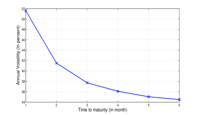
Figure 1: Volatility of electricity Month-ahead futures prices w.r.t. to the time to maturity estimated on the French Power market in 2007.

Hence, a challenge is to be able to describe with a single model, both the non-Gaussianity on the short term and the volatility term structure of the forward curve. One reasonable attempt to do so is to consider the exponential Lévy factor model, proposed in [9] or [12]. The forward price given at time $t$ for delivery at time $T_{d}\geq t$, denoted $F_{t}^{T_{d}}$ is then modeled by a $p$-factors model, such that

$$F_{t}^{T_{d}}=F_{0}^{T_{d}}\exp(m_{t}^{T_{d}}+\sum_{k=1}^{p}X_{t}^{k,{T_{d}}})\ ,\quad\textrm{for all}\ t\in[0,{T_{d}}]\ ,\textrm{where}$$ (6.10)

• $(m_{t}^{T_{d}})_{0\leq t\leq{T_{d}}}$ is a real deterministic trend;

• for any $k=1,\cdots p$, $(X_{t}^{k,{T_{d}}})_{0\leq t\leq{T_{d}}}$ is such that $X_{t}^{k,{T_{d}}}=\int_{0}^{t}\sigma_{k}e^{-\lambda_{k}({T_{d}}-s)}d\Lambda^{k}_{s}$, where $\Lambda=(\Lambda^{1},\cdots,\Lambda^{p})$ is a Lévy process on $\mathbb{R}^{d}$, with $\mathbb{E}[\Lambda^{k}_{1}]=0$ and $Var[\Lambda^{k}_{1}]=1$;

• $\sigma_{k}>0\,,\,\lambda_{k}\geq 0\ ,$ are called respectively the volatilities and the mean-reverting rates.

Hence, forward prices are given as exponentials of additive processes with non-stationary increments. In practice, we consider the case of a one or a two factors model ($p=1$ or $2$), where the first factor $X^{1}$ is a non-Gaussian additive process and the second factor $X^{2}$ is a Brownian motion with $\sigma_{1}\gg\sigma_{2}$. Notice that this kind of model was originally developed and studied in details for interest rates in [32], as an extension of the Heath-Jarrow-Morton model where the Brownian motion has been replaced by a general Lévy process.
Of course, this modeling procedure (6.10), implies incompleteness of the market. Hence, if we aim at pricing and hedging a European call on a forward with maturity $T\leq T_{d}$, it won’t be possible, in general, to hedge perfectly the payoff $(F^{T_{d}}_{T}-K)_{+}$ with a hedging portfolio of forward contracts. Then, a natural approach could consist in looking for the variance optimal initial capital and hedging portfolio. In this framework, the results of Section 3 generalizing the results of Hubalek & al in [24] to the case of non stationary additive process can be useful.

6.3 The non Gaussian two factors model

To simplify let us forget the superscript $T_{d}$ denoting the delivery period (since we will consider a fixed delivery period). We suppose that the forward price $F$ follows the two factors model

$$F_{t}=F_{0}\exp(m_{t}+X^{1}_{t}+X^{2}_{t})\ ,\quad\textrm{for all}\ t\in[0,T_{d}]\ ,\textrm{where}$$ (6.11)

• $m$ is a real deterministic trend starting at $0$. It is supposed to be absolutely continuous w.r.t. Lebesgue;

• $X^{1}_{t}=\int_{0}^{t}\sigma_{s}e^{-\lambda(T_{d}-u)}d\Lambda_{u}$, where $\Lambda$ is a Lévy process on $\mathbb{R}$ with $\Lambda$ following a Normal Inverse Gaussian (NIG) distribution or a Variance Gamma (VG) distribution. Moreover, we will assume that $\mathbb{E}[\Lambda_{1}]=0$ and $Var[\Lambda_{1}]=1$;

• $X^{2}=\sigma_{l}W$ where $W$ is a standard Brownian motion on $\mathbb{R}$;

• $\Lambda$ and $W$ are independent;

• $\sigma_{s}$ and $\sigma_{l}$ standing respectively for the short-term volatility and long-term volatility.

6.4 Verification of the assumptions

The result below helps to extend Theorem 4.1 to the case where $X$ is a finite sum of independent semimartingale additive processes, each one verifying Assumptions 1, 2 and 3 for a given payoff $H=f(s_{0}e^{X_{T}})$.

Lemma 6.1.

Let $X^{1},X^{2}$ be two independent semimartingale additive processes with cumulant generating functions $\kappa^{i}$ and related domains $D^{i},{\cal D}^{i},i=1,2$ characterized in Remark 2.10 and (3.12). Let $f:\mathbb{C}\rightarrow\mathbb{C}$ of the form (3.27).
For $X=X^{1}+X^{2}$ with related domains $D,{\cal D}$ and cumulant generating function $\kappa$, we have the following.

1. $D=D^{1}\cap D^{2}$.

2. ${\cal D}^{1}\cap{\cal D}^{2}\subset{\cal D}$.

3. If $X^{1},X^{2}$ verify Assumptions 1, 2 and 3, then $X$ has the same property.

Proof.

Since $X^{1},X^{2}$ are independent and taking into account Remark 2.10 we obtain 1. and $\kappa_{t}(z)=\kappa_{t}^{1}(z)+\kappa^{2}(z),\ \forall z\in D.$ We denote by $\rho^{i},i=1,2$, the reference variance measures defined in Remark 3.12. Clearly $\rho=\rho^{1}+\rho^{2}$ and $d\rho^{i}\ll d\rho$ with $\|\frac{d\rho^{i}}{d\rho}\|_{\infty}\leq 1$.
If $z\in{\cal D}^{1}\cap{\cal D}^{2}$, we can write

$$\int_{0}^{T}\left|\frac{d\kappa_{t}(z)}{d\rho_{t}}\right|^{2}d\rho_{t} \leq 2\int_{0}^{T}\left|\frac{d\kappa^{1}_{t}(z)}{d\rho^{1}_{t}}\frac{d\rho^{1}_{t}}{d\rho_{t}}\right|^{2}d\rho_{t}+2\int_{0}^{T}\left|\frac{d\kappa^{2}_{t}(z)}{d\rho^{2}_{t}}\frac{d\rho^{2}_{t}}{d\rho_{t}}\right|^{2}d\rho_{t}$$

$$= 2\int_{0}^{T}\left|\frac{d\kappa^{1}_{t}(z)}{d\rho^{1}_{t}}\right|^{2}\frac{d\rho^{1}_{t}}{d\rho_{t}}d\rho^{1}_{t}+2\int_{0}^{T}\left|\frac{d\kappa^{2}_{t}(z)}{d\rho^{2}_{t}}\right|^{2}\frac{d\rho^{2}_{t}}{d\rho_{t}}d\rho^{2}_{t}$$

$$\leq 2\left(\int_{0}^{T}\left|\frac{d\kappa^{1}_{t}(z)}{d\rho^{1}_{t}}\right|^{2}d\rho^{1}_{t}+\int_{0}^{T}\left|\frac{d\kappa^{2}_{t}(z)}{d\rho^{2}_{t}}\right|^{2}d\rho^{2}_{t}\right)\ .$$

This concludes the proof of ${\cal D}^{1}\cap{\cal D}^{2}\subset{\cal D}$ and therefore of the of Point 2.
Finally Point 3. follows then by inspection. ∎

With the two factors model, the forward price $F$ is then given as the exponential of an additive process, $X$, such that for all $t\in[0,{T_{d}}]$,

$$X_{t}=m_{t}+X^{1}_{t}+X^{2}_{t}=m_{t}+\sigma_{s}\int_{0}^{t}e^{-\lambda({T_{d}}-u)}d\Lambda_{u}+\sigma_{l}W_{t}\ .$$ (6.12)

For this model, we formulate the following assumption.

Assumption 5.

1. $2\sigma_{s}\in D_{\Lambda}$.

2. If $\sigma_{l}=0$, we require $\Lambda$ not to have deterministic increments.

3. $f:\mathbb{C}\rightarrow\mathbb{C}$ is of the type (3.27) fulfilling (5.9).

Proposition 6.2.

1. The cumulant generating function of $X$ defined by (6.12), $\kappa:[0,{T_{d}}]\times D\rightarrow\mathbb{C}$ is such that for all $z\in D_{\Lambda}(\sigma_{s})$ and for all $t\in[0,T_{d}]$,

   $$\kappa_{t}(z)=zm_{t}+\frac{z^{2}\sigma^{2}_{l}t}{2}+\int_{0}^{t}\kappa^{\Lambda}(z\sigma_{s}e^{-\lambda({T_{d}}-u)})du\ .$$ (6.13)

   In particular for fixed $z\in D_{\Lambda}(\sigma_{s})$, $t\mapsto\kappa_{t}(z)$ is absolutely continuous w.r.t. Lebesgue measure.

2. Under Assumption 5, Assumptions 1,  2 and 3 are fulfilled.

Proof.

We set $\tilde{X}^{2}=m+X^{2}$. We observe that $D^{2}={\cal D}^{2}=\mathbb{C},\quad\kappa^{2}_{t}(z)=\exp(zm_{t}+z^{2}\sigma_{l}^{2}\frac{t}{2}).$ We recall that $\Lambda$ and $W$ are independent so that $\tilde{X}^{2}$ and $X^{1}$ are independent. For clarity, we only write the proof under the hypothesis that $\Lambda$ has no deterministic increments, the general case could be easily adapted. $X^{1}$ is a process of the type studied at Section 5.1; it verifies Assumption 4 and $D_{\Lambda}(l)$ contains $D_{\Lambda}(\sigma_{s})$.

According to Proposition 5.4, Remark 5.5 and (5.9) it follows that Assumptions 1, 2 and 3 are verified for $X^{1}$. Both statements 1. and 2. are now a consequence of Lemma 6.1. ∎

The solution to the mean-variance problem is provided by Theorem 4.1.

Theorem 6.3.

We suppose Assumption 5. The variance-optimal capital $V_{0}$ and the variance-optimal hedging strategy $\varphi$, solution of the minimization problem $(\ref{problem2})$, are given by Theorem 4.1 and Theorem 3.30, Proposition 3.25 together with the expressions given below:

$$\widetilde{l}_{t}: = \sigma_{s}e^{-\lambda({T_{d}}-t)},$$

$$\gamma(z,t): = \frac{z\sigma^{2}_{l}+\kappa^{\Lambda}((z+1)\widetilde{l}_{t})-\kappa^{\Lambda}(z\widetilde{l}_{t})-\kappa^{\Lambda}(\widetilde{l})_{t}}{\sigma^{2}_{l}+\kappa^{\Lambda}(2\widetilde{l}_{t})-2\kappa^{\Lambda}(\widetilde{l}_{t})},$$

$$\eta(z,t): = \left[zm_{t}+\frac{z^{2}\sigma^{2}_{l}}{2}+\kappa^{\Lambda}(z\widetilde{l}_{t})-\gamma(z,t)\big{(}m_{t}+\frac{\sigma^{2}_{l}}{2}+\kappa^{\Lambda}(\widetilde{l}_{t})\big{)}\right]\,dt\ ,$$

$$\lambda_{t} = \frac{m_{t}+\frac{\sigma_{l}^{2}}{2}+\kappa^{\Lambda}(\widetilde{l}_{t})}{\sigma^{2}_{l}+\kappa^{\Lambda}(2\widetilde{l}_{t})-2\kappa^{\Lambda}(\widetilde{l}_{t})}.$$

Remark 6.4.

Previous formulae are practically exploitable numerically. The last condition to be checked is

$$2\sigma_{s}\in D_{\Lambda}.$$ (6.14)

1. $\Lambda_{1}$ is a Normal Inverse Gaussian random variable; if $\sigma_{s}\leq\frac{\alpha-\beta}{2}$ then $(\ref{E731})$ is verified.

2. $\Lambda_{1}$ is a Variance Gamma random variable then $(\ref{E731})$ is verified; if for instance $\sigma_{s}<\frac{-\beta+\sqrt{\beta^{2}+2\alpha}}{2}\ .$

7 Simulations

We are interested in comparing, in simulations, the Variance Optimal (VO) strategy to the Black-Scholes (BS) strategy when hedging a European call, with payoff $(S_{T}-K)_{+}$, on an underlying stock with log-prices $X_{t}=\log(S_{t})$ that have independent but non Gaussian increments. More precisely, we assume that the underlying is an electricity forward contract $S_{t}=S^{0,T_{d}}_{t}=e^{-r(T_{d}-t)}(F_{t}^{T_{d}}-F_{0}^{T_{d}})$ with delivery date $T_{d}$ equal to the maturity of the call $T_{d}=T$.
First, we consider the case where the log-price process $X$ is an exponential of a Lévy process, continuing the analysis of [24], then we consider the non stationary case. We make use of different simulated data according to the underlying model, stationary in one case, non stationary in the second one.

Our simulations investigate two features which were not considered in [24] (even in the stationary case): first the robustness of the BS hedging strategy w.r.t. the underlying price model, second the sensitivity of the continuous VO strategy w.r.t. to the discreteness of the trading dates.
The VO strategy knows the real incomplete price model (with the real values of parameters) whereas the BS strategy assumes (wrongly) a log-normal price model (with the real values of mean and variance). Of course, the VO strategy is by definition optimal, w.r.t. the quadratic norm. However, both strategies (VO and BS) are implemented in discrete time, hence our goal is precisely to analyze the hedging error outside of the theoretical framework of a continuously rebalanced portfolio. Moreover, we are interested in interpreting quantitatively the differences between both strategies w.r.t. to some characteristics such as the underlying log-returns distribution or the number of trading dates.
The time unit is the year and the interest rate is zero in all our simulations. The initial value of the underlying is $s_{0}=100$ Euros. The maturity of the option is $T=0.25$ i.e. three months from now.

7.1 Exponential Lévy

In this subsection, we simulate the log-price process $X$ as a NIG Lévy process with $X_{1}\,\sim\,NIG(\alpha,\beta,\delta,\mu)$. Five different sets of parameters for the NIG distribution have been considered, going from the case of almost Gaussian returns corresponding to standard equities, to the case of highly non Gaussian returns. The standard set of parameters is estimated on the Month-ahead base forward prices of the French Power market in 2007:

$$\alpha=38.46\,,\ \beta=-3.85\,,\ \delta=6.40\,,\ \mu=0.64\ .$$ (7.15)

Those parameters imply a zero mean, a standard deviation of $41\%$, a skewness (measuring the asymmetry) of $-0.02$ and an excess kurtosis (measuring the fatness of the tails) of $0.01$. The other sets of parameters are obtained by multiplying the parameter $\alpha$ by a coefficient $C$, ($\beta,\delta,\mu$) being such that the first three moments are unchanged. Note that when $C$ grows to infinity the tails of the NIG distribution get closer to the tails of the Gaussian distribution. For instance, Table 1 shows how the excess kurtosis (which is zero for a Gaussian distribution) is modified with the five values of $C$ chosen in our simulations.

Coefficient	$C=0.08$	$C=0.14$	$C=0.2$	$C=1$	$C=2$
$\alpha$	$3.08$	$5.38$	$7.69$	$38.46$	$76.92$
Excess kurtosis	$1.87$	$0.61$	$0.30$	$0.01$	$4.\,10^{-3}$

Table 1: Excess kurtosis of $X_{1}$ for different values of $\alpha$, $(\beta,\delta,\mu)$ insuring the same three first moments.

7.1.1 Strike impact on the initial capital and the hedging ratio

Figure 2 shows the initial capital (on the left graph) and the initial hedge ratio (on the right graph) produced by the VO and the BS strategies as functions of the strike, for three different sets of parameters $C=0.08\,,\ C=1\,,\ C=2$. We consider $N=12$ trading dates, which corresponds to operational practices on electricity markets, for an option expiring in three months. One can observe that BS results are very similar to VO results for $C\geq 1$ i.e. for almost Gaussian returns. However, for small values of $C$, for $C=0.08$, corresponding to highly non Gaussian returns, BS approach under-estimates out-of-the-money options and over-estimates at-the-money options (for $K=99$ Euros the BS initial capital is equal to $8.65$ Euros i.e. $122\%$ of the VO initial capital, while for $K=150$, it vanishes to $23$ Cents i.e. only $57\%$ of the VO initial capital).

   

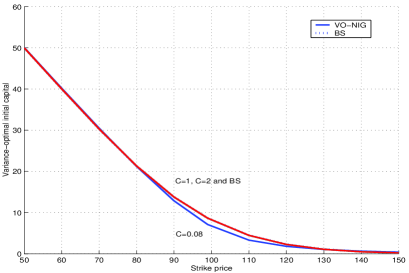
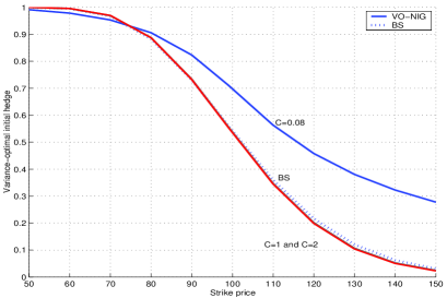
Figure 2: Initial capital (on the left) and hedge ratio (on the right) w.r.t. the strike, for $C=0.08\,,\ C=1\,,\ C=2$.

7.1.2 Hedging error and number of trading dates

Figure 3 considers the hedging error (the difference between the terminal value of the hedging portfolio and the payoff) w.r.t. the number of trading dates, for a strike $K=99$ Euros (at the money) and for five different sets of parameters $C$ given on Table 1. The bias (on the left graph) and standard deviation (on the right graph) of the hedging error have been estimated by Monte Carlo method on $5000$ runs. Note that we could have used the formula stated in Theorem 4.3 to compute the variance of the error, but this would have given us the limiting error which does not take into account the additional error due to the finite number of trading dates.

In terms of standard deviation, the VO strategy seems to outperform noticeably the BS strategy, for small values of $C$ ( for $C=0.08$ the VO strategy allows to reduce $10\%$ of the standard deviation of the error). As expected, one can observe that the VO error converges to the BS error when $C$ increases. This is due to the convergence of NIG log-returns to Gaussian log-returns when $C$ increases (recall that the simulated log-returns are almost symmetric). On Figure 3, the hedging error (both for BS and VO) decreases with the number of trading dates and seems to converge to a limiting error. Here, it is interesting to distinguish two sources of incompleteness, the rebalancing error due to the finite number of trading dates and the intrinsic error due to the price model incompleteness. For instance, one can observe that for small values of $C\leq 0.2$, even for small numbers of trading dates, the intrinsic error seems to be predominant so that it seems useless to increase the number of trading dates over $N\geq 12$ trading dates. Moreover, surprisingly one can observe that for a small number of trading dates $N\leq 12$ and for large values of $C\geq 1$, BS seems to outperform the VO strategy, in terms of standard deviation. This can be interpreted as a consequence of the central limit theorem. Indeed, when the time between two trading dates increases the corresponding increments of the Lévy process converge to a Gaussian variable. Similarly to the observation of [16], section 5., in term of hedging errors, BS strategy seems to be quite close to VO strategy. The same kind of conclusions were obtained in the discrete time setting by [1].

In term of bias, the over-estimation of at-the-money options (observed for $C=0.08$, on Figures 2) seems to induce a positive bias for the BS error (see Figure 3), whereas the bias of the VO error is negligible (as expected from the theory).

   

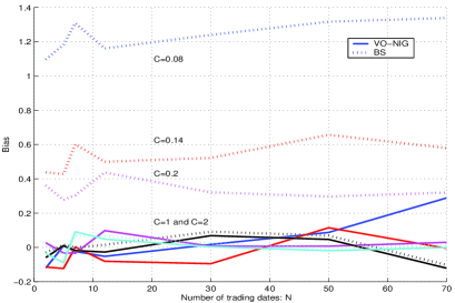
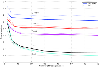
Figure 3: Hedging error w.r.t. the number of trading dates for different values of $C$ and for $K=99$ Euros (bias, on the left and standard deviation, on the right).

7.2 Exponential of additive processes

In this subsection, we simulate the log-price process $X$ as an additive process such that

$$X_{t}=\int_{0}^{t}\sigma_{s}e^{-\lambda(T-u)}d\Lambda_{u}\quad\textrm{where $\Lambda$ is a L\'{e}vy process with }\quad\Lambda_{1}\,\sim\,NIG(\alpha,\beta,\delta,\mu)\ .$$

The standard set of parameters $(C=1)$ for the distribution of $\Lambda_{1}$ is estimated on the same data as in the previous section (Month-ahead base forward prices of the French Power market in 2007):

$$\alpha=15.81\,,\ \beta=-1.581\,,\ \delta=15.57\,,\ \mu=1.56\ .$$

Those parameters correspond to a standard and centered NIG distribution with a skewness of $-0.019$. The estimated annual short-term volatility and mean-reverting rate are $\sigma_{s}=57.47\%$ and $\lambda=3$. The other sets of parameters considered in simulations are obtained by multiplying parameter $\alpha$ by a coefficient $C$, ($\beta,\delta,\mu$ being such that the first three moments are unchanged).

The results are comparable to those obtained in the case of the Lévy process, on Figure 4.

   

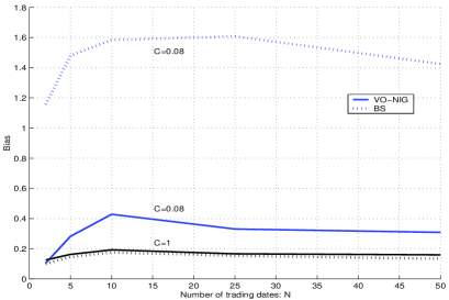
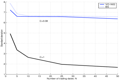
Figure 4: Hedging error w.r.t. the number of trading dates for $C=0.08$ and $C=1$, for $K=99$ Euros (bias, on the left and standard deviation, on the right).

ACKNOWLEDGEMENTS: The first named author was partially founded by Banca Intesa San Paolo. The research of the third named author was partially supported by the ANR Project MASTERIE 2010 BLANC-0121-01. All the authors are grateful to F. Hubalek for useful advices to improve the numerical computations of Laplace transforms performed in simulations. They also thank the Referee for reading carefully the manuscript and making useful comments.

References

- [1] Angelini, F. and Herzel., S. (2009). Measuring the error of dynamic hedging: a Laplace transform approach. Computational Finance, Vol. 12 (2).
- [2] Ansel, J-P. and Stricker, C. (1992). Lois de martingale, densités et décomposition de Föllmer-Schweizer. Annales de l’Institut Henri Poincaré 28, 375-392.
- [3] Arai, T. (2005). Some properties of the variance-optimal martingale measure for discontinuous semimartingales. Statistics and Probability Letters 74, 163-170.
- [4] Arai, T. (2005). An extension of mean-variance hedging to the discontinuous case. Finance and Stochastics 9, 129-139.
- [5] Barndorff-Nielsen, O.E. and Halgreen, C. (1977). Infinite divisibility of the hyperbolic and generalized inverse Gaussian distributions. Zeitschrift für Wahrscheinlichkeitstheorie und verwandte Gebiete, Vol. 38, 309-312.
- [6] Barndorff-Nielsen, O.E. (1998). Processes of normal inverse Gaussian type. Finance and Stochastics 2, 41-68.
- [7] Benth, F. E., Di Nunno, G., Løkka, A., Øksendal, B., Proske, F. (2003). Explicit representation of the minimal variance portfolio in markets driven by Lévy processes. Conference on Applications of Malliavin Calculus in Finance (Rocquencourt, 2001). Math. Finance 13, no. 1, 55–72.
- [8] Benth, F. E. and Saltyte-Benth, J. and Koekebakker, S. (2008). Stochastic modelling of electricity and related markets. Advanced Series on statistical Science & Applied Probability, Vol. 11 / World Scientific.
- [9] Benth, F.E. and Saltyte-Benth, J. (2004). The normal inverse Gaussian distribution and spot price modeling in energy markets. International journal of theoretical and applied finance, Vol. 7(2), 177-192.
- [10] Calvet, L. and Fisher, A. and Mandelbrot, B. (1997). A multifractal model of asset returns. Discussion Papers, Cowles Foundation Yale University: 1164–1166.
- [11] ern, A. and Kallsen, J. (2007). On the structure of general man-variance hedging strategies. The Annals of probability, vol 35 No. 4, 1479-1531.
- [12] Collet, J., Duwig, D. and Oudjane N. (2006). Some non-Gaussian models for electricity spot prices. In Proceedings of the 9th International Conference on Probabilistic Methods Applied to Power Systems.
- [13] Cont, R. and Tankov, P. (2003). Financial modelling with jump processes. Chapman & Hall/CRC Press.
- [14] Cont, R., Tankov, P. and Voltchkova, E. (2007). Hedging with options in models with jumps. Stochastic analysis and applications, 197–217, Abel Symp., 2, Springer, Berlin.
- [15] Cramer, H. (1939). On the representation of a function by certain Fourier integrals. Transactions of the American Mathematical Society 46, 191-201.
- [16] Denkl, S., Goy, M., Kallsen J., Muhle-Karbe, J. and Pauwels, A. (2011). On the Performance of Delta Hedging Strategies in Exponential Lévy Models. Preprint arXiv:0911.4859v3.
- [17] Eberlein, E., Glau, C. and Papapantoleon, A. (2010). Analysis of Fourier transform valuation formula and applications. Appl. Math. Finance, 17, no. 3, 211–240.
- [18] El Karoui, N. and Quenez, M. (1995). Dynamic programming and pricing of contingent claims in an incomplete market. SIAM journal on Control and Optimization, vol 33, 29-66.
- [19] Filipović, D. (2005). Time-inhomogeneous affine processes. Stochastic Processes and Their Applications 115, 639-659.
- [20] Föllmer, H. and Leukert, P. (1999). Quantile hedging. Finance and Stochastics 3, no. 3, 251-273.
- [21] Föllmer, H. and Schweizer, M. (1991). Hedging of contingent claims under incomplete information. M. H. A. Davis and R. J. Elliott (eds.), Applied stochastic analysis, 389-414, Stochastics Monogr., 5, Gordon & Breach, New York.
- [22] Goutte, S., Oudjane, N. and Russo, F. (2010). Variance Optimal Hedging for discrete time processes with independent increments. Application to Electricity Markets. Preprint HAL-INRIA http://hal.inria.fr/inria-00473032 to appear in the Journal of computational Finance in 2013.
- [23] Hodges, S. and Neuberger, A. (1989). Optimal replication of contingent claims under transactions costs. Review of forward markets, vol 8, 222-239.
- [24] Hubalek, F., Kallsen, J. and Krawczyk, L.(2006). Variance-optimal hedging for processes with stationary independent increments. The Annals of Applied Probability, Volume 16, Number 2, 853-885.
- [25] Jacod, J. and Shiryaev, A. (2003). Limit theorems for stochastic processes. 2nd edition. Berlin Springer.
- [26] Kluge, W. (2005). Time-inhomogeneous Lévy processes in interest rate and credit risk modeling. Dissertation, Freiburg. http://www.freidok.uni-freiburg.de/volltexte/2090/pdf/diss.pdf
- [27] Madan, D.B., Carr, P.P. and Chang, E.C. (1998). The variance gamma process and option pricing. European Finance Review, 2, 79-105.
- [28] Mandelbrot, B. B. (1972). Possible Refinements of the Lognormal Hypothesis Concerning the Distribution of Energy Dissipation in Intermittent Turbulence. In: M. Rosenblatt and C. Van Atta eds., Statistical Models and Turbulence, New York: Springer Verlag.
- [29] Meyer-Brandis, T. and Tankov, P. (2008). Multi-factor jump-diffusion models of electricity prices. International Journal of Theoretical and Applied Finance, Vol. 11, No. 5, 503 - 528.
- [30] Monat, P. and Stricker, C. (1995). Föllmer-Schweizer decomposition and mean-variance hedging for general claims. The Annals of Probability, Vol. 23, No.2, 605-628.
- [31] Protter, P. (2004). Stochastic integration and differential equations. 2nd edition. Berlin Springer-Verlag.
- [32] Raible, S. (2000). Lévy processes in finance: theory, numerics and empirical facts. PhD thesis, Freiburg University.
- [33] Rudin, W. (1987). Real and complex analysis. Third edition. New York: McGraw-Hill.
- [34] Samuelson, P.A., (1965). Proof that properly anticipated prices fluctuate randomly. Industrial Management Review 6: 41-49.
- [35] Sato, K. (1999). Lévy processes and infinitely divisible distributions. Cambridge: Cambridge University Press.
- [36] Schäl, M. (1994). On quadratic cost criteria for options hedging. Mathematics of Operations Research 19, 121-131.
- [37] Schwartz, E.S. (1997). The stochastic behaviour of commodity prices: implications for valuation and hedging. Journal of Finance, LII, 923-973.
- [38] Schweizer, M. (1994). Approximating random variables by stochastic integrals. The Annals of Probability Vol. 22, 1536-1575.
- [39] Schweizer, M. (1995). On the minimal martingale measure and the Föllmer-Schweizer decomposition. Stochastic Analysis and Applications, 573-599.
- [40] Schweizer, M. (1995). Variance-optimal hedging in discrete time. Mathematics of Operations Research 20, 1-32.
- [41] Schweizer, M. (1996). Approximation pricing and the variance-optimal martingale measure. The Annals of Probability Vol. 24, 206-236.
- [42] Schweizer, M. (2001). A guided tour through quadratic hedging approaches. Option pricing, interest rates and risk management. 538-574, Handb. Math. Finance, Cambridge Univ. Press, Cambridge.
- [43] Schweizer, M. (2010). Mean variance hedging. In R. Cont (ed.), Encyclopedia of Quantitative Finance, Wiley, 1177-81.