11institutetext: Strategic CAD Labs, Intel 22institutetext: UC Berkeley

SWATI: Synthesizing Wordlengths Automatically Using Testing and Induction

Susmit Jha 1122    Sanjit A. Seshia 22
Abstract

In this paper, we present an automated technique πšœπš πšŠπšπš’πšœπš πšŠπšπš’\mathtt{swati}: Synthesizing Wordlengths Automatically Using Testing and Induction, which uses a combination of Nelder-Mead optimization based testing, and induction from examples to automatically synthesize optimal fixedpoint implementation of numerical routines. The design of numerical software is commonly done using floating-point arithmetic in design-environments such as Matlab. However, these designs are often implemented using fixed-point arithmetic for speed and efficiency reasons especially in embedded systems. The fixed-point implementation reduces implementation cost, provides better performance, and reduces power consumption. The conversion from floating-point designs to fixed-point code is subject to two opposing constraints: (i) the word-width of fixed-point types must be minimized, and (ii) the outputs of the fixed-point program must be accurate. In this paper, we propose a new solution to this problem. Our technique takes the floating-point program, specified accuracy and an implementation cost model and provides the fixed-point program with specified accuracy and optimal implementation cost. We demonstrate the effectiveness of our approach on a set of examples from the domain of automated control, robotics and digital signal processing.

1 Introduction

Numerical software forms a critical component of embedded systems such as robotics, automated control and digital signal processing. These numerical routines have two important characteristics. First, these routines are procedures that compute some mathematical functions designed ignoring precision issues of fixed-point arithmetic. Design environments such as Simulink/Stateflow and LabVIEW allow design and simulation of numerical routines using floating-point arithmetic that closely resembles the more intuitive real arithmetic. Second, the implementation of these numerical routines run in resource-constrained environments, requiring their optimization for low resource cost and high performance. It is common for embedded platforms to have processors without floating-point units due to their added cost and performance penalty. The signal processing/control engineer must thus redesign her floating-point program to instead use fixed-point arithmetic. Each floating-point variable and operation in the original program is simply replaced by a corresponding fixed-point variable and operation, so the basic structure of the program does not change. The tricky part of the redesign process is to find the optimal fixed-point types, viz., the optimal wordlengths (bit-widths) of fixed-point variables, so that the implementation on the platform is optimal β€” lowest cost and highest performance β€” and the resulting fixed-point program is sufficiently accurate. The following novel contributions are made in this paper to address this problem:

  • β€’

    We present a new approach for inductive synthesis of fixed-point programs from floating-point versions. The novelty stems in part from our use of optimization: we not only use optimization routines to minimize fixed-point types (bit-widths of fixed-point variables), as previous approaches have, but also show how to use an optimization oracle to systematically test the program and generate input-output examples for inductive synthesis.

  • β€’

    We illustrate the practical effectiveness of our technique on programs drawn from the domains of digital signal processing and control theory. For the control theory examples, we not only exhibit the synthesized fixed-point programs, but also show that these programs, when integrated in a feedback loop with the rest of the system, perform as accurately as the original floating-point versions.

2 Preliminaries

Floating-point arithmeticΒ [8] is a system for approximately representing real numbers that supports a wide range of values. It approximates a real number using a fixed number of significant digits scaled using an exponent. The floating-point system is so called because the radix point can float anywhere relative to the significant digits of the number. This is in contrast to fixed-point arithmeticΒ [23] in which there are a fixed number of digits and the radix point is also fixed. Due to this feature, a floating-point representation can represent a much wider range of values with the same number of digits. The most common floating-point representation used in computers is that defined by the IEEE 754 StandardΒ [1]. The storage layout of the floating-point numbers consist of three basic components: the sign, the exponent, and the mantissa. The storage layout of the single-precision and double-precision floating point numbers is presented in TableΒ 1

  • β€’

    The sign bit is 00 for a positive number and 111 for a negative number. Flipping the value of this bit flips the sign of the number.

  • β€’

    The mantissa, also known as the significand, represents the precision bits of the number. It is composed of an implicit leading bit and the fraction bits. In order to maximize the quantity of representable numbers, floating-point numbers are typically stored with the radix point after the first non-zero digit. In base 222, the only possible non-zero digit is 111. Thus, we can just assume a leading digit of 1, and don’t need to represent it explicitly. As a result, the mantissa has effectively 242424 bits of resolution, by way of 232323 fraction bits in single-precision floating-point numbers, and 535353 bits of resolution, by way of 525252 fractional bits in double-precision.

  • β€’

    The exponent field needs to represent both positive and negative exponents. To do this, a bias is added to the actual exponent in order to get the stored exponent. For IEEE single-precision floats, this value is 127127127. Thus, an exponent of 00 means that 127127127 is stored in the exponent field. A stored value of 200200200 indicates an exponent of (200βˆ’127)200127(200-127), or 737373. Exponents of βˆ’127127-127 (all 00s) and +128128+128 (all 111s) are reserved for special numbers. For double precision, the exponent field is 111111 bits, and has a bias of 102310231023.

Sign Exponent Fraction Bias
Single Precision 1​[31]1delimited-[]311\;[31] 8​[30βˆ’23]8delimited-[]30238\;[30-23] 23​[22βˆ’00]23delimited-[]220023\;[22-00] 127127127
Double Precision 1​[63]1delimited-[]631\;[63] 11​[62βˆ’52]11delimited-[]625211\;[62-52] 52​[51βˆ’00]52delimited-[]510052\;[51-00] 102310231023
Table 1: Floating-point Number Layout

Floating-point solves a number of representation problems. Fixed-point has a fixed window of representation, which limits it from representing very large or very small numbers. Floating-point, on the other hand, employs a sort of β€œsliding window” of precision appropriate to the scale of the number. The range of positive floating-point numbers can be split into normalized numbers (which preserve the full precision of the mantissa), and denormalized numbers. The denormalized numbers do not have an implicit leading bit of 111 and allow representation of really small numbers but with only a portion of the fraction’s precision. The exponent of all 00s (βˆ’127127-127) and all 111s (128128128) are reserved for denormalized numbers and representing infinity respectively. A complete discussion on the semantics of floating-point operations can be found in the IEEE 754 StandardΒ [1]. A floating-point unit (FPU) is used to carry out operations on floating-point numbers such as addition, subtraction, multiplication, division and square root. FPUs are integrated with CPUs in computers but most embedded processors do not have hardware support for floating-point operations. Emulation of floating-point operations without hardware support can be very slow. Inclusion of FPUs also increases the power consumption of the processors. This has made the use of fixed-point arithmetic very common in embedded systems. In spite of the benefits of floating-point arithmetic, embedded systems often use fixed-point arithmetic to reduce resource cost and improve performance. A fixed-point number consists of a sign mode bit, an integer part and a fractional part. We denote the fixed-point type of a variable xπ‘₯x by πŸπ±β€‹Ο„β€‹(x)𝐟𝐱𝜏π‘₯{\mathbf{fx\tau}}(x). Formally, a fixed-point type is a triple:

βŸ¨πš‚πš’πšπš—πšŽπšπš—πšŽπšœπšœ,π™Έπš†π™»,π™΅πš†π™»βŸ©.πš‚πš’πšπš—πšŽπšπš—πšŽπšœπšœπ™Έπš†π™»π™΅πš†π™»\langle{\mathtt{Signedness}},\mathtt{IWL},\mathtt{FWL}\rangle.

The sign mode bit πš‚πš’πšπš—πšŽπšπš—πšŽπšœπšœπš‚πš’πšπš—πšŽπšπš—πšŽπšœπšœ{\mathtt{Signedness}} is 00 if the data is unsigned and is 111 if the data is signed. The length of the integer part is called the integer wordlength (π™Έπš†π™»π™Έπš†π™»\mathtt{IWL}) and the length of the fractional part is called the fractional wordlength (π™΅πš†π™»π™΅πš†π™»\mathtt{FWL}). The fixed-point wordlength (πš†π™»πš†π™»{\mathtt{WL}}) is the sum of the integer wordlength and fractional wordlength; that is, πš†π™»=π™Έπš†π™»+π™΅πš†π™»πš†π™»π™Έπš†π™»π™΅πš†π™»{\mathtt{WL}}=\mathtt{IWL}+\mathtt{FWL}. A fixed-point number with fractional word length (π™΅πš†π™»π™΅πš†π™»\mathtt{FWL}) is scaled by a factor of 1/2π™΅πš†π™»1superscript2π™΅πš†π™»{1}/{2^{\mathtt{FWL}}}. For example, a fixed point number 011100111001110 with 00 as πš‚πš’πšπš—πšŽπšπš—πšŽπšœπšœπš‚πš’πšπš—πšŽπšπš—πšŽπšœπšœ{\mathtt{Signedness}} , integer wordlength of 3 and fractional wordlength of 2 represents 14Γ—1/22141superscript2214\times{1}/{2^{2}}, that is, 3.53.53.5. Converting a fixed-point number with scaling factor R to another type with scaling factor S, requires multiplying the underlying integer by R and dividing by S; that is, multiplying by the ratio R/S. For example, converting 011100111001110 with 00 as πš‚πš’πšπš—πšŽπšπš—πšŽπšœπšœπš‚πš’πšπš—πšŽπšπš—πšŽπšœπšœ{\mathtt{Signedness}}, integer wordlength of 2 and fractional wordlength of 2 into a fixed-point number with 00 as πš‚πš’πšπš—πšŽπšπš—πšŽπšœπšœπš‚πš’πšπš—πšŽπšπš—πšŽπšœπšœ{\mathtt{Signedness}}, integer wordlength of 2 and fractional wordlength of 3 requires multiplying with 23/22superscript23superscript22{2^{3}}/{2^{2}} to obtain 011100011100011100. If the scaling factor is to be reduced, the new integer will have to be rounded. For example, converting the same fixed-point number 011100111001110 to a fixed-point number with fractional wordlength of 00 and integer wordlength of 222 yields 011011011, that is, 333 which is obtained by rounding down from 3.53.53.5. The operations supported by fixed-point arithmetic are the same as those in the floating-point arithmetic standardΒ [1] but the semantics can differ on custom hardware. For example, the rounding mode for arithmetic operations could be different, and the result could be specified to saturate or overflow/underflow in case the wordlength of a variable is not sufficient to store a computed result. One complete semantics of fixed-point operation is provided with the Fixed-point Toolbox in MatlabΒ [2]. The range of the fixed-point number is much smaller compared to the range of floating-point numbers for the same number of bits since the radix point is fixed and no dynamic adjustment of precision is possible.

Number systems with πš†π™»=32πš†π™»32{\mathtt{WL}}=32 Range Precision
Single-precision Floating-point Β±plus-or-minus\pm 10βˆ’44.85superscript1044.85~{}10^{-44.85} to 1038.53superscript1038.53~{}10^{38.53} Adaptive
Fixed-point type: ⟨1,8,24⟩1824\langle 1,8,24\rangle   βˆ’102.11superscript102.11-10^{2.11} to 102.11superscript102.1110^{2.11} 10βˆ’7.22superscript107.22~{}10^{-7.22}
Fixed-point type: ⟨1,16,16⟩11616\langle 1,16,16\rangle   βˆ’104.52superscript104.52-10^{4.52} to 104.52superscript104.5210^{4.52} 10βˆ’4.82superscript104.82~{}10^{-4.82}
Fixed-point type: ⟨1,24,8⟩1248\langle 1,24,8\rangle   βˆ’106.93superscript106.93-10^{6.93} to 106.93superscript106.9310^{6.93} 10βˆ’2.41superscript102.41~{}10^{-2.41}
Table 2: Range of 323232 bit fixed-point and floating-point numbers

Translating a floating-point program into fixed-point program is non-trivial and requires careful consideration of loss of precision and range. The integer wordlengths and fractional wordlengths of the fixed-point variables need to be carefully selected to ensure that the computation remains accurate to a specified threshold.

3 Problem Definition

We introduce a simple illustrative example to explain the problem of synthesizing an optimal fixed-point program from a floating-point program, and then present the formal problem definition.

3.1 Floating-point Implementation

Given a floating-point program, we need to synthesize fixed-point type for each floating-point variable.

Example 1: The floating-point program in this exampleΒ 1 takes πš›πšŠπšπš’πšžπšœπš›πšŠπšπš’πšžπšœ\mathtt{radius} as the input, and computes the corresponding πšŠπš›πšŽπšŠπšŠπš›πšŽπšŠ\mathtt{area} of the circle. Notice that the fixed-point program is essentially identical to the floating-point version, except that the fixed-point types of variables πš–πš’πš™πš’,πš›πšŠπšπš’πšžπšœ,πšπš–πš’πš™πš’πš›πšŠπšπš’πšžπšœπš\mathtt{mypi,radius,t} and πšŠπš›πšŽπšŠπšŠπš›πšŽπšŠ\mathtt{area} must be identified. Recall that the fixed-point type is a triple βŸ¨πšœπš“,πš’πš πš•πš“,πšπš πš•πš“βŸ©subscriptπšœπš“subscriptπš’πš πš•πš“subscriptπšπš πš•πš“\mathtt{\langle s_{j},iwl_{j},fwl_{j}\rangle} for j𝑗j-th variable where πšœπš“subscriptπšœπš“\mathtt{s_{j}} denotes the πš‚πš’πšπš—πšŽπšπš—πšŽπšœπšœπš‚πš’πšπš—πšŽπšπš—πšŽπšœπšœ{\mathtt{Signedness}} of the variable, πš’πš πš•πš“subscriptπš’πš πš•πš“\mathtt{iwl_{j}} denotes the integer wordlength and πšπš πš•πš“subscriptπšπš πš•πš“\mathtt{fwl_{j}} denotes the fraction wordlength.

Procedure 1 Floating-point program to compute circle area
0:Β Β πš›πšŠπšπš’πšžπšœπš›πšŠπšπš’πšžπšœ\mathtt{radius}
0:Β Β πšŠπš›πšŽπšŠπšŠπš›πšŽπšŠ\mathtt{area}
Β Β double πš–πš’πš™πš’,πš›πšŠπšπš’πšžπšœ,𝚝,πšŠπš›πšŽπšŠπš–πš’πš™πš’πš›πšŠπšπš’πšžπšœπšπšŠπš›πšŽπšŠ\mathtt{mypi,radius,t,area}
Β Β πš–πš’πš™πš’=3.14159265358979323846πš–πš’πš™πš’3.14159265358979323846\mathtt{mypi=3.14159265358979323846}
  𝚝=πš›πšŠπšπš’πšžπšœΓ—πš›πšŠπšπš’πšžπšœπšπš›πšŠπšπš’πšžπšœπš›πšŠπšπš’πšžπšœ\mathtt{t=radius\times radius}
Β Β πšŠπš›πšŽπšŠ=πš–πš’πš™πš’Γ—πšπšŠπš›πšŽπšŠπš–πš’πš™πš’πš\mathtt{area=mypi\times t}
Β Β return Β πšŠπš›πšŽπšŠπšŠπš›πšŽπšŠ\mathtt{area}
Procedure 2 Fixed-point program to compute circle area
0:Β Β πš›πšŠπšπš’πšžπšœπš›πšŠπšπš’πšžπšœ\mathtt{radius}, βŸ¨πšœπš“,πš’πš πš•πš“,πšπš πš•πš“βŸ©subscriptπšœπš“subscriptπš’πš πš•πš“subscriptπšπš πš•πš“\mathtt{\langle s_{j},iwl_{j},fwl_{j}\rangle} for πš“=𝟷,𝟸,𝟹,πŸΊπš“1234\mathtt{j=1,2,3,4}
0:Β Β πšŠπš›πšŽπšŠπšŠπš›πšŽπšŠ\mathtt{area}
Β Β πŸπ±β€‹βŸ¨π¬πŸ,𝐒𝐰π₯𝟏,𝐟𝐰π₯𝟏⟩𝐟𝐱subscript𝐬1subscript𝐒𝐰π₯1subscript𝐟𝐰π₯1\mathbf{fx\langle s_{1},iwl_{1},fwl_{1}\rangle} πš–πš’πš™πš’πš–πš’πš™πš’\mathtt{mypi}
Β Β πŸπ±β€‹βŸ¨π¬πŸ,𝐒𝐰π₯𝟐,𝐟𝐰π₯𝟐⟩𝐟𝐱subscript𝐬2subscript𝐒𝐰π₯2subscript𝐟𝐰π₯2\mathbf{fx\langle s_{2},iwl_{2},fwl_{2}\rangle} πš›πšŠπšπš’πšžπšœπš›πšŠπšπš’πšžπšœ\mathtt{radius}
Β Β πŸπ±β€‹βŸ¨π¬πŸ‘,𝐒𝐰π₯πŸ‘,𝐟𝐰π₯πŸ‘βŸ©πŸπ±subscript𝐬3subscript𝐒𝐰π₯3subscript𝐟𝐰π₯3\mathbf{fx\langle s_{3},iwl_{3},fwl_{3}\rangle} 𝚝𝚝\mathtt{t}
Β Β πŸπ±β€‹βŸ¨π¬πŸ’,𝐒𝐰π₯πŸ’,𝐟𝐰π₯πŸ’βŸ©πŸπ±subscript𝐬4subscript𝐒𝐰π₯4subscript𝐟𝐰π₯4\mathbf{fx\langle s_{4},iwl_{4},fwl_{4}\rangle} πšŠπš›πšŽπšŠπšŠπš›πšŽπšŠ\mathtt{area}
Β Β πš–πš’πš™πš’=3.14159265358979323846πš–πš’πš™πš’3.14159265358979323846\mathtt{mypi=3.14159265358979323846}
  𝚝=πš›πšŠπšπš’πšžπšœΓ—πš›πšŠπšπš’πšžπšœπšπš›πšŠπšπš’πšžπšœπš›πšŠπšπš’πšžπšœ\mathtt{t=radius\times radius}
Β Β πšŠπš›πšŽπšŠ=πš–πš’πš™πš’Γ—πšπšŠπš›πšŽπšŠπš–πš’πš™πš’πš\mathtt{area=mypi\times t}
Β Β return Β πšŠπš›πšŽπšŠπšŠπš›πšŽπšŠ\mathtt{area}

We use Ff​l​(X)subscript𝐹𝑓𝑙𝑋F_{fl}(X) to denote the floating-point program with inputs X=⟨x1,x2,…,xnβŸ©π‘‹subscriptπ‘₯1subscriptπ‘₯2…subscriptπ‘₯𝑛X=\langle x_{1},x_{2},\ldots,x_{n}\rangle. Ff​x​(X,πŸπ±β€‹Ο„)subscript𝐹𝑓π‘₯π‘‹πŸπ±πœF_{fx}(X,{\mathbf{fx\tau}}) denotes the fixed-point version of the program, where the fixed-point type of a variable x∈Xπ‘₯𝑋x\in X is πŸπ±β€‹Ο„β€‹(x)𝐟𝐱𝜏π‘₯{\mathbf{fx\tau}}(x). Note that the fixed-point types in Ff​x​(X,πŸπ±β€‹Ο„)subscript𝐹𝑓π‘₯π‘‹πŸπ±πœF_{fx}(X,{\mathbf{fx\tau}}) are defined by the mapping πŸπ±β€‹Ο„πŸπ±πœ{\mathbf{fx\tau}}.

3.2 Input Domain

The context in which a fixed-point program Ff​x​(X,πŸπ±β€‹Ο„)subscript𝐹𝑓π‘₯π‘‹πŸπ±πœF_{fx}(X,{\mathbf{fx\tau}}) is executed often provides a precondition that must be satisfied by valid inputs ⟨x1,x2,…,xn⟩subscriptπ‘₯1subscriptπ‘₯2…subscriptπ‘₯𝑛\langle x_{1},x_{2},\ldots,x_{n}\rangle. This defines the input domain denoted by D​o​m​(X)π·π‘œπ‘šπ‘‹Dom(X).

Example 2: In our example of computing area of a circle, suppose that we are only interested in the radii in the range [0.1,2.0)0.12.0[0.1,2.0). Then, the input domain D​o​m​(πš›πšŠπšπš’πšžπšœ)π·π‘œπ‘šπš›πšŠπšπš’πšžπšœDom(\mathtt{radius}) is

πš›πšŠπšπš’πšžπšœβ‰₯0.1βˆ§πš›πšŠπšπš’πšžπšœ<2.0πš›πšŠπšπš’πšžπšœ0.1πš›πšŠπšπš’πšžπšœ2.0\mathtt{radius}\geq 0.1\wedge\mathtt{radius}<2.0

3.3 Correctness Condition for Accuracy

The correctness condition specifies an error function E​r​r​(Ff​l​(X),Ff​x​(X,πŸπ±β€‹Ο„))πΈπ‘Ÿπ‘Ÿsubscript𝐹𝑓𝑙𝑋subscript𝐹𝑓π‘₯π‘‹πŸπ±πœErr(F_{fl}(X),F_{fx}(X,{\mathbf{fx\tau}})), and a maximum error threshold πš–πšŠπš‘π™΄πš›πš›πš˜πš›πš–πšŠπš‘π™΄πš›πš›πš˜πš›\mathtt{maxError}. The error function and error threshold together define a bound on the β€œdistance” between outputs generated by the floating-point and fixed-point programs respectively. An accurate fixed-point program is one whose error function lies within the error threshold for all inputs in the input domain. Some common error functions are:

  • βˆ™βˆ™\bullet

    Absolute difference between the floating-point function and fixed-point function: |Ff​l​(X)βˆ’Ff​x​(X,πŸπ±β€‹Ο„)|subscript𝐹𝑓𝑙𝑋subscript𝐹𝑓π‘₯π‘‹πŸπ±πœ\left|F_{fl}(X)-F_{fx}(X,{\mathbf{fx\tau}})\right|

  • βˆ™βˆ™\bullet

    Relative difference between the floating-point function and fixed-point function: |Ff​l​(X)βˆ’Ff​x​(X,πŸπ±β€‹Ο„)Ff​l​(X)|subscript𝐹𝑓𝑙𝑋subscript𝐹𝑓π‘₯π‘‹πŸπ±πœsubscript𝐹𝑓𝑙𝑋\left|\frac{F_{fl}(X)-F_{fx}(X,{\mathbf{fx\tau}})}{F_{fl}(X)}\right|

  • βˆ™βˆ™\bullet

    Moderated relative difference: |Ff​l​(X)βˆ’Ff​x​(X,πŸπ±β€‹Ο„)Ff​l​(X)+Ξ΄|subscript𝐹𝑓𝑙𝑋subscript𝐹𝑓π‘₯π‘‹πŸπ±πœsubscript𝐹𝑓𝑙𝑋𝛿\left|\frac{F_{fl}(X)-F_{fx}(X,{\mathbf{fx\tau}})}{F_{fl}(X)+\delta}\right|. This approaches the relative difference for Ff​l​(X)>>Ξ΄much-greater-thansubscript𝐹𝑓𝑙𝑋𝛿F_{fl}(X)>>\delta and approaches a weighted absolute difference for Ff​l​(X)<<Ξ΄much-less-thansubscript𝐹𝑓𝑙𝑋𝛿F_{fl}(X)<<\delta. When Ff​l​(X)subscript𝐹𝑓𝑙𝑋F_{fl}(X) can be zero for some values of X𝑋X, the moderated relative difference remains bounded unlike the relative difference which becomes unbounded.

The correctness condition for accuracy requires that for all inputs in the provided input domain D​o​m​(X)π·π‘œπ‘šπ‘‹Dom(X), the error function E​r​r​(Ff​l​(X),Ff​x​(X,πŸπ±β€‹Ο„))πΈπ‘Ÿπ‘Ÿsubscript𝐹𝑓𝑙𝑋subscript𝐹𝑓π‘₯π‘‹πŸπ±πœErr(F_{fl}(X),F_{fx}(X,{\mathbf{fx\tau}})) is below the specified threshold πš–πšŠπš‘π™΄πš›πš›πš˜πš›πš–πšŠπš‘π™΄πš›πš›πš˜πš›\mathtt{maxError}; i.e.,

βˆ€X∈D​o​m​(X).E​r​r​(Ff​l​(X),Ff​x​(X,πŸπ±β€‹Ο„))β‰€πš–πšŠπš‘π™΄πš›πš›πš˜πš›formulae-sequencefor-allπ‘‹π·π‘œπ‘šπ‘‹πΈπ‘Ÿπ‘Ÿsubscript𝐹𝑓𝑙𝑋subscript𝐹𝑓π‘₯π‘‹πŸπ±πœπš–πšŠπš‘π™΄πš›πš›πš˜πš›\forall X\in Dom(X)\;.\;Err(F_{fl}(X),F_{fx}(X,{\mathbf{fx\tau}}))\leq\mathtt{maxError}

Example 3: In our running example of computing area of a circle, the error function is chosen to be relative difference, the error threshold 0.010.010.01, and thus the correctness condition is βˆ€πš›πšŠπšπš’πšžπšœ,s.t.πš›πšŠπšπš’πšžπšœβ‰₯0.1βˆ§πš›πšŠπšπš’πšžπšœ<2.0formulae-sequencefor-allπš›πšŠπšπš’πšžπšœπ‘ π‘‘πš›πšŠπšπš’πšžπšœ0.1πš›πšŠπšπš’πšžπšœ2.0\forall\mathtt{radius},\;s.t.\;\mathtt{radius}\geq 0.1\wedge\mathtt{radius}<2.0

Ff​l​(πš›πšŠπšπš’πšžπšœ)βˆ’Ff​x​(πš›πšŠπšπš’πšžπšœ,πŸπ±β€‹Ο„)Ff​l​(πš›πšŠπšπš’πšžπšœ)≀0.01subscriptπΉπ‘“π‘™πš›πšŠπšπš’πšžπšœsubscript𝐹𝑓π‘₯πš›πšŠπšπš’πšžπšœπŸπ±πœsubscriptπΉπ‘“π‘™πš›πšŠπšπš’πšžπšœ0.01\frac{F_{fl}(\mathtt{radius})-F_{fx}(\mathtt{radius},{\mathbf{fx\tau}})}{F_{fl}(\mathtt{radius})}\leq 0.01

3.4 Implementation Cost Model

The cost model of the fixed-point program is a function mapping fixed-point types to a real number. For a given fixed-point program Ff​x​(X,πŸπ±β€‹Ο„)subscript𝐹𝑓π‘₯π‘‹πŸπ±πœF_{fx}(X,{\mathbf{fx\tau}}), let T={t1,t2,…,tk}𝑇subscript𝑑1subscript𝑑2…subscriptπ‘‘π‘˜T=\{t_{1},t_{2},\ldots,t_{k}\} be the set of fixed-point program variables with corresponding types {πŸπ±β€‹Ο„β€‹(t1),πŸπ±β€‹Ο„β€‹(t2),…,πŸπ±β€‹Ο„β€‹(tk)}𝐟𝐱𝜏subscript𝑑1𝐟𝐱𝜏subscript𝑑2β€¦πŸπ±πœsubscriptπ‘‘π‘˜\{{\mathbf{fx\tau}}(t_{1}),{\mathbf{fx\tau}}(t_{2}),\ldots,{\mathbf{fx\tau}}(t_{k})\}. Then the cost model (or simply cost) of Ff​xsubscript𝐹𝑓π‘₯F_{fx} is a function

𝚌𝚘𝚜𝚝:(πŸπ±β€‹Ο„β€‹(t1),πŸπ±β€‹Ο„β€‹(t2),…,πŸπ±β€‹Ο„β€‹(tk))→ℝ:πšŒπš˜πšœπšβ†’πŸπ±πœsubscript𝑑1𝐟𝐱𝜏subscript𝑑2β€¦πŸπ±πœsubscriptπ‘‘π‘˜β„{\mathtt{cost}}:({\mathbf{fx\tau}}(t_{1}),{\mathbf{fx\tau}}(t_{2}),\ldots,{\mathbf{fx\tau}}(t_{k}))\rightarrow\mathbb{R}

In practice, 𝚌𝚘𝚜𝚝𝚌𝚘𝚜𝚝{\mathtt{cost}} is often just a function of the total wordlengths (πš†π™»=π™Έπš†π™»+π™΅πš†π™»πš†π™»π™Έπš†π™»π™΅πš†π™»{\mathtt{WL}}=\mathtt{IWL}+\mathtt{FWL}) of the variables. It can incorporate hardware implementation metrics such as area, power and delay. A number of cost models are available in the literatureΒ [16, 17, 5, 6], and all of these can be used in our approach.
Example 4: The cost model proposed by Constantinides et alΒ [6] for the running example yields the following cost function. We use this cost model in all our examples.

πšŒπš˜πšœπšβ€‹(πŸπ±β€‹Ο„β€‹(πš–πš’πš™πš’),πŸπ±β€‹Ο„β€‹(πš›πšŠπšπš’πšžπšœ),πŸπ±β€‹Ο„β€‹(𝚝),πŸπ±β€‹Ο„β€‹(πšŠπš›πšŽπšŠ))=πšŒπš˜πšœπšπŸπ±πœπš–πš’πš™πš’πŸπ±πœπš›πšŠπšπš’πšžπšœπŸπ±πœπšπŸπ±πœπšŠπš›πšŽπšŠabsent{\mathtt{cost}}({\mathbf{fx\tau}}(\mathtt{mypi}),{\mathbf{fx\tau}}(\mathtt{radius}),{\mathbf{fx\tau}}(\mathtt{t}),{\mathbf{fx\tau}}(\mathtt{area}))=
πšŒπšπšŽπš•πšŠπš’β€‹(πš†π™»β€‹(πš–πš’πš™πš’))+πšŒπš–πšžπš•β€‹(πš†π™»β€‹(πš›πšŠπšπš’πšžπšœ),πš†π™»β€‹(πš›πšŠπšπš’πšžπšœ),πš†π™»β€‹(𝚝))πšŒπšπšŽπš•πšŠπš’πš†π™»πš–πš’πš™πš’πšŒπš–πšžπš•πš†π™»πš›πšŠπšπš’πšžπšœπš†π™»πš›πšŠπšπš’πšžπšœπš†π™»πš{\mathtt{cdelay}}({\mathtt{WL}}(\mathtt{mypi}))+{\mathtt{cmul}}({\mathtt{WL}}(\mathtt{radius}),{\mathtt{WL}}(\mathtt{radius}),{\mathtt{WL}}(\mathtt{t}))
+πšŒπš–πšžπš•β€‹(πš†π™»β€‹(πš–πš’πš™πš’),πš†π™»β€‹(𝚝),πš†π™»β€‹(πšŠπš›πšŽπšŠ)),πš πš‘πšŽπš›πšŽπšŒπš–πšžπš•πš†π™»πš–πš’πš™πš’πš†π™»πšπš†π™»πšŠπš›πšŽπšŠπš πš‘πšŽπš›πšŽ+{\mathtt{cmul}}({\mathtt{WL}}(\mathtt{mypi}),{\mathtt{WL}}(\mathtt{t}),{\mathtt{WL}}(\mathtt{area}))\;,\mathtt{where}
πšŒπšπšŽπš•πšŠπš’β€‹(l)=l+1β€‹πšŠπš—πšβ€‹πšŒπš–πšžπš•β€‹(l1,l2,l)=0.6Γ—(l1+1)βˆ—l2βˆ’0.85βˆ—(l1+l2βˆ’l)πšŒπšπšŽπš•πšŠπš’π‘™π‘™1πšŠπš—πšπšŒπš–πšžπš•subscript𝑙1subscript𝑙2𝑙0.6subscript𝑙11subscript𝑙20.85subscript𝑙1subscript𝑙2𝑙{\mathtt{cdelay}}(l)=l+1\;\mathtt{and}\;{\mathtt{cmul}}(l_{1},l_{2},l)=0.6\times(l_{1}+1)*l_{2}-0.85*(l_{1}+l_{2}-l)

The area of a multiplier grows almost linearly with both the coefficients and the data wordlength. The first term in the Constantinides model represents this cost. The second term represents the area cost of computational elements required only for carry propagation. The coefficients 0.60.60.6 and 0.850.850.85 were obtained through least-squared fitting to area of several hundred multipliers of different coefficient value and widthΒ [6].

3.5 Problem Definition

Definition 1 (Optimal Fixed-point Types Synthesis)

The optimal fixed-point types synthesis problem is as follows. Given a floating-point program Ff​x​(X,πŸπ±β€‹Ο„β€‹(T))subscript𝐹𝑓π‘₯π‘‹πŸπ±πœπ‘‡F_{fx}(X,{\mathbf{fx\tau}}(T)) with variables T𝑇T, an input domain D​o​m​(X)π·π‘œπ‘šπ‘‹Dom(X), a correctness condition E​r​r​(Ff​l​(X),Ff​x​(X,πŸπ±β€‹Ο„β€‹(T)))β‰€πš–πšŠπš‘π™΄πš›πš›πš˜πš›πΈπ‘Ÿπ‘Ÿsubscript𝐹𝑓𝑙𝑋subscript𝐹𝑓π‘₯π‘‹πŸπ±πœπ‘‡πš–πšŠπš‘π™΄πš›πš›πš˜πš›Err(F_{fl}(X),F_{fx}(X,{\mathbf{fx\tau}}(T)))\leq\mathtt{maxError}, and a cost model πšŒπš˜πšœπšβ€‹(πŸπ±β€‹Ο„β€‹(t1),πŸπ±β€‹Ο„β€‹(t2),…,πŸπ±β€‹Ο„β€‹(tk))𝚌𝚘𝚜𝚝𝐟𝐱𝜏subscript𝑑1𝐟𝐱𝜏subscript𝑑2β€¦πŸπ±πœsubscriptπ‘‘π‘˜{\mathtt{cost}}({\mathbf{fx\tau}}(t_{1}),{\mathbf{fx\tau}}(t_{2}),\ldots,{\mathbf{fx\tau}}(t_{k})), the optimal fixed-point types synthesis problem is to discover fixed-point types

πŸπ±β€‹Ο„βˆ—β€‹(T)={πŸπ±β€‹Ο„βˆ—β€‹(t1),πŸπ±β€‹Ο„βˆ—β€‹(t2),…,πŸπ±β€‹Ο„βˆ—β€‹(tk)}𝐟𝐱superscriptπœπ‘‡πŸπ±superscript𝜏subscript𝑑1𝐟𝐱superscript𝜏subscript𝑑2β€¦πŸπ±superscript𝜏subscriptπ‘‘π‘˜{\mathbf{fx\tau}}^{*}(T)=\{{\mathbf{fx\tau}}^{*}(t_{1}),{\mathbf{fx\tau}}^{*}(t_{2}),\ldots,{\mathbf{fx\tau}}^{*}(t_{k})\}

such that the fixed-point program Ff​l​(X)subscript𝐹𝑓𝑙𝑋F_{fl}(X) with the above types for fixed-point variables satisfies the correctness condition for accuracy, that is,

(a)β€‹βˆ€X∈D​o​m​(X).E​r​r​(Ff​l​(X),Ff​x​(X,πŸπ±β€‹Ο„βˆ—β€‹(T)))β‰€πš–πšŠπš‘π™΄πš›πš›πš˜πš›formulae-sequenceπ‘Žfor-allπ‘‹π·π‘œπ‘šπ‘‹πΈπ‘Ÿπ‘Ÿsubscript𝐹𝑓𝑙𝑋subscript𝐹𝑓π‘₯π‘‹πŸπ±superscriptπœπ‘‡πš–πšŠπš‘π™΄πš›πš›πš˜πš›(a)\;\forall X\in Dom(X)\;.\;Err(F_{fl}(X),F_{fx}(X,{\mathbf{fx\tau}}^{*}(T)))\leq\mathtt{maxError}

and has minimal cost with respect to the given cost function among all fixed-point types that satisfy condition (a), that is,

(b)β€‹πŸπ±β€‹Ο„βˆ—=argminπŸπ±β€‹Ο„β€‹πšœπšŠπšπš’πšœπšπš’πšŽπšœβ€‹(𝚊)β€‹πšŒπš˜πšœπšβ€‹(πŸπ±β€‹Ο„β€‹(T))π‘πŸπ±superscriptπœπŸπ±πœπšœπšŠπšπš’πšœπšπš’πšŽπšœπšŠargminπšŒπš˜πšœπšπŸπ±πœπ‘‡(b)\;{\mathbf{fx\tau}}^{*}=\underset{{\mathbf{fx\tau}}\mathtt{\;satisfies\;(a)}}{\operatorname{argmin}}\;{\mathtt{cost}}({\mathbf{fx\tau}}(T))

Our goal is to automated this search for optimal fixed-point types. We illustrate this problem using the running example below.

Example 5: In our running example of computing the area of a circle, we need to discover πŸπ±β€‹Ο„βˆ—β€‹(πš–πš’πš™πš’),𝐟𝐱superscriptπœπš–πš’πš™πš’{\mathbf{fx\tau}}^{*}(\mathtt{mypi}), πŸπ±β€‹Ο„βˆ—β€‹(πš›πšŠπšπš’πšžπšœ),𝐟𝐱superscriptπœπš›πšŠπšπš’πšžπšœ{\mathbf{fx\tau}}^{*}(\mathtt{radius}), πŸπ±β€‹Ο„βˆ—β€‹(𝚝)𝐟𝐱superscript𝜏𝚝{\mathbf{fx\tau}}^{*}(\mathtt{t}) and πŸπ±β€‹Ο„βˆ—β€‹(πšŠπš›πšŽπšŠ)𝐟𝐱superscriptπœπšŠπš›πšŽπšŠ{\mathbf{fx\tau}}^{*}(\mathtt{area}) such that

  1. (a)

    the fixed-point program with the given fixed-point types satisfies the correctness condition; that is, βˆ€πš›πšŠπšπš’πšžπšœ,s.t.,πš›πšŠπšπš’πšžπšœβ‰₯0.1βˆ§πš›πšŠπšπš’πšžπšœ<2.0\forall\mathtt{radius},\;s.t.,\;\mathtt{radius}\geq 0.1\wedge\mathtt{radius}<2.0

    Ff​l​(πš›πšŠπšπš’πšžπšœ)βˆ’Ff​x​(πš›πšŠπšπš’πšžπšœ,πŸπ±β€‹Ο„βˆ—)Ff​l​(πš›πšŠπšπš’πšžπšœ)≀0.01subscriptπΉπ‘“π‘™πš›πšŠπšπš’πšžπšœsubscript𝐹𝑓π‘₯πš›πšŠπšπš’πšžπšœπŸπ±superscript𝜏subscriptπΉπ‘“π‘™πš›πšŠπšπš’πšžπšœ0.01\;\;\frac{F_{fl}(\mathtt{radius})-F_{fx}(\mathtt{radius},{\mathbf{fx\tau}}^{*})}{F_{fl}(\mathtt{radius})}\leq 0.01
  2. (b)

    and the cost is minimized; that is,

    πŸπ±β€‹Ο„βˆ—=argminπŸπ±β€‹Ο„β€‹πšœπšŠπšπš’πšœπšπš’πšŽπšœβ€‹(𝚊)β€‹πšŒπš˜πšœπšβ€‹(πŸπ±β€‹Ο„β€‹(πš–πš’πš™πš’,πš›πšŠπšπš’πšžπšœ,𝚝,πšŠπš›πšŽπšŠ))𝐟𝐱superscriptπœπŸπ±πœπšœπšŠπšπš’πšœπšπš’πšŽπšœπšŠargminπšŒπš˜πšœπšπŸπ±πœπš–πš’πš™πš’πš›πšŠπšπš’πšžπšœπšπšŠπš›πšŽπšŠ\;\;{\mathbf{fx\tau}}^{*}=\underset{{\mathbf{fx\tau}}\mathtt{\;satisfies\;(a)}}{\operatorname{argmin}}\;{\mathtt{cost}}({\mathbf{fx\tau}}(\mathtt{mypi},\mathtt{radius},\mathtt{t},\mathtt{area}))

We use this example to illustrate the trade-off between cost and error and how a human might use trial and error to discover the correct wordlengths. We vary the wordlength of the variables. The integer wordlength is selected to avoid overflow and the remaining bits are used for fractional wordlength.

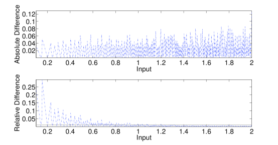
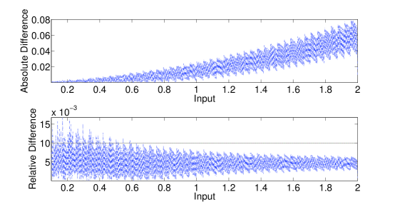
Case 1 (FigureΒ 1): W​L=8π‘ŠπΏ8WL=8 for all variables. πŸπ±β€‹Ο„β€‹(πš–πš’πš™πš’)=⟨0,2,6⟩,πŸπ±β€‹Ο„β€‹(πš›πšŠπšπš’πšžπšœ)=⟨0,1,7⟩,πŸπ±β€‹Ο„β€‹(𝚝)=⟨0,2,6⟩,πŸπ±β€‹Ο„β€‹(πšŠπš›πšŽπšŠ)=⟨0,4,4⟩formulae-sequenceπŸπ±πœπš–πš’πš™πš’026formulae-sequenceπŸπ±πœπš›πšŠπšπš’πšžπšœ017formulae-sequence𝐟𝐱𝜏𝚝026πŸπ±πœπšŠπš›πšŽπšŠ044{\mathbf{fx\tau}}(\mathtt{mypi})=\langle 0,2,6\rangle,{\mathbf{fx\tau}}(\mathtt{radius})=\langle 0,1,7\rangle,{\mathbf{fx\tau}}(\mathtt{t})=\langle 0,2,6\rangle,{\mathbf{fx\tau}}(\mathtt{area})=\langle 0,4,4\rangle. Cost is 81.8081.8081.80.
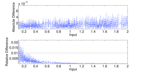
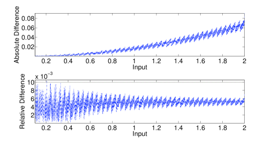
Case 2 (FigureΒ 2): W​L=12π‘ŠπΏ12WL=12 for all variables. πŸπ±β€‹Ο„β€‹(πš–πš’πš™πš’)=⟨0,2,10⟩,πŸπ±β€‹Ο„β€‹(πš›πšŠπšπš’πšžπšœ)=⟨0,1,11⟩,πŸπ±β€‹Ο„β€‹(𝚝)=⟨0,2,10⟩,πŸπ±β€‹Ο„β€‹(πšŠπš›πšŽπšŠ)=⟨0,4,8⟩formulae-sequenceπŸπ±πœπš–πš’πš™πš’0210formulae-sequenceπŸπ±πœπš›πšŠπšπš’πšžπšœ0111formulae-sequence𝐟𝐱𝜏𝚝0210πŸπ±πœπšŠπš›πšŽπšŠ048{\mathbf{fx\tau}}(\mathtt{mypi})=\langle 0,2,10\rangle,{\mathbf{fx\tau}}(\mathtt{radius})=\langle 0,1,11\rangle,{\mathbf{fx\tau}}(\mathtt{t})=\langle 0,2,10\rangle,{\mathbf{fx\tau}}(\mathtt{area})=\langle 0,4,8\rangle. Cost is 179.80179.80179.80.
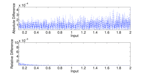
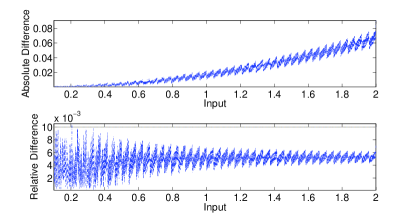
Case 3 (FigureΒ 3): W​L=16π‘ŠπΏ16WL=16 for all variables. πŸπ±β€‹Ο„β€‹(πš–πš’πš™πš’)=⟨0,2,14⟩,πŸπ±β€‹Ο„β€‹(πš›πšŠπšπš’πšžπšœ)=⟨0,1,15⟩,πŸπ±β€‹Ο„β€‹(𝚝)=⟨0,2,14⟩,πŸπ±β€‹Ο„β€‹(πšŠπš›πšŽπšŠ)=⟨0,4,12⟩formulae-sequenceπŸπ±πœπš–πš’πš™πš’0214formulae-sequenceπŸπ±πœπš›πšŠπšπš’πšžπšœ0115formulae-sequence𝐟𝐱𝜏𝚝0214πŸπ±πœπšŠπš›πšŽπšŠ0412{\mathbf{fx\tau}}(\mathtt{mypi})=\langle 0,2,14\rangle,{\mathbf{fx\tau}}(\mathtt{radius})=\langle 0,1,15\rangle,{\mathbf{fx\tau}}(\mathtt{t})=\langle 0,2,14\rangle,{\mathbf{fx\tau}}(\mathtt{area})=\langle 0,4,12\rangle. Cost is 316.20316.20316.20.

Refer to caption
Figure 1: Error for πš†π™»=8πš†π™»8{\mathtt{WL}}=8. Error threshold at 0.010.010.01 is violated.
Refer to caption
Figure 2: πš†π™»=12πš†π™»12{\mathtt{WL}}=12. Error threshold at 0.010.010.01 is violated.
Refer to caption
Figure 3: πš†π™»=16πš†π™»16{\mathtt{WL}}=16. Error threshold at 0.010.010.01 is not violated.

As we will show in the next section, our approach computes fixed-point types that meet the accuracy threshold and yield a cost of only 104.65104.65104.65, which, while being less than the cost in Case 1, satisfies the correctness criterion like Case 2. In the following section, we discuss our automated approach to solve this problem.

4 Our Approach

A central idea behind our approach, πšœπš πšŠπšπš’πšœπš πšŠπšπš’\mathtt{swati} is to identify a small set of interesting inputs S​(X)𝑆𝑋S(X) using testing from the input domain D​o​m​(X)π·π‘œπ‘šπ‘‹Dom(X) such that the optimal implementation found using induction that satisfies the correctness condition for the inputs in S​(X)𝑆𝑋S(X) will be optimal and correct for all inputs in the given input domain D​o​m​(X)π·π‘œπ‘šπ‘‹Dom(X).

Procedure 3 Overall Synthesis Algorithm: πšœπš πšŠπšπš’πšœπš πšŠπšπš’\mathtt{swati}
0:Β Β Floating-point program Ff​psubscript𝐹𝑓𝑝F_{fp},Fixed-point program Ff​xsubscript𝐹𝑓π‘₯F_{fx} with fixed-point variables T𝑇T,Domain of inputs D​o​mπ·π‘œπ‘šDom, Error function E​r​rπΈπ‘Ÿπ‘ŸErr,maximum error threshold πš–πšŠπš‘π™΄πš›πš›πš˜πš›πš–πšŠπš‘π™΄πš›πš›πš˜πš›\mathtt{maxError}, Cost Model 𝚌𝚘𝚜𝚝𝚌𝚘𝚜𝚝{\mathtt{cost}},maximum wordlengths πš†π™»m​a​xsubscriptπš†π™»π‘šπ‘Žπ‘₯{\mathtt{WL}}_{max}
0:Β Β Fixed-point type πŸπ±β€‹Ο„πŸπ±πœ{\mathbf{fx\tau}} for variables T𝑇TΒ Β Β Β Β Β Β Β Β Β  or infeasible
Β Β S0superscript𝑆0S^{0} = random sample from D​o​mπ·π‘œπ‘šDom, B​a​d0=S0π΅π‘Žsuperscript𝑑0superscript𝑆0Bad^{0}=S^{0}, i=0𝑖0i=0
Β Β whileΒ B​a​diβ‰ βˆ…π΅π‘Žsuperscript𝑑𝑖Bad^{i}\not=\emptysetΒ do
Β Β Β Β Β i=i+1𝑖𝑖1i=i+1
Β Β Β Β Β Si=Siβˆ’1βˆͺB​a​diβˆ’1superscript𝑆𝑖superscript𝑆𝑖1π΅π‘Žsuperscript𝑑𝑖1S^{i}=S^{i-1}\cup Bad^{i-1}
Β Β Β Β Β πŸπ±Ο„i=πš˜πš™πšπ™Έπš—πšπšžπšŒπšŽ(Ff​p,Ff​x,Dom,Err,πš–πšŠπš‘π™΄πš›πš›πš˜πš›,{\mathbf{fx\tau}}^{i}=\mathtt{optInduce}{}(F_{fp},F_{fx},Dom,Err,\mathtt{maxError},𝚌𝚘𝚜𝚝,πš†π™»m​a​x,Si)\;\;\;\;\;\;\;\;\;\;\;\;\;\;\;\;\;\;\;\;\;\;\;\;\;\;\;\;\;\;\;\;\;\;\;\;\;\;{\mathtt{cost}},{\mathtt{WL}}_{max},S^{i})
Β Β Β Β Β ifΒ πŸπ±β€‹Ο„i=βŠ₯𝐟𝐱superscriptπœπ‘–bottom{\mathbf{fx\tau}}^{i}=\botΒ then
Β Β Β Β Β Β Β Β return Β infeasible
Β Β Β Β Β endΒ if
Β Β Β Β Β B​a​di=πšπšŽπšœπšπ™΄πš›πš›β€‹(Ff​p,Ff​x,πŸπ±β€‹Ο„i,D​o​m,E​r​r,πš–πšŠπš‘π™΄πš›πš›πš˜πš›)π΅π‘Žsuperscriptπ‘‘π‘–πšπšŽπšœπšπ™΄πš›πš›subscript𝐹𝑓𝑝subscript𝐹𝑓π‘₯𝐟𝐱superscriptπœπ‘–π·π‘œπ‘šπΈπ‘Ÿπ‘Ÿπš–πšŠπš‘π™΄πš›πš›πš˜πš›Bad^{i}=\mathtt{testErr}(F_{fp},F_{fx},{\mathbf{fx\tau}}^{i},Dom,Err,\mathtt{maxError})
Β Β endΒ while
Β Β return Β πŸπ±β€‹Ο„βˆ—=πŸπ±β€‹Ο„i𝐟𝐱superscript𝜏𝐟𝐱superscriptπœπ‘–{\mathbf{fx\tau}}^{*}={\mathbf{fx\tau}}^{i}

The top-level synthesis algorithm is presented in ProcedureΒ 3. πš†π™»m​a​xsubscriptπš†π™»π‘šπ‘Žπ‘₯{\mathtt{WL}}_{max} is an upper bound on wordlengths beyond which it is non-optimal to use the fixed-point version. The algorithm starts with a randomly selected set of examples S0superscript𝑆0S^{0} from the given input domain. Then, a fixed-point implementation that satisfies the accuracy condition for each of these inputs and is of minimal cost is synthesized using the routine πš˜πš™πšπ™Έπš—πšπšžπšŒπšŽπš˜πš™πšπ™Έπš—πšπšžπšŒπšŽ\mathtt{optInduce}. If no such implementation is found, the algorithm reports infeasible. Otherwise, the testing routine πšπšŽπšœπšπ™΄πš›πš›πšπšŽπšœπšπ™΄πš›πš›\mathtt{testErr} checks whether the implementation fails the correctness condition for any input. If so, a set of inputs B​a​diπ΅π‘Žsuperscript𝑑𝑖Bad^{i} on which the implementation violates the correctness condition are added to the set Sisuperscript𝑆𝑖S^{i} used for synthesis, and the process is repeated. If the correctness condition is satisfied, the resulting fixed-point types are output. In the rest of this section, we describe the main components of our approach in detail, including the theoretical result.

4.1 Synthesizing Optimal Types for a Finite Input Set

The πš˜πš™πšπ™Έπš—πšπšžπšŒπšŽπš˜πš™πšπ™Έπš—πšπšžπšŒπšŽ\mathtt{optInduce} function (see ProcedureΒ 4) is used to obtain optimum fixed-point types such that the fixed-point program with these types satisfies the correctness condition for a finite input set S𝑆S and has minimal cost. First, the floating-point program Ff​lsubscript𝐹𝑓𝑙F_{fl} is executed for all the inputs in the sample S𝑆S and the range of each variable tisubscript𝑑𝑖t_{i} as well as its πš‚πš’πšπš—πšŽπšπš—πšŽπšœπšœπš‚πš’πšπš—πšŽπšπš—πšŽπšœπšœ{\mathtt{Signedness}} is recorded by the functions πšπšŽπšπšπšŠπš—πšπšŽπšπšŽπšπšπšŠπš—πšπšŽ\mathtt{getRange} and πš’πšœπš‚πš’πšπš—πšŽπšπš’πšœπš‚πš’πšπš—πšŽπš\mathtt{isSigned} respectively. Then, the integer wordlength π™Έπš†π™»π™Έπš†π™»\mathtt{IWL} sufficient to represent the computed range is assigned to each variable tisubscript𝑑𝑖t_{i} and the πš‚πš’πšπš—πšŽπšπš—πšŽπšœπšœπš‚πš’πšπš—πšŽπšπš—πšŽπšœπšœ{\mathtt{Signedness}} is 111 if the variable takes both positive and negative values, and 00 otherwise. If the fixed-point program with maximum wordlengths πš†π™»m​a​xsubscriptπš†π™»π‘šπ‘Žπ‘₯{\mathtt{WL}}_{max} fails the correctness condition, we conclude that the synthesis is not feasible and return βŠ₯bottom\bot. If not, we search for the wordlength with minimum cost satisfying the correctness condition using our optimization oracle π’ͺSsubscriptπ’ͺ𝑆{\mathcal{O}}_{S}. The result is used to compute the fractional wordlengths, and the resulting fixed-point types are returned.

More precisely, π’ͺSsubscriptπ’ͺ𝑆{\mathcal{O}}_{S} solves the following optimization problem over πŸπ±β€‹Ο„πŸπ±πœ{\mathbf{fx\tau}}: π™Όπš’πš—πš’πš–πš’πš£πšŽβ€‹πšŒπš˜πšœπšβ€‹(πŸπ±β€‹Ο„)β€‹πšœ.𝚝.formulae-sequenceπ™Όπš’πš—πš’πš–πš’πš£πšŽπšŒπš˜πšœπšπŸπ±πœπšœπš\mathtt{Minimize\;\;}{\mathtt{cost}}({\mathbf{fx\tau}})\mathtt{\;\;s.t.\;}

β‹€x∈SE​r​r​(Ff​x​(x,πŸπ±β€‹Ο„),Ff​l​(x))β‰€πš–πšŠπš‘π™΄πš›πš›πš˜πš›subscriptπ‘₯π‘†πΈπ‘Ÿπ‘Ÿsubscript𝐹𝑓π‘₯π‘₯𝐟𝐱𝜏subscript𝐹𝑓𝑙π‘₯πš–πšŠπš‘π™΄πš›πš›πš˜πš›\displaystyle\displaystyle\bigwedge_{x\in S}Err(F_{fx}(x,{\mathbf{fx\tau}}),F_{fl}(x))\leq\mathtt{maxError} (1)

Let us reflect on the nature of the above optimization problem. The overall synthesis algorithm might make several calls to π’ͺSsubscriptπ’ͺ𝑆{\mathcal{O}}_{S} for solving the optimization problem for different sets of inputs and hence, π’ͺSsubscriptπ’ͺ𝑆{\mathcal{O}}_{S} must be a fast procedure. But it is a discrete optimization problem with a non-convex constraint space, a problem class that is known to be computationally hardΒ [7]. This rules out any computationally efficient algorithm to implement π’ͺSsubscriptπ’ͺ𝑆{\mathcal{O}}_{S} without sacrificing correctness guarantees. Since the space of possible types grows exponentially with the number of variables, brute-force search techniques will not scale beyond a few variables. Satisfiability solvers can also not be directly exploited to search for optimal wordlengths since the existential quantification is over the types and not the variables. The arithmetic operators have different semantics when operating on operands with different types and hence, the only way to encode this search problem as a satisfiability problem is to case-split exhaustively on all possible types (word-lengths), where each case encodes the fixed-point program with one possible type. The number of such cases is exponential in the number of the variables in the program under synthesis and hence, SAT problems will be themselves exponentially large in size. Further, one would need to invoke SAT solvers multiple times in order to optimize the cost function. Thus, satisfiability solving would be a wrong choice to address this problem. Further, the space of possible types is also not totally ordered and hence, binary search like techniques would also not work. For a binary search like technique to work, we will need to define a domination ordering over the types which has three properties. Firstly, it is a total ordering relation. Secondly, if a particular type assignment satisfies the correctness condition for all inputs then all dominating types satisfy the correctness condition for all inputs. Thirdly, the cost function is monotonic with respect to the domination ordering relation. In general, this may not be feasible for any given floating-point program and cost function. Hence, we implement π’ͺSsubscriptπ’ͺ𝑆{\mathcal{O}}_{S} using a greedy procedure πšπšŽπšπ™Όπš’πš—π™²πš˜πšœπšπš†π™»πšπšŽπšπ™Όπš’πš—π™²πš˜πšœπšπš†π™»\mathtt{getMinCostWL} presented in ProcedureΒ 5.

Procedure 4 Optimal Fixed-Point Types Synthesis: πš˜πš™πšπ™Έπš—πšπšžπšŒπšŽπš˜πš™πšπ™Έπš—πšπšžπšŒπšŽ\mathtt{optInduce}
0:Β Β Floating-point program Ff​psubscript𝐹𝑓𝑝F_{fp},Fixed-point program Ff​xsubscript𝐹𝑓π‘₯F_{fx} with fixed-point variables T𝑇T, Domain of inputs D​o​mπ·π‘œπ‘šDom, Error function E​r​rπΈπ‘Ÿπ‘ŸErr,maximum error threshold πš–πšŠπš‘π™΄πš›πš›πš˜πš›πš–πšŠπš‘π™΄πš›πš›πš˜πš›\mathtt{maxError}, Cost Model 𝚌𝚘𝚜𝚝𝚌𝚘𝚜𝚝{\mathtt{cost}},max wordlengths πš†π™»m​a​xsubscriptπš†π™»π‘šπ‘Žπ‘₯{\mathtt{WL}}_{max}, Input S𝑆S
0:Β Β Optimal wordlengths πš†π™»πš†π™»{\mathtt{WL}} for inputs S𝑆S or βŠ₯bottom\bot
Β Β for allΒ fixed-point variable tisubscript𝑑𝑖t_{i} in Ff​xsubscript𝐹𝑓π‘₯F_{fx}Β do
Β Β Β Β Β π™Έπš†π™»β€‹(ti)=⌈log⁑(πšπšŽπšπšπšŠπš—πšπšŽβ€‹(ti,Ff​l,S)+1)βŒ‰π™Έπš†π™»subscriptπ‘‘π‘–πšπšŽπšπšπšŠπš—πšπšŽsubscript𝑑𝑖subscript𝐹𝑓𝑙𝑆1\mathtt{IWL}(t_{i})=\lceil\log(\mathtt{getRange}(t_{i},F_{fl},S)+1)\rceil
Β Β Β Β Β πš‚πš’πšπš—πšŽπšπš—πšŽπšœπšœβ€‹(ti)=πš’πšœπš‚πš’πšπš—πšŽπšβ€‹(ti,Ff​l,S)πš‚πš’πšπš—πšŽπšπš—πšŽπšœπšœsubscriptπ‘‘π‘–πš’πšœπš‚πš’πšπš—πšŽπšsubscript𝑑𝑖subscript𝐹𝑓𝑙𝑆{\mathtt{Signedness}}(t_{i})=\mathtt{isSigned}(t_{i},F_{fl},S)
Β Β endΒ for
Β Β ifΒ πš†π™»m​a​x<π™Έπš†π™»subscriptπš†π™»π‘šπ‘Žπ‘₯π™Έπš†π™»{\mathtt{WL}}_{max}<\mathtt{IWL}Β then
Β Β Β Β Β return Β βŠ₯bottom\bot
Β Β endΒ if
Β Β πŸπ±β€‹Ο„=βŸ¨πš‚πš’πšπš—πšŽπšπš—πšŽπšœπšœ,π™Έπš†π™»,πš†π™»m​a​xβˆ’π™Έπš†π™»βŸ©πŸπ±πœπš‚πš’πšπš—πšŽπšπš—πšŽπšœπšœπ™Έπš†π™»subscriptπš†π™»π‘šπ‘Žπ‘₯π™Έπš†π™»{\mathbf{fx\tau}}=\langle{\mathtt{Signedness}},\mathtt{IWL},{\mathtt{WL}}_{max}-\mathtt{IWL}\rangle
Β Β ifΒ E​r​r​(Ff​p​(x),Ff​x​(x,πŸπ±β€‹Ο„))>πš–πšŠπš‘π™΄πš›πš›πš˜πš›πΈπ‘Ÿπ‘Ÿsubscript𝐹𝑓𝑝π‘₯subscript𝐹𝑓π‘₯π‘₯πŸπ±πœπš–πšŠπš‘π™΄πš›πš›πš˜πš›Err(F_{fp}(x),F_{fx}(x,{\mathbf{fx\tau}}))>\mathtt{maxError}Β then
Β Β Β Β Β return Β βŠ₯bottom\bot
Β Β endΒ if
Β Β πš†π™»=πšπšŽπšπ™Όπš’πš—π™²πš˜πšœπšπš†π™»(Ff​p,Ff​x,Dom,Err,πš–πšŠπš‘π™΄πš›πš›πš˜πš›,{\mathtt{WL}}=\mathtt{getMinCostWL}(F_{fp},F_{fx},Dom,Err,\mathtt{maxError},𝚌𝚘𝚜𝚝,πš†π™»m​a​x,Si,π™Έπš†π™»,πš‚πš’πšπš—πšŽπšπš—πšŽπšœπšœ)\;\;\;\;\;\;\;\;\;\;\;\;\;\;\;\;\;\;\;\;\;\;\;\;\;\;\;\;\;\;\;\;{\mathtt{cost}},{\mathtt{WL}}_{max},S^{i},\mathtt{IWL},{\mathtt{Signedness}})
Β Β return Β πŸπ±β€‹Ο„=βŸ¨πš‚πš’πšπš—πšŽπšπš—πšŽπšœπšœ,π™Έπš†π™»,πš†π™»βˆ’π™Έπš†π™»βŸ©πŸπ±πœπš‚πš’πšπš—πšŽπšπš—πšŽπšœπšœπ™Έπš†π™»πš†π™»π™Έπš†π™»{\mathbf{fx\tau}}=\langle{\mathtt{Signedness}},\mathtt{IWL},{\mathtt{WL}}-\mathtt{IWL}\rangle
Procedure 5 πšπšŽπšπ™Όπš’πš—π™²πš˜πšœπšπš†π™»πšπšŽπšπ™Όπš’πš—π™²πš˜πšœπšπš†π™»\mathtt{getMinCostWL}
0:Β Β Floating-point program Ff​psubscript𝐹𝑓𝑝F_{fp},Fixed-point program Ff​xsubscript𝐹𝑓π‘₯F_{fx} with fixed-point variables T𝑇T,Domain of inputs D​o​mπ·π‘œπ‘šDom, Error function E​r​rπΈπ‘Ÿπ‘ŸErr,maximum error threshold m​a​x​E​r​rπ‘šπ‘Žπ‘₯πΈπ‘Ÿπ‘ŸmaxErr, Cost Model 𝚌𝚘𝚜𝚝𝚌𝚘𝚜𝚝{\mathtt{cost}},max wordlengths πš†π™»m​a​xsubscriptπš†π™»π‘šπ‘Žπ‘₯{\mathtt{WL}}_{max}, Input S𝑆S
0:Β Β Optimal wordlengths πš†π™»πš†π™»{\mathtt{WL}}
Β Β v​a​l​c​a​n​dβ€‹πš†π™»={πš†π™»m​a​x}π‘£π‘Žπ‘™π‘π‘Žπ‘›π‘‘πš†π™»subscriptπš†π™»π‘šπ‘Žπ‘₯valcand{\mathtt{WL}}=\{{\mathtt{WL}}_{max}\}
Β Β whileΒ v​a​l​c​a​n​dβ€‹πš†π™»π‘£π‘Žπ‘™π‘π‘Žπ‘›π‘‘πš†π™»valcand{\mathtt{WL}} is not emptyΒ do
Β Β Β Β Β πš†π™»=argminv​cβ€‹πš†π™»βˆˆv​a​l​c​a​n​dβ€‹πš†π™»β€‹c​o​s​t​(v​cβ€‹πš†π™»)πš†π™»π‘£π‘πš†π™»π‘£π‘Žπ‘™π‘π‘Žπ‘›π‘‘πš†π™»argminπ‘π‘œπ‘ π‘‘π‘£π‘πš†π™»{\mathtt{WL}}=\underset{vc{\mathtt{WL}}\in valcand{\mathtt{WL}}}{\operatorname{argmin}}cost(vc{\mathtt{WL}})
Β Β Β Β Β πŸπ±β€‹Ο„=βŸ¨πš‚πš’πšπš—πšŽπšπš—πšŽπšœπšœ,π™Έπš†π™»,πš†π™»βˆ’π™Έπš†π™»βŸ©πŸπ±πœπš‚πš’πšπš—πšŽπšπš—πšŽπšœπšœπ™Έπš†π™»πš†π™»π™Έπš†π™»{\mathbf{fx\tau}}=\langle{\mathtt{Signedness}},\mathtt{IWL},{\mathtt{WL}}-\mathtt{IWL}\rangle
Β Β Β Β Β c​a​n​dβ€‹πš†π™»=βˆ…π‘π‘Žπ‘›π‘‘πš†π™»cand{\mathtt{WL}}=\emptyset, v​a​l​c​a​n​dβ€‹πš†π™»=βˆ…π‘£π‘Žπ‘™π‘π‘Žπ‘›π‘‘πš†π™»valcand{\mathtt{WL}}=\emptyset
Β Β Β Β Β for allΒ fixed-point variable tisubscript𝑑𝑖t_{i} in Ff​xsubscript𝐹𝑓π‘₯F_{fx}Β do
Β Β Β Β Β Β Β Β πš†π™»iβˆ’β€‹(j)=πš†π™»β€‹(j)β€‹βˆ€jβ‰ isuperscriptπš†π™»limit-fromπ‘–π‘—πš†π™»π‘—for-all𝑗𝑖{\mathtt{WL}}^{i-}(j)={\mathtt{WL}}(j)\;\forall j\not=i, πš†π™»iβˆ’β€‹(i)=πš†π™»β€‹(i)βˆ’1superscriptπš†π™»limit-fromπ‘–π‘–πš†π™»π‘–1{\mathtt{WL}}^{i-}(i)={\mathtt{WL}}(i)-1
Β Β Β Β Β Β Β Β πš†π™»i+​(j)=πš†π™»β€‹(j)β€‹βˆ€jβ‰ isuperscriptπš†π™»limit-fromπ‘–π‘—πš†π™»π‘—for-all𝑗𝑖{\mathtt{WL}}^{i+}(j)={\mathtt{WL}}(j)\;\forall j\not=i, πš†π™»i+​(i)=πš†π™»β€‹(i)+1superscriptπš†π™»limit-fromπ‘–π‘–πš†π™»π‘–1{\mathtt{WL}}^{i+}(i)={\mathtt{WL}}(i)+1
Β Β Β Β Β Β Β Β c​a​n​dβ€‹πš†π™»=c​a​n​dβ€‹πš†π™»βˆͺ{πš†π™»iβˆ’,πš†π™»i+}π‘π‘Žπ‘›π‘‘πš†π™»π‘π‘Žπ‘›π‘‘πš†π™»superscriptπš†π™»limit-from𝑖superscriptπš†π™»limit-from𝑖cand{\mathtt{WL}}=cand{\mathtt{WL}}\cup\{{\mathtt{WL}}^{i-},{\mathtt{WL}}^{i+}\}
Β Β Β Β Β endΒ for
Β Β Β Β Β for allΒ c​a​n​dπ‘π‘Žπ‘›π‘‘cand in c​a​n​dβ€‹πš†π™»π‘π‘Žπ‘›π‘‘πš†π™»cand{\mathtt{WL}}Β do
Β Β Β Β Β Β Β Β c​a​n​dβ€‹πŸπ±β€‹Ο„=βŸ¨πš‚πš’πšπš—πšŽπšπš—πšŽπšœπšœ,π™Έπš†π™»,c​a​n​dβ€‹πš†π™»βˆ’π™Έπš†π™»βŸ©π‘π‘Žπ‘›π‘‘πŸπ±πœπš‚πš’πšπš—πšŽπšπš—πšŽπšœπšœπ™Έπš†π™»π‘π‘Žπ‘›π‘‘πš†π™»π™Έπš†π™»cand{\mathbf{fx\tau}}=\langle{\mathtt{Signedness}},\mathtt{IWL},cand{\mathtt{WL}}-\mathtt{IWL}\rangle
Β Β Β Β Β Β Β Β ifΒ E​r​r​(Ff​p​(x),Ff​x​(x,c​a​n​d))≀m​a​x​E​r​rβ€‹βˆ€x∈SπΈπ‘Ÿπ‘Ÿsubscript𝐹𝑓𝑝π‘₯subscript𝐹𝑓π‘₯π‘₯π‘π‘Žπ‘›π‘‘π‘šπ‘Žπ‘₯πΈπ‘Ÿπ‘Ÿfor-allπ‘₯𝑆Err(F_{fp}(x),F_{fx}(x,cand))\leq maxErr\;\forall x\in SπšŠπš—πšβ€‹πšŒπš˜πšœπšβ€‹(c​a​n​dβ€‹πŸπ±β€‹Ο„)<πšŒπš˜πšœπšβ€‹(πŸπ±β€‹Ο„)πšŠπš—πšπšŒπš˜πšœπšπ‘π‘Žπ‘›π‘‘πŸπ±πœπšŒπš˜πšœπšπŸπ±πœ\mathtt{and}\;{\mathtt{cost}}(cand{\mathbf{fx\tau}})<{\mathtt{cost}}({\mathbf{fx\tau}})Β then
Β Β Β Β Β Β Β Β Β Β Β v​a​l​c​a​n​dβ€‹πš†π™»=v​a​l​c​a​n​dβ€‹πš†π™»βˆͺ{c​a​n​d}π‘£π‘Žπ‘™π‘π‘Žπ‘›π‘‘πš†π™»π‘£π‘Žπ‘™π‘π‘Žπ‘›π‘‘πš†π™»π‘π‘Žπ‘›π‘‘valcand{\mathtt{WL}}=valcand{\mathtt{WL}}\cup\{cand\}
Β Β Β Β Β Β Β Β endΒ if
Β Β Β Β Β endΒ for
Β Β endΒ while
Β Β return Β πŸπ±β€‹Ο„πŸπ±πœ{\mathbf{fx\tau}}

4.2 Verifying a Candidate Fixed-Point Program

In order to verify that the fixed-point program Ff​x​(X,πŸπ±β€‹Ο„)subscript𝐹𝑓π‘₯π‘‹πŸπ±πœF_{fx}(X,{\mathbf{fx\tau}}) satisfies the correctness condition, we need to check if the following logical formula is satisfiable.

βˆƒX∈D​o​m​(X)​E​r​r​(Ff​x​(X,πŸπ±β€‹Ο„),Ff​p​(X))>πš–πšŠπš‘π™΄πš›πš›πš˜πš›π‘‹π·π‘œπ‘šπ‘‹πΈπ‘Ÿπ‘Ÿsubscript𝐹𝑓π‘₯π‘‹πŸπ±πœsubscriptπΉπ‘“π‘π‘‹πš–πšŠπš‘π™΄πš›πš›πš˜πš›\displaystyle\exists X\in Dom(X)\;\;Err(F_{fx}(X,{\mathbf{fx\tau}}),F_{fp}(X))>\mathtt{maxError} (2)

If the formula is unsatisfiable, there is no input on which the fixed-point program violates the correctness condition.

For arbitrary (possibly non-linear) floating-point and fixed-point arithmetic operations, it is extremely difficult to solve such a problem in practice with current constraint solvers. Instead, we use a novel optimization-based approach to verify the candidate fixed-point program. The intuition behind using an optimization-based approach is that the error function is continuous in the inputs or with very few discontinuitiesΒ [18, 4], and hence, optimization routines can easily find inputs which maximize error function by starting from some random input and gradually adjusting the output to increase the value of the error function. The optimization oracle π’ͺVsubscriptπ’ͺ𝑉{\mathcal{O}}_{V} is used to maximize the error function E​r​r​(Ff​x​(X,πŸπ±β€‹Ο„),Ff​p​(X))πΈπ‘Ÿπ‘Ÿsubscript𝐹𝑓π‘₯π‘‹πŸπ±πœsubscript𝐹𝑓𝑝𝑋Err(F_{fx}(X,{\mathbf{fx\tau}}),F_{fp}(X)) over the domain D​o​m​(X)π·π‘œπ‘šπ‘‹Dom(X). If there is no input X∈D​o​m​(X)π‘‹π·π‘œπ‘šπ‘‹X\in Dom(X) for which the error function exceeds πš–πšŠπš‘π™΄πš›πš›πš˜πš›πš–πšŠπš‘π™΄πš›πš›πš˜πš›\mathtt{maxError}, the fixed-point program is correct and we terminate. Otherwise, we obtain an example input on which the fixed-point program violates the correctness condition. Multiple inputs can also be generated where they exist.

In practice, with the current state-of-the-art optimization routines, it is difficult to implement π’ͺVsubscriptπ’ͺ𝑉{\mathcal{O}}_{V} to find a global optimum. Instead, we use a numerical optimization routine based on the Nelder-Mead methodΒ [19] which can handle arbitrary non-linear functions and generates local optima. ProcedureΒ 6 defines πšπšŽπšœπšπ™΄πš›πš›πšπšŽπšœπšπ™΄πš›πš›\mathtt{testErr} which invokes the Nelder-Mead routine (indicated by β€œargmaxlocalargmaxlocal{\operatorname{argmaxlocal}}”). This routine requires one to supply a starting value of X𝑋X, which we generate randomly. To find multiple inputs, we invoke the routine from from different random initial points and record all example inputs on which the fixed-point program violates the correctness condition. Since a global optimum is not guaranteed, we repeat this search πš–πšŠπš‘π™°πšπšπšŽπš–πš™πšπšœπš–πšŠπš‘π™°πšπšπšŽπš–πš™πšπšœ{\mathtt{maxAttempts}} times before declaring that the fixed-point program is correct.

Procedure 6 Verification Routine πšπšŽπšœπšπ™΄πš›πš›πšπšŽπšœπšπ™΄πš›πš›\mathtt{testErr}
0:Β Β Floating-point program Ff​psubscript𝐹𝑓𝑝F_{fp},Fixed-point program Ff​xsubscript𝐹𝑓π‘₯F_{fx}, Fixed-point type πŸπ±β€‹Ο„πŸπ±πœ{\mathbf{fx\tau}}, Domain of inputs D​o​mπ·π‘œπ‘šDom, Error function E​r​rπΈπ‘Ÿπ‘ŸErr, maximum error threshold πš–πšŠπš‘π™΄πš›πš›πš˜πš›πš–πšŠπš‘π™΄πš›πš›πš˜πš›\mathtt{maxError}
0:Β Β Inputs B​a​dπ΅π‘Žπ‘‘Bad on which Ff​xsubscript𝐹𝑓π‘₯F_{fx} violates correctness condition
Β Β B​a​d=βˆ…π΅π‘Žπ‘‘Bad=\emptyset
Β Β whileΒ iβ‰€πš–πšŠπš‘π™°πšπšπšŽπš–πš™πšπšœπ‘–πš–πšŠπš‘π™°πšπšπšŽπš–πš™πšπšœi\leq{\mathtt{maxAttempts}}Β do
Β Β Β Β Β i=i+1𝑖𝑖1i=i+1, X0=subscript𝑋0absentX_{0}= random sample from D​o​mπ·π‘œπ‘šDom
Β Β Β Β Β Xc​a​n​d=argmaxlocal𝑋​(E​r​r​(Ff​p​(X),Ff​x​(X,πŸπ±β€‹Ο„)),X0)subscriptπ‘‹π‘π‘Žπ‘›π‘‘π‘‹argmaxlocalπΈπ‘Ÿπ‘Ÿsubscript𝐹𝑓𝑝𝑋subscript𝐹𝑓π‘₯π‘‹πŸπ±πœsubscript𝑋0X_{cand}=\underset{X}{\operatorname{argmaxlocal}}(Err(F_{fp}(X),F_{fx}(X,{\mathbf{fx\tau}})),X_{0})
Β Β Β Β Β ifΒ E​r​r​(Ff​p​(Xc​a​n​d),Ff​x​(Xc​a​n​d,πŸπ±β€‹Ο„))>πš–πšŠπš‘π™΄πš›πš›πš˜πš›πΈπ‘Ÿπ‘Ÿsubscript𝐹𝑓𝑝subscriptπ‘‹π‘π‘Žπ‘›π‘‘subscript𝐹𝑓π‘₯subscriptπ‘‹π‘π‘Žπ‘›π‘‘πŸπ±πœπš–πšŠπš‘π™΄πš›πš›πš˜πš›Err(F_{fp}(X_{cand}),F_{fx}(X_{cand},{\mathbf{fx\tau}}))>\mathtt{maxError} and X∈D​o​mπ‘‹π·π‘œπ‘šX\in DomΒ then
Β Β Β Β Β Β Β Β B​a​d=B​a​dβˆͺ{X}π΅π‘Žπ‘‘π΅π‘Žπ‘‘π‘‹Bad=Bad\cup\{X\}
Β Β Β Β Β endΒ if
Β Β endΒ while

4.3 Illustration on Running Example

Refer to caption
Figure 4: Iteration 2
Refer to caption
Figure 5: Iteration 3
Refer to caption
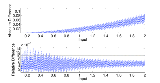
Figure 6: Iteration 4 (last)

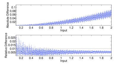
The initial sample S0superscript𝑆0S^{0} is of size 101010. πš–πšŠπš‘π™°πšπšπšŽπš–πš™πšπšœπš–πšŠπš‘π™°πšπšπšŽπš–πš™πšπšœ{\mathtt{maxAttempts}} in the verification routine was also set to 101010. The number of Our algorithm took 4 iterations. We record the intermediate implementations produced by s​y​n​t​h​M​i​n​C​o​s​tπ‘ π‘¦π‘›π‘‘β„Žπ‘€π‘–π‘›πΆπ‘œπ‘ π‘‘synthMinCost in each of the last 3 iterations taken by our algorithm. The initial selected random sample is of size 101010 and the M​A​X​A​T​T​E​M​P​T​S𝑀𝐴𝑋𝐴𝑇𝑇𝐸𝑀𝑃𝑇𝑆MAXATTEMPTS was set to 101010. The number of samples used in each subsequent step of iteration after adding examples discovered by πšπšŽπšœπšπ™΄πš›πš›πšπšŽπšœπšπ™΄πš›πš›\mathtt{testErr} procedure was 18,22182218,22 and 343434. FigureΒ 4,5 and 6 illustrates the error using the intermediate implementations and the final implementation produced by our approach. The wordlengths in FigureΒ 4 are m​y​p​i​(2,3)π‘šπ‘¦π‘π‘–23mypi(2,3), r​a​d​i​u​s​(1,8)π‘Ÿπ‘Žπ‘‘π‘–π‘’π‘ 18radius(1,8), t​(2,11)𝑑211t(2,11), a​r​e​a​(4,11)π‘Žπ‘Ÿπ‘’π‘Ž411area(4,11), those in FigureΒ 5 are m​y​p​i​(2,5)π‘šπ‘¦π‘π‘–25mypi(2,5), r​a​d​i​u​s​(1,8)π‘Ÿπ‘Žπ‘‘π‘–π‘’π‘ 18radius(1,8), t​(2,11)𝑑211t(2,11), a​r​e​a​(4,12)π‘Žπ‘Ÿπ‘’π‘Ž412area(4,12) and in FigureΒ 6 are m​y​p​i​(2,3)π‘šπ‘¦π‘π‘–23mypi(2,3), r​a​d​i​u​s​(1,9)π‘Ÿπ‘Žπ‘‘π‘–π‘’π‘ 19radius(1,9), t​(2,11)𝑑211t(2,11), a​r​e​a​(4,10)π‘Žπ‘Ÿπ‘’π‘Ž410area(4,10). We observe that the number of inputs violating correctness constraint reduces after each iteration. This illustrate how our algorithm works by identifying a few representative inputs violating correctness condition in each iteration and adding that to the set of examples for which we synthesize the least cost implementation.

4.4 Theoretical Results

The following theorem summarizes the correctness and optimality guarantees of our approach.

Theorem 4.1

The synthesis procedure presented in ProcedureΒ 3 is guaranteed to synthesize the fixed-point program which is of minimal cost and satisfies the correctness condition for accuracy if optimization oracles π’ͺSsubscriptπ’ͺ𝑆{\mathcal{O}}_{S} and π’ͺVsubscriptπ’ͺ𝑉{\mathcal{O}}_{V} find globally-optimal solutions (when they exist).

Proof

We first prove correctness and then optimality of the obtained solution. Consider EquationΒ 2:

βˆƒX∈D​o​m​(X)​E​r​r​(Ff​x​(X,πŸπ±β€‹Ο„),Ff​p​(X))>πš–πšŠπš‘π™΄πš›πš›πš˜πš›π‘‹π·π‘œπ‘šπ‘‹πΈπ‘Ÿπ‘Ÿsubscript𝐹𝑓π‘₯π‘‹πŸπ±πœsubscriptπΉπ‘“π‘π‘‹πš–πšŠπš‘π™΄πš›πš›πš˜πš›\exists X\in Dom(X)\;\;Err(F_{fx}(X,{\mathbf{fx\tau}}),F_{fp}(X))>\mathtt{maxError}

If π’ͺVsubscriptπ’ͺ𝑉{\mathcal{O}}_{V} finds globally-optimal solutions, it will find the X∈D​o​m​(X)π‘‹π·π‘œπ‘šπ‘‹X\in Dom(X) that maximizes E​r​r​(Ff​x​(X,πŸπ±β€‹Ο„),Ff​p​(X))πΈπ‘Ÿπ‘Ÿsubscript𝐹𝑓π‘₯π‘‹πŸπ±πœsubscript𝐹𝑓𝑝𝑋Err(F_{fx}(X,{\mathbf{fx\tau}}),F_{fp}(X)), and hence determine where or not EquationΒ 2 is satisfiable. Thus, the correctness condition for accuracy is satisfied.

Next, let πŸπ±β€‹Ο„βˆ—πŸπ±superscript𝜏{\mathbf{fx\tau}}^{*} (β‰ βŠ₯absentbottom\neq\bot) be the fixed-point type returned by ProcedureΒ 3. Let us assume that there exists a fixed-point type πŸπ±β€‹Ο„β€²πŸπ±superscriptπœβ€²{\mathbf{fx\tau}}^{\prime} with a cost lower than πŸπ±β€‹Ο„βˆ—πŸπ±superscript𝜏{\mathbf{fx\tau}}^{*} which also satisfies the correctness condition:

βˆ€X∈D​o​m​(X)​E​r​r​(Ff​x​(X,πŸπ±β€‹Ο„β€²),Ff​p​(X))β‰€πš–πšŠπš‘π™΄πš›πš›πš˜πš›for-allπ‘‹π·π‘œπ‘šπ‘‹πΈπ‘Ÿπ‘Ÿsubscript𝐹𝑓π‘₯π‘‹πŸπ±superscriptπœβ€²subscriptπΉπ‘“π‘π‘‹πš–πšŠπš‘π™΄πš›πš›πš˜πš›\displaystyle\forall X\in Dom(X)\;\;Err(F_{fx}(X,{\mathbf{fx\tau}}^{\prime}),F_{fp}(X))\leq\mathtt{maxError}
∧\displaystyle\land πšŒπš˜πšœπšβ€‹(πŸπ±β€‹Ο„β€²)<πšŒπš˜πšœπšβ€‹(πŸπ±β€‹Ο„βˆ—)𝚌𝚘𝚜𝚝𝐟𝐱superscriptπœβ€²πšŒπš˜πšœπšπŸπ±superscript𝜏\displaystyle{\mathtt{cost}}({\mathbf{fx\tau}}^{\prime})<{\mathtt{cost}}({\mathbf{fx\tau}}^{*})

Hence, for any DβŠ†D​o​m​(X)π·π·π‘œπ‘šπ‘‹D\subseteq Dom(X),

βˆ€X∈D​E​r​r​(Ff​x​(X,πŸπ±β€‹Ο„β€²),Ff​p​(X))β‰€πš–πšŠπš‘π™΄πš›πš›πš˜πš›for-allπ‘‹π·πΈπ‘Ÿπ‘Ÿsubscript𝐹𝑓π‘₯π‘‹πŸπ±superscriptπœβ€²subscriptπΉπ‘“π‘π‘‹πš–πšŠπš‘π™΄πš›πš›πš˜πš›\displaystyle\forall X\in D\;\;Err(F_{fx}(X,{\mathbf{fx\tau}}^{\prime}),F_{fp}(X))\leq\mathtt{maxError}
∧\displaystyle\land πšŒπš˜πšœπšβ€‹(πŸπ±β€‹Ο„β€²)<πšŒπš˜πšœπšβ€‹(πŸπ±β€‹Ο„βˆ—)𝚌𝚘𝚜𝚝𝐟𝐱superscriptπœβ€²πšŒπš˜πšœπšπŸπ±superscript𝜏\displaystyle{\mathtt{cost}}({\mathbf{fx\tau}}^{\prime})<{\mathtt{cost}}({\mathbf{fx\tau}}^{*})

But πŸπ±β€‹Ο„βˆ—πŸπ±superscript𝜏{\mathbf{fx\tau}}^{*} is the solution generated by applying π’ͺSsubscriptπ’ͺ𝑆{\mathcal{O}}_{S} to the optimization problem of EquationΒ 1:

π™Όπš’πš—πš’πš–πš’πš£πšŽβ€‹πšŒπš˜πšœπšβ€‹(πŸπ±β€‹Ο„)β€‹πšœ.𝚝.formulae-sequenceπ™Όπš’πš—πš’πš–πš’πš£πšŽπšŒπš˜πšœπšπŸπ±πœπšœπš\displaystyle\mathtt{Minimize\;\;}{\mathtt{cost}}({\mathbf{fx\tau}})\mathtt{\;\;s.t.}
β‹€x∈SE​r​r​(Ff​x​(x,πŸπ±β€‹Ο„),Ff​l​(x))β‰€πš–πšŠπš‘π™΄πš›πš›πš˜πš›subscriptπ‘₯π‘†πΈπ‘Ÿπ‘Ÿsubscript𝐹𝑓π‘₯π‘₯𝐟𝐱𝜏subscript𝐹𝑓𝑙π‘₯πš–πšŠπš‘π™΄πš›πš›πš˜πš›\displaystyle\displaystyle\bigwedge_{x\in S}Err(F_{fx}(x,{\mathbf{fx\tau}}),F_{fl}(x))\leq\mathtt{maxError} (3)

Since π’ͺSsubscriptπ’ͺ𝑆{\mathcal{O}}_{S} is guaranteed to generate globally-optimal solutions, setting D=S𝐷𝑆D=S, we obtain a contradiction. Hence, there exists no fixed-point type πŸπ±β€‹Ο„β€²πŸπ±superscriptπœβ€²{\mathbf{fx\tau}}^{\prime} with a cost lower than πŸπ±β€‹Ο„βˆ—πŸπ±superscript𝜏{\mathbf{fx\tau}}^{*} which also satisfies the correctness condition. Hence, πŸπ±β€‹Ο„βˆ—πŸπ±superscript𝜏{\mathbf{fx\tau}}^{*} is the optimal correct solution.

As noted earlier, it is difficult to implement ideal π’ͺSsubscriptπ’ͺ𝑆{\mathcal{O}}_{S} and π’ͺVsubscriptπ’ͺ𝑉{\mathcal{O}}_{V} (that find global optima) with current SAT and optimization methods for arbitrary floating-point programs. Nonetheless, our experience with heuristic methods that find local optima has been very good. Also, improvements in optimization/SAT methods can directly be leveraged with our inductive synthesis approach. In contrast, the current techniques for synthesizing fixed-point versions of floating-point programs perform heuristic optimization over a randomly selected set of inputs (see Sec.Β 6 for a detailed discussion). Such techniques do not provide any correctness guarantees and the number of inputs needed could be much larger. Our approach systematically discovers a small number of example inputs such that the optimal fixed-point program for this set yields that for the entire input domain.

5 Experiments

Apart from the running example, we present case studies from DSP and control systems to illustrate the utility of the presented synthesis approach. Our technique was implemented in Matlab, and Nelder-Mead implementation available in Matlab as πšπš–πš’πš—πšœπšŽπšŠπš›πšŒπš‘πšπš–πš’πš—πšœπšŽπšŠπš›πšŒπš‘\mathtt{fminsearch} function was used for numerical optimization. We use the Constantinides et alΒ [6] cost model.

5.1 Running Example

We illustrate the synthesis approach (more details inΒ [13]) presented in SectionΒ 4 using the running example. Our algorithm used 343434 examples and needed 444 iterations. To evaluate our approach, we exhaustively simulated the generated fixed-point program on the given domain (0.1β‰€πš›πšŠπšπš’πšžπšœ<20.1πš›πšŠπšπš’πšžπšœ20.1\leq\mathtt{radius}<2) at intervals of 0.00010.00010.0001. The is presented in FigureΒ 7.

Refer to caption
Figure 7: Our Approach on Running Example.
Refer to caption
Figure 8: Running Example Using Random Inputs.

As a point of comparison, we also show the result of synthesizing a fixed-point program using the πš˜πš™πšπ™Έπš—πšπšžπšŒπšŽπš˜πš™πšπ™Έπš—πšπšžπšŒπšŽ\mathtt{optInduce} routine with 100100100 inputs (333 times as many as our approach) selected uniformly at random (FigureΒ 8). The horizontal line in the plots denotes the maximum error threshold of 0.010.010.01 on the relative difference error function. The cost of the fixed-point program synthesized with random sampling is 89.6589.6589.65, and the fixed-point types of the variables are πŸπ±β€‹Ο„β€‹(πš–πš’πš™πš’)=⟨0,2,3βŸ©πŸπ±πœπš–πš’πš™πš’023{\mathbf{fx\tau}}(\mathtt{mypi})=\langle 0,2,3\rangle, πŸπ±β€‹Ο„β€‹(πš›πšŠπšπš’πšžπšœ)=⟨0,1,8βŸ©πŸπ±πœπš›πšŠπšπš’πšžπšœ018{\mathbf{fx\tau}}(\mathtt{radius})=\langle 0,1,8\rangle, πŸπ±β€‹Ο„β€‹(𝚝)=⟨0,2,10⟩𝐟𝐱𝜏𝚝0210{\mathbf{fx\tau}}(\mathtt{t})=\langle 0,2,10\rangle and πŸπ±β€‹Ο„β€‹(πšŠπš›πšŽπšŠ)=⟨0,4,8βŸ©πŸπ±πœπšŠπš›πšŽπšŠ048{\mathbf{fx\tau}}(\mathtt{area})=\langle 0,4,8\rangle. Notice, however, that it is incorrect for a large number of inputs. In contrast, the cost of the implementation produced using our technique is 104.65104.65104.65, and the fixed-point types of the variables are πŸπ±β€‹Ο„β€‹(πš–πš’πš™πš’)=⟨0,2,3βŸ©πŸπ±πœπš–πš’πš™πš’023{\mathbf{fx\tau}}(\mathtt{mypi})=\langle 0,2,3\rangle, πŸπ±β€‹Ο„β€‹(πš›πšŠπšπš’πšžπšœ)=⟨0,1,9βŸ©πŸπ±πœπš›πšŠπšπš’πšžπšœ019{\mathbf{fx\tau}}(\mathtt{radius})=\langle 0,1,9\rangle, πŸπ±β€‹Ο„β€‹(𝚝)=⟨0,2,11⟩𝐟𝐱𝜏𝚝0211{\mathbf{fx\tau}}(\mathtt{t})=\langle 0,2,11\rangle and πŸπ±β€‹Ο„β€‹(πšŠπš›πšŽπšŠ)=⟨0,4,10βŸ©πŸπ±πœπšŠπš›πšŽπšŠ0410{\mathbf{fx\tau}}(\mathtt{area})=\langle 0,4,10\rangle.

5.2 Infinite Impulse Response (IIR) Filter

The first case study is an IIR filter which is used in digital signal processing applications. It is a first-order direct form-II IIR filter with the schematic shown in FigureΒ 9. The constants are a1=βˆ’0.5subscriptπ‘Ž10.5a_{1}=-0.5, b​0=0.9𝑏00.9b0=0.9 and b​1=0.9𝑏10.9b1=0.9. The fixed-point variables are identified in the schematic. We use our synthesis technique to discover the appropriate fixed-point types of these variables. The input domain used in synthesis is βˆ’2<i​n​p​u​t<22𝑖𝑛𝑝𝑒𝑑2-2<input<2. The correctness condition for accuracy is to ensure that the relative error between the floating-point and fixed-point program is less than 0.10.10.1.

Refer to caption
Figure 9: IIR Filter Schematic
Refer to caption
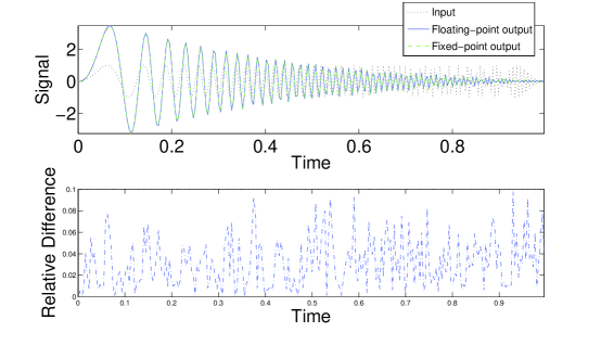
Figure 10: IIR Filter Using Floating-point and Fixed-point. In the top plot, the floating-point and fixed-point outputs are virtually superimposed on each other.

In order to test the correctness of our implementation, we feed a common input signal to both the IIR filter implementations: floating-point version and the fixed-point version obtained by our synthesis technique. The input signal is a linear chirp from 00 to F​s2𝐹𝑠2\frac{Fs}{2} Hz in 111 second.

i​n​p​u​t=(1βˆ’2βˆ’15)Γ—s​i​n​(π×F​s2Γ—t2)𝑖𝑛𝑝𝑒𝑑1superscript215π‘ π‘–π‘›πœ‹πΉπ‘ 2superscript𝑑2input=(1-2^{-15})\times sin(\pi\times\frac{Fs}{2}\times t^{2})

where F​s=256𝐹𝑠256Fs=256 and t=0𝑑0t=0 to 1βˆ’1F​s11𝐹𝑠1-\frac{1}{Fs} and is sampled at intervals of 1F​s1𝐹𝑠\frac{1}{Fs}. FigureΒ 10 shows the input, outputs of both implementations and the relative error between the two outputs. We observe that the implementation satisfies the correctness condition and the relative error remains below 0.10.10.1 throughout the simulation.

5.3 Finite Impulse Response (FIR) Filter

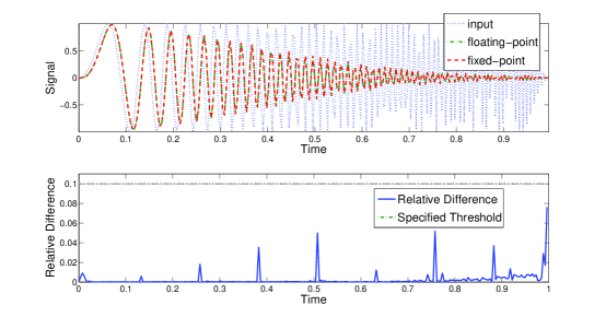
The second case study is a low pass FIR filter of order 4 with tap coefficients 0.0346,0.2405,0.4499,0.24050.03460.24050.44990.24050.0346,0.2405,0.4499,0.2405 and 0.03460.03460.0346. The input domain, correctness condition and input signal to test the floating-point implementation and synthesized fixed-point program are same as the previous case study. FigureΒ 11 shows the input, outputs of both implementations and the relative error between the two outputs. We observe that the implementation satisfies the correctness condition and the relative error remains below 0.10.10.1 throughout the simulation.

Refer to caption
Figure 11: FIR Filter Using Floating-point and Fixed-point. The floating-point/fixed-point outputs are virtually superimposed on each other.

5.4 Field Controlled DC Motor

The next case study is a field controlled DC Motor. It is a classic non-linear control example from KhalilΒ [14]. The example used here is an adaptation of Khalil’s example presented in [claire-course]. The system dynamics is described by the following ordinary differential equations.

vΛ™f=Rf​if+Lf​iΛ™fsubscript˙𝑣𝑓subscript𝑅𝑓subscript𝑖𝑓subscript𝐿𝑓subscript˙𝑖𝑓\displaystyle\dot{v}_{f}=R_{f}i_{f}+L_{f}\dot{i}_{f}
vΛ™a=c1​if​ω+La​iΛ™a+Ra​iasubscriptΛ™π‘£π‘Žsubscript𝑐1subscriptπ‘–π‘“πœ”subscriptπΏπ‘ŽsubscriptΛ™π‘–π‘Žsubscriptπ‘…π‘Žsubscriptπ‘–π‘Ž\displaystyle\dot{v}_{a}=c_{1}i_{f}\omega+L_{a}\dot{i}_{a}+R_{a}i_{a}
J˙​ω˙=c2​if​iaβˆ’c3β€‹Ο‰Λ™π½Λ™πœ”subscript𝑐2subscript𝑖𝑓subscriptπ‘–π‘Žsubscript𝑐3πœ”\displaystyle\dot{J}\dot{\omega}=c_{2}i_{f}i_{a}-c_{3}\omega

The first equation is for the field circuit with vf,if,Rf,Lfsubscript𝑣𝑓subscript𝑖𝑓subscript𝑅𝑓subscript𝐿𝑓v_{f},i_{f},R_{f},L_{f} being its voltage, current, resistance, and inductance. The variables va,ia,Ra,Lasubscriptπ‘£π‘Žsubscriptπ‘–π‘Žsubscriptπ‘…π‘ŽsubscriptπΏπ‘Žv_{a},i_{a},R_{a},L_{a} are the corresponding voltage, current, resistance, and inductance of the armature circuit described by the second equation. The third equation is a torque equation for the shaft, with J𝐽J as the rotor inertia and c3subscript𝑐3c_{3} as a damping coefficient. The term c1​if​ωsubscript𝑐1subscriptπ‘–π‘“πœ”c_{1}i_{f}\omega is the back electromotive force induced in the armature circuit, and c2​if​iasubscript𝑐2subscript𝑖𝑓subscriptπ‘–π‘Žc_{2}i_{f}i_{a} is the torque produced by the interaction of the armature current with the field circuit flux. In the field controlled DC motor, field voltage vfsubscript𝑣𝑓v_{f} is the control input while vasubscriptπ‘£π‘Žv_{a} is held constant. The purpose of the control is to drive the system to the desired set point for the angular velocity Ο‰πœ”\omega.

We can now rewrite the system dynamics in the following normal form where a=RfLfπ‘Žsubscript𝑅𝑓subscript𝐿𝑓a=\frac{R_{f}}{L_{f}}, u=vfLf𝑒subscript𝑣𝑓subscript𝐿𝑓u=\frac{v_{f}}{L_{f}}, b=RaLa𝑏subscriptπ‘…π‘ŽsubscriptπΏπ‘Žb=\frac{R_{a}}{L_{a}}, ρ=vaLa𝜌subscriptπ‘£π‘ŽsubscriptπΏπ‘Ž\rho=\frac{v_{a}}{L_{a}}, c=c1La𝑐subscript𝑐1subscriptπΏπ‘Žc=\frac{c_{1}}{L_{a}}, ΞΈ=c2Jπœƒsubscript𝑐2𝐽\theta=\frac{c_{2}}{J}, d=c3J𝑑subscript𝑐3𝐽d=\frac{c_{3}}{J}.

iΛ™f=βˆ’a​if+usubscriptΛ™π‘–π‘“π‘Žsubscript𝑖𝑓𝑒\displaystyle\dot{i}_{f}=-ai_{f}+u
iΛ™a=βˆ’b​ia+Οβˆ’c​if​ωsubscriptΛ™π‘–π‘Žπ‘subscriptπ‘–π‘ŽπœŒπ‘subscriptπ‘–π‘“πœ”\displaystyle\dot{i}_{a}=-bi_{a}+\rho-ci_{f}\omega
Ο‰Λ™=θ​if​iaβˆ’dβ€‹Ο‰Λ™πœ”πœƒsubscript𝑖𝑓subscriptπ‘–π‘Žπ‘‘πœ”\displaystyle\dot{\omega}=\theta i_{f}i_{a}-d\omega

We assume no damping, that is, c3=0subscript𝑐30c_{3}=0 and set all the other constants a,b,c,ΞΈ,Οπ‘Žπ‘π‘πœƒπœŒa,b,c,\theta,\rho to 111Β [claire-course]. The state feedback law to control the system is given by

u=θ​(a+b)​if​ia+θ​ρ​ifβˆ’c​θ​if2​ωθ​ia+Ο΅π‘’πœƒπ‘Žπ‘subscript𝑖𝑓subscriptπ‘–π‘ŽπœƒπœŒsubscriptπ‘–π‘“π‘πœƒsuperscriptsubscript𝑖𝑓2πœ”πœƒsubscriptπ‘–π‘Žitalic-Ο΅u=\frac{\theta(a+b)i_{f}i_{a}+\theta\rho i_{f}-c\theta i_{f}^{2}\omega}{\theta i_{a}+\epsilon}

where Ο΅=0.01italic-Ο΅0.01\epsilon=0.01 is added to denominator to avoid division by 00. iasubscriptπ‘–π‘Ži_{a} approaches 00 at equilibrium. The corresponding floating-point code is shown below.

0:Β Β πš’πš,πš’πšŠ,Ο‰,ΞΈ,ρ,𝚌,Ο΅subscriptπš’πšsubscriptπš’πšŠπœ”πœƒπœŒπšŒitalic-Ο΅\mathtt{i_{f},i_{a},\omega,\theta,\rho,c,\epsilon}
0:  𝚞𝚞\mathtt{u}
  𝚝𝟷=ΞΈΓ—πš’πšŠπšπŸ·πœƒsubscriptπš’πšŠ\mathtt{t1=\theta\times i_{a}}; 𝚝𝟸=Ο΅+𝚝𝟷𝚝𝟸italic-ϡ𝚝𝟷\mathtt{t2=\epsilon+t1}; 𝚝𝟹=𝟷/𝚝𝟸𝚝𝟹1𝚝𝟸\mathtt{t3=1/t2}; 𝚝𝟹𝟷=𝚊+πš‹πšπŸΉπŸ·πšŠπš‹\mathtt{t31=a+b};
  𝚝𝟹𝟸=πš’πšΓ—πš’πšŠπšπŸΉπŸΈsubscriptπš’πšsubscriptπš’πšŠ\mathtt{t32=i_{f}\times i_{a}}; 𝚝𝟹𝟹=πšπŸΉπŸ·Γ—πšπŸΉπŸΈπšπŸΉπŸΉπšπŸΉπŸ·πšπŸΉπŸΈ\mathtt{t33=t31\times t32}; 𝚝𝟺=ΞΈΓ—πšπŸΉπŸΉπšπŸΊπœƒπšπŸΉπŸΉ\mathtt{t4=\theta\times t33}; 𝚝𝟺𝟷=ΟΓ—πš’πšπšπŸΊπŸ·πœŒsubscriptπš’πš\mathtt{t41=\rho\times i_{f}};
  𝚝𝟻=ΞΈΓ—πšπŸΊπŸ·πšπŸ»πœƒπšπŸΊπŸ·\mathtt{t5=\theta\times t41}; 𝚝𝟼=πš’πšΓ—πš’πšπšπŸΌsubscriptπš’πšsubscriptπš’πš\mathtt{t6=i_{f}\times i_{f}}; 𝚝𝟼𝟷=πšπŸΌΓ—Ο‰πšπŸΌπŸ·πšπŸΌπœ”\mathtt{t61=t6\times\omega}; 𝚝𝟼𝟸=πšπŸΌπŸ·Γ—ΞΈπšπŸΌπŸΈπšπŸΌπŸ·πœƒ\mathtt{t62=t61\times\theta};
  𝚝𝟽=πšŒΓ—πšπŸΌπŸΈπšπŸ½πšŒπšπŸΌπŸΈ\mathtt{t7=c\times t62}; 𝚝𝟾=𝚝𝟺+𝚝𝟻𝚝𝟾𝚝𝟺𝚝𝟻\mathtt{t8=t4+t5}; 𝚝𝟿=πšπŸΎβˆ’πšπŸ½πšπŸΏπšπŸΎπšπŸ½\mathtt{t9=t8-t7}; 𝚞=πšπŸΉΓ—πšπŸΏπšžπšπŸΉπšπŸΏ\mathtt{u=t3\times t9};
  return  𝚞𝚞\mathtt{u}

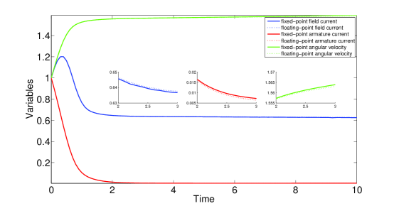
The system is initialized with field current if=1subscript𝑖𝑓1i_{f}=1, armature current ia=1subscriptπ‘–π‘Ž1i_{a}=1 and angular velocity Ο‰=1πœ”1\omega=1.

Refer to caption
Figure 12: DC Motor Using Floating-point and Fixed-point Controller with zoomed-in view for 222 to 333 seconds.

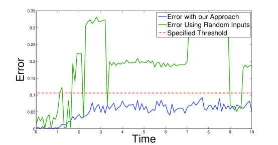
The computed control law can be mathematically shown to be correct by designers who are more comfortable in reasoning with real arithmetic but not with finite precision arithmetic. Its implementation using floating-point computation also closely mimics the arithmetic in reals but the control algorithms are often implemented using fixed-point computation on embedded platforms. We use our synthesis technique to automatically derive a low cost fixed-point implementation of the control law computing u𝑒u. The input domain is 0≀ia,if,ω≀1.5formulae-sequence0subscriptπ‘–π‘Žsubscriptπ‘–π‘“πœ”1.50\leq i_{a},i_{f},\omega\leq 1.5. The correctness condition for accuracy is that the absolute difference between the u𝑒u computed by fixed-point program and the floating-point program is less than 0.10.10.1.

FigureΒ 12 shows the simulation of the system using the fixed-point implementation of the controller and the floating-point implementation. This end-to-end simulation shows that fixed-point program generated by our technique can be used to control the system as effectively as the floating-point program. This illustrates the practical utility of our technique. FigureΒ 13 plots the difference between the control input computed by the fixed-point program and the floating-point program. It shows that the fixed-point types synthesized using our approach satisfy the correctness condition, and the difference between the control input computed by the fixed-point and floating-point program is within the specified maximum error threshold of 0.10.10.1. The number of inputs needed in our approach was 127127127. In contrast, the fixed-point types found using 635635635(5X our approach) randomly selected inputs violate the correctness condition for a large number of inputs.
Refer to caption
Figure 13: Error in Control Input Using Fixed-point and Floating-point Program

5.5 Two-Wheeled Welding Mobile Robot

The next case study is a nonlinear controller for a two-wheeled welding mobile robot (WMR)Β [3]. The robot consists of two wheels and a robotic arm. The wheels can roll and there is no slipping. (x,y)π‘₯𝑦(x,y) represents the Cartesian coordinate of the WMR’s center point and Ο•italic-Ο•\phi is the heading angle of the WMR. v𝑣v and Ο‰πœ”\omega are the straight and angular velocities of the WMR at its center point. The welding point coordinates (xw,yw)subscriptπ‘₯𝑀subscript𝑦𝑀(x_{w},y_{w}) and the heading angle Ο•wsubscriptitalic-ϕ𝑀\phi_{w} can be calculated from the WMR’s center point:

xw=xβˆ’l​sin⁑ϕsubscriptπ‘₯𝑀π‘₯𝑙italic-Ο•\displaystyle x_{w}=x-l\sin\phi
yw=y+l​cos⁑ϕsubscript𝑦𝑀𝑦𝑙italic-Ο•\displaystyle y_{w}=y+l\cos\phi
Ο•w=Ο•subscriptitalic-ϕ𝑀italic-Ο•\displaystyle\phi_{w}=\phi

So, the equation of motion for the welding point is as follows:

xΛ™w=v​cosβ‘Ο•βˆ’l​ω​cosβ‘Ο•βˆ’l˙​sin⁑ϕsubscriptΛ™π‘₯𝑀𝑣italic-Ο•π‘™πœ”italic-ϕ˙𝑙italic-Ο•\displaystyle\dot{x}_{w}=v\cos\phi-l\omega\cos\phi-\dot{l}\sin\phi
yΛ™w=v​sinβ‘Ο•βˆ’l​ω​sin⁑ϕ+l˙​cos⁑ϕsubscript˙𝑦𝑀𝑣italic-Ο•π‘™πœ”italic-ϕ˙𝑙italic-Ο•\displaystyle\dot{y}_{w}=v\sin\phi-l\omega\sin\phi+\dot{l}\cos\phi
Ο•Λ™w=Ο‰subscriptΛ™italic-Ο•π‘€πœ”\displaystyle\dot{\phi}_{w}=\omega

The objective of the WMR controller is to ensure that the robot tracks a reference point R. The reference point R moving with a constant velocity of vrsubscriptπ‘£π‘Ÿv_{r} on the reference path has coordinates (xr,yr)subscriptπ‘₯π‘Ÿsubscriptπ‘¦π‘Ÿ(x_{r},y_{r}) and the heading angle Ο•rsubscriptitalic-Ο•π‘Ÿ\phi_{r}. The tracking error is the difference between the location of the robot and the reference point.

[e1e2e3]=[cos⁑ϕsin⁑ϕ0βˆ’sin⁑ϕcos⁑ϕ0001]​[xrβˆ’xwyrβˆ’ywΟ•rβˆ’Ο•w]delimited-[]subscript𝑒1subscript𝑒2subscript𝑒3delimited-[]italic-Ο•italic-Ο•0italic-Ο•italic-Ο•0001delimited-[]subscriptπ‘₯π‘Ÿsubscriptπ‘₯𝑀subscriptπ‘¦π‘Ÿsubscript𝑦𝑀subscriptitalic-Ο•π‘Ÿsubscriptitalic-ϕ𝑀\left[{\begin{array}[]{c}e_{1}\\ e_{2}\\ e_{3}\end{array}}\right]=\left[{\begin{array}[]{ccc}\cos\phi&\sin\phi&0\\ -\sin\phi&\cos\phi&0\\ 0&0&1\\ \end{array}}\right]\left[{\begin{array}[]{c}x_{r}-x_{w}\\ y_{r}-y_{w}\\ \phi_{r}-\phi_{w}\end{array}}\right]

The two control parameters in the model are v𝑣v and Ο‰πœ”\omega. In order to ensure that the error quickly converges to 00, a nonlinear controller based on Lyapunov stability is as follows:

v=l​(Ο‰r+k2​e2​vr+k3​sin⁑e3)+vr​cos⁑e3+k1​e1𝑣𝑙subscriptπœ”π‘Ÿsubscriptπ‘˜2subscript𝑒2subscriptπ‘£π‘Ÿsubscriptπ‘˜3subscript𝑒3subscriptπ‘£π‘Ÿsubscript𝑒3subscriptπ‘˜1subscript𝑒1\displaystyle v=l(\omega_{r}+k_{2}e_{2}v_{r}+k_{3}\sin e_{3})+v_{r}\cos e_{3}+k_{1}e_{1}
Ο‰=Ο‰r+k2​e2​vr+k3​sin⁑e3πœ”subscriptπœ”π‘Ÿsubscriptπ‘˜2subscript𝑒2subscriptπ‘£π‘Ÿsubscriptπ‘˜3subscript𝑒3\displaystyle\omega=\omega_{r}+k_{2}e_{2}v_{r}+k_{3}\sin e_{3}

where k1,k2subscriptπ‘˜1subscriptπ‘˜2k_{1},k_{2} and k3subscriptπ‘˜3k_{3} are positive constants. TableΒ 3 provides the numerical values of constants and initial values of the state variables from Bui et alΒ [3]. All lengths are in meters, angle in radians and time in seconds.

Table 3: Numerical and Constant Values
Parameters Values Parameters Values
k1subscriptπ‘˜1k_{1} 4.24.24.2 l𝑙l 0.150.150.15
k2subscriptπ‘˜2k_{2} 500050005000 l˙˙𝑙\dot{l} 00
k3subscriptπ‘˜3k_{3} 111 vrsubscriptπ‘£π‘Ÿv_{r} 7.5​eβˆ’37.5𝑒37.5e-3
xrsubscriptπ‘₯π‘Ÿx_{r} 0.2800.2800.280 xwsubscriptπ‘₯𝑀x_{w} 0.2700.2700.270
yrsubscriptπ‘¦π‘Ÿy_{r} 0.4000.4000.400 ywsubscript𝑦𝑀y_{w} 0.3900.3900.390
Ο•italic-Ο•\phi 00 Ο•wsubscriptitalic-ϕ𝑀\phi_{w} 151515
Refer to caption
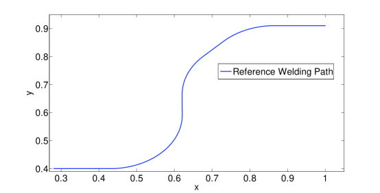
Figure 14: Reference Welding Line
Refer to caption
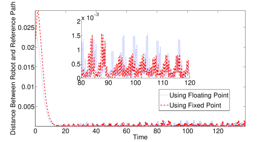
Figure 15: Distance of WMR from Reference Line with zoomed-in view for 808080 to 120120120 seconds.
Refer to caption
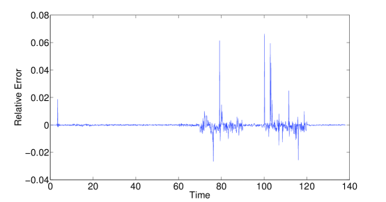
Figure 16: Error in computing v𝑣v
Refer to caption
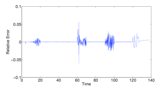
Figure 17: Error in computing Ο‰πœ”\omega

We use our synthesis technique to automatically synthesize fixed-point program computing both control inputs: v𝑣v and Ο‰πœ”\omega. The error function used for v𝑣v is the relative difference

vf​l​o​a​t​i​n​gβˆ’p​o​i​n​tβˆ’vf​i​x​e​dβˆ’p​o​i​n​tvf​l​o​a​t​i​n​gβˆ’p​o​i​n​tsubscriptπ‘£π‘“π‘™π‘œπ‘Žπ‘‘π‘–π‘›π‘”π‘π‘œπ‘–π‘›π‘‘subscript𝑣𝑓𝑖π‘₯π‘’π‘‘π‘π‘œπ‘–π‘›π‘‘subscriptπ‘£π‘“π‘™π‘œπ‘Žπ‘‘π‘–π‘›π‘”π‘π‘œπ‘–π‘›π‘‘\frac{v_{floating-point}-v_{fixed-point}}{v_{floating-point}}

and the error function used for Ο‰πœ”\omega is the moderated relative difference

Ο‰f​l​o​a​t​i​n​gβˆ’p​o​i​n​tβˆ’Ο‰f​i​x​e​dβˆ’p​o​i​n​tΟ‰f​l​o​a​t​i​n​gβˆ’p​o​i​n​t+Ξ΄subscriptπœ”π‘“π‘™π‘œπ‘Žπ‘‘π‘–π‘›π‘”π‘π‘œπ‘–π‘›π‘‘subscriptπœ”π‘“π‘–π‘₯π‘’π‘‘π‘π‘œπ‘–π‘›π‘‘subscriptπœ”π‘“π‘™π‘œπ‘Žπ‘‘π‘–π‘›π‘”π‘π‘œπ‘–π‘›π‘‘π›Ώ\frac{\omega_{floating-point}-\omega_{fixed-point}}{\omega_{floating-point}+\delta}

where Ξ΄=0.001𝛿0.001\delta=0.001. The moderated relative difference is useful here since Ο‰f​l​o​a​t​i​n​gβˆ’p​o​i​n​tsubscriptπœ”π‘“π‘™π‘œπ‘Žπ‘‘π‘–π‘›π‘”π‘π‘œπ‘–π‘›π‘‘\omega_{floating-point} can be 00. We require that the difference values for both controllers are less than 0.10.10.1. FigureΒ 14 shows the reference line for welding and FigureΒ 15 shows the distance of the WMR from the reference line as a function of time for both cases: firstly, when the controller is implemented as a floating-point program and secondly, when the controller is implemented as a fixed-point program synthesized using our technique. The robot starts a little away from the reference line but quickly starts tracking the line in both cases. FigureΒ 16 and FigureΒ 17 show the error between the floating-point controller and fixed-point controller for both control inputs: v𝑣v and Ο‰πœ”\omega, respectively.

TableΒ 4 summarizes the performance of our technique in the four case-studies.

Table 4: Performance
Case-study Runtime (seconds) # of Iterations
IIR Filter 268 5
FIR Filter 379 4
DC Motor u𝑒u 4436 8
WMR v𝑣v 2218 7
Ο‰πœ”\omega 1720 4

6 Related Work

Previous techniques for optimizing fixed-point types are based on statistical sampling of the input space. These methods sample a large number of inputs and heuristically solve an optimization problem that minimizes implementation cost while ensuring that some correctness specification is met over the sampled inputs. The techniques differ in in the heuristic search method employed, in the measure of cost, or in how accuracy of fixed-point implementation is determined. Sung and KumΒ [22] use a heuristic search technique which starts with the minimum wordlength implementation as the initial guess. The wordlengths are increased one by one till the error falls below an acceptable threshold. Han et al.Β [10, 11] use a gradient-based sequential search method which starts with the minimum wordlength implementation as the initial guess. The gradient (ratio of increase in accuracy and increase in wordlengths) is computed for a set of wordlength changes at each step and the search moves in the direction with maximum gradient. Shi et al.Β [20] propose a floating-point to fixed-point conversion methodology for digital VLSI signal processing systems. Their approach is based on a perturbation theory which shows that the change to the first order is a linear combination of all the first- and second-order statistics of the quantization noise sources. Their technique works with general specification critera, as long as these can be represented as large ensemble averages of functions of the signal outputs. For example, they use mean-squared error (MSE) as the specification function. The cost of the implementation is a quadratic function. Monte Carlo simulation of a large number of input examples is used to formulate a quadratic optimization problem based on perturbation theory. In contrast, our specification requires that the accuracy condition holds for all inputs and not just on an average. Further, the cost function can be any arbitrary function for our technique and need not be quadratic. Perhaps most importantly, our technique does not rely on apriori random sampling of a large number of input values, instead using optimization to discover a small set of interesting examples which suffice to discover optimal fixed-point implementation.

Purely analytical methodsΒ [21, 15] based on dataflow analysis have also been proposed for synthesizing fixed-point programs based on forward and backward propagation in the program’s dataflow graph. The advantages of these techniques are that they do not rely on picking the right inputs for simulation, can handle arbitrary programs (with approximation), and can provide correctness guarantees. However, they tend to produce very conservative wordlength results.

Inductive synthesis based on satisfiability solving has been previously used for synthesizing programs from functional specifications. These approachesΒ [12, 9] rely on constraint solving in much the same way as we rely on optimization routines. However, these approaches only seek to find a correct program, without any notion of cost and optimization. In contrast, our technique is used to find a fixed-point program which is not only correct with respect to a condition on accuracy but is also of minimal cost.

7 Conclusion

In this paper, we presented a novel approach to automated synthesis of fixed-point program from floating-point program by discovering the fixed-point types of the variables. The program is synthesized to satisfy the provided correctness condition for accuracy and to have optimal cost with respect to the provided cost model.

References

  • [1] ANSI/IEEE Std. 754-1985: IEEE standard for binary floating-point arithmetic.
  • [2] Matlab: Fixed-point toolbox.
  • [3] T.H. Bui, T.T. Nguyen, T.L. Chung, and S.B. Kim. A simple nonlinear control of a two-wheeled welding mobile robot. Int. Journal of Control, Automation and Systems, 1, 2003.
  • [4] Swarat Chaudhuri, Sumit Gulwani, and Roberto Lublinerman. Continuity analysis of programs. In POPL ’10, pages 57–70, 2010.
  • [5] JonathanΒ A. Clarke, AltafΒ Abdul Gaffar, GeorgeΒ A. Constantinides, and Peter Y.Β K. Cheung. Fast word-level power models for synthesis of FPGA-based arithmetic. In ISCAS, 2006.
  • [6] GeorgeΒ A. Constantinides, Peter Y.Β K. Cheung, and Wayne Luk. Wordlength optimization for linear digital signal processing. In IEEE Transactions on Computer-Aided Design of Integrated Circuits and Systems, Vol 22, No. 10, pages 1432–1443, 2003.
  • [7] R.Β Fletcher. Practical Methods of Optimization. J. Wiley, 1986.
  • [8] David Goldberg. What every computer scientist should know about floating-point arithmetic. ACM Computing Surveys, 23:5–48, 1991.
  • [9] Sumit Gulwani, Susmit Jha, Ashish Tiwari, and Ramarathnam Venkatesan. Synthesis of loop-free programs. In PLDI, pages 62–73, 2011.
  • [10] Kyungtae Han, Iksu Eo, Kyungsu Kim, and Hanjin Cho. Numerical word-length optimization for cdma demodulator. In ISCAS 2001, volumeΒ 4, pages 290 –293 vol. 4, may 2001.
  • [11] Kyungtae Han and B.L. Evans. Wordlength optimization with complexity-and-distortion measure and its application to broadband wireless demodulator design. In IEEE International Conference on Acoustics, Speech, and Signal Processing, 2004, volumeΒ 5, pages V – 37–40 vol.5, may 2004.
  • [12] Susmit Jha, Sumit Gulwani, Sanjit Seshia, and Ashish Tiwari. Oracle-guided component-based program synthesis. In ICSE, pages 215–224, 2010.
  • [13] Susmit Jha and SanjitΒ A. Seshia. SWATI: Synthesizing wordlengths automatically using testing and induction. UC Berkeley Technical Report, pages TR–XX, 2013.
  • [14] H.K. Khalil. Nonlinear systems. Macmillan Pub. Co., 1992.
  • [15] Seehyun Kim, Ki-Il Kum, and Wonyong Sung. Fixed-point optimization utility for c and c++ based digital signal processing programs. Circuits and Systems II: Analog and Digital Signal Processing, IEEE Transactions on, 45(11):1455 –1464, nov 1998.
  • [16] Mike Tien-Chien Lee, V.Β Tiwari, S.Β Malik, and M.Β Fujita. Power analysis and minimization techniques for embedded DSP software. Very Large Scale Integration (VLSI) Systems, IEEE Transactions on, 5(1):123 –135, march 1997.
  • [17] E.Β Macii, M.Β Pedram, and F.Β Somenzi. High-level power modeling, estimation, and optimization. Computer-Aided Design of Integrated Circuits and Systems, IEEE Transactions on, 17(11):1061 –1079, nov 1998.
  • [18] Rupak Majumdar and Indranil Saha. Symbolic robustness analysis. In RTSS ’09, pages 355–363, 2009.
  • [19] J.Β A. Nelder and R.Β Mead. A simplex method for function minimization. The Computer Journal, 7(4):308–313, January 1965.
  • [20] Changchun Shi and RobertΒ W. Brodersen. An automated floating-point to fixed-point conversion methodology. In Proc. IEEE Int. Conf. on Acoust., Speech, and Signal Processing, pages 529–532, 2003.
  • [21] Mark Stephenson, Jonathan Babb, and Saman Amarasinghe. Bidwidth analysis with application to silicon compilation. SIGPLAN Not., 35:108–120, May 2000.
  • [22] Wonyong Sung and Ki-Il Kum. Simulation-based word-length optimization method for fixed-point digital signal processing systems. Signal Processing, IEEE Transactions on, 43(12):3087 –3090, dec 1995.
  • [23] Randy Yates. Fixed-point arithmetic: An introduction. In Technical Reference Digital Signal Labs, 2009.