Variability of Hypervelocity Stars

Abstract

We present time-series photometry of 11 hypervelocity stars (HVSs) to constrain their nature. Known HVSs are mostly late-B spectral type objects that may be either main-sequence (MS) or evolved blue horizontal branch (BHB) stars. Fortunately, MS stars at these effective temperatures, $T_{eff}\sim$ 12,000 K, are good candidates for being a class of variable stars known as slowly pulsating B stars (SPBs). We obtained photometry on four nights at the WIYN 3.5 m telescope, and on six nights on the 2.4 m Hiltner telescope. Using sinusoidal fits, we constrain four of our targets to have periods between $P\sim 0.2-2$ days, with a mean value of 0.6 days. Our amplitudes vary between $A=0.5-3$%. This suggests that these four HVSs are SPBs. We discuss a possible origin for these stars, and why further observations are necessary.

1. Introduction

Hills (1988) theorized that a binary star system disrupted by a massive black hole (MBH) could result in the unbound ejection of one component as a HVS. Brown et al. (2005) discovered the first HVS in the Galactic halo, and currently over 20 HVSs have been identified in the Milky Way (Edelmann et al. 2005; Hirsch et al. 2005; Brown et al. 2006a; Brown et al. 2006b; Brown et al. 2007; Brown et al. 2009; Brown et al. 2012b). Due to their large distances, the nature of the HVSs can be difficult to determine. One useful technique is time-series photometry, however before this paper only HVS1 had been thus observed (Fuentes et al., 2006, hereafter F06). This paper present the results of time-series photometry for 11 HVSs.

The Milky Way houses Sgr A*, a massive black hole (MBH) of $\sim 4\times 10^{6}$ M_⊙ (e.g. Ghez et al. 2005; Ghez et al. 2008; Gillessen et al. 2009a). In Hill’s scenario, HVSs are a natural consequence of a binary star system interacting with this MBH. However, a number of different mechanisms have been proposed to produce HVSs, including the inspiral of an intermediate-mass black hole (Yu & Tremaine 2003; Sesana et al. 2009), the disruption of a triple-star system (Perets 2009b; Ginsburg & Perets 2011), and interactions between stars and stellar-mass black holes (O’Leary & Loeb, 2008). Observational and theoretical evidence point to the Hill’s mechanism as the most likely source for these HVSs (e.g. Ginsburg & Loeb 2006; Perets 2009a; Brown et al. 2010; Brown et al. 2012a). Simulations show that when a HVS is produced, the companion is left in a highly eccentric orbit around Sgr A*. This agrees with the known orbits of a number of stars observed orbiting within 1″  of Sgr A* (e.g. Schödel et al. 2003; Ghez et al. 2005), thereby suggesting that some of the stars nearest Sgr A* (so-called S-stars), are former companions to HVSs (Ginsburg & Loeb, 2006). Simulations further show that a binary star system disrupted by the MBH may result in a collision between the two stars, and if the collisional velocity is small enough the system may coalesce (Ginsburg & Loeb 2007; Antonini et al. 2011). HVSs may also be used to probe the shape of the Galactic halo (Gnedin et al., 2005), and they may even house planets (Ginsburg et al., 2012).

Consequently, HVSs offer a wealth of knowledge, and it is important to understand their nature. One difficulty is that HVSs may be MS or evolved BHB stars. Known HVSs are late-B spectral type objects, and MS and BHB stars at this T${}_{eff}\sim 12,000$ K have very similar surface gravities. Depending on their nature, the intrinsic luminosity of an observed HVS may differ by a factor of $\sim 4$ and consequently the estimated distances to the HVS may differ by a factor of $\sim 2$. The ages may also differ by as much as an order of magnitude. Using the present-day stellar mass function, Demarque & Virani (2007) argue that HVSs are most likely evolved low-mass stars. However, echelle spectroscopic observations indicate that HVS3 is a MS B star of M $\sim 9$ M_⊙ (Edelmann et al. 2005; Przybilla et al. 2008a; Bonanos et al. 2008) while HVS5, HVS7 and HVS8 are MS stars of M $\sim 3.5$ M_⊙ each (Brown et al. 2012a; Przybilla et al. 2008b; López-Morales & Bonanos 2008).

The remaining HVSs are too faint to be studied with echelle spectroscopy with existing telescopes. However, the effective temperature of HVSs makes them candidates for being SPBs. SPBs were first introduced by Waelkens (1991) who found seven intermediate B-type stars with photometric variations of a few millimagnitudes (mmag) and periods of $\sim 1$ day. This variability is due to $g$-mode pulsations, which are believed to be driven by the $\kappa$-mechanism (e.g. Dziembowski et al. 1993; Gautschy & Saio 1995). Observed SPBs have periods 0.5-4 days, spectral range between B2 and B9, masses 3-7 M_⊙ , and T_eff = 12,000-18,000 K (Waelkens 1991; Waelkens et al. 1998; Gautschy & Saio 1996; De Cat & Aerts 2002). Furthermore, all SPBs are observed to be slow rotators although why this is the case is not well understood (Ushomirsky & Bildsten, 1998).

BHB stars are bluewards of the RR Lyrae instability strip and are not observed to pulsate (Contreras et al. 2005; Catelan 2009). Consequently, the detection of mmag variability with a period of $\sim 1$ day is indicative of a SPB, and are the two observable properties we are seeking. F06 found a period for HVS1 consistent with that of a SPB. However, Turner et al. (2009) argue that the observed decrease in brightness of HVS1 may be due to extinction.

To check for variability we took time-series photometry of 11 HVSs over the course of four nights on the WIYN 3.5 m telescope and follow-up observations over the course of six more nights on the Hiltner 2.4 m telescope. In §2 we discuss our observations. In §3 we discuss our analysis. We conclude our results in §4.

2. Observations

2.1. WIYN Observations

The first set of observations were taken the nights of 2012 February 23 – 26 with the Mini-Mosaic Imager (Saha et al., 2000) at the 3.5 m WIYN telescope at Kitt Peak National Observatory. All observations were in the SDSS g-band, and the results are summarized in Table 1. The Mini-Mosaic Imager has a field of view of 9.6′  $\times$ 9.6′  with 0.141 arcsec pixel^-1. Our goal was to detect photometric variability to within a few percent amplitude. In order to obtain enough photon statistics, faint objects such as HVS1 required longer exposure times, up to 1200 s, while brighter objects such as HVS5 had exposure times as short as 300 s. This provided high signal-to-noise ratio (S/N) $\sim 100-200$. We measured the photometry differentially using nearby stars of similar colors to within $\sim 0.6$ mag in $(g-r)$, identified by Sloan Digital Sky Survey photometry (SDSS; York et al. 2000). The raw images were reduced in IRAF (see Tody 1993) using ccdproc. Photometry was analyzed using package DAOPHOT (Stetson, 1987) and SExtractor (Bertin & Arnouts, 1996).

2.2. MDM Observations

The second set of observations were taken the nights of 2012 May 11 – 16 with the 4K imager at the 2.4 m Hiltner telescope at the MDM Observatory. All observations were in the Johnson B-band, and the results are summarized in Table 1. Conversion between $B$ and $g$ is given in a number of papers (e.g. Jester et al. 2005; Karaali et al. 2005). Since we chose the standards and targets to have similar colors to within $\sim 0.6$ mag in $(g-r)$, any systematic differences will be minimal and have no affect on our overall results. The 4K imager has a field of view of 21.3′  $\times$ 21.3′  with 0.315 arcsec pixel^-1. We concentrated on the five HVSs that based upon our first observations appeared to be variable (in Table 1). The MDM data have significantly lower precision since most of our targets set early in May and the higher airmasses led to poorer seeing. We reduced our 4K data using software pipeline developed by Jason Eastman. We then analyzed our photometry in the same manner as that of our first set of observations.

Our errors are limited by photon statistics. Typical errors for our measurement with the WIYN are $\sim 0.5$%. The Hiltner data are substantially poorer with errors $\sim 3$% or larger. These large errors do not offer additional constraints on the HVSs, and thus are omitted from the calculations. Nevertheless the Hiltner measurements do provide a consistency check for our WIYN data, and we discuss them in more detail with regards to HVS5 and HVS7. We take 0.01 mag as the threshold for a significant detection of variability.

Table 1Summary of Observations

Star	WIYN Images	Variable?	MDM Images
HVS1	12	Yes	6
HVS4	10	Yes	6
HVS5	12	Yes	13
HVS6	8	No	-
HVS7	8	Yes	12
HVS8	8	No	-
HVS9	8	No	-
HVS10	8	No	-
HVS11	7	No	-
HVS12	7	No	-
HVS13	7	Yes	6

Note. — The leftmost column is the target, followed by the number of exposures taken with the WIYN 3.5 m telescope (column 2), whether the data show any variability (column 3), and the number of exposures taken in follow-up observations done with the Hiltner 2.4 m telescope (column 4).

3. Results

Of the 11 HVSs observed using the WIYN 3.5 m telescope, we find three HVSs with significant variability, one HVS with possible variability, and HVS5 is ambiguous. In all cases the period of variability is consistent with that of SPBs (see Table 2). For each star, we fit our data to the model

$$y=A\,sin[2\pi ft_{i}+\phi].$$ (1)

where $A$ is the amplitude, $f$ the frequency, and $\phi$ our phase at time $t_{i}$. We consider periods in the range $3<P<120$ hours. Periods shorter than three hours are not meaningful, since our observations for each HVS were taken no less than a few hours apart. Similarly, the period must be less than five days since our observing program on the WIYN was a total of 4 nights. We constrain the amplitude to be $0.005\leq A\leq 0.05$ which is consistent with our errors. We plot $\chi^{2}$ versus frequency for the five HVSs that showed possible variability.

As noted by Turner et al. (2009), atmospheric extinction diminishes the brightness of blue stars more than that of red stars. For our differential photometry we choose stars with similar color to within $\sim 0.6$ mag in $(g-r)$ of our target HVSs. We examined the dependence of our observations on airmass and observed a nearly zero mag deviation in relative photometry for all targets except HVS1 which showed a very slight slope. Consequently, a comparison star of redder color would produce a significant difference in relative photometry (see Figure 1).

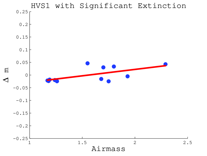
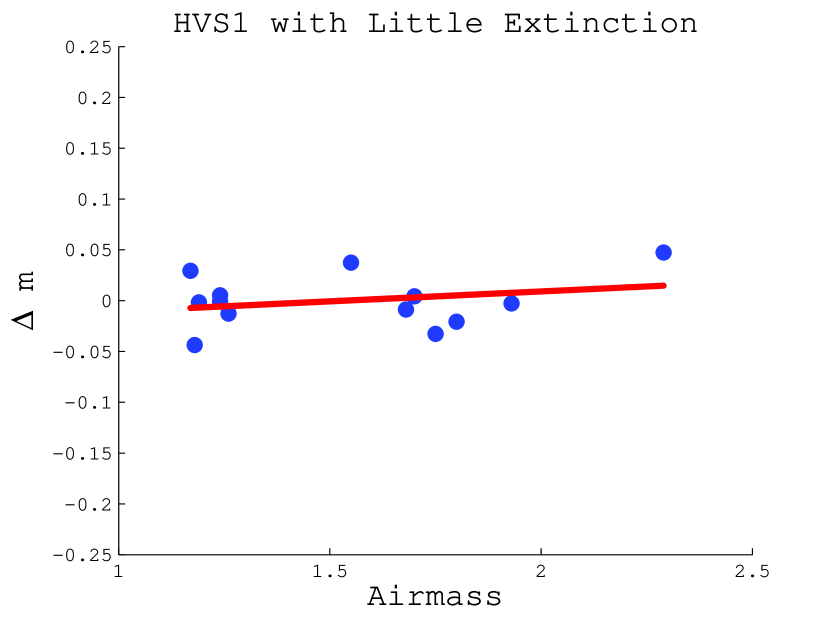
Figure 1.— The effect of airmass on observations is demonstrated here. Straight lines are best fits to the data. Note that HVS1 has $g-r$ = -0.2391. Top: relative photometry of HVS1 versus airmass for a star with $g-r$ = 0.6907. Extinction produces a systematic difference in relative photometry of $\sim$ 0.05 mag. Bottom: relative photometry of HVS1 versus airmass for a star with $g-r$ = 0.2673. Extinction produces a systematic difference in relative photometry of $<$ 0.01 mag. Note that for our other targets, the systematic difference was significantly less than 0.01 mag. The color values were retrieved from SDSS (http://skyserver.sdss3.org/DR8/en/tools/search/IQS.asp)

In order to determine the significance of our detections, we looked at a few goodness of fit tests. The $\chi^{2}$ distribution is useful, but can be ambiguous. However, the well known $F$-test looks at two populations according to the $F$ distribution given by

$$F=\frac{\chi^{2}_{1}/\nu_{1}}{\chi^{2}_{2}/\nu_{2}}$$ (2)

where $f$ is our function and $\nu_{1}$ and $\nu_{2}$ are the degrees of freedom corresponding to $\chi^{2}_{1}$ and $\chi^{2}_{2}$ (Bevington & Robinson, 2003). We calculate $\chi^{2}_{1}$ for $y=0$ and compare it with $\chi^{2}_{2}$ obtained by fitting our best fit values into equation 1. Our results are summarized in Table 2. In the following, we give notes on the individual stars. Error bars for the period and amplitude were obtained using Monte Carlo methods and then calculating the RMS.

3.1. HVS1

Before our measurements, HVS1 was the only HVS with time-series photometry. F06 carried out their observations over two nights with the 6.5 m telescope on the MMT followed by four nights with the 1.2 m telescope at FLWO. They obtained both $g$ and $r$-band images. Although they found no variability in the $r$-band, they did find significant variability in the $g$-band. When comparing results, we find that our best fit amplitude of $A=0.02878\pm 0.00156$ mag agrees well with F06 who found $A=0.0280\pm 0.0033$ mag. If we calculate our differential photometry using a star with $g-r$ significantly larger than HVS1 (see the top panel of Figure 1) we find a best fit period of $P=0.34567$ days which agrees to within 3% with F06 who found $P=0.355$ days. However, if atmospheric extinction is taken into account and we use a star with $g-r$ closer to that of HVS1 (see the bottom panel of Figure 1), our most significant period is $P=0.72738\pm 0.00767$ days. Note that $P\sim 0.35$ days is our second most significant period given our data. Figure 2 shows our relative photometry for HVS1 and our periodogram. Our $\chi^{2}_{min}$ = 45.5 for 10 degrees of freedom. Figure 3 shows our best fit model with our WIYN data folded about our best fit period. Our $F$-test resulted in a value of 0.0825 which has significance at the 1.6-sigma level.

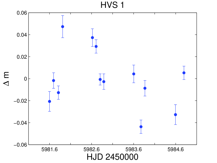
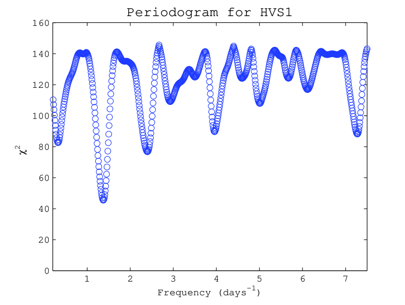
Figure 2.— Results for HVS1. Top: relative photometry of HVS1 with data taken from the WIYN 3.5 m telescope. For convenience the photometry was rescaled to have a mean of zero. This is $g$-band vs. HJD-2,450,000. Bottom: $\chi^{2}$ as a function of period (days). The best-fit model gives $P=0.72738\pm 0.00767$ days.

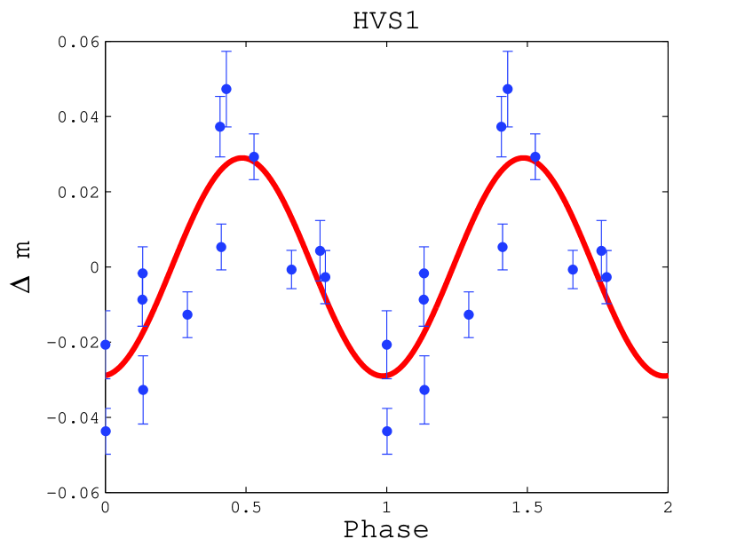
Figure 3.— Relative photometry of HVS1 as a function of phase angle. The light curve is folded according to the best-fit model with $P=0.72738$ days.

3.2. HVS4

We find a best fit period of $P=0.18212\pm 0.00057$ days. However, there are strong aliases ranging from $P\sim 0.15-2$ days. Our best fit amplitude is $A$ = 0.00672 $\pm 0.00064$ mag. Our $\chi^{2}_{min}$ = 12.5 for 7 degrees of freedom. Figure 4 shows our relative photometry for HVS4 and our periodogram. Figure 5 shows our best fit model with our WIYN data folded about our best fit period. Our $F$-test resulted in probability of 0.0463 which is significant at the two-sigma level.

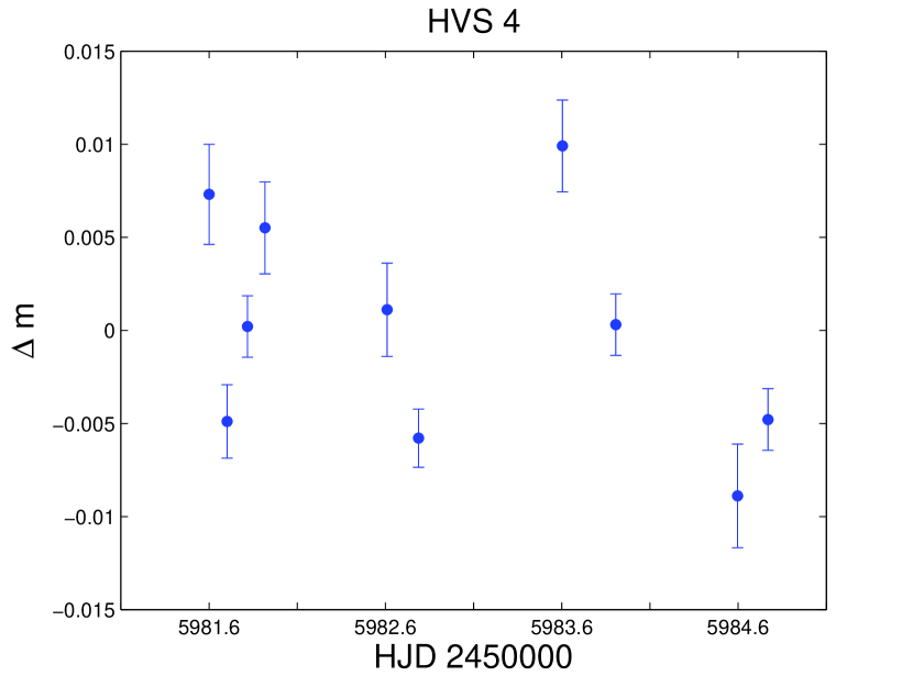
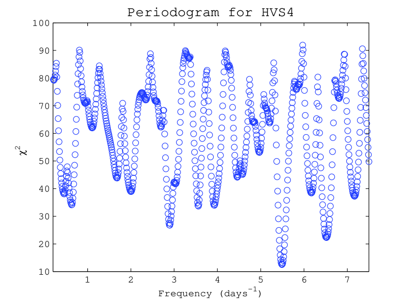
Figure 4.— Results for HVS4. Top: relative photometry of HVS4 with data taken from the WIYN 3.5 m telescope. For convenience the photometry was rescaled to have a mean of zero. This is $g$-band vs. HJD-2,450,000. Bottom: $\chi^{2}$ as a function of period (days). The best-fit model gives $P=0.18212\pm 0.00057$ but we have aliases up to $P\sim 2$ days.

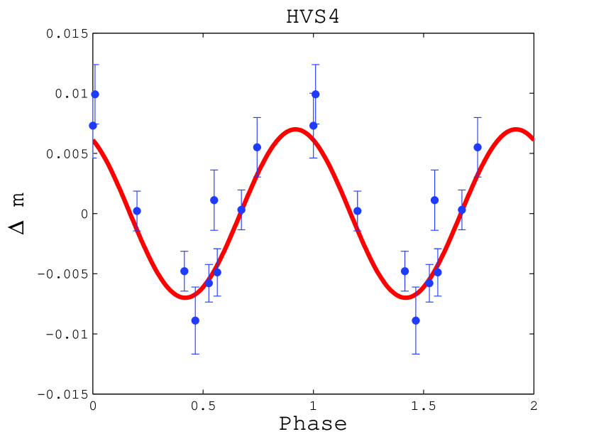
Figure 5.— Relative photometry of HVS4 as a function of phase angle. The light curve is folded according to the best-fit model with $P=0.18212$ days.

3.3. HVS5: An Ambiguous Object

HVS5 is the least constrained target. The variability suggests that HVS5 may be a SPB star, however our $F$-test gave a probability of 0.1225 which is significant to only 1.2-sigma. Therefore, we can not claim a detection for HVS5. Figure 6 shows our relative photometry for HVS5 and our periodogram. Our data from the Hiltner telescope correlated well with our data form the WIYN telescope, however the large errors ($\sim$ 2-3%) do not offer any additional constraints on the variability of HVS5, and are only shown for completeness. We find a best fit period of $P=0.53362\pm 0.00666$ days, with strong aliases at $P=0.337$ and 1.031 days. Our best fit amplitude is $A$ = 0.00538 $\pm 0.00031$ mag. Our $\chi^{2}_{min}$ = 39.0 for 9 degrees of freedom. Figure 7 shows our best fit model with our WIYN data folded about our best fit period. Further observations our necessary to help determine the nature of HVS5.

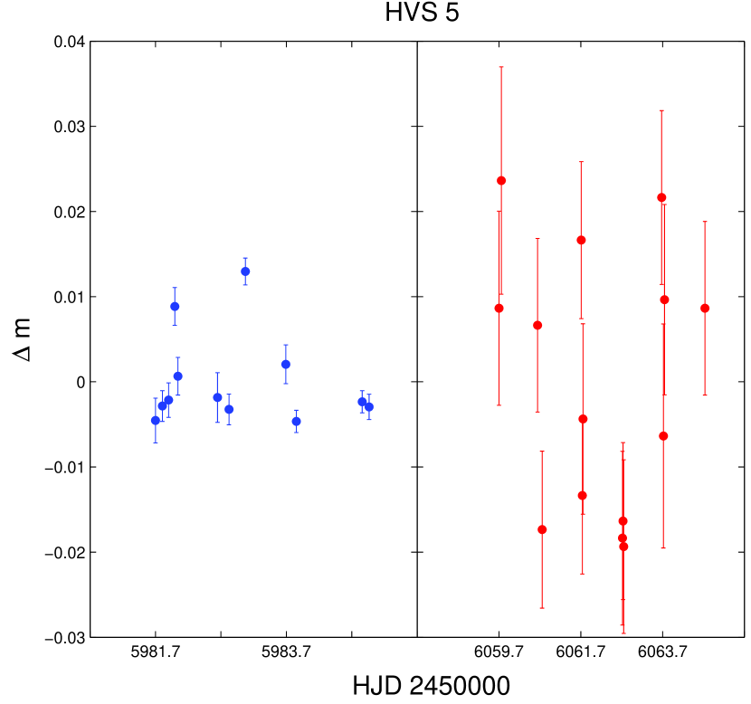
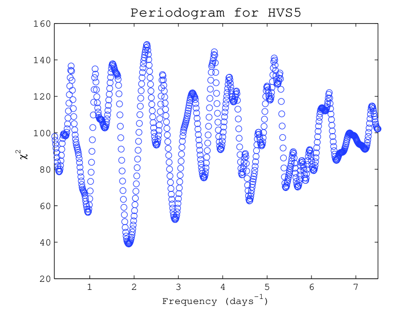
Figure 6.— Results for HVS5. Top: relative photometry of HVS5 with data taken from the WIYN 3.5 m (on the right) and the Hiltner 2.4 m telescope (on the left). For convenience the photometry was rescaled to have a mean of zero. This is $g$-band vs. HJD-2,450,000. Bottom: $\chi^{2}$ as a function of period (days). The best-fit model gives $P=0.53362\pm 0.00666$.

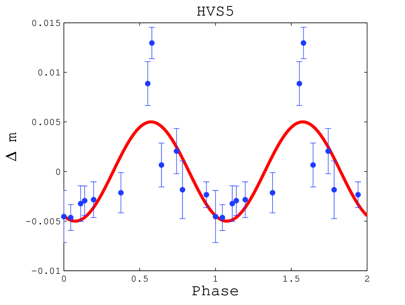
Figure 7.— Relative photometry of HVS5 as a function of phase angle. The light curve is folded according to the best-fit model with $P=0.53362$ days.

3.4. HVS7

HVS7 is our best constrained target. Our $F$-test gave a probability of 0.016 which has significance at the 2.5-sigma level. We find a best fit period $P=1.05261\pm 0.00194$ days, with a strong alias at $P=0.521$ days. Our best fit amplitude is $A$ = 0.02812 $\pm 0.00056$ mag. Our $\chi^{2}_{min}$ = 90.2 for 5 degrees of freedom. Figure 8 shows our relative photometry for HVS7 and our periodogram. Figure 9 shows our best fit model with our WIYN data folded about our best fit period. The data from the Hiltner telescope are shown for completeness.

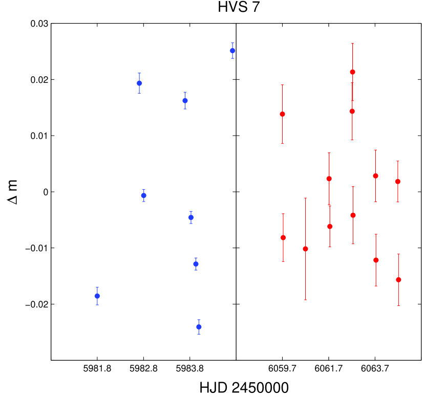
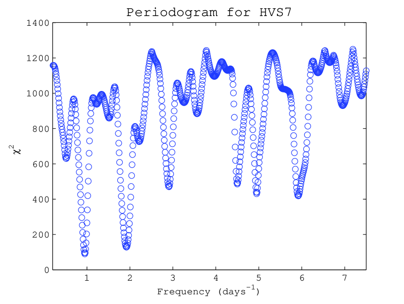
Figure 8.— Results for HVS7. Top: relative photometry of HVS7 with data taken from the WIYN 3.5 m (on the right) and the Hiltner 2.4 m telescope (on the left). For convenience the photometry was rescaled to have a mean of zero. This is $g$-band vs. HJD-2,450,000. Bottom: $\chi^{2}$ as a function of period (days). The best-fit model gives $P=1.05261\pm 0.00194$ days.

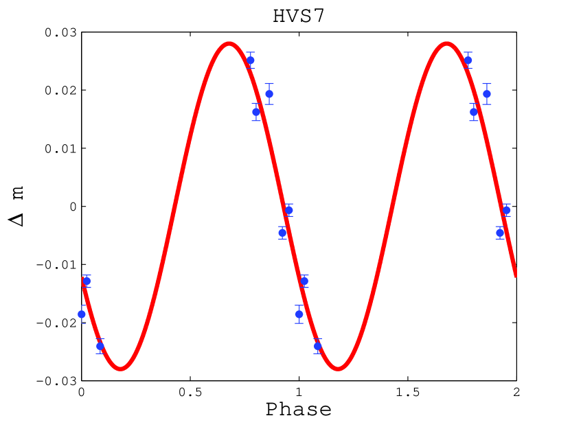
Figure 9.— Relative photometry of HVS7 as a function of phase angle. The light curve is folded according to the best-fit model with $P=1.05261$ days.

3.5. HVS13

HVS13 had the least amount of exposures, however our $F$-test gave a probability of 0.0283 which is significant to two-sigma. Our $\chi^{2}_{min}$ = 2.71 for 4 degrees of freedom, which is the best value for all five targets. We find the best fit period to be $P=0.38693\pm 0.00402$ days, with the strongest aliases at $P=2.000$ and 0.667 days. The best fit amplitude is $A$ = 0.02318 $\pm 0.00369$ mag. Figure 10 shows our relative photometry for HVS13 and our periodogram. Figure 11 shows our best fit model with our WIYN data folded about our best fit period.

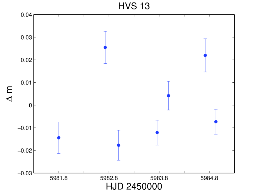
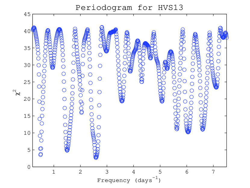
Figure 10.— Results for HVS13. Top: relative photometry of HVS13 with data taken from the WIYN 3.5 m telescope. For convenience the photometry was rescaled to have a mean of zero. This is $g$-band vs. HJD-2,450,000. Bottom: $\chi^{2}$ as a function of period (days). The best-fit model gives $P=0.38693\pm 0.00402$ days.

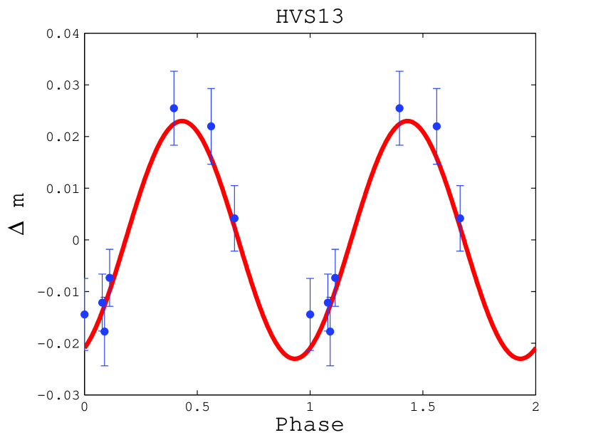
Figure 11.— Relative photometry of HVS13 as a function of phase angle. The light curve is folded according to the best-fit model with $P=0.38693$ days.

4. Summary and Conclusion

Table 2Summary of Results for each SPB Candidate

Star	RA	DEC	MB	NOAO	MDM	Period (days)	Amplitude (mag)	$\chi^{2}$	P(F-test)
HVS1	9:07:44.993	2:45:06.88	19.687	12	6	0.72738$\pm$0.00767	0.02878$\pm$0.00156	45.5	0.0825
HVS4	9:13:01.011	30:51:19.83	18.314	10	6	0.18212$\pm$0.00057	0.00672$\pm$0.00064	12.5	0.0463
HVS5	9:17:59.475	67:22:38.35	17.557	12	13	0.53362$\pm$0.00666	0.00538$\pm$0.00031	39.0	0.1225
HVS7	11:33:12.123	1:08:24.87	17.637	8	12	1.05261$\pm$0.00194	0.02812$\pm$0.00056	90.2	0.0160
HVS13	10:52:48.306	-0:01:33.940	20.018	7	6	0.38693$\pm$0.00402	0.02318$\pm$0.00369	2.71	0.0283

Note. — The leftmost column is the name of the HVS. The next two columns are the right ascension (RA) and declination (DEC) respectively, and following is the absolute magnitude (M). Next is the number of images taken with the WIYN 3.5 m telescope (NOAO) and the Hiltner 2.4 m telescope (MDM) respectively. The best fit period is given, followed by the amplitude, and $\chi^{2}$. The rightmost column is the value from the $F$-test.

We have taken time-series photometry of 11 HVSs (see Table 1) and determined that HVS1, HVS4, HVS7, and HVS13 show degrees of variability with best fit periods $\sim 0.2-1.0$ days and amplitudes $\sim 0.006-0.03$ mag. SPBs have observed periods between $0.5-4$ days which is consistent with our best fit periods. The variability of the target HVSs are a few millimagnitudes which again is consistent for SPBs. SPBs have masses $M_{\star}\sim 3-7$ M_⊙, and a number of confirmed SPBs (see De Cat & Aerts 2002) have mass $\sim 3$M_⊙ and T${}_{eff}\sim 12,000$ K which agrees with the spectroscopically derived masses and temperatures of HVS1, HVS5, HVS7, and HVS8 (Brown et al., 2012a). Our $F$-test shows that HVS1 is suspect, with only a 1.6-sigma detection. HVS4 and HVS13 both have a two-sigma detection, and HVS7 is detected at the 2.5-sigma level. HVS5 was constrained at only the 1.2-sigma level, and thus can not be considered a detection, however it warrants further investigation.

Within 200 pc of the GC are regions dominated by massive Wolf-Rayet and OB supergiants (Mauerhan et al. 2010; Dong et al. 2012). However, at the innermost 0.05 pc the S-stars, young B-stars with masses $\sim 7-15$ M_⊙ dominate (Ghez et al. 2003; Gillessen et al. 2009b). Ginsburg & Loeb (2006) suggested that the unexpected appearance of young stars around Sgr A* (Ghez et al., 2003) can be explained at least in part by Hill’s mechanism where a binary star is disrupted by the MBH resulting in the production of a HVS of one component, while the other star falls into a highly eccentric orbit around Sgr A*. Defining “arrival time” as the time between its formation and ejection (Brown et al., 2012a), we find that Hill’s mechanism provides an arrival time of $t_{arr}\sim 0.1-1$ Gyr (Merritt & Poon, 2004) which is consistent with the expected lifetime of a MS B star of $\sim 3$ M_⊙ . Furthermore, this scenario is supported by the results of $N$-body simulations (Ginsburg & Loeb 2007; Antonini et al. 2010). Recently, Bartko et al. (2010) found an isotropic distribution of B stars extending from the central arcsecond from Sgr A* to 12″. We identified four of 11 targets as as likely MS B stars. The fact that a significant percentage of our targets appear to be MS B stars helps support the case for an extended B star distribution.

To date, only five of the known HVSs have been studied with high-resolution spectroscopy. HVS2 (Hirsch et al., 2005) is believed to be a subluminous O star, while the other four are MS B stars. HVS1 is the only HVS that has been observed with time-series photometry before our observations, and our results agree with F06 that HVS1 is a SPB. However, F06 derived a period of $P\sim 0.35$ days while our most significant period alias is twice this value. HVS5 was recently observed with Keck HIRES spectroscopy (Brown et al., 2012a) which establishes it to be a MS B star, however our photometric data is ambiguous whether HVS5 may be a SPB star. Further observations will be necessary in order to confirm the nature of HVS5. HVS7 and HVS8 (López-Morales & Bonanos, 2008) are both believed to be MS B stars. Our results for HVS7 show it to be a SPB with $P\sim 1.0$ days. We did not detect a variability for HVS8. However, we can not rule out the possibility that it is a SPB with $P\geq 3$ days. The only other HVS with a detected variability was HVS13 with a period between $P\sim 0.4-2$ days, suggesting it is a SPB. Without further observations, the remaining HVSs are either: SPBs with $P\geq 3$ days, SPBs with amplitudes below 0.01 mag, MS B stars but non-SPBs, or BHB stars. Figure 12, from Degroote et al. 2009 summarizes our results in the context of the instability domain. The $x$-axis gives the period in days, and the $y$-axis denotes log of T_eff. Region $a$ shows the location of $\beta$ Cephei stars, which are early-type B stars (B0-B2.5) with variability of several hours (Stankov & Handler, 2005). $\delta$ Scuti stars, shown in region $c$, are of spectral type A and F with typical periods of 0.02-0.25 days (Breger, 2007). Region $d$ shows $\gamma$ Doradus variables with periods similar to SPBs, $\sim 0.3-3$ days, however they are of later spectral type A or F (Pollard, 2009). SPBs lie within region $b$. Currently, all known HVSs on the MS are B type stars and may be SPBs that lie within a small narrow strip of the instability domain illustrated by the black rectangle. However, further observations may support or modify the current paradigm.

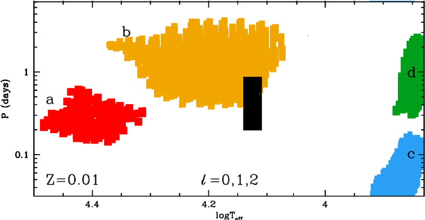
Figure 12.— Adapted from Degroote et al. (2009). The theoretical instability domains of $l$ = 0,1,2 modes are represented in a log $T_{eff}$ versus log $P$ diagram. The regions are as follows: $a$ = $\beta$ Cep, $b$ = SPB, $c$ = $\delta$ Sct, and $d$ = $\gamma$ Dor-type. These regions assume a metallicity Z = 0.01, however results vary little for higher metallicity. Our results fall in the narrow black strip as shown. We assume a $T_{eff}\sim$ 12,000 K.

References

- Antonini et al. (2010) Antonini, F., Faber, J., Gualandris, A., & Merritt, D. 2010, ApJ, 713, 90
- Antonini et al. (2011) Antonini, F., Lombardi, J., & Merritt, D. 2011, ApJ, 731, 128
- Bartko et al. (2010) Bartko, H., Martins, F., Trippe, S., et al. 2010, ApJ, 708, 834
- Bertin & Arnouts (1996) Bertin, E., & Arnouts, S. 1996, A&AS, 117, 393
- Bevington & Robinson (2003) Bevington, R., & Robinson, D. 2003, Data Reduction and Error Analysis for the Physical Sciences, 3rd edn. (Boston, MA: McGraw-Hill)
- Bonanos et al. (2008) Bonanos, A., López-Morales, M., Hunter, I., & Ryans, R. 2008, ApJ, 675, L77
- Breger (2007) Breger, M. 2007, CoAst, 150, 25
- Brown et al. (2010) Brown, W., Anderson, J., Gnedin, O., et al. 2010, ApJ, 719, L23
- Brown et al. (2012a) Brown, W., Cohen, J., Geller, M., & Kenyon, S. 2012a, ApJ, 754, 2
- Brown et al. (2009) Brown, W., Geller, M., & Kenyon, S. 2009, ApJ, 690, 1639
- Brown et al. (2012b) —. 2012b, ApJ, 751, 55
- Brown et al. (2005) Brown, W., Geller, M., Kenyon, S., & Kurtz, M. 2005, ApJ, 622, L33
- Brown et al. (2006a) —. 2006a, ApJ, 640, L35
- Brown et al. (2006b) —. 2006b, ApJ, 647, 303
- Brown et al. (2007) —. 2007, ApJ, 671, 1708
- Catelan (2009) Catelan, M. 2009, Ap&SS, 320, 261
- Contreras et al. (2005) Contreras, R., Catelan, M., Smith, H., Pritzl, B., & Borissova, J. 2005, ApJ, 623, L117
- De Cat & Aerts (2002) De Cat, P., & Aerts, C. 2002, A&A, 393, 965
- Degroote et al. (2009) Degroote, P., Aerts, C., Ollivier, M., et al. 2009, A&A, 506, 471
- Demarque & Virani (2007) Demarque, P., & Virani, S. 2007, A&A, 461, 651
- Dong et al. (2012) Dong, H., Wang, Q., & Morris, M. 2012, MNRAS, 425, 884
- Dziembowski et al. (1993) Dziembowski, W., Moskalik, P., & Pamyatnykh, A. 1993, MNRAS, 265, 588
- Edelmann et al. (2005) Edelmann, H., Napiwotzki, R., & Heber, H. 2005, ApJ, 634, L181
- Fuentes et al. (2006) Fuentes, C., Stanek, K., Gaudi, B., et al. 2006, ApJ, 636, 37, (F06)
- Gautschy & Saio (1995) Gautschy, A., & Saio, H. 1995, ARA&A, 33, 75
- Gautschy & Saio (1996) —. 1996, ARA&A, 34, 551
- Ghez et al. (2005) Ghez, A., Salim, S., Hornstein, S., et al. 2005, ApJ, 620, 744
- Ghez et al. (2003) Ghez, A., Duchêne, G., Matthews, K., et al. 2003, ApJ, 586, L127
- Ghez et al. (2008) Ghez, A., Salim, S., Weinberg, N., et al. 2008, ApJ, 689, 1044
- Gillessen et al. (2009a) Gillessen, S., Eisenhauer, F., Fritz, T., et al. 2009a, ApJ, 707, L114
- Gillessen et al. (2009b) Gillessen, S., Eisenhauer, F., Trippe, S., et al. 2009b, ApJ, 692, 1075
- Ginsburg & Loeb (2006) Ginsburg, I., & Loeb, A. 2006, MNRAS, 368, 221
- Ginsburg & Loeb (2007) —. 2007, MNRAS, 376, 492
- Ginsburg et al. (2012) Ginsburg, I., Loeb, A., & Wegner, G. 2012, MNRAS, 423, 948
- Ginsburg & Perets (2011) Ginsburg, I., & Perets, H. 2011, arXiv:1109.2284v1
- Gnedin et al. (2005) Gnedin, O., Gould, A., Miralda-Escudé, J., & Zenter, A. 2005, ApJ, 634, 344
- Hills (1988) Hills, J. 1988, Nature, 331, 687
- Hirsch et al. (2005) Hirsch, H., Heber, U., O’Toole, J., & Bresolin, F. 2005, A&A, 444, L61
- Jester et al. (2005) Jester, S., Schneider, D., Richards, G., et al. 2005, AJ, 130, 873
- Karaali et al. (2005) Karaali, S., Bilir, S., & Tunçel, A. 2005, PASA, 22, 24
- López-Morales & Bonanos (2008) López-Morales, M., & Bonanos, A. 2008, ApJ, 685, L47
- Mauerhan et al. (2010) Mauerhan, J., Cotera, A., Dong, H., et al. 2010, ApJ, 725, 188
- Merritt & Poon (2004) Merritt, P., & Poon, M. 2004, ApJ, 606, 788
- O’Leary & Loeb (2008) O’Leary, R., & Loeb, A. 2008, MNRAS, 383, 86
- Perets (2009a) Perets, H. 2009a, ApJ, 690, 795
- Perets (2009b) —. 2009b, ApJ, 698, 1330
- Pollard (2009) Pollard, K. 2009, AIPC, 1170, 455
- Przybilla et al. (2008a) Przybilla, N., Nieva, M., Heber, U., et al. 2008a, A&A, 480, L37
- Przybilla et al. (2008b) Przybilla, N., Nieva, M., Tillich, A., et al. 2008b, A&A, 488, L51
- Saha et al. (2000) Saha, A., Armandroff, T., Sawyer, D., & Corson, C. 2000, Proc. SPIE, 4008, 447
- Schödel et al. (2003) Schödel, R., Ott, T., Genzel, R., et al. 2003, ApJ, 596, 1015
- Sesana et al. (2009) Sesana, A., Madau, P., & Haardt, F. 2009, MNRAS, 392, L31
- Stankov & Handler (2005) Stankov, A., & Handler, G. 2005, ApJS, 158, 193
- Stetson (1987) Stetson, P. 1987, PASP, 99, 191
- Tody (1993) Tody, D. 1993, ASPC, 52, 173
- Turner et al. (2009) Turner, D., Kovtyukh, V., Majaess, D., & Moncrieff, K. 2009, AN, 330, 807
- Ushomirsky & Bildsten (1998) Ushomirsky, G., & Bildsten, L. 1998, ApJ, 497, L101
- Waelkens (1991) Waelkens, C. 1991, A&A, 246, 453
- Waelkens et al. (1998) Waelkens, C., Aerts, C., Kestens, E., Grenon, M., & Eyer, L. 1998, A&A, 330, 215
- York et al. (2000) York, D., Adelman, J., Andersen, J. J., et al. 2000, AJ, 120, 1579
- Yu & Tremaine (2003) Yu, Q., & Tremaine, S. 2003, ApJ, 599, 1129