Pulsar scintillations from corrugated reconnection sheets in the ISM

Abstract

We show that surface waves along interstellar current sheets closely aligned with the line of sight lead to pulsar scintillation properties consistent with those observed. This mechanism naturally produces the length and density scales of the ISM scattering lenses that are required to explain the magnitude and dynamical spectrum of the scintillations. In this picture, the parts of warm ionized interstellar medium that are responsible for the scintillations are relatively quiescent, with scintillation and scattering resulting from weak waves propagating along magnetic domain boundary current sheets, which are both expected from helicity conservation and have been observed in numerical simulations. The model statistically predicts the spacing and amplitudes of inverted parabolic arcs seen in Fourier-transformed dynamical spectra of strongly scintillating pulsars with only 3 parameters. Multi-frequency, multi-epoch low frequency VLBI observations can quantitatively test this picture. If successful, in addition to mapping the ISM, this may open the door to precise nanoarcsecond pulsar astrometry, distance measurements, and emission studies using these 10AU interferometers in the sky.

1 Introduction: observations and theoretical challenges

Compact radio sources provide a precision probe of the ionized interstellar medium (IISM). The propagation speed of radio waves depends on the density of free electrons, and therefore the spatial inhomogeneity of the IISM may result in refractive and diffractive abberation and scattering. This causes scintillation (time-variability) of the compact radio-sources (Scheuer, 1968; Blandford et al., 1986; Rickett et al., 2006). Observations of the pulsar scintillations are particularly interesting for infering the IISM properties, due to the brightness of many pulsars that have been observed for other purposes over long time intervals.

However, despite of considerable effort, the small-scale structure of the IISM has remained enigmatic. At a first glance, one expects the scattering to be caused by density inhomogeneities produced from turbulent motions of the IISM. However, this picture alone is unable to explain the last decade of the pulsar scintillation data. There, a major observational progress of the ISM scintillations has been achieved through the Stinebring et al. (2001) detection of inverted parabolic arc structures in the Fourier-transformed dynamical spectra of some strongly scintillating nearby pulsars at some epochs. These inverted parabolic arclets imply that for these pulsars the radio-wave scattering occurs mostly within one or a few thin screens (Walker et al., 2004; Cordes et al., 2006; Walker et al., 2008). Moreover, the multiple “inverted parabolae” (Hill et al., 2005) show that the scattering inside the screen is strongly inhomogeneous and occurs in localized clumps. The latter was recently confirmed by Brisken et al. (2010) who have constructed the scintillation derived scattering image of PSR B0834+06 from VLBI data. They have found that not only the scattering image was clumpy but that the clumps lined up along a thin line. Refractive effects are usually invoked to explain these phenomena (Cordes et al., 2006). The physical conditions to create these scattering angles are mysterious, and have been suggested to hint at new physical phenomena(Walker, 2007, 2001; Pérez-García et al., 2013). Goldreich & Sridhar (2006) showed that the interference of images in refractive lensing also results in scintillation which resembles purely diffractive processes.

We use the term “scattering” to refer to the general phenomenon of change of light propagation direction, for which one can consider different physical mechanisms, including diffraction and refraction.

In this paper, we explore the quantitative consequences of the refractive scintillation picture. Since refractive effects are required in any case, we explore the possibility if these alone can predictively explain the observations, and how this can be tested in the future. We study a scenario in which the scattering is produced by a refractive structure, with turbulence playing a secondary role. Radio-wave scattering by non-turbulent large-scale refractive structures has been previously considered by Romani et al. (1987), mostly in the context of the so-called extreme-scattering events observed by Fiedler et al. (1987). Recently, Goldreich & Sridhar (2006) proposed that the image of the SgrA* radio-source is strongly scattered by several reconnection sheets that are closely aligned with the line of sight to SgrA*. In this paper, we develop further the Goldreich & Sridhar’s (2006) idea [see also Pen & King (2012)] and apply it to construct a quantitative picture of pulsar scintillations. Namely, we consider a scenario where the pulsar radio-wave scattering occurs due to several weakly corrugated reconnection sheets that are closely aligned with the line of sight to the pulsar; see figure 1. We show that this scenario provides explanations for previously unexplained features of the scintillations: (1) the “scattering screens” are simply effective descriptions of such sheets; their location is marked approximately by the sheets’ intersections with the line of sight, (2) “the scattering clumps” correspond to those parts of sheet folds where the sheet is parallel to the line of sight; the strength of the scattering follows a strongly non-Gaussian distribution, even though the corrugation itself is assumed to be a realization of a Gaussian distribution, and (3) the strong non-isotropy of the Brisken et al. 2010 image is a consequence of the sheet’s inclination, with the clump locations aligned along the direction perpendicular to sheet’s line of nodes. The width of the image is given by the inclination angle of the sheet. (4) the high degree of alignment is a selection effect, as described by Goldreich & Sridhar (2006): all sheets aligned by less than the critical angle do not project into fold singularities (Whitney, 1955) and thus do not contribute to strong lensing. The plan of the paper is as follows: in the next section we briefly describe the origin of the reconnection sheets, in section 3 we derive the model for the fold statistics, in section 4 we derive the lensing by the corrugated sheet, and in section 5 we compute the Fourier-transformed dynamical spectrum and demonstrate the emergence of inverted parabolic arclets. In section 6 we discuss physical implications, section 7 future speculation, and conclude in section 8..

2 Astrophysical Picture

2.1 Two Regimes of Lensing: Diffractive vs Refractive

Two regimes to generate pulsar scintillation have been considered. Traditionally, scintillation has been treated as the scattering of radio waves by a volume filling random field, produced by a turbulent cascade (Rickett, 1990). This process produces structures on a large range of scales. In this paper, we will classify the lensing into two distinct regimes:

We define the diffractive limit of wave scattering when the angle is determined by the ratio of the wavelength $\lambda$ of the radio-waves, and the characteristic spatial scale $D$ of the scattering structure: $\theta\sim\lambda/D$. The brightness of the scattered image is determined by the amplitude of the wavefront modulation caused by the scattering structure. To explain the observed angles in the range $1-100$ mas at wavelength $\sim 1$m, requires structures in the ISM on transverse scales of order $10^{6-8}$m. This imposes unexpected properties on the IISM, since this scale much smaller than the coloumb mean free path of protons and thus compressive perturbations of this scale are overdamped and decay exponentially on the sound-crossing time-scale, which is hours to days. If one still assumes that somehow these perturbations are created and maintained, then the angular image of a pulsar, and therefore its dynamic spectrum, are superpositions of thousands of $\hbox{AU}/10^{8}\hbox{m}$ weak structures (for a 1-d scattering image), and are expected to be roughly Gaussian. The length scale is given by the path length difference, which in turn is inferred from the inverse scintillation correlation frequency. The asymmetric parabolically structured 2-D power spectrum of the dynamic spectrum containing inverted parabolic arcs, and the VLBI image of the scattering disk consisting of several prominent clumps, are inconsistent with such a picture. The number of $10^{6-8}$m eddies along the line of sight can be large, possibly $10^{13}$ for a pulsar at a distance of $\sim$ kpc. The total scattered power comes from the cumulative projected variation in refractive index, which grows as the square root of the number of eddies. Each eddie only needs to change the refractive index by a part in a million of the cumulative change, so a refractive index variation of a part in $\sim 10^{12}$ could account for the strong scintillation. But the superposition of scattering from such a large number of eddies would surely look very Gaussian by the central limit theorem. A requirement for the sum of $10^{13}$ contributions to appear intermittent in projection would lead to unphysically overpressurized eddies.

A second mechanism is due to refractive lensing. For structures larger than the Fresnel scale

$$r_{F}\equiv\sqrt{\lambda L}\sim 0.03AU\left(\frac{\lambda}{{\rm m}}\right)\left(\frac{L}{{\rm kpc}}\right)$$ (1)

deflection of light rays are described by geometric optics. In this regime, points of stationary phase in phase optics correspond to local extrema of Fermat’s principle, leading to multiple images of a source. The lens itself need not have structures on the diffractive scale, it is sufficient for the phase to linearly change by $2\pi$ on a scale $D=\lambda/\theta$. When all structures in the lens are larger than $r_{F}$, the refractive images will still show interference with each other, which resembles some of the properties of DISS. We will call this the refractive scintillation limit.

To further simplify this picture, we consider the bending angle as determined by Snell’s law, i.e. the change in refractive index and the angles of incidence. The refractive index of a plasma at frequency $\omega$ is $n=1/\sqrt{1-\omega_{p}^{2}/\omega^{2}}$, with plasma frequency $\omega_{\rm p}=\sqrt{n_{e}e^{2}/\epsilon_{0}m_{e}}$. Pulsar observations are done at frequencies much higher than the plasma frequency, for which we expand $n-1\sim-\frac{\omega_{p}^{2}}{2\omega^{2}}=-1.8\times 10^{-8}n_{e}$ at wavelengths of a meter. The observed scattered images at 20 mas require deflection angles of at least 40 mas, corresponding to $n_{e}\sim 10/{\rm cm}^{3}$ neglecting geometric alignment factors. However, the mean density of the IISM is determined to be of the order $10^{-2}$, as measured from the pulsars’ dispersion measure(Lorimer & Kramer, 2004). Therefore, the refractive picture is also challenging to reconcile with the data, since the observed scattering angles would naïvely require fractional changes in free electron density of $\sim 10^{3}$ which are difficult to understand or confine. This contraint, however, is alleviated when one considers refractive sheets that are closely aligned with the line of sight (Goldreich & Sridhar, 2006). At this grazing incidence, expressed as an angle $\alpha$ from the surface of the lens, the deflection angle is amplified to $\Delta\theta=n_{2}/n_{1}/\alpha$, so a sufficiently small $\alpha$ can result in a large deflection.

Historically, refractive lensing was used to interpret long time variability, and diffraction for the minute time scale effects. Recently, it was understood that the refractive images result in an interference fringe pattern (Walker et al., 2004) which have similar time and frequency scales for flux modulation as diffractive effects. The frequency and time scaling was historically interpreted as related to an underlying stochastic diffractive process driven by turbulence. Goldreich & Sridhar (2006) showed that refractive lensing by aligned sheets results in scintillation similar to the diffractive picture.

2.2 Physical origin of the reconnection sheets

The interstellar medium is stirred on scales of parsecs by various energetic processes, including supernovae, ionization fronts, spiral density waves, and other phenomena. These processes are generally short lived, and we conjecture after the stirring, the warm medium relaxes to an near-equilibrium configuration on small (several AU) scales. Current numerical simulations of the supernova-driven turbulence in the warm ISM of the Galaxy (e.g., Hill et al. 2011) do not have the resolution to tell how realistic this assumption is. In the presence of helicity, the equilibrium magnetic fields are configured as interlaced twisted tori, which are long lived (Braithwaite & Spruit, 2004). It has been shown by Gruzinov (2009) that a “generic magnetic equilibrium of an ideally conducting fluid contains a volume-filling set of singular current layers.” In this picture, the magnetic fields are locally almost parallel, with discontinuous interface regions, a bit like magnetic domains in a ferromagnet. Singular current sheets have also been seen in the simulations of Schekochihin et al. (2004).

At the boundary between between magnetic field configurations, current sheets maintain the discontinuities. Depending on the nature of reconnection, these current sheet may be self-enforcing due to inflow of fresh fields, maintaining a thickness potentially as thin as an electron gyromagnetic radius. At constant temperature, the pressure equilibrium in the direction perpendicular to the sheet implies that the electron density inside the sheet is enhanced by a factor $R$ given by

$$R-1\sim{B_{\rm out}^{2}-B_{\rm in}^{2}\over 4\pi P_{\rm out}},$$ (2)

where $B_{\rm in}$ and $B_{\rm out}$ is the magnetic field in and outside the sheet, and $P_{\rm out}$ is the non-magnetic pressure outside the sheet. The right-hand side of the above equation is thought to be of order $1$ for the IISM, but may be significantly larger if the IISM is magnetic-pressure dominated.

Depending on the ratio of heating time due to reconnection to cooling time, the thin sheet may have an enhanced temperature, in which case it can be underdense, with $R\rightarrow 0$ in the limit of a strong entropy injection.

Figure 1: lensing geometry. The earth is at left, pulsar at right. A section of the (crumpled) scattering sheet is shown in the middle as the solid line. It may be a plasma under- or overdensity of constant thickness. The dashed line shows the unperturbed light path. The dotted line shows the path of an image lensed by a fold singularity of the projected sheet. The long dashed line shows the position of the sheet in the absence of waves. The inclination between this sheet and the line of sight is $\alpha$, in this plot 1/8, chosen to exagerate the effect for visual clarity, and reduce the computational cost. In practice, we envision values closer to $10^{-3}$.

The lensing geometry is shown in Figure 1. A crucial ingredient in our model is that the reconnection sheet is assumed to be weakly corrugated. Let us assume that the corrugation pattern is fixed, and vary the inclination angle. In this case, as can be seen from figure 1, there is characteristic inclination angle $\alpha$ at which the perturbations in the sheet can generate fold singularities in the projected surface density. This angle $\alpha$ is the ratio of the wave peak displacement to its wavelength. We envision ranges of $\alpha\sim 10^{-3}-10^{-2}$. When the fold singularities are present, they become effective refractive scattering centers for the radio waves. The resulting lense features multiple images that closely line up along the direction perpendicular to the line of nodes of the scattering sheet.

2.3 Surface Dynamics

We assume that the current sheet is physically thin, $\mathrel{\hbox{\hbox to0.0pt{\hbox{\lower 4.0pt\hbox{$\sim$}}\hss}\hbox{$<$}}}$ AU. Theoretically, the thickness of current sheets is not understood, so we choose this scale to be thin enough to explain the smallest scale observed structures. On each side the magnetic field points in a different direction. The change in Alvénic properties gives rise to surface waves (Jain & Roberts, 1991; Joarder et al., 2009), whose amplitude decays exponentially with the distance to the current sheet and which are mathematically analogous to deep water ocean waves. The restoring force is due to the difference in magnetic field component projected along the wave vector. Like ocean waves, these waves penetrate about a wavelength into each side. We will be considering wavelengths of hundreds to thousands of AU whose projected wavelength is related to the observed lensing structures $\sim$several AU, so the thickness of the current sheet itself is neglible as far as the dynamics of the waves are concerned. Seen in projection along the aligned sheet, the projected wavelengths will be $\sim$ AU, reduced by the alignment angle $\alpha$.

The displacements are transverse to the wave vector, and perpendicular to the sheet. While Alvénic in nature, the surface modes possess only one polarization, unlike bulk waves. We speculate such modes to be long lived, since the single polarization nature protects them from the normal MHD turbulent cascade(Goldreich & Sridhar, 1997). These waves resemble a flag blowing in the wind. Disturbances travelling along the sheet are decoupled from bulk waves. Being confined to a sheet, the amplitude away from a source drops as $\propto 1/r$ instead of the normal inverse square law. The 2-D analogy to Olber’s Paradox leads to flux being dominated by the cumulative effect of far away sources, like waves on an ocean beach. We speculate potential sources to include shock waves, spiral arms, stellar perturbations. A amplitude of order $\alpha\lambda_{\rm wave}$, or about $10^{-3}$–$10^{-2}$ of the wavelength of the surface wave, is sufficient to cause the sheet to appear folded in projection; here $\lambda_{\rm wave}$ is the wavelength of the surface wave.

3 Fold Statistics

We expect a minimum wavelength of these surface waves, which is substantially larger than the thickness of the sheet. Short wavelength perturbations are not bound to the surface, and can dissipate into the bulk. The exact cutoff depends on unknown factors, including the distance to the source, and vertical structure of the current sheet. Non-linear effects also cause short wavelength waves to dissipate, just like sound waves in the air. Primarily waves with amplitude larger than $\alpha$ contribute to scattering. The strength of damping depends on the distance to the source in units of wavelength, with shorter wavelengths being more damped.

We model the waves as a displacement function $\zeta(x)$ which is a Gaussian random field with a correlation function that is a Gaussian,

$$\xi(r)=\langle\zeta(x)\zeta(x+r)\rangle=A^{2}\exp\left(-{r^{2}\over 2\sigma^{2}}\right),$$ (3)

where $A$ is the mean amplitude of the displacement and $\sigma$ is the surface-wave coherence scale. The coordinates are as denoted in Figure 1: $x$ is the along the line of sight, which is closely aligned to the long axis along the sheet, and we use the same label for both. $y$ refers to the position as seen on the sky. We denote the projected coherence scale $\sigma_{y}\equiv\alpha\sigma$. Figure 2 shows a realization of a sheet with a random fluctuations. The displacement $\zeta$ is measured perpendicular to the sheet, and thus neither $x$ nor $y$. Since we are considering highly inclined sheets, $\zeta\sim y$ to within $\alpha$, and we will use these two interchangably. To reduce the computational cost, we used an inclination slope $\alpha=1/8$ instead of the physical range $\alpha\sim 10^{-3}-10^{-2}$, and a correlation length along the sheet of 350 units, which is $\sigma_{y}\sim 44$ grid units in projection. The displacement amplitude is chosen as $A=40$. The dimensionless fluctuation $\delta\equiv A/\sigma\sim 1$ is about unity, meaning a $1-\sigma$ fluctuation can result in a fold singularity, which we will discuss further below.

Figure 2: Sheet with transverse perturbations. The upper panel shows an zoomed version of a short section. The $x$ axis is along the line of sight, the $y$ axis is transverse. In a physical setting, the grid units roughly map to A.U. for the $x-axis$, and deci A.U. for the $y-axis$. The difference in conversion comes from the order of magnitude smaller inclination in the real system from the picture shown.

The current sheet corresponds to a change in magnetic and thermal pressure and thus has a refractive index different from the ambient ISM. For Alvénic waves, we can treat the sheet as constant thickness, and consider its convergence as is relevant for refractive lensing. In projection along the line of sight, the column density of the sheet results in a highly non-Gaussian distribution. Figure 3 shows the column density distribution in a simulation. Folds occur when the gradient of the displacement is equal to $-\alpha$, which as described above is quantified by the fluctuation amplitude $\delta$. The value chosen here makes folds common, occuring roughly once per correlation length, and yet make multiple folds overlapping in projection rare. Each fold results in two fold singularities, with characteric separation $\sigma_{y}$. This is well understood from the theory of extrema of surface waves(Longuet-Higgins, 1957).

Figure 3: projected density. The upper panel is a zoom of the central portion of the lower panel. Each time the sheet folds in projection, we see a double peaked structure in density. The characteristic separation between the two peaks is a projection correlation length $\sigma_{y}$, in this case 44 grid units.

Equation (5) describes the 1 point PDF corresponding to the spatial density distribution shown in figure 3. The deflection angle is determined by the gradient of the density, $\rho^{\prime}$.

As in Pen & King (2012), we use the notation of gravitational lensing(Schneider et al., 1992). The phase delay through the lens is described by the lensing potential

$$\psi\equiv\frac{\Delta z\omega_{p}^{2}}{2L\omega^{2}}$$ (4)

where $\Delta z$ is the thickness of the sheet along the line of sight. $L$ is the distance to the pulsar. The convergence $\kappa\equiv\partial_{\theta}^{2}\psi/2$ is given by the second angular derivative of the potential, and thereby the laplacian of the projected density $\rho$. The magnification gives the brightness of the image. In 1-D it is $\mu=1/(1-2\kappa)$, derived from the determinant of the amplification matrix. A negative amplification corresponds to a flipped image of odd parity.

As before, $\alpha$ is the angle between the screen and the line of sight. Then the convergence is $\kappa\propto 1/\alpha$ for $\alpha\ll 1$, and $P_{\rm screen}(\kappa)\propto 1/\kappa^{2}$, where $P_{screen}(\kappa)$ is the probability of a piece of screen to have convergence of $\kappa$. However, we are interested in the probability density with respect to the impact parameter relative to the line of sight, and not with respect to the location on the screen. For nearly aligned screens, this is not the same thing. In particular, part of the screen with low $\alpha$ occupies less of the impact-parameter space than the part of the screen with the same area but high $\alpha$. Thus,

$$P_{\rm impactparameter}(\rho)\propto 1/\rho^{3}$$ (5)

which is a strongly non-Gaussian distribution.

The regions near the locations where the screen is parallel to the line-of-sight, called fold singularities, give rise to the localized clumps in the pulsar’s scattering image, which produce the inverted parabolic arcs in pulsar secondary spectra.

4 Lensing

The lensing of this density sheet can be computed in analogy to Pen & King (2012); Clegg et al. (1998).

Figure 4: deflection angle mapping. The horizontal axis is angle on the sky, and the vertical axis is the intersection of this light ray on the source plane. Whenever multiple different directions on the sky intersect on the same position in the source plane, multiple images are formed, which form a coherent interference pattern. As before, the upper panel is a zoom of the lower panel.

Given the projected column density distribution in Figure 3, and assuming that the sheet has a fixed thickness along its normal, we can compute the mapping of apparent angle on the sky to position in the source (pulsar) plane. The fold singularities in the projected density distribution lead to large angle deflections, and multiple images, whenever the sheets are aligned closely enough for the folds to form. This explains why only a small fraction of the current sheets contribute to scintillation.

The system depends on the three dimensionless parameters: the projected perturbation amplitude $\delta$, the ratio $r$ of sheet thickness $z$ to the projected correlation length $\sigma_{y}$, and the characteristic overdensity $C$ at a fold singularity, described in more detail below.. The model predicts the number density of images and their fluxes as a function of their angular separation from the line of sight (and therefore as the function of time lag).

There is a dimensional scaling of time units, which is a function of pulsar transverse velocity, projected screen size, and observing frequency. This is generally parameterized as the DISS time scale, $t_{\rm DISS}\sim(\lambda/D)(L/v)$ where $D$ is the size of the lensing region, $L$ is the distance to the pulsar, $\lambda$ is the observing wavelength, and $v$ is the pulsar transverse velocity. Note that in this model, the lensing is refractive, sharing the time scales from diffractive models, but not the length scales.

We show a histogram of image magnifications in Figure 5, which can be compared to holographic flux measurements (Walker et al., 2008). The lensed images correspond to the inverted arclets seen in secondary spectra. The model predicts the number of images as a function of separation, shown in figure 6.

Figure 5: PDF of image magnifications. The peak near 1 are images at the unscattered positions, while the population on the left are lensed images. The peak occurs at roughly $1/\kappa$.

The separation of images is related to the separation of folds. For the majority of our simulation $\delta\sim 1$, and the separation is given by the projection correlation length $\sigma_{y}$. For $\delta\ll 1$, the angular density of folds becomes very rare, proportionate to an error function.

Figure 6: PDF of image positions per logarithmic distance interval on the sky $y$. The projected correlation length is $\sigma_{y}\sim 44$. The characteristic convergence $\kappa\sim 20$, leading to a cutoff near $\sigma_{y}\kappa\sim 1000$.

The number of images is determined by the number of light folds along the line of sight, i.e. how often the deflection angle is larger than the separation to the line of sight in Figure 4. Each projected fold results in two fold singularities and thus four images.

Figure 7: Average Spatial Distribution of flux per logarithmic distance interval. In a Gaussian model, the flux per image drops as $1/\theta$.

The maximum deflection angle of an image is the change of refractive index in the sheet, amplified by the alignment angle on a fold singularity. For a sheet much thinner than the projected fluctation amplitude, the maximum projected density enhancement $C\equiv\rho/\bar{\rho}$ relative to the projected mean sheet density $\bar{\rho}\sim n_{e}\Delta z/\alpha$ at a fold singularity is the square root of the radius of curvature to the thickness of the sheet $\tau$, $C=\sigma_{y}/\sqrt{A\tau}$ in the limit $\sigma^{2}/A\gg\tau$.

5 Simulated Dynamic Spectra

With the density field, we can solve the lens equations to simulate dynamic spectra. By adding the voltage field from each image with their appropriate amplitude and phases, we simulate the dynamic spectrum, shown in figure 8.

       

Figure 8: dynamic pulsar spectrum. Left panel is the simulated spectrum. Right panel is the dynamic spectrum of PSR B0834+06 from the Brisken et al (2010) dataset. Horizontal axis is time, vertical axis is frequency. For B0834, the horizontal axis is 4 MHz of bandwidth and the vertical axis 1.5 hours of time. We reproduce the characteristic criss-cross pattern observed in real scintillation spectra.

A 2-D fourier transform maps this dynamic spectrum into a secondary spectrum, shown in figure 9.

      

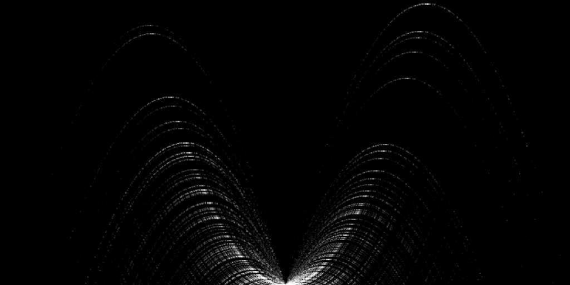
Figure 9: simulated model secondary pulsar spectrum. The inverted parabolic arcs at large delay arise naturally in this model from the interference of the distant lensed images at the apparent sheet fold singularity with the brighter, closer in images. The axis scales are meant to be illustrative, and depend on distance, pulsar velocity, etc

We find that the interference of these discrete, co-linear images forms the inverted parabolic arcs, qualitatively similar to those that are observed in Stinebring et al. (2001) and Hill et al. (2005).

6 Discussion

We can estimate the length scales involved in making the current sheet that would produce the observed scintillation pattern. This theory requires as input a current sheet thickness, inclination angle, curvature, amplitude of waves, and dissipation scale.

The thickness of the sheets can be estimated by considering the magnification of images. As shown in Pen & King (2012), the flux is roughly the thickness divided by the impact parameter. This follows from flux conservation of lensing: the net flux is conserved, and flux changes by order unity at impact parameters of order the physical size of the lens, so the typical flux off-axis is roughly the ratio of the furthest distance at which at image forms, to the size the lens.

The projected wavelengths are observed to be of order $\sim 10$ AU; this suggests a typical thickness of $h\mathrel{\hbox{\hbox to0.0pt{\hbox{\lower 4.0pt\hbox{$\sim$}}\hss}\hbox{$<$}}}0.1$AU to explain the $\sim$ 1% scattering intensities observed in Brisken et al. (2010).

The largest observed deflection angles at meter wavelength are $\gamma\sim 0.01$”, which requires an electron density change $\delta n_{e}\sim 100\alpha/C$ cm^-3. For a typical interstellar plasma density of $n_{e}\sim 0.03$ determined from pulsar dispersion, we need an alignment of a fraction of a degree, with fluctuation amplitude $C\sim 30$ and a wavelength of $\lambda\sim 1000$ AU. This combination is not unique.

As discussed in Pen & King (2012), the phenomenology of the Extreme Scattering Events prefers underdense lenses. In an underdense sheet, the maximal change of density is the density itself. With the assumption $\delta n_{e}\sim n_{e}$, we obtain $\alpha\sim 10^{-2}$. The probability of seeing a sheet at such an angle is $\sim\alpha^{2}$, requiring the existence of $\sim 1/\alpha^{2}$ sheets along the line of sight: if we imagine each “sheet” to be a thin disk, the probability of seeing a disk at angle $\alpha$ gets one contribution from the intrinsic alignment distribution, and one more from the reduced geometric cross section of an aligned sheet.

For pulsar B0834+06, the distance is $\sim 0.64$ kpc (as determined from the Dispersion Measure, and consistent with VLBI and ISM geometries(Brisken et al., 2010), also direct parallax: Deller and Brisken, unpublished ), giving a typical sheet separation of $s\sim 0.1$ pc.

These estimates are qualitative. One expects current sheets to come in a range of sizes, curvature and perturbation amplitude. The thickness might also vary.

One of the attractive features of our mechanism is that it explains very naturally the 1-d image of Brisken et al. (2010). The reduced dimensionality of the scattering image comes from the fact that the deflection created by the screen is mostly in the direction perpendicular to the screen’s line of nodes. Therefore, the scattering clumps will also form a line that is perpendicular to the line of nodes. This is demonstrated in Fig. 10, where we show a simulated 2-d scattering image of a pulsar. The alignment of the scattering clumps is apparent.

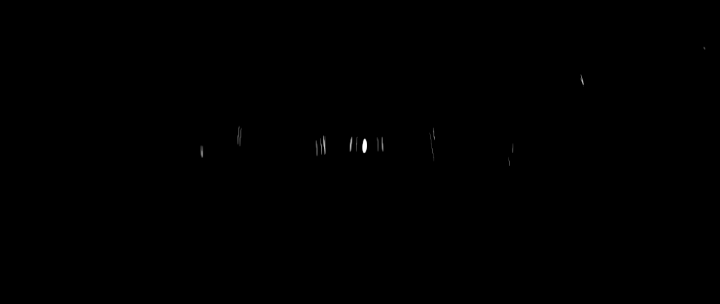
Figure 10: Simulated scattering image of the pulsar. A typical scale for this image would be 100 mas end-to-end. The pulsar is modeled as a unit disk, with a much exagerated diameter of 2 mas. The actual size of the pulsar emission spot would be $\sim 100$ picoarcseconds. Flux conservation requires that the sum of image areas equals the original disk. Thus, each pixel is either white or black in this figure. This compares favourably with the VLBI reconstructed positions of Brisken et al. (2010), where Fig 5 also shows images closely aligned along a straight line.

7 Future Potential

In our picture, pulsar scintillation is dominated by a small number of magnetic discontinuities highly aligned to the line of sight. Surface waves will move very slowly in this projected geometry, allowing for a precise determination of the geometric properties. This allows the use of these sheets as lenses to study both pulsars and the ISM(Pen et al., 2014). It could also have application to Intra-day variables(Macquart & de Bruyn, 2006) and the hyperstrong scattering at the galactic center.

7.1 ISM dynamics

Free parameters in our model include the thickness of the sheet and the inclination angle. These can be inferred by broad band measurements of pulsar scintillation, as follows. Firstly, the apparent position of images is expected to shift by a distance of order of the sheet width, as one decreases the observing frequency from the highest critical frequency at which the image forms, to a factor of two below(Pen & King, 2012). Secondly, the co-linearity of the images is related to the inclination angle of the sheet: the more aligned is the sheet with the line of sight, the greater is the aspect ratio of the scattering image.

7.2 Pulsar Emission imaging

A straightforward application is the study of the reflex motion of the emission region of the pulsar across the pulse phase. One expects the apparent emission region to move by distance of order of the effective emission height multiplied by the ratio of the pulse width to the rotation period. Using VLBI mapping of the scattering geometry, one can precisely predict the change of scintillation pattern as a function of pulse phase. The effective astrometric precision can be sub nano arcsecond(Pen et al., 2014).

7.3 Distance Measurement

It is tempting to use these lenses to obtain precision parallax distances to pulsars. It is difficult to keep the lens stable over a year, when typical pulsars move by much more than an astronomical unit, making the differential measurements challenging. For pulsars in binary systems, as is typical in millisecond pulsars, the orbital motion about its companion will modulate the scintillation pattern. This can be used to solve for the precision distance to the pulsar.

In the sheet lensing scenario, one can imagine obtaining widely separated scattering images: the lensing angle scales as $\propto\lambda^{2}$, so at low frequencies, for example with the LOFAR LBA, hundreds of AU are probed.

This could result in direct parallax distances with nano arc second precision, enough to determine pulsar distances for coherent gravitational wave detection (Boyle & Pen, 2012).

8 Conclusions

We have presented a quantitative theory of pulsar scintillation inverse parabolic arcs. These extend recent ideas of Goldreich & Sridhar (2006) and Pen & King (2012) about thin current sheets as the scattering objects in the ISM, which naturally explain the large angle scattering observed in pulsars and some extragalactic sources.

This picture could explain all scintillation phenomena from refractive lensing, all with structures greater than 0.1 AU. The apparent diffractive structure results from the interference between refractive images, and no diffractive scattering is needed.

In this scenario, VLBI monitoring of pulsars on time scales of weeks, at multiple low frequencies, can allow forecasts of the scattering behaviour. This in turn could improve gravitational wave timing residuals. The same scenario also enables the coherent use of the scattered images as a gigantic interstellar interferometer to map the motions of the pulsar emission regions.

9 Acknowledgements

U-LP thanks NSERC and CAASTRO for support. YL is supported by the Australian Research Counsil Future Fellowship.

References

- Blandford et al. (1986) Blandford R., Narayan R., Romani R. W., 1986, ApJ, 301, L53
- Boyle & Pen (2012) Boyle L., Pen U.-L., 2012, Phys. Rev. D , 86, 124028
- Braithwaite & Spruit (2004) Braithwaite J., Spruit H. C., 2004, Nat, 431, 819
- Brisken et al. (2010) Brisken W. F., Macquart J.-P., Gao J. J., Rickett B. J., Coles W. A., Deller A. T., Tingay S. J., West C. J., 2010, ApJ, 708, 232
- Clegg et al. (1998) Clegg A. W., Fey A. L., Lazio T. J. W., 1998, ApJ, 496, 253
- Cordes et al. (2006) Cordes J. M., Rickett B. J., Stinebring D. R., Coles W. A., 2006, ApJ, 637, 346
- Fiedler et al. (1987) Fiedler R. L., Dennison B., Johnston K. J., Hewish A., 1987, Nat, 326, 675
- Goldreich & Sridhar (1997) Goldreich P., Sridhar S., 1997, ApJ, 485, 680
- Goldreich & Sridhar (2006) Goldreich P., Sridhar S., 2006, ApJ, 640, L159
- Gruzinov (2009) Gruzinov A., 2009, ArXiv e-prints 0909.1815
- Hill et al. (2005) Hill A. S., Stinebring D. R., Asplund C. T., Berwick D. E., Everett W. B., Hinkel N. R., 2005, ApJ, 619, L171
- Jain & Roberts (1991) Jain R., Roberts B., 1991, Solar Physics, 133, 263
- Joarder et al. (2009) Joarder P. S., Ghosh S. K., Poria S., 2009, Geophysical and Astrophysical Fluid Dynamics, 103, 89
- Longuet-Higgins (1957) Longuet-Higgins M. S., 1957, Royal Society of London Philosophical Transactions Series A, 249, 321
- Lorimer & Kramer (2004) Lorimer D. R., Kramer M., 2004, Handbook of Pulsar Astronomy
- Macquart & de Bruyn (2006) Macquart J.-P., de Bruyn A. G., 2006, A&A, 446, 185
- Pen & King (2012) Pen U.-L., King L., 2012, MNRAS, 421, L132
- Pen et al. (2014) Pen U.-L., Macquart J. P., Deller A., Brisken W., 2014, MNRAS, in press
- Pérez-García et al. (2013) Pérez-García M. Á., Silk J., Pen U.-L., 2013, Physics Letters B, 727, 357
- Rickett (1990) Rickett B. J., 1990, ARA&A, 28, 561
- Rickett et al. (2006) Rickett B. J., Lazio T. J. W., Ghigo F. D., 2006, ApJS, 165, 439
- Romani et al. (1987) Romani R. W., Blandford R. D., Cordes J. M., 1987, Nat, 328, 324
- Schekochihin et al. (2004) Schekochihin A. A., Cowley S. C., Taylor S. F., Hammett G. W., Maron J. L., McWilliams J. C., 2004, Physical Review Letters, 92, 084504
- Scheuer (1968) Scheuer P. A. G., 1968, Nat, 218, 920
- Schneider et al. (1992) Schneider P., Ehlers J., Falco E. E., 1992, Gravitational Lenses
- Stinebring et al. (2001) Stinebring D. R., McLaughlin M. A., Cordes J. M., Becker K. M., Goodman J. E. E., Kramer M. A., Sheckard J. L., Smith C. T., 2001, ApJ, 549, L97
- Walker (2001) Walker M. A., 2001, Ap&SS, 278, 149
- Walker (2007) Walker M. A., 2007, in Haverkorn M., Goss W. M., eds, SINS - Small Ionized and Neutral Structures in the Diffuse Interstellar Medium Vol. 365 of Astronomical Society of the Pacific Conference Series, Extreme Scattering Events: Insights into the Interstellar Medium on AU-Scales. p. 299
- Walker et al. (2008) Walker M. A., Koopmans L. V. E., Stinebring D. R., van Straten W., 2008, MNRAS, 388, 1214
- Walker et al. (2004) Walker M. A., Melrose D. B., Stinebring D. R., Zhang C. M., 2004, MNRAS, 354, 43
- Whitney (1955) Whitney H., 1955, The Annals of Mathematics, 62, 374