Efficient computation of steady solitary gravity waves

Abstract.

An efficient numerical method to compute solitary wave solutions to the free surface Euler equations is reported. It is based on the conformal mapping technique combined with an efficient Fourier pseudo-spectral method. The resulting nonlinear equation is solved via the Petviashvili iterative scheme. The computational results are compared to some existing approaches, such as Tanaka’s method and Fenton’s high-order asymptotic expansion. Several important integral quantities are computed for a large range of amplitudes. The integral representation of the velocity and acceleration fields in the bulk of the fluid is also provided.

Key words and phrases: Surface waves; gravity waves; Euler equations; solitary wave; Petviashvili method

1.  Introduction

Solitary waves play a central role in nonlinear sciences [53]. They appear in various fields ranging from plasmas physics [46] to hydrodynamics [39] and nonlinear optics [33]. For integrable models, it can be rigorously shown that any smooth and localised initial condition will split into a finite number of solitons plus a radiation [65]. Solitons are special solitary waves interacting elastically, i.e., subject only to phase shifts after collisions [23, 65]. However, in full Euler equations, the interaction is known to be inelastic [57]. In some sense, solitons are elementary structures which span the system dynamics [51] along with (relative) equilibria [54], periodic orbits [18], etc. This is one of the main reasons why these solutions attract so much attention.

In some special cases the solitary waves can be found analytically. For example, explicit expressions are known for integrable models such as KdV and NLS equations [31, 32, 66], but also for some non-integrable Boussinesq-type [2, 3, 22] and Serre–Green–Naghdi [20, 24, 35, 58] equations. The examples of such analytical solutions are numerous [48]. However, no closed-form solutions are known for the practically very important case of the free surface Euler equations. Craig & Sternberg (1988) showed that solitary wave solutions to the Euler equations are necessarily positive and symmetric [16] (without surface tension effects). In order to construct these solutions, one has to apply some approximate methods. Historically, high-order asymptotic approximations have been proposed first [27, 43]. However, these solutions are asymptotic by construction and are therefore valid only in the limit $a/d\to 0$ ($a$ being the wave amplitude, $d$ the uniform undisturbed water depth); moreover, these series are known to be divergent [34]. In order to avoid this limitation, several numerical approaches have been proposed [28, 52] such as the Dirichlet-to-Neumann operator method [15] or Boundary Integral Equation method [63]. High amplitude solitary waves up to the limiting wave were studied by Longuet-Higgins & Tanaka [45], among others. One of the most widely used methods nowadays is the Tanaka algorithm [60]. In the present study, we are going to compare extensively our computational results to Tanaka’s method.

The approach we proposed in a short recent preliminary study [10] is also based on the conformal mapping technique, as the Tanaka method [60], for example. However, traditionally the conformal map is coupled with the Newton method [37] to find the solitary wave profil [4, 42, 50]. Newton-type iterations require the computation of a Jacobian matrix and the resolution of linear systems of equations (by direct or iterative methods) [62]. From a computational point of view, simple iterative schemes are much easier to implement and they require only the evaluation of operators involved in the equation to be solved. In the previous study [10], we adopted the classical Petviashvili’s iteration [56] in which the convergence is ensured by computing the so-called stabilising factor [55]. This iterative scheme have been already applied to compute special solutions to many nonlinear wave equations [40, 64, 25, 26]. An interesting comparison among different methods was recently performed for the solitary waves to the Benjamin equation [21]. The combination of two main ingredients, i.e., the Petviashvili scheme together with the conformal mapping technique, allowed us to propose a very efficient numerical scheme for the computation of solitary gravity waves of the full Euler equations in the water of finite depth [10]. The proposed algorithm admits a very compact and elegant implementation in Matlab, for example. The resulting script is ready to use and it can be freely downloaded from the Matlab Central server [8].

In the present study we perform further tests and validations of the new algorithm. Moreover, several important integral characteristics such as the mass, momentum, energy, etc. are derived in the conformal space and computed numerically to the high accuracy for a wide range of solitary waves. Our method allows also to compute efficiently important physical fields in any point inside the bulk of the fluid layer. In this way, the pressure, velocities and accelerations are shown under a large amplitude solitary wave, up to an arbitrarily high accuracy.

This study is organised as follows. In Section 2 we present the governing equations along with the conformal map technique. Several important integral quantities expressed in the transformed space are provided in Section 2.2. The Babenko integral equation is derived in Section 2.3. The following Section 3 contains the description of the numerical scheme along with some validations and tests. Finally, some conclusions of this study are outlined in Section 4.

2.  Mathematical model

Figure 1. Definition sketch of the physical and transformed domains.

We consider steady two-dimensional potential flows due to surface gravity solitary waves in constant depth. The fluid is homogeneous, the pressure is zero at the impermeable free surface and the seabed is fixed, horizontal and impermeable.

Let be $(x,y)$ a Cartesian coordinate system moving with the wave, $x$ being the horizontal coordinate and $y$ the upward vertical one. Since solitary waves are localised in space, the surface elevation tends to zero, along with all derivatives, as $x\to\pm\infty$, and $x=0$ is the abscissa of the crest. The equations of the bottom, of the free surface and of the mean water level are given correspondingly by $y=-0pt$, $y=\eta(x)$ and $y=0$. The parameter $a\equiv\eta(0)$ denotes the wave amplitude. Since gravity solitary waves of the Euler equations are known to be symmetric and positive [16], we have $\eta(-x)=\eta(x)\geqslant 0$ and $a=\max(\eta)$.

Let be $\phi$, $\psi$, $u$ and $v$ the velocity potential, the stream function, the horizontal and vertical velocities, respectively, such that $u=\phi_{x}=\psi_{y}$ and $v=\phi_{y}=-\psi_{x}$. It is convenient to introduce the complex potential $f\equiv\phi+\mathrm{i}\/\psi$ (with $\mathrm{i}^{2}=-1$) and the complex velocity $w\equiv u-\mathrm{i}\/v$ that are holomorphic functions of $z\equiv x+\mathrm{i}\/y$ (i.e., $w=\mathrm{d}f/\mathrm{d}z$). The complex conjugate is denoted with a star (e.g., $z^{\ast}=x-\mathrm{i}\/y$), while subscripts ‘b’ denote the quantities written at the seabed — e.g., ${z}_{\text{b}}(x)=x-\mathrm{i}0pt$, ${\phi}_{\text{b}}(x)=\phi(x,y\!=\!-0pt)$ — and subscripts ‘s’ denote the quantities written at the free surface — e.g., ${z}_{\text{s}}(x)=x+\mathrm{i}\eta(x)$, ${\phi}_{\text{s}}(x)=\phi(x,y\!=\!\eta(x))$. Note that, e.g., ${u}_{\text{s}}={(\partial_{x}\phi)}_{\text{s}}\neq\partial_{x}({\phi}_{\text{s}})={u}_{\text{s}}+\eta_{x}{v}_{\text{s}}$. We also emphasise that ${\psi}_{\text{s}}$ and ${\psi}_{\text{b}}$ are constants because the surface and the bottom are streamlines.

The far field velocity is such that $(u,v)\to(-c,0)$ as $x\to\pm\infty$, so $c$ is the wave phase velocity observed in the frame of reference where the fluid is at rest at infinity ($c>0$ if the wave travels to the increasing $x$-direction). Note that $c=({\psi}_{\text{b}}-{\psi}_{\text{s}})/0pt$ due to the mass conservation.

The dynamic condition can be expressed in form of the Bernoulli equation

$$2\,p\ +\ 2\,g\,y\ +\ u^{2}\ +\ v^{2}\ =\ c^{2},$$ (2.1)

where $p$ is the pressure divided by the constant density $\rho$ and $g>0$ is the acceleration due to gravity. At the free surface the pressure equals that of the atmosphere which is constant and set to zero without loss of generality, i.e., ${p}_{\text{s}}=0$.

2.1. Conformal mapping

Let be the change of independent variable $z\mapsto\zeta\equiv(\mathrm{i}{\psi}_{\text{s}}-f)/c$, that conformally maps the fluid domain $\{-\infty\leqslant x\leqslant\infty;-0pt\leqslant y\leqslant\eta\}$ into the strip $\{-\infty\leqslant\alpha\leqslant\infty;-0pt\leqslant\beta\leqslant 0\}$ where $\alpha\equiv\operatorname{Re}(\zeta)$ and $\beta\equiv\operatorname{Im}(\zeta)$ (c.f. Figure 1). The conformal mapping yields the Cauchy–Riemann relations $x_{\alpha}=y_{\beta}$ and $x_{\beta}=-y_{\alpha}$, while the complex velocity along with its components are

$$\frac{w}{c}\ =\ -\left(\frac{\mathrm{d}\,z}{\mathrm{d}\/\zeta}\right)^{\!-1},\qquad\frac{u}{c}\ =\ \frac{-\,x_{\alpha}}{x_{\alpha}^{\,2}\/+\/y_{\alpha}^{\,2}},\qquad\frac{v}{c}\ =\ \frac{-\,y_{\alpha}}{x_{\alpha}^{\,2}\/+\/y_{\alpha}^{\,2}},\qquad\frac{u^{2}\,+\,v^{2}}{c^{2}}\ =\ \frac{1}{x_{\alpha}^{\,2}\/+\/y_{\alpha}^{\,2}}.$$

Let us introduce new dependent variables $X(\alpha,\beta)\equiv x-\alpha$ and $Y(\alpha,\beta)\equiv y-\beta$, so the Cauchy–Riemann relations $X_{\alpha}=Y_{\beta}$ and $X_{\beta}=-Y_{\alpha}$ hold, while the bottom ($\beta=-0pt$) and the free surface ($\beta=0$) impermeabilities yield ${Y}_{\text{b}}(\alpha)\equiv Y(\alpha,-0pt)=0$ and ${Y}_{\text{s}}(\alpha)\equiv Y(\alpha,0)=\eta$. At the crest and in the far field (i.e., $\alpha=0$ and $\alpha=\pm\infty$), we have from the $X(0,\beta)=0$ and $X(\pm\infty,\beta)=\pm X_{\infty}$, thence $X$ is a bounded odd function.

The functions $X$ and $Y$ can be expressed in term of ${X}_{\text{b}}$ solely [5, 6]

$$X(\alpha,\beta)\ = \ \operatorname{Re}\left\{{X}_{\text{b}}(\zeta+\mathrm{i}0pt)\right\}\ =\ \cos\!\left[\,(\beta+0pt)\/\partial_{\alpha}\,\right]{X}_{\text{b}}(\alpha),$$ (2.2)

$$Y(\alpha,\beta)\ = \ \operatorname{Im}\left\{{X}_{\text{b}}(\zeta+\mathrm{i}0pt)\right\}\ =\ \sin\!\left[\,(\beta+0pt)\/\partial_{\alpha}\,\right]{X}_{\text{b}}(\alpha).$$ (2.3)

Thus, the Cauchy–Riemann relations and the bottom impermeability are fulfilled identically. At the free surface $\beta=0$, (2.2) yields ${X}_{\text{s}}(\alpha)=\cos\!\left[0pt\partial_{\alpha}\right]{X}_{\text{b}}(\alpha)$, that can be inverted as ${X}_{\text{b}}(\alpha)=\sec\!\left[0pt\partial_{\alpha}\right]{X}_{\text{s}}(\alpha)$, and hence the relation (2.3) yields

$${Y}_{\text{s}}(\alpha)\ =\ \tan\!\left[\,0pt\,\partial_{\alpha}\,\right]{X}_{\text{s}}(\alpha),$$ (2.4)

which relates quantities written at the free surface only. The relation (2.4) can be trivially inverted giving, in particular, ${(\partial_{\alpha}X)}_{\text{s}}=\mathscr{C}\{{Y}_{\text{s}}\}\equiv\partial_{\alpha}\cot\!\left[\/0pt\/\partial_{\alpha}\/\right]{Y}_{\text{s}}$, where $\mathscr{C}$ is a self-adjoint positive-definite pseudo-differential operator acting on a pure frequency as

$$\mathscr{C}\left\{\mathrm{e}^{\mathrm{i}k\alpha}\right\}\,=\,\left\{\begin{array}[]{lr}k\coth(k0pt)\,\mathrm{e}^{\mathrm{i}k\alpha}&\quad(k\neq 0)\\ 1/0pt&\quad(k=0)\end{array}\right.$$ (2.5)

This operator can be efficiently evaluated in the Fourier space using a FFT algorithm.

2.2. Integral quantities

The wave can be characterised by several integral parameters [44, 49, 59]. These quantities are defined in the frame of reference where the flow is at rest as $x\to\pm\infty$. This choice is made since the kinetic energy, for example, is infinite in the reference frame moving with a solitary wave. The main integral quantities of interest here are

$$\begin{array}[]{rlc}\textit{\small Wave Mass:}&\mathcal{M}\ \equiv\ \int_{-\infty}^{\infty}\eta\,\mathrm{d}\/x\ =\ \int_{-\infty}^{\infty}(1+\mathscr{C}\{\eta\})\,\eta\,\mathrm{d}\/\alpha,&(\mbox{\sc i.m})\\ \textit{\small Circulation:}&\mathcal{C}\ \equiv\ \int_{-\infty}^{\infty}({u}_{\text{s}}+c+{v}_{\text{s}}\eta_{x})\,\mathrm{d}\/x\ =\ \int_{-\infty}^{\infty}c\,\mathscr{C}\{\eta\}\,\mathrm{d}\/\alpha\ =\ c\left[\/{X}_{\text{s}}\/\right]_{-\infty}^{+\infty},&(\mbox{\sc i.c})\\ \textit{\small Impulse:}&\mathcal{I}\ \equiv\ \int_{-\infty}^{\infty}\int_{-0pt}^{\eta}\,(u+c)\,\mathrm{d}\/y\,\mathrm{d}\/x\ =\ c\,\mathcal{M}\ =\ 0pt\,\mathcal{C}\ +\ \int_{-\infty}^{\infty}c\,\eta\,\mathscr{C}\{\eta\}\,\mathrm{d}\/\alpha,&(\mbox{\sc i.i})\\ \textit{\small Kinetic Energy:}&\mathcal{K}\ \equiv\ \int_{-\infty}^{\infty}\int_{-0pt}^{\eta}{\textstyle{1\over 2}}\,[\,(u+c)^{2}+v^{2}\,]\,\mathrm{d}\/y\,\mathrm{d}\/x\ =\ {\textstyle{1\over 2}}\,c\,(\,\mathcal{I}\,-\,0pt\,\mathcal{C}\,),&(\mbox{\sc i.k})\\ \textit{\small Potential Energy:}&\mathcal{V}\ \equiv\ \int_{-\infty}^{\infty}{\textstyle{1\over 2}}\,g\,\eta^{2}\,\mathrm{d}\/x\ =\ \int_{-\infty}^{\infty}{\textstyle{1\over 2}}\,g\,\eta^{2}\,(1+\mathscr{C}\{\eta\})\,\mathrm{d}\/\alpha\ =\ {\textstyle{1\over 3}}\,(\/c^{2}\/-\/g\/0pt\/)\,\mathcal{M},&(\mbox{\sc i.v})\\ \textit{\small Total Energy:}&\mathcal{E}\ \equiv\ \mathcal{K}\ +\ \mathcal{V},&(\mbox{\sc i.e})\\ \textit{\small Energy Flux:}&\mathcal{F}\ \equiv\ \int_{-\infty}^{\infty}\int_{-0pt}^{\eta}\left[\/p\/+\/g\/y\/+\/{\textstyle{1\over 2}}\/(u+c)^{2}\/+\/{\textstyle{1\over 2}}\/v^{2}\/\right](u+c)\,\mathrm{d}\/y\,\mathrm{d}\/x\ =\ c\,\mathcal{E},&(\mbox{\sc i.f})\\ \textit{\small Group Velocity:}&c_{\text{g}}\ \equiv\ \mathcal{F}\,/\,\mathcal{E}\ =\ c,&(\mbox{\sc i.g})\\ \textit{\small Lagrangian:}&\mathcal{L}\ \equiv\ \mathcal{K}\ -\ \mathcal{V}\ =\ \int_{-\infty}^{\infty}\,\mathfrak{L}\ \mathrm{d}\/\alpha,&(\mbox{\sc i.l})\end{array}$$

$\mathfrak{L}$ being the Lagrangian density [52] defined from the integral relations above, i.e.,

$$\mathfrak{L}\ =\ {\textstyle{1\over 2}}\,c^{2}\,\eta\,\mathscr{C}\{\eta\}\ -\ {\textstyle{1\over 2}}\,g\,\eta^{2}\,(\/1\,+\,\mathscr{C}\{\eta\}\/).$$ (2.6)

The equalities in the integral relations above are easily obtained via some trivial derivations [44, 49, 59].

Luke’s Lagrangian for water waves [9, 13, 47] reduces to the Hamilton principle — i.e., the kinetic minus potential energies — if the Laplace equation together with the bottom and surface impermeabilities are identically fulfilled. This is precisely the case when using the conformal mapping and the relations derived in Section 2.1, leading in particular to the relation $\mathcal{K}=\int_{-\infty}^{\infty}{\textstyle{1\over 2}}\,c^{2}\,\eta\,\mathscr{C}\{\eta\}\,\mathrm{d}\/\alpha$ which can then be substituted into the Lagrangian $\mathcal{L}$. Conversely, the last relation in (i.v) holds only if the equation for the momentum flux is fulfilled. Thus, the last relation in (i.v) cannot be substituted into $\mathcal{L}$, but it can be used to monitor the accuracy of any resolution procedure.

2.3. Babenko’s equation

Since we have a Lagrangian at our disposal, an equation for $\eta$ can be obtained from the variational principle $\delta\mathcal{L}=0$ leading to the following Euler–Lagrange equation

$$0\ =\ \frac{\partial\,\mathfrak{L}}{\partial\/\eta}\ +\ \mathscr{C}\!\left\{\frac{\partial\,\mathfrak{L}}{\partial\,\mathscr{C}\{\eta\}}\right\}\ =\ c^{2}\,\mathscr{C}\{\eta\}\ -\ g\,\eta\ -\ {\textstyle{1\over 2}}\,g\,\mathscr{C}\{\eta^{2}\}\ -\ g\,\eta\,\mathscr{C}\{\eta\},$$ (2.7)

which is the Babenko equation for gravity solitary surface waves [1]. By applying the operator $\mathscr{C}^{-1}$ to the previous equation and splitting the linear and nonlinear parts, one obtains an equivalent version which is more convenient for numerical computations

$$c^{2}\,\eta\ -\ g\,\mathscr{C}^{-1}\{\eta\}\ =\ {\textstyle{1\over 2}}\,g\,\eta^{2}\ +\ g\,\mathscr{C}^{-1}\{\eta\,\mathscr{C}\{\eta\}\}.$$ (2.8)

The numerical resolution of (2.8) is explained in the Section 3 below.

2.4. Velocity and pressure fields in the fluid

In the numerical procedure described below, we use conformal mapping and a Fourier pseudo-spectral method to solve the equations. This means that we obtain a discrete approximation equally spaced along each streamline. However, for practical applications, it is often necessary to determine the fields (velocity, pressure, etc.) at various positions that are not necessarily the nodes used for the computation. These informations can be obtained as follows.

Let be $W(z)=c+w(z)$ the complex velocity observed in the frame of reference where the fluid is at rest in the far field (i.e., $W\to 0$ as $\operatorname{Re}z\to\pm\infty$). The complex velocity being known at the fluid boundaries from our approximation procedure, $W$ at any complex abscissa $z$ can be obtained from the Cauchy integral

$$\mathrm{i}\,\theta\,W(z)\ =\ \mathrm{P.V.}\ointctrclockwise\frac{c+w(z_{1})}{z_{1}-z}\,\mathrm{d}\/z_{1},$$ (2.9)

where $\theta=2\pi$ if $z$ is strictly inside the fluid domain (i.e., $\operatorname{Im}(z)<\eta$), $\theta=\pi$ if $z$ is at the free surface (i.e., $\operatorname{Im}(z)=\eta$) and $\theta=0$ if $z$ is strictly above the free surface (i.e., $\operatorname{Im}(z)>\eta$). The bottom impermeability being taken into account via the method of images (Schwartz reflection principle [41]), the Cauchy integral (2.9) yields for any $z$ below the surface

$$W(z)\ =\ \frac{\mathrm{i}\/c}{2\/\pi}\int_{-\infty}^{\infty}\left[\,\frac{{z}_{\text{s}}^{\prime}(\alpha)\,-\,1}{{z}_{\text{s}}(\alpha)\,-\,z}\ -\ \frac{{z}_{\text{s}}^{\prime\ast}(\alpha)\,-\,1}{{z}_{\text{s}}^{\ast}(\alpha)\,-\,2\/\mathrm{i}\/0pt\,-\,z}\,\right]\mathrm{d}\/\alpha,$$

where ${z}_{\text{s}}(\alpha)=\alpha+{X}_{\text{s}}(\alpha)+\mathrm{i}\eta(\alpha)$ and ${z}_{\text{s}}^{\prime}(\alpha)=\mathrm{d}{z}_{\text{s}}/\mathrm{d}\alpha=1+\mathscr{C}\{\eta\}(\alpha)+\mathrm{i}\eta_{\alpha}(\alpha)$, ${X}_{\text{s}}$ and $\eta$ being known from the numerical resolution of the Babenko equation. From this relation, we obtain the derivative of $W$ (required to compute the acceleration field)

$$\frac{\mathrm{d}\,W(z)}{\mathrm{d}\/z}\ =\ \frac{\mathrm{i}\/c}{2\/\pi}\int_{-\infty}^{\infty}\left[\,\frac{{z}_{\text{s}}^{\prime}(\alpha)\,-\,1}{(\,{z}_{\text{s}}(\alpha)\,-\,z\,)^{2}}\ -\ \frac{{z}_{\text{s}}^{\prime\ast}(\alpha)\,-\,1}{(\,{z}_{\text{s}}^{\ast}(\alpha)\,-\,2\/\mathrm{i}\/0pt\,-\,z\,)^{2}}\,\right]\mathrm{d}\/\alpha,$$

and the complex potential

$$\Xi(z)\ =\ \int_{-\infty}^{\infty}\left\{\,\frac{{z}_{\text{s}}^{\prime}(\alpha)-1}{2\/\pi\,/\,\mathrm{i}\/c}\log\left(\frac{{z}_{\text{s}}(\alpha)+\mathrm{i}0pt}{{z}_{\text{s}}(\alpha)-z}\right)\,+\ \left[\,\frac{{z}_{\text{s}}^{\prime}(\alpha)-1}{2\/\pi\,/\,\mathrm{i}\/c}\log\left(\frac{{z}_{\text{s}}(\alpha)+\mathrm{i}0pt}{{z}_{\text{s}}(\alpha)+2\mathrm{i}0pt-z^{\ast}}\right)\,\right]^{\ast}\,\right\}\mathrm{d}\/\alpha,$$

such that $W=\mathrm{d}\Xi/\mathrm{d}z$ and $\operatorname{Im}(\Xi)=0$ at the bed. Below, we will present some numerical results using these analytical representations.

3.  Numerical scheme

The Babenko equation (2.8) has a major advantage with respect to the original Bernoulli integral (2.1) — this equation is posed on the fixed domain in conformal variables and is only quadratic in nonlinearities. For the sake of convenience we separate the linear and nonlinear parts of equation (2.8) as

$$\mathscr{L}\{\eta\}\,=\,\mathscr{N}\{\eta\},\qquad\mathscr{L}\{\eta\}\,\equiv\,c^{2}\,\eta\,-\,g\,\mathscr{C}^{-1}\{\eta\},\quad\mathscr{N}\{\eta\}\,\equiv\,g\,\mathscr{C}^{-1}\!\left\{\,\eta\,\mathscr{C}\{\eta\}\,\right\}\,+\,{\textstyle{1\over 2}}\,g\,\eta^{2}.\$$ (3.1)

This is the equation we are solving numerically.

3.1. Petviashvili’s iterations

In order to solve numerically the equation (3.1), we apply the classical Petviashvili scheme [40, 56, 64]:

$$\eta_{n+1}\ =\ S_{n}^{\,2}\,\mathscr{L}^{-1}\circ\mathscr{N}\{\eta_{n}\},\qquad S_{n}\ =\ \frac{\int_{-\infty}^{\infty}\hat{\eta}_{n}^{\ast}\,\mathfrak{F}\{\mathscr{L}\{\eta_{n}\}\}\,\mathrm{d}\/k}{\int_{-\infty}^{\infty}\hat{\eta}_{n}^{\ast}\,\mathfrak{F}\{\mathscr{N}\{\eta_{n}\}\}\,\mathrm{d}\/k}\ =\ \frac{\int_{-\infty}^{\infty}{\eta}_{n}\,\mathscr{L}\{\eta_{n}\}\,\mathrm{d}\/\alpha}{\int_{-\infty}^{\infty}{\eta}_{n}\,\mathscr{N}\{\eta_{n}\}\,\mathrm{d}\/\alpha},$$ (3.2)

where $S_{n}$ is the co-called stabilisation factor which can be computed in the real or Fourier space (the equality following from the Parseval identity [61]), the Fourier transform being

$$\hat{f}(k)\ =\ \mathfrak{F}\{f\}\ =\int_{-\infty}^{\infty}f(\alpha)\,\mathrm{e}^{-\mathrm{i}k\alpha}\ \mathrm{d}\/\alpha,\qquad f(\alpha)\ =\ \mathfrak{F}^{-1}\{\hat{f}\}\ =\ \frac{1}{2\pi}\int_{-\infty}^{\infty}\hat{f}(k)\,\mathrm{e}^{\mathrm{i}k\alpha}\ \mathrm{d}\/k.$$

We will systematically privilege the Fourier space since the operators $\mathscr{C}$ and $\mathscr{C}^{-1}$ can be very efficiently computed according to definition (2.5) using the FFT algorithm [12].

The convergence of the iterative process (3.2) is checked by following the norm of the difference between two successive iterations along with the residual in the $\ell_{\infty}$ norm

$$\|\,\eta_{n+1}\,-\,\eta_{n}\,\|_{\infty}\ <\ \varepsilon_{1},\qquad\|\,\mathscr{L}\{\eta_{n}\}\,-\,\mathscr{N}\{\eta_{n}\}\,\|_{\infty}\ <\ \varepsilon_{2},$$

where $\varepsilon_{1,2}$ are some prescribed tolerance parameters that are usually of the order of the floating point arithmetics precision. Pelinovsky and Stepanyants [55] showed that the Petviashvili scheme has the linear rate of convergence. Some modifications of the classical Petviashvili scheme have been proposed in the literature [40]. However, we found the convergence of the classical scheme completely satisfactory for gravity waves (see Section 3.3 for more details). So, at the current stage, no significant improvements are necessary.

3.2. Initial guess

There are several possibilities to choose the initial guess of the free surface elevation $\eta_{0}(\alpha)$. One of the simplest possibilities consists in taking a KdV-like analytical approximation

$$\frac{\eta_{0}}{0pt}\ \approx\ \frac{F^{2}\,-\,q_{\text{c}}^{\,2}}{1\,+\,\cosh(\kappa\alpha)},\qquad F^{2}\ =\ \frac{\tan(\kappa 0pt)}{\kappa 0pt}\ =\ q_{\text{c}}^{\,2}\,+\,\frac{2\/a}{0pt},\qquad(\kappa\/d)^{2}\ \approx\ \frac{3\,a}{d+a},$$ (3.3)

where $F=c/\sqrt{g0pt}$ (with $|F|\geqslant 1$) is a Froude number and $q_{\text{c}}=-u_{\text{c}}/\sqrt{gd}$ (with $0\leqslant|q_{\text{c}}|\leqslant 1$), $u_{\text{c}}$ being the fluid horizontal velocity at the wave crest. Values of $|q_{\text{c}}|$ close to $1$ correspond to infinitesimal waves, while $q_{\text{c}}=0$ is the limiting case where the crest becomes a stagnation point with a $120^{\circ}$ inner angle. The double equality in (3.3) is exact, the first equality was derived by McCowan [49], the second one being the Bernoulli equation written at the wave crest. A more accurate choice could be a high-order asymptotic approximation [27]. However, our numerical tests have shown a negligible sensitivity of the algorithm with respect to the initial guess — with almost any reasonable choice the iterative scheme converged to the right solution with the same rate. Consequently, we always use the simplest analytical solution (3.3) to initialise the iterative process.

The relations (3.3) are convenient if the wave is defined by its dimensionless amplitude $a/0pt$. If this is not the case, one has to solve equations to find the parameters. In order to avoid this unnecessary overhead, one can use simple approximations for the initial guess. For instance, if the wave is defined by its Froude number $F$, one can use the approximations

$$a\,/\,0pt\ \approx\,\left(F^{2}-1\right)\left/\,\left(2-F^{2}\right),\right.\qquad q_{\text{c}}^{\,2}\ \approx\ \left(2-F^{4}\right)\left/\,\left(2-F^{2}\right).\right.$$

Conversely, if the wave is defined by the parameter $q_{\text{c}}$ (more suitable for large waves), we have

$$4\,a\,/\,0pt\ \approx\ \sqrt{\,8\,-\,8\,q_{\text{c}}^{\,2}\,+\,q_{\text{c}}^{\,4}\,}\ -\ q_{\text{c}}^{\,2}.$$

However, in numerical computations presented below we use the simple parametrization of the travelling wave solution in terms of the Froude number $F$ and formulas (3.3) for the initial guess.

3.3. Numerical results

The validation of the proposed algorithm is done by comparing it with some existing approaches. One of the most used algorithms nowadays is the one of Tanaka [60], also based on the conformal mapping technique. Tanaka’s solution is parametrized by the dimensionless parameter $q_{\text{c}}$ defined above. Let us take, for example, $q_{\text{c}}=0.87$, which corresponds to a mild solitary wave. Tanaka’s algorithm was implemented in Matlab in its original version without any peculiar optimisations. The interval $-30\leqslant\phi\leqslant 30$ is discretised using $20,001$ points and the iterations are continued until the tolerance $10^{-10}$ is achieved between two successive values of the Froude number:

$$|\,F_{n+1}\,-\,F_{n}\,|\ <\ \varepsilon_{3}\ \ (=\ 10^{-10}\ \text{in our computation}).$$

This computation required 173 iterations which lasted $1,269\,\textsf{s}$ on our desktop computer. The resulting Froude number computed by Tanaka’s algorithm is $F_{\mbox{\tiny\sc Tan}}=1.066365888477383$.

Now, we take this Froude number and use it as the solitary wave parameter in the Babenko equation (2.8), which is posed on the 1D periodic domain which is chosen adaptively so that, at the end points of this interval, the solitary wave tail drops below the machine accuracy. The interval is discretised using $N=16,384$ Fourier modes. The tolerance is chosen to be $10^{-15}$, i.e. close to machine accuracy. These parameters will be kept for all computations presented below. The iterative process is stopped when the $L_{\infty}$ norm of the difference between two successive iterations is less than the tolerance (the norm of the residual is checked a posteriori). Our algorithm required $70$ iterations to fully converge and the computations lasted slightly less than$0.01\,\textsf{s}$. The resulting solution is shown on Figure 5 (left, dashed line). This flagrant difference in CPU times can be explained by two main factors. On the one hand, the convergence rate of the Petviashvili scheme is slightly higher — $70$ iterations compared to $173$ iterations for the Tanaka method. On the other hand, each iteration of our method has the super-linear complexity $\mathcal{O}(N\log N)$ while Tanaka’s method, which relies on the computation of some singular integrals, has a quadratic complexity $\mathcal{O}(N^{2})$. Now, let us compare the amplitudes of solitary waves:

$$a_{\mbox{\tiny\sc Tan}}\,/\,d\ =\ \textbf{0.1382189}0,\qquad a_{\mbox{\tiny\sc Pet}}\,/\,d\ =\ \textbf{0.1382189}387245721,$$

where $a_{\mbox{\tiny\sc Tan}}$ and $a_{\mbox{\tiny\sc Pet}}$ stand for the amplitudes predicted by Tanaka’s and Petviashvili’s methods, respectively. One can see that the first seven digits agree. We recall that the tolerance in Tanaka’s algorithm was set to $10^{-10}$. So, the numerical results are somehow coherent with the prescribed numerical parameters. Solitary waves shapes are compared on Figure 2(a). However, the two solutions cannot be distinguished to the graphical resolution. That is why we plotted also on Figure 2(b) the difference between the curves. The discrepancies are of the order of $10^{-7}$ in agreement with the comparison of the amplitudes.

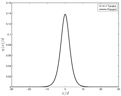
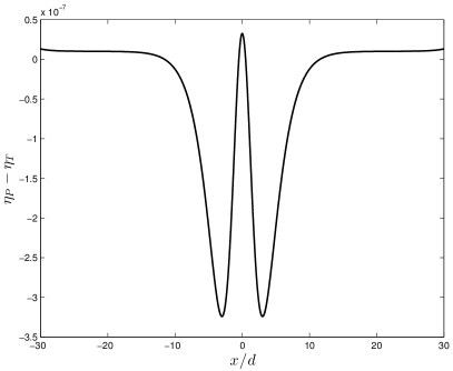
Figure 2. Comparison between Tanaka’s and the present solutions for the same Froude number $F_{T}=1.066365888477383$. Left: free surface; Right: difference (the vertical scale is $10^{-7}$).

Another feature of the conformal mapping consists in the easiness to obtain the velocity potential at the free surface along with the stream function needed, in particular, for transient computations [17, 30]:

$${\Phi}_{\text{s}}(x)\ \equiv\ \operatorname{Re}\/\{\/\Xi(x+\mathrm{i}\eta)\/\}\ =\ c\,X(\alpha,0),\qquad{\Psi}_{\text{s}}(x)\ \equiv\ \operatorname{Im}\/\{\/\Xi(x+\mathrm{i}\eta)\/\}\ =\ c\,Y(\alpha,0).$$

The graphs of the velocity potential and the stream function computed this way are plotted on Figure 3(a,b). We underline that these quantities can be obtained just by applying a few simple post-processing operations to the converged Babenko equation solution. By using similar explicit representation one can also compute the horizontal and vertical velocities computed at the free surface. They are represented for illustrative purposes on Figure 3 correspondingly (the solitary wave is the same for all plots on Figure 3).

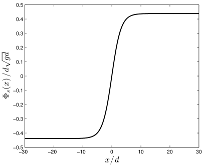
(a) Velocity potential

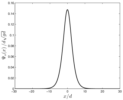
(b) Stream function

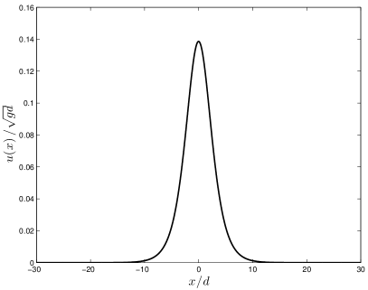
(c) Horizontal velocity

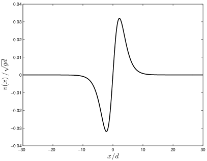
(d) Vertical velocity

Figure 3. The velocity potential, stream function, horizontal and vertical velocities evaluated at the free surface for the Froude number $F_{\mbox{\tiny\sc Tan}}=1.066365888477383$. (Note the different scales between the plots.)

Now, let us compare these numerical solutions with the available analytical results. Since we are dealing with a small amplitude solitary wave, we can apply the ninth-order Fenton asymptotic expansion [27] for the solitary wave speed $c^{2}$ in terms of its nonlinearity $\varepsilon=a/d$. So, we take the amplitude $a_{\mbox{\tiny\sc Pet}}/d=0.1382189387245723$ computed from the Babenko equation and, using Fenton’s expansion, we estimate the solitary wave speed for this amplitude:

$$c_{\mbox{\tiny\sc Fen}}\,/\,\sqrt{gd}\ =\ \textbf{1.066365888}5,\qquad c_{\mbox{\tiny\sc Pet}}\,/\,\sqrt{gd}\ =\ \textbf{1.066365888}477383,$$

where $c_{\mbox{\tiny\sc Pet}}$ is the solitary wave speed parameter used in the Petviashvili scheme. One can see that the differences between the predicted (Fenton) and prescribed (Petviashvili) values start to appear after the ninth digit, which is in perfect agreement with the order of the asymptotic expansion. However, strictly speaking, the Fenton solution is valid only in the limit $a/d\to 0$. On the other hand, the Babenko equation can be used to compute much more nonlinear solitary wave to the arbitrary precision. To illustrate the last statement we implemented the Petviashvili scheme using the Multiprecision Computing (MC) Toolbox for Matlab [29]. The transformations of the code needed to implement the arbitrary accuracy are really minimalistic. This constitutes one of the major advantages of the MC Toolbox.

In these higher-precision experiments, we take a periodic $\phi$-interval adapted for the increased accuracy ($30$ digits). Since the interval becomes longer, we have to increase also the number of Fourier modes up to $N=32\,768$. All floating point operations are done with $30$ significant digits (plus $3$ control digits). The tolerance parameter is set to $10^{-30}$. First, we compute the small solitary wave from previous examples using the extended arithmetics. We can compare the amplitudes with the standard double accuracy

$$a_{\mbox{\tiny\sc dp}}\,/\,d\ = \ \textbf{0.138218938724572}1,$$

$$a_{\mbox{\tiny\sc hp}}\,/\,d\ = \ \textbf{0.138218938724572}45734239592556073752.$$

One can see that the first 15 digits computed with the standard arithmetics are correct, which validates one more time the algorithm (we recall that the tolerance was set to $10^{-15}$ in the double precision computation).

However, it is much more challenging to compute high amplitude waves. The next example is inspired again by the Tanaka solution corresponding to the parameter $q_{c}=0.3$. The dimensionless speed of propagation of this soliton is approximatively equal to

$$c\,/\,\sqrt{gd}\ =\ 1.290941713543984.$$

By fixing this parameter in the Babenko equation, we start the Petviashvili iterations. The result is depicted on Figure 5(a) (solid line). The amplitude of this large solitary wave can be easily computed as well

$$a\,/\,d\ \approx\ 0.7583938551160400485984861886035\cdots.$$

However, this number is more difficult to validate, since in most studies the authors considered only solitary waves not higher than $a/d=0.7$ (see, for example, [42]). Nevertheless, we performed a comparison with the Tanaka solution. The results are shown on Figure 4. The maximal difference is of the order of $10^{-4}$ which is not completely satisfactory.

The computation of this large amplitude solitary wave took $2\,086$ iterations to converge to the tolerance $10^{-30}$ ($931$ iterations are needed to cross the standard $10^{-15}$ accuracy). The convergence rate of the iterative process is lower for high amplitude solitary waves. The $L_{\infty}$-norm of the difference between two successive iterations, along with the residual error are plotted on Figure 5(b). One can notice that the convergence to the small wave is much faster, even if the process is still converging. This point could be probably improved in future studies applying, for example, the generalized Petviashvili iteration [40]. Nevertheless, we have still a very good performance. For example, the computation of that large solitary wave to the standard $10^{-15}$ accuracy requires only $1.18\,$s (in terms of the CPU time) under Matlab. This timing is to be compared with Tanaka’s results.

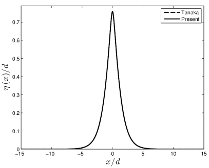
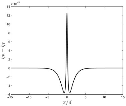
Figure 4. Comparison between Tanaka’s and the present solutions for the same Froude number $F_{T}=1.290941713543984$. Left: free surface; Right: difference (the vertical scale is $10^{-5}$).

For the sake of efficiency, we shall execute hereinafter the computations only within the standard double precision floating point arithmetics [38], unless the higher accuracy is explicitly required for some application.

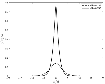
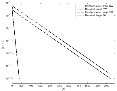
Figure 5. Two solitary waves computed in multiprecision arithmetics along with the convergence curves showing the decay of the error in $L_{\infty}$ norm.

3.3.1. Conserved integral quantities

Once the algorithm is validated, we can use it to produce some physically sound numerical results. The question we are addressing in this Section is the dependence of several important integral invariants (presented above in Section 2.2) on the wave amplitude. This question has already been addressed in previous studies essentially using asymptotic methods [43], which are formally valid only for the small amplitude waves. Our approach does not have such limitations and we are going to apply it to explore the whole range of wave heights.

First of all, on Figure 6 we present the so-called speed-amplitude relation — the abscissa represents the dimensionless amplitude of the wave, while the vertical axis shows the corresponding propagation speed. Our numerical result is compared to the classical Fenton ninth-order solution [27]. Again, from small to moderate solitary waves we obtain a very good agreement. For large amplitudes the advantage of our method becomes more explicit. Finally, on Figure 7(a)–(f) we show the dependence of the wave mass $\mathcal{M}$, circulation $\mathcal{C}$, kinetic energy $\mathcal{K}$, potential energy $\mathcal{V}_{g}$, impulse $\mathcal{I}$ and the total energy $\mathcal{E}$ correspondingly on the wave amplitude $a/d$. For instance, one can see that these quantities do not necessarily have the monotonic behaviour when the amplitude grows.

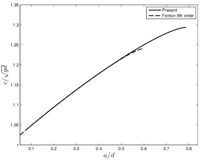
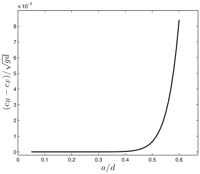
Figure 6. (a) Speed-amplitude relation for solitary gravity waves to the full Euler equations. Comparison with the Fenton ninth-order expansion. (b) Difference between Babenko and Fenton predictions for the speed-amplitude relations (the vertical scale on the right image (b) is $10^{-3}$).

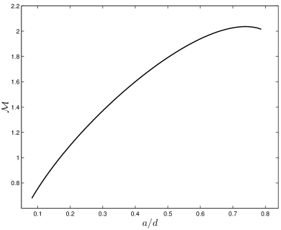
(a) Mass $\mathcal{M}$

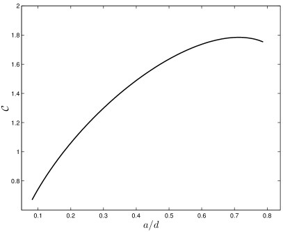
(b) Circulation $\mathcal{C}$

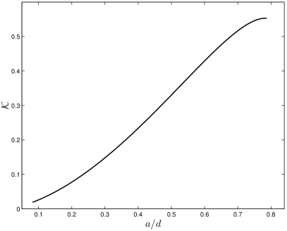
(c) Kinetic energy $\mathcal{K}$

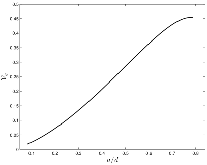
(d) Potential energy $\mathcal{V}_{g}$

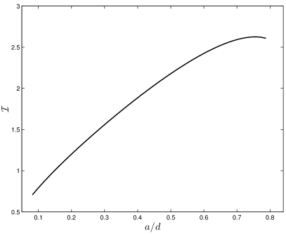
(e) Impulse $\mathcal{I}$

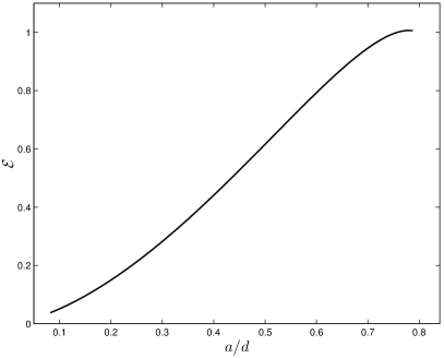
(f) Total energy $\mathcal{E}$

Figure 7. The dependence of several integral quantities for solitary waves on the wave amplitude.

Finally, the Babenko equation allows also to reconstruct efficiently various fields in the bulk of the fluid, as explained in Section 2.4. The computation of these fields amounts to perform post-processing operations on the fully converged solution. To illustrate this concept we take the large amplitude solitary wave represented on Figure 5(a). On Figure 8 we show the velocity potential (a) and the stream function (b) inside the fluid. The total (a) and dynamic (b) pressures are shown on Figure 9. The horizontal (a) and vertical (b) velocities along with accelerations are represented on Figures 10 and 11, correspondingly. Finally, the kinetic energy density (a) along with the total energy flux are shown on Figure 12. In particular, one can see from these computations that all presented fields (except the vertical velocity and horizontal acceleration) are symmetric with respect to the wave crest. On the other hand, two remaining quantities are antisymmetric with respect to the vertical axis passing through the crest. These results are in complete agreement with previous theoretical and numerical studies conducted with other methods [7, 11].

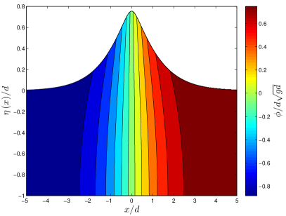
(a) Potential

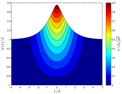
(b) Stream function

Figure 8. Equi-potentials (left) and iso-stream-function (right) under a large wave. Lines correspond to the iso-values computed in the ‘fixed’ Frame of reference where the the fluid is at rest in the far field $x\to\pm\infty$.

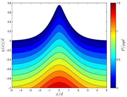
(a) Total pressure

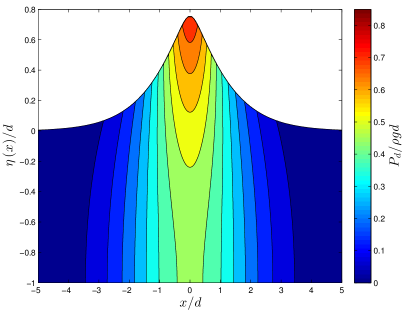
(b) Dynamic pressure

Figure 9. Isobars (left) and iso-dynamic-pressures $p+gy$ (right) under a large wave.

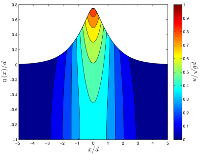
(a) Horizontal velocity

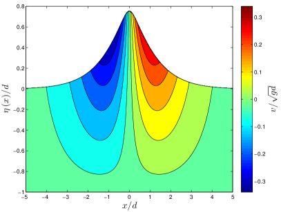
(b) Vertical velocity

Figure 10. Iso-horizontal (left) and iso-vertical (right) velocities under a large wave. Lines correspond to the iso-values computed in the ‘fixed’ Frame of reference where the the fluid is at rest in the far field $x\to\pm\infty$.

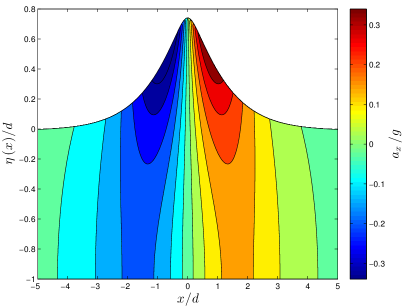
(a) Horizontal acceleration

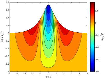
(b) Vertical acceleration

Figure 11. Iso-horizontal (left) and iso-vertical (right) accelerations under a large wave.

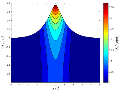
(a) Kinetic energy density

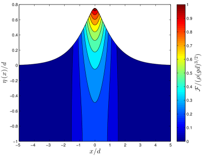
(b) Total energy flux

Figure 12. Iso-values of the kinetic energy density ${\textstyle{1\over 2}}(u^{2}+v^{2})$ (left) and the total energy flux $\bigl{(}p+gy+{\textstyle{1\over 2}}(u^{2}+v^{2})\bigr{)}u$ (right) under a large wave.

4.  Conclusions and perspectives

In the present paper, we proposed a fast and accurate method for computing steady gravity solitary waves to the full Euler equations. The method is based essentially on two main ingredients: first, a conformal mapping in order to reformulate the free surface Euler equations onto a fixed domain; second, the Petviashvili iterations to solve them numerically. The resulting scheme allows to compute the solution to any arbitrary accuracy using the multi-precision floating-point arithmetics [29]. Both ingredients are well known, but their combination turns out to be very efficient and seems to be new. We also compared our solution with some high-order asymptotic expansions [27, 43]. We obtain a good agreement for small and moderate amplitude solitary waves. For higher waves, the differences start to be noticeable. Moreover, the proposed method is compared to the classical Tanaka algorithm which is currently widely used in the water wave community [36, 14]. Our method outperforms the Tanaka algorithm in terms of the computational complexity (which results in much shorter CPU times) and the accuracy which is unlimited theoretically, but limited practically by the floating point arithmetics accuracy. The Matlab implementation is rather compact. The computational core is no longer than 50 lines of code. The script is freely available to download and to use for the scientific community through the Matlab Central File Exchange server [8].

Concerning the perspectives, the next step will consist in the inclusion of the capillary effects [19]. This new force introduces some inhomogeneous nonlinearities into the equations. The classical Petviashvili iterations, as it is presented hereinabove, fail to converge for capillary-gravity waves. In a upcoming study, we are going to propose a fix to this problem.

Acknowledgments

D. Dutykh acknowledges the support from ERC under the research project ERC-2011-AdG 290562-MULTIWAVE. The authors would like to thank also Angel Duran for very stimulating discussions on the Petviashvili method. Finally, we would like to thank Pavel Holodoborodko for invaluable help with the multi-precision floating point arithmetics.

References

- [1] K. I. Babenko. Some remarks on the theory of surface waves of finite amplitude. Sov. Math. Dokl., 35:599–603, 1987.
- [2] M. Chen. Exact Traveling-Wave Solutions to Bidirectional Wave Equations. International Journal of Theoretical Physics, 37:1547–1567, 1998.
- [3] M. Chen. Solitary-wave and multi pulsed traveling-wave solutions of Boussinesq systems. Applic. Analysis., 75:213–240, 2000.
- [4] W. Choi and R. Camassa. Exact Evolution Equations for Surface Waves. J. Eng. Mech., 125(7):756, 1999.
- [5] D. Clamond. Steady finite-amplitude waves on a horizontal seabed of arbitrary depth. J. Fluid Mech, 398:45–60, Nov. 1999.
- [6] D. Clamond. Cnoidal-type surface waves in deep water. J. Fluid Mech, 489:101–120, July 2003.
- [7] D. Clamond. Note on the velocity and related fields of steady irrotational two-dimensional surface gravity waves. Phil. Trans. R. Soc. A, 370(1964):1572–1586, Apr. 2012.
- [8] D. Clamond and D. Dutykh. http://www.mathworks.com/matlabcentral/fileexchange/39189-solitary-water-wave, 2012.
- [9] D. Clamond and D. Dutykh. Practical use of variational principles for modeling water waves. Physica D: Nonlinear Phenomena, 241(1):25–36, 2012.
- [10] D. Clamond and D. Dutykh. Fast accurate computation of the fully nonlinear solitary surface gravity waves. Submitted, pages 1–7, 2013.
- [11] A. Constantin, J. Escher, and H.-C. Hsu. Pressure Beneath a Solitary Water Wave: Mathematical Theory and Experiments. Archive for Rational Mechanics and Analysis, 201(1):251–269, Feb. 2011.
- [12] J. W. Cooley and J. W. Tukey. An algorithm for the machine calculation of complex Fourier series. Mathematics of Computation, 19(90):297–297, May 1965.
- [13] C. Cotter and O. Bokhove. Variational water-wave model with accurate dispersion and vertical vorticity. J. Eng. Math., 67(1-2):33–54, Oct. 2010.
- [14] W. Craig, P. Guyenne, J. Hammack, D. Henderson, and C. Sulem. Solitary water wave interactions. Phys. Fluids, 18(5):57106, 2006.
- [15] W. Craig and D. P. Nicholls. Traveling gravity water waves in two and three dimensions. European Journal of Mechanics - B/Fluids, 21(6):615–641, Nov. 2002.
- [16] W. Craig and P. Sternberg. Symmetry of solitary waves. Communications in Partial Differential Equations, 13(5):603–633, 1988.
- [17] W. Craig and C. Sulem. Numerical simulation of gravity waves. J. Comput. Phys., 108:73–83, 1993.
- [18] P. Cvitanović and B. Eckhardt. Periodic orbit expansions for classical smooth flows. J. Phys. A: Math. Gen., 24(5):L237–L241, Mar. 1991.
- [19] F. Dias and C. Kharif. Nonlinear gravity and capillary-gravity waves. Ann. Rev. Fluid Mech., 31:301–346, 1999.
- [20] F. Dias and P. Milewski. On the fully-nonlinear shallow-water generalized Serre equations. Physics Letters A, 374(8):1049–1053, 2010.
- [21] V. A. Dougalis, A. Durán, and D. E. Mitsotakis. Numerical approximation of solitary waves of the Benjamin equation. Mathematics and Computers in Simulation, Aug. 2012.
- [22] V. A. Dougalis and D. E. Mitsotakis. Theory and numerical analysis of Boussinesq systems: A review. In N. A. Kampanis, V. A. Dougalis, and J. A. Ekaterinaris, editors, Effective Computational Methods in Wave Propagation, pages 63–110. CRC Press, 2008.
- [23] P. G. Drazin and R. S. Johnson. Solitons: An introduction. Cambridge University Press, Cambridge, 1989.
- [24] D. Dutykh, D. Clamond, P. Milewski, and D. Mitsotakis. Finite volume and pseudo-spectral schemes for the fully nonlinear 1D Serre equations. Accepted to European Journal of Applied Mathematics, pages 1–27, 2013.
- [25] F. Fedele and D. Dutykh. Hamiltonian form and solitary waves of the spatial Dysthe equations. JETP Lett., 94(12):840–844, Oct. 2011.
- [26] F. Fedele and D. Dutykh. Special solutions to a compact equation for deep-water gravity waves. J. Fluid Mech, page 15, 2012.
- [27] J. Fenton. A ninth-order solution for the solitary wave. J. Fluid Mech, 53(2):257–271, 1972.
- [28] J. D. Fenton and M. M. Rienecker. A Fourier method for solving nonlinear water-wave problems: application to solitary-wave interactions. J. Fluid Mech., 118:411–443, Apr. 1982.
- [29] M. C. T. for MATLAB. v3.3.8.2611. Advanpix LLC., Tokyo, Japan, 2012.
- [30] D. Fructus, D. Clamond, O. Kristiansen, and J. Grue. An efficient model for threedimensional surface wave simulations. Part I: Free space problems. J. Comput. Phys., 205:665–685, 2005.
- [31] C. Gardner, J. Greene, M. Kruskal, and R. Miura. Method for Solving the Korteweg-deVries Equation. Phys. Rev. Lett, 19(19):1095–1097, Nov. 1967.
- [32] C. S. Gardner, J. M. Greene, M. D. Kruskal, and R. M. Miura. Korteweg-de Vries equation and Generalizations. VI. Methods for Exact Solution. Comm. Pure Appl. Math., 27:97–133, 1974.
- [33] M. Gedalin, T. Scott, and Y. Band. Optical Solitary Waves in the Higher Order Nonlinear Schrödinger Equation. Phys. Rev. Lett., 78(3):448–451, Jan. 1997.
- [34] J.-P. Germain. Contribution à l’étude de la houle en eau peu profonde. PhD thesis, Thèse de l’Université de Grenoble, France, 1967.
- [35] A. E. Green and P. M. Naghdi. A derivation of equations for wave propagation in water of variable depth. J. Fluid Mech., 78:237–246, 1976.
- [36] P. Helluy, F. Golay, J.-P. Caltagirone, P. Lubin, S. Vincent, D. Drevard, R. Marcer, P. Fraunie, N. Seguin, S. Grilli, A.-C. Lesage, A. Dervieux, and O. Allain. Numerical simulation of wave breaking. Mathematical Modelling and Numerical Analysis, 39(3):591–607, 2005.
- [37] E. Isaacson and H. B. Keller. Analysis of Numerical Methods. Dover Publications, 1966.
- [38] W. Kahan and J. Palmer. On a proposed floating-point standard. ACM SIGNUM Newsletter, 14(si-2):13–21, Oct. 1979.
- [39] E. A. Kuznetsov, A. M. Rubenchik, and V. E. Zakharov. Soliton stability in plasmas and hydrodynamics. Physics Reports, 142(3):103–165, Sept. 1986.
- [40] T. I. Lakoba and J. Yang. A generalized Petviashvili iteration method for scalar and vector Hamiltonian equations with arbitrary form of nonlinearity. J. Comp. Phys., 226:1668–1692, 2007.
- [41] M. A. Lavrent’ev and B. V. Shabat. Methoden der komplexen Funktionentheorie. Verlag Wissenschaft, 1967.
- [42] Y. A. Li, J. M. Hyman, and W. Choi. A Numerical Study of the Exact Evolution Equations for Surface Waves in Water of Finite Depth. Stud. Appl. Maths., 113:303–324, 2004.
- [43] M. Longuet-Higgins and J. Fenton. On the Mass, Momentum, Energy and Circulation of a Solitary Wave. II. Proc. R. Soc. A, 340(1623):471–493, 1974.
- [44] M. S. Longuet-Higgins. On the mass, momentum, energy and circulation of a solitary wave. Proc. R. Soc. Lond. A, 337:1–13, 1974.
- [45] M. S. Longuet-Higgins and M. Tanaka. On the crest instabilities of steep surface waves. J. Fluid Mech, 336:51–68, 1997.
- [46] K. E. Lonngren. Soliton experiments in plasmas. Plasma Physics, 25(9):943–982, Sept. 1983.
- [47] J. C. Luke. A variational principle for a fluid with a free surface. J. Fluid Mech., 27:375–397, 1967.
- [48] W. Malfliet. Solitary wave solutions of nonlinear wave equations. American Journal of Physics, 60(7):650, 1992.
- [49] J. McCowan. On the solitary wave. Phil. Mag. S., 32(194):45–58, 1891.
- [50] P. Milewski, J.-M. Vanden-Broeck, and Z. Wang. Dynamics of steep two-dimensional gravity-capillary solitary waves. J. Fluid Mech., 664:466–477, 2010.
- [51] R. M. Miura. The Korteweg-de Vries equation: a survey of results. SIAM Rev, 18:412–459, 1976.
- [52] H. Okamoto and M. Shoji. The Mathematical Theory of Permanent Progressive Water Waves. World Scientific, Singapore, 2001.
- [53] A. Osborne. Nonlinear ocean waves and the inverse scattering transform, volume 97. Elsevier, 2010.
- [54] G. W. Patrick. Relative equilibria in Hamiltonian systems: The dynamic interpretation of nonlinear stability on a reduced phase space. Journal of Geometry and Physics, 9(2):111–119, May 1992.
- [55] D. Pelinovsky and Y. A. Stepanyants. Convergence of Petviashvili’s iteration method for numerical approximation of stationary solutions of nonlinear wave equations. SIAM J. Num. Anal., 42:1110–1127, 2004.
- [56] V. I. Petviashvili. Equation of an extraordinary soliton. Sov. J. Plasma Phys., 2(3):469–472, 1976.
- [57] F. J. Seabra-Santos, A. M. Temperville, and D. P. Renouard. On the weak interaction of two solitary waves. Eur. J. Mech. B/Fluids, 8(2):103–115, 1989.
- [58] F. Serre. Contribution à l’étude des écoulements permanents et variables dans les canaux. La Houille blanche, 8:374–388, 1953.
- [59] V. P. Starr. Momentum and energy integrals for gravity waves of finite height. J. Mar. Res., 6:175–193, 1947.
- [60] M. Tanaka. The stability of solitary waves. Phys. Fluids, 29(3):650–655, 1986.
- [61] E. C. Titchmarsh. The Theory of Functions. Oxford University Press, 2nd editio edition, 1976.
- [62] L. N. Trefethen and D. Bau. Numerical linear algebra. SIAM, Philadelphia, 1997.
- [63] J.-M. Vanden-Broeck. Solitary waves in water: numerical methods and results. In Solitary waves in fluids, pages 55–84. 2007.
- [64] J. Yang. Nonlinear Waves in Integrable and Nonintegrable Systems. Society for Industrial and Applied Mathematics, Jan. 2010.
- [65] N. J. Zabusky and M. D. Kruskal. Interaction of solitons in a collisionless plasma and the recurrence of initial states. Phys. Rev. Lett, 15:240–243, 1965.
- [66] V. E. Zakharov and S. V. Manakov. On the complete integrability of a nonlinear Schrödinger equation. Teoret. Mat. Fiz., 19(3):332–343, 1974.