Effective interactions and fluctuation effects in spin-singlet superfluids

Abstract

We derive and evaluate one-loop functional flow equations for the effective interactions, self-energy and gap function in spin-singlet superfluids. The flow is generated by a fermionic frequency cutoff, which is supplemented by an external pairing field to treat divergencies associated with the Goldstone boson. To parametrize the singular momentum and frequency dependences of the effective interactions, the Nambu interaction vertex is decomposed in charge, magnetic, and normal and anomalous pairing channels. The one-loop flow solves reduced (mean-field) models for superfluidity exactly, and captures also important fluctuation effects. The Ward identity from charge conservation is generally violated, but can be enforced by projecting the flow. Applying the general formalism to the two-dimensional attractive Hubbard model, we obtain detailed results on the momentum and frequency dependences of the effective interactions for weak and moderate bare interactions. The gap is reduced by fluctuations, with a stronger reduction at weaker interactions, as expected.

PACS: 05.10.Cc, 71.10.Fd, 74.20.-z

I Introduction

Numerous interacting Fermi systems undergo a phase transition associated with spontaneous symmetry breaking at sufficiently low temperatures. Mean-field theory captures salient features of the symmetry-broken phase such as long-range order, quasi-particle excitations, and collective modes. For example, the BCS wave function provides a surprisingly faithful qualitative description of the superfluid ground state of an attractively interacting Fermi gas not only at weak, but also at strong coupling.eagles69 ; leggett80 Nevertheless, fluctuations often play an important role, both above and below the energy scale for symmetry breaking. At high energies, they renormalize the effective interactions generating an instability of the normal (symmetric) state, which may enhance or reduce the scale for symmetry breaking. At low energies, order parameter fluctuations usually suppress the order at least partially. Triggered by the possibility of designing tunable attractively interacting Fermi systems in cold atom traps, the issue of fluctuation effects in fermionic superfluids has attracted renewed interest.zwerger12

A framework to deal with fluctuation effects on all energy scales is provided by the functional renormalization group (fRG). This method provides a flexible source of new approximation schemes for interacting Fermi systems,metzner12 which are obtained by truncating the exact functional flow for the effective action as a function of a decreasing infrared cutoff $\Lambda$. wetterich93 ; berges02 ; kopietz10 The common types of spontaneous symmetry breaking such as superconductivity or magnetic order are associated with a divergence of the effective two-particle interaction at a finite scale $\Lambda_{c}$ in a specific momentum channel.zanchi00 ; halboth00 ; honerkamp01 To continue the flow below the scale $\Lambda_{c}$, an order parameter describing the broken symmetry has to be introduced.

A natural procedure is to decouple the interaction by a bosonic order parameter field, via a Hubbard-Stratonovich transformation, and to study the coupled flow of the fermionic and order parameter fields. Thereby order parameter fluctuations and also their interactions can be treated rather easily. This approach to symmetry breaking in the fRG framework has been explored already in several works on antiferromagnetic order baier04 ; krahl09a and superconductivity. birse05 ; diehl07 ; krippa07 ; strack08 ; floerchinger08 ; bartosch09 The bare microscopic interaction can usually be decoupled by introducing a single boson field. However, an effective interaction with only one bosonic field corresponds to a strongly simplified representation of the effective two-fermion interaction. Systems with competing instabilities corresponding to distinct order parameters require the introduction of several bosonic fields. krahl09b ; friederich10

Alternatively one may explore purely fermionic flows in the symmetry-broken phase. This can be done by adding an infinitesimal symmetry breaking term to the bare action, which is promoted to a finite order parameter below the scale $\Lambda_{c}$.salmhofer04 A simple one-loop truncation of the exact fRG flow equation with self-energy feedback was shown to yield an exact description of symmetry breaking for mean-field models such as the reduced BCS model, although the effective two-particle interactions diverge at the critical scale $\Lambda_{c}$.salmhofer04 ; gersch05 A subsequent application to the two-dimensional attractive Hubbard model showed that the same truncation, with a rather naive parametrization of the effective two-particle vertex, yields surprisingly accurate results for the superconducting gap at weak coupling.gersch08 However, the flow could be carried out down to $\Lambda=0$ only for a symmetry-breaking pairing field $\Delta_{0}$ above a certain minimal value. At that value a spurious divergence of the two-particle vertex was found. Fortunately, the minimal $\Delta_{0}$ was rather small, more than two orders of magnitude below the size of the gap at the end of the flow, and in this sense close to the ideal case of an infinitesimal $\Delta_{0}$.

In this paper we further develop the fermionic fRG for spin-singlet superfluids as a prototype for a broken continuous symmetry. We stay with the one-loop truncation used previously, but we derive and apply a much more accurate parametrization of the momentum and frequency dependence of the flowing two-particle vertex, taking all singularities in the particle-particle and particle-hole channel into account. We build on recent work on the structure of the Nambu two-particle vertex in a singlet superfluid,eberlein10 where constraints from symmetries (especially spin-rotation invariance) were derived, and insight into the singularities associated with superfluidity was gained by analyzing the exact fRG flow of a mean-field model with charge and spin forward scattering in addition to the reduced BCS interaction. Furthermore, a decomposition of the Nambu vertex in distinct interaction channels was derived, extending the decomposition formulated by Husemann and Salmhofer husemann09 for the normal state, karrasch08 which will now be used to separate regular from singular momentum and frequency dependences. With an adequate parametrization of the vertex at hand we can fully explore the performance of the one-loop truncated fermionic RG for symmetry-breaking beyond mean-field models. Explicit results for the effective interactions, the self-energy, and the gap function will be presented for the two-dimensional Hubbard model with an attractive interaction as a prototypical case. The Ward identity relating the gap to the vertex in the phase fluctuation channel (Goldstone mode) is not consistent with the truncated flow. The deviations are small at weak coupling, but they increase with the interaction strength. This problem can be treated by projecting the flow on the manifold of effective actions which respect the constraint imposed by the Ward identity. We also analyze to what extent effects of the Goldstone mode on other channels are captured by the one-loop truncation.

The article is structured as follows. In Sec. II the basic one-loop flow equations for the self-energy and the Nambu two-particle vertex are written down. Symmetry properties of the Nambu vertex following from spin rotation invariance and discrete symmetries are reviewed in Sec. III. The channel decomposition for spin-singlet superfluids is derived in Sec. IV, and the general structure of the flow equations is discussed. In Sec. V the random phase approximation is revisited in the framework of the channel decomposed flow equations. The general formalism is applied to the attractive Hubbard model in Sec. VI, with results for the self-energy, the gap function and the effective interactions in all channels. Merits and shortcomings of the channel decomposed one-loop flow equations are summarized in the conclusions, Sec. VII.

II Truncated flow equations

We analyze the superfluid ground state of attractively interacting spin-$\frac{1}{2}$ fermions. The system is specified by a bare action of the form

$${\cal S}[\psi,\bar{\psi}]=-\sum_{k,\sigma}[ik_{0}-\xi({\bf k})]\,\bar{\psi}_{k\sigma}\psi_{k\sigma}+{\cal U}[\psi,\bar{\psi}]\;,$$ (1)

where $\bar{\psi}_{k\sigma}$ and $\psi_{k\sigma}$ are Grassmann variables associated with creation and annihilation operators, respectively. The variable $k=(k_{0},{\bf k})$ contains the Matsubara frequency $k_{0}$ in addition to the momentum ${\bf k}$, and $\sigma$ denotes the spin orientation. $\xi({\bf k})=\epsilon({\bf k})-\mu$ is the single-particle energy relative to the chemical potential, and ${\cal U}[\psi,\bar{\psi}]$ describes a spin-rotation invariant two-particle interaction

$${\cal U}[\psi,\bar{\psi}] = \frac{1}{4}\sum_{k_{i},\sigma_{i}}\big{[}U(k_{1},k_{2},k_{3},k_{4})\delta_{\sigma_{1}\sigma_{4}}\delta_{\sigma_{2}\sigma_{3}}-U(k_{1},k_{2},k_{4},k_{3})\delta_{\sigma_{1}\sigma_{3}}\delta_{\sigma_{2}\sigma_{4}}\big{]}$$ (2)

$$\times \bar{\psi}_{k_{1}\sigma_{1}}\bar{\psi}_{k_{2}\sigma_{2}}\psi_{k_{3}\sigma_{3}}\psi_{k_{4}\sigma_{4}}\;.$$

Here and below, all temperature and volume factors are incorporated in the summation symbols.

Our analysis is based on a truncation of the exact flow equation wetterich93 ; metzner12 for the effective action $\Gamma^{\Lambda}[\psi,\bar{\psi}]$, that is, the generating functional for one-particle irreducible vertex functions in the presence of an infrared cutoff $\Lambda$. The cutoff is implemented by adding a regulator function to the inverse of the bare propagator. The effective action $\Gamma^{\Lambda}[\psi,\bar{\psi}]$ interpolates between the regularized bare action at the initial scale $\Lambda_{0}$ and the final effective action $\Gamma[\psi,\bar{\psi}]$ in the limit $\Lambda\to 0$. Spontaneous breaking of the $U(1)$ charge symmetry in the superfluid state can be treated by adding a small (ultimately infinitesimal) symmetry breaking field

$$\delta{\cal S}[\psi,\bar{\psi}]=\sum_{k}\left[\Delta_{0}(k)\bar{\psi}_{-k\downarrow}\bar{\psi}_{k\uparrow}+\Delta_{0}^{*}(k)\psi_{k\uparrow}\psi_{-k\downarrow}\right]$$ (3)

to the bare action, which is then promoted to a finite order parameter in the course of the flow.salmhofer04

Expanding the exact functional flow equation for $\Gamma^{\Lambda}[\psi,\bar{\psi}]$ in powers of the source fields $\psi$ and $\bar{\psi}$, one obtains a hierarchy of flow equations for the n-particle vertex functions. metzner12 We truncate the hierarchy at the two-particle level, including however self-energy corrections generated from contractions of three-particle terms.katanin04 This truncation was used in all previous fermionic fRG studies of symmetry breaking.salmhofer04 ; gersch05 ; gersch08 ; eberlein10 It is exact for mean-field models. Our description of the truncation follows closely the presentation in Ref. eberlein10, . However, we use notations as in Ref. metzner12, , where the regulator function is fully included in the two-point vertex ${\bf\Gamma}^{(2)\Lambda}$, and the sign convention for ${\bf\Gamma}^{(2)\Lambda}$ and the propagator ${\bf G}^{\Lambda}$ differs from that used in Ref. eberlein10, .

In a superfluid state it is convenient to use Nambu spinors $\phi_{ks}$ and $\bar{\phi}_{ks}$ defined as

$$\bar{\phi}_{k+}=\bar{\psi}_{k\uparrow},\quad\phi_{k+}=\psi_{k\uparrow},\quad\bar{\phi}_{k-}=\psi_{-k\downarrow},\quad\phi_{k-}=\bar{\psi}_{-k\downarrow}$$ (4)

instead of $\psi_{k\sigma}$ and $\bar{\psi}_{k\sigma}$ as a basis. The effective action as a functional of the Nambu fields, truncated beyond quartic (two-particle) terms, has the form

$$\Gamma^{\Lambda}[\phi,\bar{\phi}] = \Gamma^{(0)\Lambda}-\sum_{k}\sum_{s_{1},s_{2}}\Gamma_{s_{1}s_{2}}^{(2)\Lambda}(k)\,\bar{\phi}_{ks_{1}}\phi_{ks_{2}}$$ (5)

$$+ \frac{1}{4}\sum_{k_{1},\dots,k_{4}}\sum_{s_{1},\dots,s_{4}}\Gamma_{s_{1}s_{2}s_{3}s_{4}}^{(4)\Lambda}(k_{1},k_{2},k_{3},k_{4})\,\bar{\phi}_{k_{1}s_{1}}\bar{\phi}_{k_{2}s_{2}}\phi_{k_{3}s_{3}}\phi_{k_{4}s_{4}}\;,$$

where $\Gamma^{(0)\Lambda}$ yields the grand canonical potential. For spin-singlet pairing with unbroken spin-rotation invariance only terms with an equal number of $\phi$ and $\bar{\phi}$ fields contribute. The Nambu vertex $\Gamma_{s_{1}s_{2}s_{3}s_{4}}^{(4)\Lambda}(k_{1},k_{2},k_{3},k_{4})$ is non-zero only for $k_{1}+k_{2}=k_{3}+k_{4}$, due to translation invariance. The (scale-dependent) Nambu propagator ${\bf G}^{\Lambda}$ is related to ${\bf\Gamma}^{(2)\Lambda}$ by $({\bf G}^{\Lambda})^{-1}={\bf\Gamma}^{(2)\Lambda}$, and can be written as a $2\times 2$ matrix

$${\bf G}^{\Lambda}(k)=\left(\begin{array}[]{cc}G_{++}^{\Lambda}(k)&G_{+-}^{\Lambda}(k)\\ G_{-+}^{\Lambda}(k)&G_{--}^{\Lambda}(k)\end{array}\right)=\left(\begin{array}[]{cc}G^{\Lambda}(k)&F^{\Lambda}(k)\\ F^{*\Lambda}(k)&-G^{\Lambda}(-k)\end{array}\right)\;.$$ (6)

The anomalous propagator $F^{\Lambda}(k)$ is a symmetric function of $k_{0}$ and ${\bf k}$. The Nambu self-energy ${\bf\Sigma}^{\Lambda}$ is defined by the Dyson equation $({\bf G}^{\Lambda})^{-1}=({\bf G}_{0}^{\Lambda})^{-1}-{\bf\Sigma}^{\Lambda}$, where ${\bf G}_{0}^{\Lambda}$ is the bare regularized propagator (in presence of $\Delta_{0}$). In the superfluid state it has the form

$${\bf\Sigma}^{\Lambda}(k)=\left(\begin{array}[]{cc}\Sigma^{\Lambda}(k)&\Delta_{0}(k)-\Delta^{\Lambda}(k)\\ \Delta_{0}^{*}(k)-\Delta^{*\Lambda}(k)&-\Sigma^{\Lambda}(-k)\end{array}\right)\;,$$ (7)

where $\Sigma^{\Lambda}(k)$ is the normal component of the self-energy and $\Delta^{\Lambda}(k)$ is the (flowing) gap function.

The gap function and the Nambu vertex are related by a Ward identity following from global charge conservation (see, for example, Ref. salmhofer04, )

$$\Delta^{\Lambda}(k)-\Delta_{0}(k) = \sum_{k^{\prime}}\sum_{s,s^{\prime}}\left[\Delta_{0}(k^{\prime})G^{\Lambda}_{s+}(k^{\prime})G^{\Lambda}_{-s^{\prime}}(k^{\prime})-\Delta_{0}^{*}(k^{\prime})G^{\Lambda}_{s-}(k^{\prime})G^{\Lambda}_{+s^{\prime}}(k^{\prime})\right]$$ (8)

$$\times\,\Gamma^{(4)\Lambda}_{+s^{\prime}s-}(k,k^{\prime},k^{\prime},k)\;.$$

The Ward identity implies that some components of the Nambu vertex diverge in case of spontaneous symmetry breaking ($\Delta^{\Lambda}$ finite for $\Delta_{0}\to 0$), which is a manifestation of the massless Goldstone boson.

The flow equation for the Nambu self-energy is given by

$$\frac{d}{d\Lambda}\Sigma_{s_{1}s_{2}}^{\Lambda}(k)=\sum_{k^{\prime}}\sum_{s^{\prime}_{1},s^{\prime}_{2}}S_{s^{\prime}_{2}s^{\prime}_{1}}^{\Lambda}(k^{\prime})\Gamma^{(4)\Lambda}_{s_{1}s^{\prime}_{1}s^{\prime}_{2}s_{2}}(k,k^{\prime},k^{\prime},k)\;,$$ (9)

where

$${\bf S}^{\Lambda}(k) = \left.\frac{d}{d\Lambda}{\bf G}^{\Lambda}(k)\right|_{{\bf\Sigma}^{\Lambda}\,{\rm fixed}}$$ (10)

$$= \left[1-{\bf G}_{0}^{\Lambda}(k){\bf\Sigma}^{\Lambda}(k)\right]^{-1}\frac{d{\bf G}_{0}^{\Lambda}(k)}{d\Lambda}\left[1-{\bf\Sigma}^{\Lambda}(k){\bf G}_{0}^{\Lambda}(k)\right]^{-1}$$

is the so-called single-scale propagator. The truncated flow equation for the Nambu vertex (see Fig. 1) reads

$$\frac{d}{d\Lambda}\Gamma^{(4)\Lambda}_{s_{1}s_{2}s_{3}s_{4}}(k_{1},k_{2},k_{3},k_{4}) = \Pi^{\rm PH,d}_{s_{1}s_{2}s_{3}s_{4}}(k_{1},k_{2},k_{3},k_{4})-\Pi^{\rm PH,cr}_{s_{1}s_{2}s_{3}s_{4}}(k_{1},k_{2},k_{3},k_{4})$$ (11)

$$- \frac{1}{2}\Pi^{\rm PP}_{s_{1}s_{2}s_{3}s_{4}}(k_{1},k_{2},k_{3},k_{4})\;,$$

where

$$\Pi^{\rm PH,d}_{s_{1}s_{2}s_{3}s_{4}}(k_{1},k_{2},k_{3},k_{4}) = \sum_{p,q}\sum_{s^{\prime}_{1},\dots,s^{\prime}_{4}}\frac{d}{d\Lambda}[G^{\Lambda}_{s^{\prime}_{1}s^{\prime}_{2}}(p)G^{\Lambda}_{s^{\prime}_{3}s^{\prime}_{4}}(q)]$$ (12)

$$\times \Gamma^{(4)\Lambda}_{s_{1}s^{\prime}_{2}s^{\prime}_{3}s_{4}}(k_{1},p,q,k_{4})\Gamma^{(4)\Lambda}_{s^{\prime}_{4}s_{2}s_{3}s^{\prime}_{1}}(q,k_{2},k_{3},p)\;,$$

$$\Pi^{\rm PH,cr}_{s_{1}s_{2}s_{3}s_{4}}(k_{1},k_{2},k_{3},k_{4}) = \sum_{p,q}\sum_{s^{\prime}_{1},\dots,s^{\prime}_{4}}\frac{d}{d\Lambda}[G^{\Lambda}_{s^{\prime}_{1}s^{\prime}_{2}}(p)G^{\Lambda}_{s^{\prime}_{3}s^{\prime}_{4}}(q)]$$ (13)

$$\times \Gamma^{(4)\Lambda}_{s_{2}s^{\prime}_{2}s^{\prime}_{3}s_{4}}(k_{2},p,q,k_{4})\Gamma^{(4)\Lambda}_{s^{\prime}_{4}s_{1}s_{3}s^{\prime}_{1}}(q,k_{1},k_{3},p)\;,$$

$$\Pi^{\rm PP}_{s_{1}s_{2}s_{3}s_{4}}(k_{1},k_{2},k_{3},k_{4}) = \sum_{p,q}\sum_{s^{\prime}_{1},\dots,s^{\prime}_{4}}\frac{d}{d\Lambda}[G^{\Lambda}_{s^{\prime}_{1}s^{\prime}_{2}}(p)G^{\Lambda}_{s^{\prime}_{3}s^{\prime}_{4}}(q)]$$ (14)

$$\times \Gamma^{(4)\Lambda}_{s_{1}s_{2}s^{\prime}_{3}s^{\prime}_{1}}(k_{1},k_{2},q,p)\Gamma^{(4)\Lambda}_{s^{\prime}_{2}s^{\prime}_{4}s_{3}s_{4}}(p,q,k_{3},k_{4})\;.$$

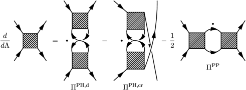
Figure 1: Feynman diagrams representing the flow equation for the two-particle vertex. The dots denote differentiation of the propagator products with respect to the scale $\Lambda$.

The flow equation for the self-energy is exact (for an exact $\Gamma^{(4)\Lambda}$), while in the flow of $\Gamma^{(4)\Lambda}$ contributions from $\Gamma^{(6)\Lambda}$ beyond self-energy feedback have been discarded.katanin04 ; metzner12 These discarded contributions are at least of order $(\Gamma^{(4)\Lambda})^{3}$, and they involve overlapping loops leading to a reduced momentum integration volume. The truncation is exact for mean-field models with a reduced BCS and/or forward scattering interaction, although $\Gamma^{(4)\Lambda}$ becomes large at the critical scale. salmhofer04 ; gersch08 ; eberlein10 Particle-particle terms in Nambu representation contain particle-hole contributions in the original fermion basis and vice versa. In particular, the particle-particle contribution generating the Cooper instability is captured by the Nambu particle-hole diagrams.

III Symmetries of Nambu vertex

The Nambu vertex $\Gamma_{s_{1}s_{2}s_{3}s_{4}}^{(4)\Lambda}(k_{1},k_{2},k_{3},k_{4})$ has 16 components corresponding to the choices $s_{i}=\pm$ for $i=1,\dots,4$. Spin rotation invariance reduces the number of independent components of the Nambu vertex substantially. In Ref. eberlein10, it was shown that the vertex can be parametrized by three functions of $k_{1},k_{2},k_{3},k_{4}$, where $k_{1}+k_{2}=k_{3}+k_{4}$ for translation invariant systems. These functions are further constrained by discrete symmetries. In this section we describe the spin-rotation invariant form of the Nambu vertex as derived in Ref. eberlein10, .

In addition to the normal interaction, in the $U(1)$ symmetry-broken state there are also anomalous interactions corresponding to operator products $\bar{\psi}\bar{\psi}\bar{\psi}\bar{\psi}$ + conjugate and $\bar{\psi}\bar{\psi}\bar{\psi}\psi$ + conjugate.salmhofer04 ; gersch08 Following Ref. eberlein10, , we write down spin-rotation invariant forms for the normal and anomalous interaction terms in the $\psi$-basis, and then the corresponding expressions in Nambu representation.

A spin-rotation invariant normal interaction can always be expressed as salmhofer01

$$\Gamma^{(2+2)}[\psi,\bar{\psi}] = \frac{1}{4}\sum_{k_{i},\sigma_{i}}\left[V(k_{1},k_{2},k_{3},k_{4})\delta_{\sigma_{1}\sigma_{4}}\delta_{\sigma_{2}\sigma_{3}}-V(k_{1},k_{2},k_{4},k_{3})\delta_{\sigma_{1}\sigma_{3}}\delta_{\sigma_{2}\sigma_{4}}\right]$$ (15)

$$\times \bar{\psi}_{k_{1}\sigma_{1}}\bar{\psi}_{k_{2}\sigma_{2}}\psi_{k_{3}\sigma_{3}}\psi_{k_{4}\sigma_{4}}\;.$$

Here and in the remainder of this section we suppress the superscript $\Lambda$ for the scale dependence. One may also write $\Gamma^{(2+2)}[\psi,\bar{\psi}]$ as a sum of a spin singlet and a spin triplet component halboth00

$$\Gamma^{(2+2)}[\psi,\bar{\psi}] = \frac{1}{4}\sum_{k_{i},\sigma_{i}}\left[V^{S}(k_{1},k_{2},k_{3},k_{4})\,S_{\sigma_{1}\sigma_{2}\sigma_{3}\sigma_{4}}+V^{T}(k_{1},k_{2},k_{3},k_{4})\,T_{\sigma_{1}\sigma_{2}\sigma_{3}\sigma_{4}}\right]$$ (16)

$$\times \bar{\psi}_{k_{1}\sigma_{1}}\bar{\psi}_{k_{2}\sigma_{2}}\psi_{k_{3}\sigma_{3}}\psi_{k_{4}\sigma_{4}}\;,$$

where $S_{\sigma_{1}\sigma_{2}\sigma_{3}\sigma_{4}}=\frac{1}{2}(\delta_{\sigma_{1}\sigma_{4}}\delta_{\sigma_{2}\sigma_{3}}-\delta_{\sigma_{1}\sigma_{3}}\delta_{\sigma_{2}\sigma_{4}})$, $T_{\sigma_{1}\sigma_{2}\sigma_{3}\sigma_{4}}=\frac{1}{2}(\delta_{\sigma_{1}\sigma_{4}}\delta_{\sigma_{2}\sigma_{3}}+\delta_{\sigma_{1}\sigma_{3}}\delta_{\sigma_{2}\sigma_{4}})$, and

$$V^{S}(k_{1},k_{2},k_{3},k_{4}) = V(k_{1},k_{2},k_{3},k_{4})+V(k_{1},k_{2},k_{4},k_{3})\;,$$ (17)

$$V^{T}(k_{1},k_{2},k_{3},k_{4}) = V(k_{1},k_{2},k_{3},k_{4})-V(k_{1},k_{2},k_{4},k_{3})\;.$$ (18)

A spin-rotation invariant anomalous interaction with four creation (or annihilation) operators can be written in the form eberlein10

$$\Gamma^{(4+0)}[\psi,\bar{\psi}]=$$

$$\frac{1}{8}\sum_{k_{i}} \Big{\{}W^{S}(k_{1},k_{2},k_{3},k_{4})(\bar{\psi}_{k_{1}\uparrow}\bar{\psi}_{k_{2}\downarrow}-\bar{\psi}_{k_{1}\downarrow}\bar{\psi}_{k_{2}\uparrow})(\bar{\psi}_{k_{3}\uparrow}\bar{\psi}_{k_{4}\downarrow}-\bar{\psi}_{k_{3}\downarrow}\bar{\psi}_{k_{4}\uparrow})$$

$$- \,W^{T}(k_{1},k_{2},k_{3},k_{4})\big{[}(\bar{\psi}_{k_{1}\uparrow}\bar{\psi}_{k_{2}\downarrow}+\bar{\psi}_{k_{1}\downarrow}\bar{\psi}_{k_{2}\uparrow})(\bar{\psi}_{k_{3}\uparrow}\bar{\psi}_{k_{4}\downarrow}+\bar{\psi}_{k_{3}\downarrow}\bar{\psi}_{k_{4}\uparrow})$$ (19)

$$-2(\bar{\psi}_{k_{1}\uparrow}\bar{\psi}_{k_{2}\uparrow}\bar{\psi}_{k_{3}\downarrow}\bar{\psi}_{k_{4}\downarrow}+\bar{\psi}_{k_{1}\downarrow}\bar{\psi}_{k_{2}\downarrow}\bar{\psi}_{k_{3}\uparrow}\bar{\psi}_{k_{4}\uparrow})\big{]}+{\rm conj.}\Big{\}}\;.$$

Conjugated terms denoted by ”conj.” are obtained by reversing the order of fields, replacing $\bar{\psi}_{k\sigma}$ by $\psi_{k^{*}\sigma}$, and complex conjugation of the functions $W^{S,T}$.

Finally, spin-rotation invariant anomalous interactions with three creation and one annihilation operators, or vice versa, can be written as eberlein10

$$\Gamma^{(3+1)}[\psi,\bar{\psi}] = \frac{1}{2}\sum_{k_{i}}\Big{\{}X^{S}(k_{1},k_{2},k_{3},k_{4})\sum_{\sigma}\bar{\psi}_{k_{1}\sigma}(\bar{\psi}_{k_{2}\uparrow}\bar{\psi}_{k_{3}\downarrow}-\bar{\psi}_{k_{2}\downarrow}\bar{\psi}_{k_{3}\uparrow})\psi_{k_{4}\sigma}$$ (20)

$$+\;X^{T}(k_{1},k_{2},k_{3},k_{4})\Big{[}\sum_{\sigma}\epsilon_{\sigma}\bar{\psi}_{k_{1}\sigma}(\bar{\psi}_{k_{2}\uparrow}\bar{\psi}_{k_{3}\downarrow}+\bar{\psi}_{k_{2}\downarrow}\bar{\psi}_{k_{3}\uparrow})\psi_{k_{4}\sigma}$$

$$\quad+\;2(\bar{\psi}_{k_{1}\uparrow}\bar{\psi}_{k_{2}\downarrow}\bar{\psi}_{k_{3}\downarrow}\psi_{k_{4}\downarrow}-\bar{\psi}_{k_{1}\downarrow}\bar{\psi}_{k_{2}\uparrow}\bar{\psi}_{k_{3}\uparrow}\psi_{k_{4}\uparrow})\Big{]}+{\rm conj.}\Big{\}}\;,$$

where $\epsilon_{\uparrow}=1$ and $\epsilon_{\downarrow}=-1$.

It is convenient to collect the 16 components of the Nambu vertex $\Gamma_{s_{1}s_{2}s_{3}s_{4}}^{(4)}$ in a $4\times 4$ matrix

$${\bf\Gamma}^{(4)}=\left(\begin{array}[]{cccc}\Gamma_{++++}^{(4)}&\Gamma_{++-+}^{(4)}&\Gamma_{+-++}^{(4)}&\Gamma_{+--+}^{(4)}\\[5.69054pt] \Gamma_{+++-}^{(4)}&\Gamma_{++--}^{(4)}&\Gamma_{+-+-}^{(4)}&\Gamma_{+---}^{(4)}\\[5.69054pt] \Gamma_{-+++}^{(4)}&\Gamma_{-+-+}^{(4)}&\Gamma_{--++}^{(4)}&\Gamma_{---+}^{(4)}\\[5.69054pt] \Gamma_{-++-}^{(4)}&\Gamma_{-+--}^{(4)}&\Gamma_{--+-}^{(4)}&\Gamma_{----}^{(4)}\end{array}\right)\quad.$$ (21)

Rows in this matrix are labeled by $s_{1}$ and $s_{4}$, while columns are labeled by $s_{2}$ and $s_{3}$. With this convention the Bethe-Salpeter equation yielding the exact Nambu vertex in reduced (mean-field) models can be written as a matrix equation.eberlein10 Translating the spin-rotation invariant structure of the various interaction terms to the Nambu representation, one obtains the Nambu vertex in the following form fn2

$${\bf\Gamma}^{(4)}(k_{1},k_{2},k_{3},k_{4})=\hskip 347.12354pt$$

$$\left(\begin{array}[]{cccc}V^{T}(k_{1},k_{2},k_{3},k_{4})&X(k_{1},k_{2},k_{3},k_{4})&X^{*}(k^{*}_{4},k^{*}_{3},k^{*}_{2},k^{*}_{1})&\!\!-V(k_{1},-k_{3},-k_{2},k_{4})\\[5.69054pt] \!\!-X(k_{1},k_{2},k_{4},k_{3})&W(k_{1},k_{2},k_{3},k_{4})&V(k_{1},-k_{4},-k_{2},k_{3})&X^{*}(k_{4},k_{3},k_{1},k_{2})\\[5.69054pt] \!\!-X^{*}(k^{*}_{4},k^{*}_{3},k^{*}_{2},k^{*}_{1})&V^{*}(k_{1},-k_{4},-k_{2},k_{3})&W^{*}(k^{*}_{4},k^{*}_{3},k^{*}_{2},k^{*}_{1})&X(k^{*}_{1},k^{*}_{2},k^{*}_{3},k^{*}_{4})\\[5.69054pt] \!\!-V^{*}(k_{1},-k_{3},-k_{2},k_{4})&\!\!-X^{*}(k_{4},k_{3},k_{2},k_{1})&\!\!-X(k^{*}_{1},k^{*}_{2},k^{*}_{3},k^{*}_{4})&V^{T*}(k_{1},k_{2},k_{3},k_{4})\end{array}\right)\;,$$ (26)

where $k^{*}=(-k_{0},{\bf k})$. The matrix elements $W$ and $X$ are related to the anomalous (4+0) and (3+1) interactions, respectively:

$$W(k_{1},k_{2},k_{3},k_{4}) = W^{S}(k_{1},-k_{4},-k_{3},k_{2})-W^{S}(k_{1},-k_{3},-k_{4},k_{2})$$ (28)

$$+ W^{T}(k_{1},-k_{4},-k_{3},k_{2})-W^{T}(k_{1},-k_{3},-k_{4},k_{2})$$

$$+ 2W^{T}(k_{1},k_{2},-k_{3},-k_{4})\;,$$

$$X(k_{1},k_{2},k_{3},k_{4}) = X^{S}(k_{1},k_{2},-k_{3},k_{4})-X^{S}(k_{2},k_{1},-k_{3},k_{4})$$ (29)

$$+ X^{T}(k_{1},k_{2},-k_{3},k_{4})-X^{T}(k_{2},k_{1},-k_{3},k_{4})$$

$$+ 2X^{T}(-k_{3},k_{2},k_{1},k_{4})\;.$$

For translation invariant systems the functions $V(k_{1},k_{2},k_{3},k_{4})$, $W(k_{1},k_{2},k_{3},k_{4})$ and $X(k_{1},k_{2},k_{3},k_{4})$ are non-zero only if $k_{1}+k_{2}=k_{3}+k_{4}$, and can therefore be parametrized by three energy and momentum variables. Discrete symmetries, such as time reversal and reflection invariance, and the antisymmetry under particle exchange further constrain the functions parametrizing the Nambu vertex.eberlein10

IV Channel decomposition

The two-particle vertex acquires a pronounced momentum and frequency dependence in the course of the flow, which becomes even singular at the critical scale for spontaneous symmetry breaking. A parametrization based on weak coupling power counting is not adequate in this situation. Keeping the full dependence on the three independent momenta and frequencies is technically not feasible. The particle-particle and particle-hole contributions to the flow, Eq. (11), depend strongly on certain linear combinations of momenta and frequencies, namely

$$\Pi^{\rm PH,d}_{s_{1}s_{2}s_{3}s_{4}}(k_{1},k_{2},k_{3},k_{4}) : \;k_{3}-k_{2}\;,$$

$$\Pi^{\rm PH,cr}_{s_{1}s_{2}s_{3}s_{4}}(k_{1},k_{2},k_{3},k_{4}) : \;k_{3}-k_{1}\;,$$

$$\Pi^{\rm PP}_{s_{1}s_{2}s_{3}s_{4}}(k_{1},k_{2},k_{3},k_{4}) : \;k_{1}+k_{2}\;.$$ (30)

This is because the poles of the contributing propagators coalesce when the above combinations of momenta and frequencies vanish or are situated at special nesting points (in case of nested Fermi surfaces). We therefore write the vertex as a sum of interaction channels, where each channel carries one potentially singular momentum dependence, which can be parametrized accurately, while the dependence on the remaining two momentum variables is treated more crudely. This channel decomposition was introduced by Husemann and Salmhofer husemann09 for the two-particle vertex in a normal metallic state,karrasch08 and extended by us for a superfluid state. eberlein10 Most recently it was also formulated for an antiferromagnetic state.maier12

IV.1 Interaction channels

Following Husemann and Salmhofer,husemann09 we write the normal vertex in the form

$$\Gamma^{(2+2)\Lambda}[\psi,\bar{\psi}] = {\cal U}[\psi,\bar{\psi}]$$ (31)

$$+ \frac{1}{2}\,{\sum_{k_{i}}}^{\prime}\,C^{\Lambda}_{\frac{k_{1}+k_{4}}{2},\frac{k_{2}+k_{3}}{2}}(k_{3}-k_{2})\sum_{\sigma,\sigma^{\prime}}\bar{\psi}_{k_{1}\sigma}\bar{\psi}_{k_{2}\sigma^{\prime}}\psi_{k_{3}\sigma^{\prime}}\psi_{k_{4}\sigma}$$

$$+ \frac{1}{2}\,{\sum_{k_{i}}}^{\prime}\,M^{\Lambda}_{\frac{k_{1}+k_{4}}{2},\frac{k_{2}+k_{3}}{2}}(k_{3}-k_{2})\sum_{\sigma_{i}}\vec{\tau}_{\sigma_{1}\sigma_{4}}\cdot\vec{\tau}_{\sigma_{2}\sigma_{3}}\,\bar{\psi}_{k_{1}\sigma_{1}}\bar{\psi}_{k_{2}\sigma_{2}}\psi_{k_{3}\sigma_{3}}\psi_{k_{4}\sigma_{4}}$$

$$+ \frac{1}{2}\,{\sum_{k_{i}}}^{\prime}\,P^{\Lambda}_{\frac{k_{1}-k_{2}}{2},\frac{k_{4}-k_{3}}{2}}(k_{1}+k_{2})\sum_{\sigma,\sigma^{\prime}}\bar{\psi}_{k_{1}\sigma}\bar{\psi}_{k_{2}\sigma^{\prime}}\psi_{k_{3}\sigma^{\prime}}\psi_{k_{4}\sigma}\;,\hskip 14.22636pt$$

where ${\cal U}[\psi,\bar{\psi}]$ is the bare interaction, and the coupling functions $C^{\Lambda}$, $M^{\Lambda}$, and $P^{\Lambda}$ capture the “charge”, “magnetic” (spin), and “pairing” channels, respectively. The matrices collected in $\vec{\tau}=(\tau^{x},\tau^{y},\tau^{z})$ are the three Pauli matrices. The prime at the sums over $k_{i}$ indicates momentum (and frequency) conservation, $k_{1}+k_{2}=k_{3}+k_{4}$. The momentum argument in brackets is the momentum transfer for the charge and magnetic channels, and the total momentum for the pairing channel. These are the variables for which a singular dependence is expected. Comparing the ansatz Eq. (31) to the general spin-rotation invariant form of the normal vertex Eq. (15), written in terms of $V^{\Lambda}(k_{1},k_{2},k_{3},k_{4})$, one obtains the relation

$$V^{\Lambda}(k_{1},k_{2},k_{3},k_{4}) = U(k_{1},k_{2},k_{3},k_{4})$$ (32)

$$+ \Big{[}C^{\Lambda}_{\frac{k_{1}+k_{4}}{2},\frac{k_{2}+k_{3}}{2}}(k_{3}-k_{2})+P^{\Lambda}_{\frac{k_{1}-k_{2}}{2},\frac{k_{4}-k_{3}}{2}}(k_{1}+k_{2})$$

$$- M^{\Lambda}_{\frac{k_{1}+k_{4}}{2},\frac{k_{2}+k_{3}}{2}}(k_{3}-k_{2})-2M^{\Lambda}_{\frac{k_{1}+k_{3}}{2},\frac{k_{2}+k_{4}}{2}}(k_{1}-k_{3})\Big{]}\delta_{k_{1}+k_{2},k_{3}+k_{4}}\;.$$

The flow equations for $C^{\Lambda}$, $M^{\Lambda}$ and $P^{\Lambda}$ are obtained by choosing a Nambu component involving the normal interaction $V^{\Lambda}$, such as $\Gamma_{+-+-}^{(4)\Lambda}(k_{1},k_{2},k_{3},k_{4})=V^{\Lambda}(k_{1},-k_{4},-k_{2},k_{3})$, and linking the flow of the various components to the Nambu particle-particle and particle-hole terms such that momenta in brackets correspond to the strong momentum dependences as in Eq. (IV). One thus obtains eberlein10

$$\frac{d}{d\Lambda}C^{\Lambda}_{kk^{\prime}}(q) = \frac{1}{4}\Pi^{\rm PP}_{+-+-}(k+{\textstyle\frac{q}{2}},{\textstyle\frac{q}{2}}-k,k^{\prime}+{\textstyle\frac{q}{2}},{\textstyle\frac{q}{2}}-k^{\prime})$$ (33)

$$-\,\Pi^{\rm PH,cr}_{+-+-}(k+{\textstyle\frac{q}{2}},-{\textstyle\frac{q}{2}}-k^{\prime},k-{\textstyle\frac{q}{2}},{\textstyle\frac{q}{2}}-k^{\prime})\;,$$

$$\frac{d}{d\Lambda}M^{\Lambda}_{kk^{\prime}}(q) = \frac{1}{4}\Pi^{\rm PP}_{+-+-}(k+{\textstyle\frac{q}{2}},{\textstyle\frac{q}{2}}-k,k^{\prime}+{\textstyle\frac{q}{2}},{\textstyle\frac{q}{2}}-k^{\prime})\;,$$ (34)

$$\frac{d}{d\Lambda}P^{\Lambda}_{kk^{\prime}}(q) = \Pi^{\rm PH,d}_{+-+-}(k+{\textstyle\frac{q}{2}},k^{\prime}-{\textstyle\frac{q}{2}},k^{\prime}+{\textstyle\frac{q}{2}},k-{\textstyle\frac{q}{2}})\;.$$ (35)

The pairing interaction can be split into a singlet and a triplet component as

$$P^{\Lambda}_{kk^{\prime}}(q)=P^{S,\Lambda}_{kk^{\prime}}(q)+P^{T,\Lambda}_{kk^{\prime}}(q)\;,$$ (36)

where $P^{S,\Lambda}_{kk^{\prime}}(q)$ is symmetric under sign changes of $k$ and $k^{\prime}$, while $P^{T,\Lambda}_{kk^{\prime}}(q)$ is antisymmetric.

For the anomalous (4+0)-interactions the dependence on the (total) momentum of the Cooper pairs contained in $\Gamma^{(4+0)\Lambda}[\psi,\bar{\psi}]$, Eq. (III), is expected to become singular, which is taken into account by the ansatz

$$W^{\nu,\Lambda}(k_{1},k_{2},k_{3},k_{4})=W^{\nu,\Lambda}_{\frac{k_{1}-k_{2}}{2},\frac{k_{4}-k_{3}}{2}}(k_{1}+k_{2})\,\delta_{k_{1}+k_{2}+k_{3}+k_{4},0}$$ (37)

for $\nu=S,T$. Eq. (28) then yields

$$W^{\Lambda}(k_{1},k_{2},k_{3},k_{4}) = \Big{[}W^{S,\Lambda}_{\frac{k_{1}+k_{4}}{2},\frac{k_{2}+k_{3}}{2}}(k_{3}-k_{2})-W^{S,\Lambda}_{\frac{k_{1}+k_{3}}{2},\frac{k_{2}+k_{4}}{2}}(k_{1}-k_{3})$$ (38)

$$+ W^{T,\Lambda}_{\frac{k_{1}+k_{4}}{2},\frac{k_{2}+k_{3}}{2}}(k_{3}-k_{2})-W^{T,\Lambda}_{\frac{k_{1}+k_{3}}{2},\frac{k_{2}+k_{4}}{2}}(k_{1}-k_{3})$$

$$+ 2W^{T,\Lambda}_{\frac{k_{1}-k_{2}}{2},\frac{k_{3}-k_{4}}{2}}(k_{1}+k_{2})\Big{]}\delta_{k_{1}+k_{2},k_{3}+k_{4}}\;.$$

A Nambu vertex component capturing this interaction is $\Gamma_{++--}^{(4)\Lambda}(k_{1},k_{2},k_{3},k_{4})$. Matching again the strong momentum dependences in brackets with those of the particle-particle and particle-hole terms, one gets eberlein10

$$\frac{d}{d\Lambda}W^{S,\Lambda}_{kk^{\prime}}(q) = \Pi^{\rm PH,d}_{++--}(k+{\textstyle\frac{q}{2}},k^{\prime}-{\textstyle\frac{q}{2}},k^{\prime}+{\textstyle\frac{q}{2}},k-{\textstyle\frac{q}{2}})$$ (39)

$$-\frac{1}{4}\Pi^{\rm PP}_{++--}(k+{\textstyle\frac{q}{2}},{\textstyle\frac{q}{2}}-k,{\textstyle\frac{q}{2}}-k^{\prime},k^{\prime}+{\textstyle\frac{q}{2}})\;,$$

$$\frac{d}{d\Lambda}W^{T,\Lambda}_{kk^{\prime}}(q) = \frac{1}{4}\Pi^{\rm PP}_{++--}(k+{\textstyle\frac{q}{2}},{\textstyle\frac{q}{2}}-k,{\textstyle\frac{q}{2}}-k^{\prime},k^{\prime}+{\textstyle\frac{q}{2}})\;.$$ (40)

The functions $X^{S,\Lambda}(k_{1},k_{2},k_{3},k_{4})$ and $X^{T,\Lambda}(k_{1},k_{2},k_{3},k_{4})$ parametrizing $\Gamma^{(3+1)\Lambda}[\psi,\bar{\psi}]$ in Eq. (20) are expected to depend singularly on $k_{2}+k_{3}$, which is the total momentum of the Cooper pair in $\Gamma^{(3+1)\Lambda}[\psi,\bar{\psi}]$. We therefore write

$$X^{\nu,\Lambda}(k_{1},k_{2},k_{3},k_{4})=X^{\nu,\Lambda}_{\frac{k_{1}+k_{4}}{2},\frac{k_{2}-k_{3}}{2}}(k_{2}+k_{3})\,\delta_{k_{1}+k_{2}+k_{3},k_{4}}$$ (41)

for $\nu=S,T$. Eq. (29) then yields

$$X^{\Lambda}(k_{1},k_{2},k_{3},k_{4}) = \Big{[}X^{S,\Lambda}_{\frac{k_{1}+k_{4}}{2},\frac{k_{2}+k_{3}}{2}}(k_{2}-k_{3})-X^{S,\Lambda}_{\frac{k_{2}+k_{4}}{2},\frac{k_{1}+k_{3}}{2}}(k_{1}-k_{3})$$ (42)

$$+ X^{T,\Lambda}_{\frac{k_{1}+k_{4}}{2},\frac{k_{2}+k_{3}}{2}}(k_{2}-k_{3})-X^{T,\Lambda}_{\frac{k_{2}+k_{4}}{2},\frac{k_{1}+k_{3}}{2}}(k_{1}-k_{3})$$

$$+ 2X^{T,\Lambda}_{\frac{k_{4}-k_{3}}{2},\frac{k_{2}-k_{1}}{2}}(k_{1}+k_{2})\Big{]}\delta_{k_{1}+k_{2},k_{3}+k_{4}}\;.$$

Anomalous (3+1)-interactions are contained in the Nambu vertex component $\Gamma_{++-+}^{(4)\Lambda}(k_{1},k_{2},k_{3},k_{4})$. Matching singular momentum dependences between the vertex on the left hand side and the particle-particle and particle-hole terms on the right hand side of the flow equation yields eberlein10

$$\frac{d}{d\Lambda}X^{S,\Lambda}_{kk^{\prime}}(q) = \Pi^{\rm PH,d}_{++-+}(k-{\textstyle\frac{q}{2}},k^{\prime}+{\textstyle\frac{q}{2}},k^{\prime}-{\textstyle\frac{q}{2}},k+{\textstyle\frac{q}{2}})$$ (43)

$$-\frac{1}{4}\Pi^{\rm PP}_{++-+}(k^{\prime}+{\textstyle\frac{q}{2}},{\textstyle\frac{q}{2}}-k^{\prime},{\textstyle\frac{q}{2}}-k,k+{\textstyle\frac{q}{2}})\;,$$

$$\frac{d}{d\Lambda}X^{T,\Lambda}_{kk^{\prime}}(q) = \frac{1}{4}\Pi^{\rm PP}_{++-+}(k^{\prime}+{\textstyle\frac{q}{2}},{\textstyle\frac{q}{2}}-k^{\prime},{\textstyle\frac{q}{2}}-k,k+{\textstyle\frac{q}{2}})\;.$$ (44)

Eqs. (33)-(35), (39), (40), (43), and (44) determine the flow of the complete set of coupling functions describing the Nambu vertex, that is, $C^{\Lambda}_{kk^{\prime}}(q)$, $M^{\Lambda}_{kk^{\prime}}(q)$, $P^{\Lambda}_{kk^{\prime}}(q)$, $W^{S,\Lambda}_{kk^{\prime}}(q)$, $W^{T,\Lambda}_{kk^{\prime}}(q)$, $X^{S,\Lambda}_{kk^{\prime}}(q)$, and $X^{T,\Lambda}_{kk^{\prime}}(q)$, respectively. Note that the above choice of Nambu components is not unique. Any component containing $V^{\Lambda}$, $W^{\Lambda}$, and $X^{\Lambda}$, respectively, could have been chosen. The resulting equations for the functions $C^{\Lambda}_{kk^{\prime}}(q)$ etc. are equivalent.

Discrete symmetries and Osterwalder-Schrader positivity (corresponding to hermiticity) constrain the functions $C^{\Lambda}_{kk^{\prime}}(q)$ etc. by relations analogous to those for the interaction functions presented in Sec. 3 of Ref. eberlein10, . The normal interaction components obey

$$C^{\Lambda}_{kk^{\prime}}(q) = C^{\Lambda}_{{\cal R}k{\cal R}k^{\prime}}({\cal R}q)=C^{\Lambda}_{kk^{\prime}}(-q)=C^{\Lambda*}_{-k,-k^{\prime}}(q)\;,$$ (45)

$$M^{\Lambda}_{kk^{\prime}}(q) = M^{\Lambda}_{{\cal R}k{\cal R}k^{\prime}}({\cal R}q)=M^{\Lambda}_{kk^{\prime}}(-q)=M^{\Lambda*}_{-k,-k^{\prime}}(q)\;,$$ (46)

$$P^{\Lambda}_{kk^{\prime}}(q) = P^{\Lambda}_{{\cal R}k{\cal R}k^{\prime}}({\cal R}q)=P^{\Lambda}_{k^{\prime}k}(q)=P^{\Lambda*}_{-k^{\prime},-k}(-q)\;,$$ (47)

where ${\cal R}k=(k_{0},-{\bf k})$. Here the first equation follows from inversion symmetry, the second from inversion and time reversal symmetry, and the third from inversion symmetry and positivity. For the anomalous (4+0)-interaction, invariance under spatial inversion and time reversal yield the relations

$$W^{\nu,\Lambda}_{kk^{\prime}}(q)=W^{\nu,\Lambda}_{{\cal R}k{\cal R}k^{\prime}}({\cal R}q)=W^{\nu,\Lambda*}_{-k,-k^{\prime}}(-q)$$ (48)

for $\nu=S,T$, and for the (3+1)-interactions

$$X^{\nu,\Lambda}_{kk^{\prime}}(q)=X^{\nu,\Lambda}_{{\cal R}k{\cal R}k^{\prime}}({\cal R}q)=X^{\nu,\Lambda*}_{-k,-k^{\prime}}(-q)\;.$$ (49)

The complete Nambu vertex can be written in the form (see Fig. 2)

$$\Gamma^{(4)\Lambda}_{s_{1}s_{2}s_{3}s_{4}}(k_{1},k_{2},k_{3},k_{4}) = U_{s_{1}s_{2}s_{3}s_{4}}(k_{1},k_{2},k_{3},k_{4})$$ (50)

$$+ \Big{[}V^{\rm PH,\Lambda}_{s_{1}s_{2}s_{3}s_{4}}\big{(}{\textstyle\frac{k_{1}+k_{4}}{2},\frac{k_{2}+k_{3}}{2};k_{3}-k_{2}}\big{)}-V^{\rm PH,\Lambda}_{s_{2}s_{1}s_{3}s_{4}}\big{(}{\textstyle\frac{k_{2}+k_{4}}{2},\frac{k_{1}+k_{3}}{2};k_{3}-k_{1}}\big{)}$$

$$+V^{\rm PP,\Lambda}_{s_{1}s_{2}s_{3}s_{4}}\big{(}{\textstyle\frac{k_{1}-k_{2}}{2},\frac{k_{4}-k_{3}}{2};k_{1}+k_{2}}\big{)}\Big{]}\delta_{k_{1}+k_{2},k_{3}+k_{4}}\;,$$

where the first term represents the Nambu components of the bare interaction, while the other terms are generated by the particle-hole and particle-particle contributions to the flow, that is

$$\frac{d}{d\Lambda}V^{\rm PH,\Lambda}_{s_{1}s_{2}s_{3}s_{4}}\big{(}{\textstyle\frac{k_{1}+k_{4}}{2},\frac{k_{2}+k_{3}}{2};k_{3}-k_{2}}\big{)} = \Pi^{\rm PH,d}_{s_{1}s_{2}s_{3}s_{4}}(k_{1},k_{2},k_{3},k_{4})\;,$$ (51)

$$\frac{d}{d\Lambda}V^{\rm PP,\Lambda}_{s_{1}s_{2}s_{3}s_{4}}\big{(}{\textstyle\frac{k_{1}-k_{2}}{2},\frac{k_{4}-k_{3}}{2};k_{1}+k_{2}}\big{)} = -\frac{1}{2}\Pi^{\rm PP}_{s_{1}s_{2}s_{3}s_{4}}(k_{1},k_{2},k_{3},k_{4})\;.$$ (52)

The crossed particle-hole contribution yields the flow of $V^{\rm PH,\Lambda}$ with indices 1 and 2 exchanged and a minus sign compared to the direct contribution.

Figure 2: Decomposition of the Nambu vertex in bare interaction, particle-hole channels, and particle-particle channel.

Collecting terms with the variable $q=k_{3}-k_{2}$ in the channel decomposition, and writing the components in matrix form as in Eq. (21), one obtains

$${\bf V}^{\rm PH,\Lambda}(k,k^{\prime};q)=\left(\begin{array}[]{cccc}K^{+,\Lambda}_{kk^{\prime}}(q)&X^{\Lambda}_{kk^{\prime}}(-q)&X^{\Lambda}_{kk^{\prime}}(q)&-K^{-,\Lambda}_{k,-k^{\prime}}(-q)\\[5.69054pt] X^{\Lambda}_{k^{\prime}k}(q)&W^{\Lambda}_{kk^{\prime}}(q)&P^{\Lambda}_{kk^{\prime}}(q)&-X^{\Lambda*}_{k^{\prime}k}(-q)\\[5.69054pt] X^{\Lambda}_{k^{\prime}k}(-q)&P^{\Lambda*}_{kk^{\prime}}(q)&W^{\Lambda*}_{kk^{\prime}}(q)&-X^{\Lambda*}_{k^{\prime}k}(q)\\[5.69054pt] -K^{-,\Lambda*}_{k,-k^{\prime}}(-q)&-X^{\Lambda*}_{kk^{\prime}}(q)&-X^{\Lambda*}_{kk^{\prime}}(-q)&K^{+,\Lambda*}_{kk^{\prime}}(q)\end{array}\right)\;,$$ (53)

where

$$W^{\Lambda}_{kk^{\prime}}(q) = W^{S,\Lambda}_{kk^{\prime}}(q)+W^{T,\Lambda}_{kk^{\prime}}(q)$$ (54)

$$X^{\Lambda}_{kk^{\prime}}(q) = X^{S,\Lambda}_{kk^{\prime}}(q)+X^{T,\Lambda}_{kk^{\prime}}(q)\;,$$ (55)

and

$$K^{\pm,\Lambda}_{kk^{\prime}}(q)=C^{\Lambda}_{kk^{\prime}}(q)\pm M^{\Lambda}_{kk^{\prime}}(q)\;.$$ (56)

Collecting terms with the variable $q=k_{1}+k_{2}$, one finds

$${\bf V}^{\rm PP,\Lambda}(k,k^{\prime};q)=2\left(\begin{array}[]{cccc}P^{T,\Lambda}_{kk^{\prime}}(q)&-X^{T,\Lambda}_{k^{\prime}k}(q)&-X^{T,\Lambda}_{kk^{\prime}}(q)&M^{\Lambda}_{k,k^{\prime}}(q)\\[5.69054pt] X^{T,\Lambda}_{-k^{\prime},k}(q)&-W^{T,\Lambda}_{kk^{\prime}}(q)&-M^{\Lambda}_{k,-k^{\prime}}(q)&-X^{T,\Lambda*}_{-k,k^{\prime}}(q)\\[5.69054pt] X^{T,\Lambda}_{-k,k^{\prime}}(q)&-M^{\Lambda}_{k,-k^{\prime}}(q)&-W^{T,\Lambda*}_{kk^{\prime}}(q)&-X^{T,\Lambda*}_{-k^{\prime},k}(q)\\[5.69054pt] M^{\Lambda*}_{kk^{\prime}}(q)&X^{T,\Lambda*}_{kk^{\prime}}(q)&X^{T,\Lambda*}_{k^{\prime}k}(q)&P^{T,\Lambda*}_{kk^{\prime}}(q)\end{array}\right)\;.$$ (57)

Note that ${\bf V}^{\rm PH,\Lambda}$ captures the full information on the coupling functions $C^{\Lambda}_{kk^{\prime}}(q)$ etc. characterizing the Nambu vertex. By contrast, ${\bf V}^{\rm PP,\Lambda}$ collects only magnetic and triplet pairing components.

For $q=0$ the matrix ${\bf V}^{\rm PH,\Lambda}$ has the same structure as the Nambu vertex for a mean-field model with reduced BCS and forward scattering interactions.eberlein10 Contributions with $q\neq 0$ correspond to fluctuations away from the zero momentum Cooper and forward scattering channels.

It is convenient to use linear combinations of $P^{\Lambda}$ and $W^{\Lambda}$ corresponding to amplitude and phase variables. For a real gap function these combinations are

$$A^{\Lambda}_{kk^{\prime}}(q) = {\rm Re}[P^{\Lambda}_{kk^{\prime}}(q)+W^{\Lambda}_{kk^{\prime}}(q)]\;,$$ (58)

$$\Phi^{\Lambda}_{kk^{\prime}}(q) = {\rm Re}[P^{\Lambda}_{kk^{\prime}}(q)-W^{\Lambda}_{kk^{\prime}}(q)]\;.$$ (59)

Amplitude and phase variables for singlet and triplet components can be defined by analogous linear combinations. Note that $P^{\Lambda}_{kk^{\prime}}(q)$ and $W^{\Lambda}_{kk^{\prime}}(q)$ are generally complex functions for $q_{0}\neq 0$, even for a real gap. For their real and imaginary parts we use the notation $P^{\prime\Lambda}_{kk^{\prime}}(q)$, $W^{\prime\Lambda}_{kk^{\prime}}(q)$ and $P^{\prime\prime\Lambda}_{kk^{\prime}}(q)$, $W^{\prime\prime\Lambda}_{kk^{\prime}}(q)$, respectively. Instead of the representation Eq. (21) it can be advantageous to use a Pauli matrix basis to represent the Nambu vertex, as described in Appendix A.

IV.2 Boson propagators and fermion-boson vertices

To achieve an efficient parametrization of the momentum and frequency dependences, the coupling functions are written in the form of boson mediated interactions with bosonic propagators and fermion-boson vertices, as proposed by Husemann and Salmhofer.husemann09 The bosonic propagators capture the (potentially) singular dependence on the transfer momentum and frequency while the fermion-boson vertices describe the more regular remaining momentum and frequency dependences. For example, the charge coupling function is decomposed as

$$C^{\Lambda}_{kk^{\prime}}(q)=\sum_{\alpha,\alpha^{\prime}}C^{\Lambda}_{\alpha\alpha^{\prime}}(q)\,g_{c\alpha}^{\Lambda}(k,q)g_{c\alpha^{\prime}}^{\Lambda}(k^{\prime},q)\;,$$ (60)

where the functions $g_{c\alpha}^{\Lambda}(k,q)$ provide a real orthonormal basis set of $k$-space functions, satisfying

$$\int d\mu(k)\,g_{c\alpha}^{\Lambda}(k,q)\,g_{c\alpha^{\prime}}^{\Lambda}(k,q)=\delta_{\alpha\alpha^{\prime}}$$ (61)

with a suitable (not yet specified) $k$-space measure $d\mu(k)$. Viewing $C^{\Lambda}_{kk^{\prime}}(q)$ as a boson mediated interaction, the functions $C^{\Lambda}_{\alpha\alpha^{\prime}}(q)$ can be interpreted as boson propagators and $g_{c\alpha}^{\Lambda}(k,q)$ as fermion-boson vertices. Analogous decompositions are used for the magnetic and pairing coupling functions $M^{\Lambda}_{kk^{\prime}}(q)$ and $P^{\Lambda}_{kk^{\prime}}(q)$, or the singlet/triplet components of the latter. The anomalous (4+0) coupling function $W^{\Lambda}_{kk^{\prime}}(q)$ can also be decomposed in the form Eq. (60). Alternatively one may decompose the amplitude and phase coupling functions. The anomalous (3+1) coupling functions $X^{\Lambda}_{kk^{\prime}}(q)$ require a more general decomposition

$$X^{\Lambda}_{kk^{\prime}}(q)=\sum_{\alpha,\alpha^{\prime}}X^{\Lambda}_{\alpha\alpha^{\prime}}(q)\,g_{x\alpha}^{\Lambda}(k,q)\tilde{g}_{x\alpha^{\prime}}^{\Lambda}(k^{\prime},q)\;,$$ (62)

with two different sets of basis functions $g_{x\alpha}^{\Lambda}$ and $\tilde{g}_{x\alpha}^{\Lambda}$, since the $k$ and $k^{\prime}$-dependence of $X^{\Lambda}_{kk^{\prime}}(q)$ is generally different.

Summing over a complete set of basis functions, the above decomposition is exact. In practice one has to approximate the infinite sum by a finite number of terms, with a suitable choice of boson-propagators and fermion-boson vertices.

IV.3 Classification of contributions to the flow

Inserting the channel decomposed Nambu vertex on the right hand side of the flow equation yields several contributions which can be distinguished by their topology when representing the coupling functions by boson mediated interactions. For a graphical representation we use the symbolic notation from Fig. 2, where bosons mediating interactions in the (Nambu) particle-hole and particle-particle channels are represented by a wiggly and a double line, respectively. All contributions to the flow of the vertex are of second order in the interaction. We discuss the different topologies for diagrams with two wiggly lines as examples. There are three distinct classes, which we refer to as “propagator renormalization”, “vertex correction”, and “box contribution”. For the propagator renormalization (Fig. 3, left) the momenta of both bosonic propagators coincide with the momentum transported through the fermionic bubble. Hence, a singularity in the bosonic propagators generated by the bubble is amplified by feedback of both propagators. For the vertex correction (Fig. 3, right) the momentum of one of the bosonic propagators coincides with the momentum of the fermionic (Nambu) particle-hole pair. Potential singularities of the other bosonic propagator are wiped out by the momentum integration. Note that at zero temperature all expected singularities of the vertex are integrable in two spatial dimensions, even the infrared singularity associated with the Goldstone mode.

         

Figure 3: Examples for propagator renormalizaton (left) and vertex correction (right). The variable $p$ is integrated.

For the box contribution (Fig. 4) singularities of the fermionic pair are not amplified by singularities of the bosonic propagators which are both integrated. The contribution from the propagator renormalization diagram thus dominates in the formation of singularities at special wave vectors $q=k_{3}-k_{2}$. In mean-field models with reduced interactions it yields the complete flow, while vertex corrections and box contributions vanish.

Figure 4: Example for a box diagram with integration variable $p$.

The assignment of momenta in the channel decomposition was designed to deal with singularities generated by the fermionic propagators. However, the box contribution exhibits another singularity generated by the singularity of the bosonic propagators at momentum zero. For $k_{1}=k_{3}$ (that is, $k=k^{\prime}$) the two bosonic propagators in Fig. 4 carry the same momentum variable. In the phase fluctuation channel (Goldstone mode) these propagators diverge quadratically at small momenta and frequencies (for $\Delta_{0}=0$). The product of two such singularities is not integrable in two dimensions. This problem can be treated by introducing a scale dependent pairing field $\Delta_{0}^{\Lambda}$, which tends to zero continuously toward the end of the flow. A finite pairing field regularizes divergences in the Cooper channel (including the Goldstone mode), such that the right hand side of the flow equations remains finite at each finite scale, and the flow is integrable down to $\Lambda\to 0$, $\Delta_{0}^{\Lambda}\to 0$, as discussed in more detail in Sec. VI.4.4. A scale dependent $\Delta_{0}^{\Lambda}$ does not modify the structure of the flow equations, it merely yields additional contributions to the scale derivative of the bare (Nambu) propagator ${\bf G}_{0}^{\Lambda}$.

In addition to the contributions shown in Figs. 3 and 4 there are analogous contributions with wiggly lines replaced by double lines corresponding to the particle-particle channel and 4-point vertices representing the bare interaction (as in Fig. 2), including all possible mixtures of channels. The complete set of contributions to the flow of $V^{\rm PH,\Lambda}$ and $V^{\rm PP,\Lambda}$ is shown in Figs. 5 and 6, respectively.

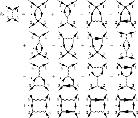
Figure 5: Diagrammatic representation of contributions to the flow of $V^{\rm PH,\Lambda}$. The dot denotes a $\Lambda$-derivative acting on the product of the two fermionic propagators.

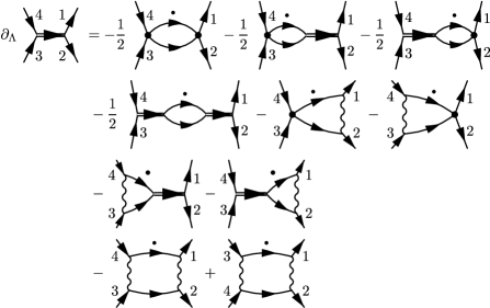
Figure 6: Diagrammatic representation of contributions to the flow of $V^{\rm PP,\Lambda}$.

Note that all diagrams are one-particle irreducible, that is, they cannot be cut by cutting a single fermionic propagator line. Some of them can be cut by cutting an interaction line, but these lines do not correspond to particle propagators, since the interaction is not represented by bosonic fields in our purely fermionic RG.

V Random phase approximation

To gain insight into the singularity structure of the Nambu vertex it is instructive to consider the random phase approximation (RPA) before analyzing the full set of flow equations. In the conventional formulation the RPA corresponds to a summation of all (direct) particle-hole ladder contributions to the Nambu vertex with bare interactions and mean-field propagators. The self-energy is obtained from the usual mean-field equation, that is, self-consistent first order perturbation theory. In the channel decomposed functional RG framework derived in Sec. IV, the RPA is equivalent to the approximation

$$\Gamma^{(4)\Lambda}_{s_{1}s_{2}s_{3}s_{4}}(k,k^{\prime};q)=U_{s_{1}s_{2}s_{3}s_{4}}(k,k^{\prime};q)+V^{\rm PH,\Lambda}_{s_{1}s_{2}s_{3}s_{4}}(k,k^{\prime};q)\;,$$ (63)

that is, the crossed particle-hole and particle-particle channels are discarded. Throughout this section we parametrize the momentum variables $k_{1},k_{2},k_{3},k_{4}$ as $k_{1}=k+\frac{q}{2}$, $k_{2}=k^{\prime}-\frac{q}{2}$, $k_{3}=k^{\prime}+\frac{q}{2}$, and $k_{4}=k-\frac{q}{2}$. The flow equation (51) for $V^{\rm PH,\Lambda}$ can then be formally integrated to obtain an integral equation which, expressed in term of $\Gamma^{(4)\Lambda}$, reads

$$\Gamma^{(4)\Lambda}_{s_{1}s_{2}s_{3}s_{4}}(k,k^{\prime};q) = U_{s_{1}s_{2}s_{3}s_{4}}(k,k^{\prime};q)$$ (64)

$$+ \sum_{p}\sum_{s^{\prime}_{i}}U_{s_{1}s^{\prime}_{2}s^{\prime}_{3}s_{4}}(k,p;q)\,G^{\Lambda}_{s^{\prime}_{1}s^{\prime}_{2}}(p-{\textstyle\frac{q}{2}})G^{\Lambda}_{s^{\prime}_{3}s^{\prime}_{4}}(p+{\textstyle\frac{q}{2}})\,\Gamma^{(4)\Lambda}_{s^{\prime}_{4}s_{2}s_{3}s^{\prime}_{1}}(p,k^{\prime};q)\;.\hskip 28.45274pt$$

This is the familiar Bethe-Salpeter-type equation corresponding to a summation of (Nambu) particle-hole ladders. Using this equation, the flow equation for the self-energy Eq. (9) can also be integrated, yielding the usual mean-field equation

$$\Sigma^{\Lambda}_{s_{1}s_{2}}=\sum_{k^{\prime}}\sum_{s^{\prime}_{1},s^{\prime}_{2}}U_{s_{1}s^{\prime}_{1}s^{\prime}_{2}s_{2}}(k,k^{\prime};0)\,G^{\Lambda}_{s^{\prime}_{2}s^{\prime}_{1}}(k^{\prime})\;.$$ (65)

The integral equation (64) can be written in matrix form such that Nambu index sums correspond to matrix products. In particular, choosing the Pauli matrix basis described in Appendix A, one obtains

$$\tilde{\bf\Gamma}^{(4)\Lambda}(k,k^{\prime};q)=\tilde{\bf U}(k,k^{\prime};q)+\sum_{p}\tilde{\bf U}(k,p;q)\,\tilde{\bf L}^{\Lambda}(p;q)\,\tilde{\bf\Gamma}^{(4)\Lambda}(p,k^{\prime};q)\;,$$ (66)

where the components of $\tilde{\bf L}^{\Lambda}(p;q)$ are given by

$$\tilde{L}^{\Lambda}_{jj^{\prime}}(p;q)=\frac{1}{2}\sum_{s_{i}}\tau^{(j)}_{s_{4}s_{1}}\tau^{(j^{\prime})}_{s_{3}s_{2}}\,G^{\Lambda}_{s_{2}s_{4}}(p-{\textstyle\frac{q}{2}})G^{\Lambda}_{s_{1}s_{3}}(p+{\textstyle\frac{q}{2}})\;.$$ (67)

For a spin-rotation invariant system, the bare interaction can be written in the form

$${\cal U}[\psi,\bar{\psi}] = \frac{1}{2}\,\sum_{k,k^{\prime},q}C^{(0)}_{kk^{\prime}}(q)\sum_{\sigma,\sigma^{\prime}}\bar{\psi}_{k+q/2,\sigma}\bar{\psi}_{k^{\prime}-q/2,\sigma^{\prime}}\psi_{k^{\prime}+q/2,\sigma^{\prime}}\psi_{k-q/2,\sigma}$$ (68)

$$+ \frac{1}{2}\,\sum_{k,k^{\prime},q}M^{(0)}_{kk^{\prime}}(q)\sum_{\sigma_{i}}\vec{\tau}_{\sigma_{1}\sigma_{4}}\cdot\vec{\tau}_{\sigma_{2}\sigma_{3}}\,\bar{\psi}_{k+q/2,\sigma_{1}}\bar{\psi}_{k^{\prime}-q/2,\sigma_{2}}\psi_{k^{\prime}+q/2,\sigma_{3}}\psi_{k-q/2,\sigma_{4}}$$

$$+ \frac{1}{2}\,\sum_{k,k^{\prime},q}\,P^{(0)}_{kk^{\prime}}(q)\sum_{\sigma,\sigma^{\prime}}\bar{\psi}_{q/2+k,\sigma}\bar{\psi}_{q/2-k,\sigma^{\prime}}\psi_{q/2-k^{\prime},\sigma^{\prime}}\psi_{q/2+k^{\prime},\sigma}\;,\hskip 14.22636pt$$

which is analogous to the decomposition of the fluctuation contributions in Eq. (31). In the special case where the bare coupling functions $C^{(0)}_{kk^{\prime}}(q)$, $M^{(0)}_{kk^{\prime}}(q)$, and $P^{(0)}_{kk^{\prime}}(q)$ are non-zero only for $q=0$, this becomes the reduced BCS and forward scattering interaction of the model discussed in detail in Ref. eberlein10, . In that case the mean-field equation for the self-energy is exact, and the Bethe-Salpeter equation yields the exact vertex $\Gamma^{(4)\Lambda}_{s_{1}s_{2}s_{3}s_{4}}(k,k^{\prime};q=0)$.

For an explicit evaluation of the RPA vertex we assume separable interactions

$$C^{(0)}_{kk^{\prime}}(q) = C^{(0)}(q)f_{c}(k)f_{c}(k^{\prime})\;,$$

$$M^{(0)}_{kk^{\prime}}(q) = M^{(0)}(q)f_{m}(k)f_{m}(k^{\prime})\;,$$

$$P^{(0)}_{kk^{\prime}}(q) = P^{(0)}(q)f_{p}(k)f_{p}(k^{\prime})\;,$$ (69)

with symmetric (under $k\mapsto-k$) form factors, and a bare gap function $\Delta_{0}(k)=\Delta_{0}f_{p}(k)$ with the same form factor as the pairing interaction. The coupling functions contributing to ${\bf V}^{\rm PH,\Lambda}$, see Eq. (53), then also factorize:

$$C^{\Lambda}_{kk^{\prime}}(q) = C^{\Lambda}(q)f_{c}(k)f_{c}(k^{\prime})\;,$$

$$M^{\Lambda}_{kk^{\prime}}(q) = M^{\Lambda}(q)f_{m}(k)f_{m}(k^{\prime})\;,$$

$$P^{\Lambda}_{kk^{\prime}}(q) = P^{\Lambda}(q)f_{p}(k)f_{p}(k^{\prime})\;,$$

$$W^{\Lambda}_{kk^{\prime}}(q) = W^{\Lambda}(q)f_{p}(k)f_{p}(k^{\prime})\;,$$

$$X^{\Lambda}_{kk^{\prime}}(q) = X^{\Lambda}(q)f_{c}(k)f_{p}(k^{\prime})\;,$$ (70)

and the gap function has the form

$$\Delta^{\Lambda}(k)=\Delta^{\Lambda}f_{p}(k)\;.$$ (71)

The vertex assumes a particularly simple form in the Pauli matrix basis, namely

$$\tilde{\bf\Gamma}^{(4)\Lambda}(k,k^{\prime};q)=\tilde{\bf f}(k)\,\tilde{\bf\Gamma}^{(4)\Lambda}(q)\,\tilde{\bf f}(k^{\prime})\;,$$ (72)

where $\tilde{\bf f}(k)$ is the diagonal matrix

$$\tilde{\bf f}(k)={\rm diag}[f_{m}(k),f_{p}(k),f_{p}(k),f_{c}(k)]\;,$$ (73)

and

$$\tilde{\bf\Gamma}^{(4)\Lambda}(q)=\tilde{\bf U}(q)+\tilde{\bf V}^{\rm PH,\Lambda}(q)\;,$$ (74)

with

$$\tilde{\bf U}(q)=\left(\begin{array}[]{cccc}2M^{(0)}(q)&0&0&0\\ 0&P^{(0)}(q)&0&0\\ 0&0&P^{(0)}(q)&0\\ 0&0&0&2C^{(0)}(q)\end{array}\right)$$ (75)

and

$$\tilde{\bf V}^{\rm PH,\Lambda}(q)=\left(\begin{array}[]{cccc}2M^{\Lambda}(q)&0&0&0\\ 0&A^{\Lambda}(q)&P^{\prime\prime\Lambda}(q)&2X^{\prime\Lambda}(q)\\ 0&-P^{\prime\prime\Lambda}(q)&\Phi^{\Lambda}(q)&-2X^{\prime\prime\Lambda}(q)\\ 0&2X^{\prime\Lambda}(q)&2X^{\prime\prime\Lambda}(q)&2C^{\Lambda}(q)\end{array}\right)\;.$$ (76)

Here $A^{\Lambda}(q)=P^{\prime\Lambda}(q)+W^{\prime\Lambda}(q)$ and $\Phi^{\Lambda}(q)=P^{\prime\Lambda}(q)-W^{\prime\Lambda}(q)$. Primes denote real parts and double primes imaginary parts. At $q_{0}=0$ all imaginary parts vanish. For $q=0$ the above matrix simplifies to the vertex previously obtained for the reduced BCS and forward scattering model, eberlein10 in a slightly different basis yielding some sign changes.

Inserting the factorized form of the vertex into the Bethe-Salpeter equation Eq. (66), one obtains a linear algebraic equation for $\tilde{\bf\Gamma}^{(4)\Lambda}(q)$,

$$\tilde{\bf\Gamma}^{(4)\Lambda}(q)=\tilde{\bf U}(q)+\tilde{\bf U}(q)\,\tilde{\bf L}^{\Lambda}(q)\,\tilde{\bf\Gamma}^{(4)\Lambda}(q)\;,$$ (77)

where

$$\tilde{\bf L}^{\Lambda}(q)=\sum_{p}\tilde{\bf f}(p)\tilde{\bf L}^{\Lambda}(p;q)\tilde{\bf f}(p)=\left(\begin{array}[]{cccc}\tilde{L}_{m}^{\Lambda}(q)&0&0&0\\ 0&\tilde{L}_{a}^{\Lambda}(q)&\tilde{L}_{p}^{\prime\prime\Lambda}(q)&\tilde{L}_{x}^{\prime\Lambda}(q)\\ 0&-\tilde{L}_{p}^{\prime\prime\Lambda}(q)&\tilde{L}_{\phi}^{\Lambda}(q)&-\tilde{L}_{x}^{\prime\prime\Lambda}(q)\\ 0&\tilde{L}_{x}^{\prime\Lambda}(q)&\tilde{L}_{x}^{\prime\prime\Lambda}(q)&\tilde{L}_{c}^{\Lambda}(q)\end{array}\right)\;.$$ (78)

The matrix elements $\tilde{L}^{\Lambda}_{0j}$ and $\tilde{L}^{\Lambda}_{j0}$ with $j=1,2,3$ vanish for symmetric form factors. The other matrix elements are given by

$$\tilde{L}_{c}^{\Lambda}(q) = \sum_{p}\left[G^{\Lambda}(p-{\textstyle\frac{q}{2}})G^{\Lambda}(p+{\textstyle\frac{q}{2}})-F^{\Lambda}(p-{\textstyle\frac{q}{2}})F^{\Lambda}(p+{\textstyle\frac{q}{2}})\right]f_{c}^{2}(p)\;,$$

$$\tilde{L}_{m}^{\Lambda}(q) = \sum_{p}\left[G^{\Lambda}(p-{\textstyle\frac{q}{2}})G^{\Lambda}(p+{\textstyle\frac{q}{2}})+F^{\Lambda}(p-{\textstyle\frac{q}{2}})F^{\Lambda}(p+{\textstyle\frac{q}{2}})\right]f_{m}^{2}(p)\;,$$

$$\tilde{L}_{a}^{\Lambda}(q) = -\sum_{p}\left\{{\rm Re}\left[G^{\Lambda}(p+{\textstyle\frac{q}{2}})G^{\Lambda}(-p+{\textstyle\frac{q}{2}})\right]-F^{\Lambda}(p-{\textstyle\frac{q}{2}})F^{\Lambda}(p+{\textstyle\frac{q}{2}})\right\}f_{p}^{2}(p)\;,$$

$$\tilde{L}_{\phi}^{\Lambda}(q) = -\sum_{p}\left\{{\rm Re}\left[G^{\Lambda}(p+{\textstyle\frac{q}{2}})G^{\Lambda}(-p+{\textstyle\frac{q}{2}})\right]+F^{\Lambda}(p-{\textstyle\frac{q}{2}})F^{\Lambda}(p+{\textstyle\frac{q}{2}})\right\}f_{p}^{2}(p)\;,$$

$$\tilde{L}_{p}^{\prime\prime\Lambda}(q) = -\sum_{p}{\rm Im}\left[G^{\Lambda}(p+{\textstyle\frac{q}{2}})G^{\Lambda}(-p+{\textstyle\frac{q}{2}})\right]f_{p}^{2}(p)\;,$$

$$\tilde{L}_{x}^{\prime\Lambda}(q) = 2\sum_{p}{\rm Re}\left[G^{\Lambda}(p-{\textstyle\frac{q}{2}})F^{\Lambda}(p+{\textstyle\frac{q}{2}})\right]f_{c}(p)f_{p}(p)\;,$$

$$\tilde{L}_{x}^{\prime\prime\Lambda}(q) = 2\sum_{p}{\rm Im}\left[G^{\Lambda}(p-{\textstyle\frac{q}{2}})F^{\Lambda}(p+{\textstyle\frac{q}{2}})\right]f_{c}(p)f_{p}(p)\;.$$ (79)

The system of linear equations Eq. (77) can be solved explicitly. The magnetic coupling function is decoupled from the others, so that $M^{(0)}(q)+M^{\Lambda}(q)=\{[M^{(0)}(q)]^{-1}-\tilde{L}_{m}^{\Lambda}(q)\}^{-1}$. Solving for the other coupling functions amounts to solving a linear $3\times 3$ system. We do not write the explicit expressions here, but discuss only the singularity structure of the coupling functions. Singularities arise because the determinant $d^{\Lambda}(q)={\rm det}[{\bf 1}-\tilde{\bf U}(q)\tilde{\bf L}^{\Lambda}(q)]$ vanishes at $q=0$ for $\Delta_{0}\to 0$, if $\Delta^{\Lambda}(k)$ remains finite, that is, in case of spontaneous symmetry breaking. For $q=0$, the explicit solution for the coupling functions and their behavior for $\Delta_{0}\to 0$ was discussed in detail in Ref. eberlein10, . For small $q\neq 0$, one can expand $d(q)=d^{\Lambda=0}(q)=d_{0}+d_{1}q_{0}^{2}+d_{2}{\bf q}^{2}+\dots$, where $d_{0}\propto\Delta_{0}$ for small $\Delta_{0}$, while $d_{1}$ and $d_{2}$ remain finite for $\Delta_{0}\to 0$. Expanding all coefficients to leading order in $q_{0}$ and ${\bf q}$, one obtains the singular coupling functions

$$\Phi(q) \propto -\frac{1}{d_{0}+d_{1}q_{0}^{2}+d_{2}{\bf q}^{2}}\;,$$

$$P^{\prime\prime}(q) \propto -\frac{q_{0}}{d_{0}+d_{1}q_{0}^{2}+d_{2}{\bf q}^{2}}\;,$$

$$X^{\prime\prime}(q) \propto -\frac{q_{0}}{d_{0}+d_{1}q_{0}^{2}+d_{2}{\bf q}^{2}}$$ (80)

for $\Lambda=0$. The other coupling functions, $C^{\Lambda}(q)$, $M^{\Lambda}(q)$, $A^{\Lambda}(q)$, and the real part of $X^{\Lambda}(q)$ remain finite for $\Lambda\to 0$, $\Delta_{0}\to 0$, $q\to 0$.

The divergence of the vertex in the phase fluctuation channel represented by the coupling function $\Phi^{\Lambda}(q)$ reflects the Goldstone mode associated with the spontaneous breaking of the $U(1)$ symmetry. The Goldstone theorem, which guarantees the existence of this mode, is obviously respected by the RPA. A less familiar interesting result of the above calculation is the divergence of the (3+1)-interaction represented by the coupling function $X^{\Lambda}(q)$. At $q=0$ this interaction describes pair annihilation (or creation) combined with a forward scattering process.

VI Attractive Hubbard model

In this section we compute the flow of the Nambu vertex and the gap function for the two-dimensional attractive Hubbard model as a prototype of a spin-singlet superfluid.

The Hubbard model describes interacting spin-$\frac{1}{2}$ lattice fermions with the Hamiltonian

$$H=\sum_{{\bf i},{\bf j}}t_{{\bf i}{\bf j}}c^{{\dagger}}_{{\bf i}\sigma}c_{{\bf j}\sigma}+U\sum_{{\bf j}}n_{{\bf j}\uparrow}n_{{\bf j}\downarrow}\;,$$ (81)

where $c^{{\dagger}}_{{\bf i}\sigma}$ and $c_{{\bf i}\sigma}$ are creation and annihilation operators for fermions with spin orientation $\sigma$ on a lattice site ${\bf i}$. For the attractive Hubbard model the interaction parameter $U$ is negative. The hopping matrix $t_{{\bf i}{\bf j}}$ is usually short-ranged. We consider the case of nearest and next-to-nearest neighbor hopping on a square lattice, with amplitudes $-t$ and $-t^{\prime}$, respectively, yielding a dispersion relation of the form

$$\epsilon({\bf k})=-2t\left(\cos k_{x}+\cos k_{y}\right)-4t^{\prime}\cos k_{x}\cos k_{y}\;.$$ (82)

The ground state of the attractive Hubbard model is a spin-singlet $s$-wave superfluid at any filling factor.micnas90 For $t^{\prime}=0$ the superfluid order is degenerate with a charge density wave at half-filling (only). The attractive Hubbard model has been studied already in several works both at zero and finite temperature by resummed perturbation theory (mostly T-matrix),fresard92 ; pedersen97 ; letz98 ; keller99 quantum Monte Carlo (QMC) methods,randeria92 ; santos94 ; singer96 and dynamical mean-field theory.keller01 ; capone02

VI.1 Regularization and counterterm

The renormalization group flow is governed by the scale dependence of the regularized bare propagator, which we choose to be of the following form

$$\left[{\bf G}_{0}^{\Lambda}(k)\right]^{-1}=\left(\begin{array}[]{cc}ik_{0}-\xi({\bf k})-\delta\xi^{\Lambda}({\bf k})+R^{\Lambda}(k_{0})&\Delta_{0}\\ \Delta_{0}&ik_{0}+\xi({\bf k})+\delta\xi^{\Lambda}({\bf k})+R^{\Lambda}(k_{0})\end{array}\right)\;,$$ (83)

with $\xi({\bf k})=\epsilon({\bf k})-\mu$. The regulator function

$$R^{\Lambda}(k_{0})=i\,{\rm sgn}(k_{0})\sqrt{k_{0}^{2}+\Lambda^{2}}-ik_{0}$$ (84)

replaces frequencies $k_{0}$ with $|k_{0}|\ll\Lambda$ by ${\rm sgn}(k_{0})\Lambda$ and thus regularizes the Fermi surface singularity of the bare fermionic propagator. The (real) bare gap $\Delta_{0}$ induces symmetry breaking and regularizes the Goldstone mode singularity forming in the effective interaction below the critical scale $\Lambda_{c}$. Instead of linking the flow of $\Delta_{0}$ to the fermionic cutoff scale $\Lambda$ by defining a $\Lambda$-dependent $\Delta_{0}^{\Lambda}$, we found it more convenient to keep $\Delta_{0}$ fixed until $\Lambda$ has decreased to $0$, and send $\Delta_{0}$ to zero afterwards. The equations for the latter flow are obtained simply by replacing $\Lambda$-derivatives by derivatives with respect to $\Delta_{0}$. The counterterm $\delta\xi^{\Lambda}({\bf k})$ is linked to the normal component of the self-energy by the condition

$$\frac{d}{d\Lambda}\left[\delta\xi^{\Lambda}({\bf k})+\Sigma^{\Lambda}(0,{\bf k})\right]=0\;,$$ (85)

such that the Fermi surface remains fixed during the flow. Since there is a contribution proportional to $\partial_{\Lambda}\delta\xi^{\Lambda}$ to the scale derivative of $\Sigma^{\Lambda}$, solving Eq. (85) for $\partial_{\Lambda}\delta\xi^{\Lambda}$ amounts to solving a linear integral equation.

VI.2 Parametrization

We now specify the approximate parametrization of the self-energy and the interaction vertex. Due to the local bare interaction and the pairing instability occurring in the $s$-wave channel, the momentum dependence of the normal and anomalous self-energy can be expected to be weak, at least at weak coupling. Perturbation theory neumayr03 and previous functional RG calculations gersch08 showed that this is indeed the case. We therefore discard the momentum dependence of the self-energy, keeping however the frequency dependence. The latter is treated numerically by discretizing $\Sigma^{\Lambda}(k_{0})$ and $\Delta^{\Lambda}(k_{0})$ on a suitable grid. The counterterm $\delta\xi^{\Lambda}$ is then also momentum independent and can be interpreted as a shift of the chemical potential.

The interaction vertex is fully described by the coupling functions $C^{\Lambda}_{kk^{\prime}}(q)$ etc. introduced in Sec. IV, where singular momentum and frequency dependences have been isolated in one variable $q$. We now approximate these functions by the following ansatz:

$$C^{\Lambda}_{kk^{\prime}}(q) = C^{\Lambda}(q)\,g^{\Lambda}_{c}(k_{0})\,g^{\Lambda}_{c}(k^{\prime}_{0})\;,$$

$$M^{\Lambda}_{kk^{\prime}}(q) = M^{\Lambda}(q)\,g^{\Lambda}_{m}(k_{0})\,g^{\Lambda}_{m}(k^{\prime}_{0})\;,$$

$$A^{\Lambda}_{kk^{\prime}}(q) = A^{\Lambda}(q)\,g^{\Lambda}_{a}(k_{0})\,g^{\Lambda}_{a}(k^{\prime}_{0})\;,$$

$$\Phi^{\Lambda}_{kk^{\prime}}(q) = \Phi^{\Lambda}(q)\,g^{\Lambda}_{\phi}(k_{0})\,g^{\Lambda}_{\phi}(k^{\prime}_{0})\;,$$

$$P^{\prime\prime\Lambda}_{kk^{\prime}}(q) = P^{\prime\prime\Lambda}(q)\,g^{\Lambda}_{\phi}(k_{0})\,g^{\Lambda}_{\phi}(k^{\prime}_{0})\;,$$

$$X^{\prime\Lambda}_{kk^{\prime}}(q) = X^{\prime\Lambda}(q)\,g^{\Lambda}_{c}(k_{0})\,g^{\Lambda}_{a}(k^{\prime}_{0})\;,$$

$$X^{\prime\prime\Lambda}_{kk^{\prime}}(q) = X^{\prime\prime\Lambda}(q)\,g^{\Lambda}_{c}(k_{0})\,g^{\Lambda}_{\phi}(k^{\prime}_{0})\;.$$ (86)

The vertex thus assumes the form of a collection of boson-mediated interactions with bosonic propagators coupled to the fermions via fermion-boson vertices $g^{\Lambda}$. The latter are normalized to one at zero frequency ($k_{0}=0$). The momentum dependence on ${\bf k}$ and ${\bf k}^{\prime}$ has thus been neglected, and the dependence on $k_{0}$ and $k^{\prime}_{0}$ has been factorized. For the attractive Hubbard model, dependences on $k$ and $k^{\prime}$ are generated only at order $U^{3}$, and can thus be expected to be weak at least at weak coupling. Neglecting the dependence on ${\bf k}$ and ${\bf k}^{\prime}$ implies a restriction to $s$-wave symmetry in charge, magnetic and pairing channels. As a consequence, all triplet components vanish, such that $A^{\Lambda}_{kk^{\prime}}(q)=A^{S,\Lambda}_{kk^{\prime}}(q)$, $\Phi^{\Lambda}_{kk^{\prime}}(q)=\Phi^{S,\Lambda}_{kk^{\prime}}(q)$, and $X^{\Lambda}_{kk^{\prime}}(q)=X^{S,\Lambda}_{kk^{\prime}}(q)$, and in the matrix ${\bf V}^{\rm PP,\Lambda}$, Eq. (57), only four elements are non-zero. Compared to an exact decomposition of the coupling functions as in Eqs. (60) and (62), the sum over basis functions is replaced by just one term in the above ansatz. Due to time-reversal and exchange symmetries there is no contribution to $W^{\prime\prime\Lambda}_{kk^{\prime}}(q)$ of that form. We have allowed for four distinct fermion-boson vertices $g^{\Lambda}_{c}$, $g^{\Lambda}_{m}$, $g^{\Lambda}_{a}$, and $g^{\Lambda}_{\phi}$. The factorization of the coupling functions is similar to the factorization Eq. (V) obtained for separable interactions in RPA. Instead of parametrizing the fermion-boson vertices in the pairing channel by a single function $g^{\Lambda}_{p}$, we now distinguish between $g^{\Lambda}_{a}$ and $g^{\Lambda}_{\phi}$. It turns out that they differ only slightly. The imaginary part of the pairing coupling function $P^{\prime\prime\Lambda}_{kk^{\prime}}(q)$ has little impact on the flow. Instead of introducing another fermion-boson vertex for that quantity, we approximate its dependence on $k_{0}$ and $k^{\prime}_{0}$ by $g^{\Lambda}_{\phi}$. The frequency dependence of the fermion-boson vertices $g^{\Lambda}(k_{0})$ is treated numerically by discretization.

The parametrization of the “boson propagators” $C^{\Lambda}(q)$ etc. requires special care, to capture the singularities. We first consider the amplitude and phase channel. For small $q$ the functions $A^{\Lambda}(q)$ and $\Phi^{\Lambda}(q)$ behave as $[A^{\Lambda}(q)]^{-1}=-m^{\Lambda}_{a}-Z^{\Lambda}_{a}{\bf q}^{2}-\bar{Z}^{\Lambda}_{a}q_{0}^{2}+\dots$ and $[\Phi^{\Lambda}(q)]^{-1}=-m^{\Lambda}_{\phi}-Z^{\Lambda}_{\phi}{\bf q}^{2}-\bar{Z}^{\Lambda}_{\phi}q_{0}^{2}+\dots$, where $m^{\Lambda}_{\phi}\to 0$ for $\Lambda<\Lambda_{c}$, $\Delta_{0}\to 0$. Actually the regulator function can also generate contributions of order $|q_{0}|$, which disappear again as $\Lambda\to 0$. To deal with this technical complication, and to achieve an accurate parametrization also at larger values of $q_{0}$ and ${\bf q}$, we parametrize $A^{\Lambda}$ and $\Phi^{\Lambda}$ by two scale-dependent functions,

$$\left[A^{\Lambda}(q)\right]^{-1} = -m^{\Lambda}_{a}(q_{0})-e^{\Lambda}_{a}({\bf q})\;,$$

$$\left[\Phi^{\Lambda}(q)\right]^{-1} = -m^{\Lambda}_{\phi}(q_{0})-e^{\Lambda}_{\phi}({\bf q})\;,$$ (87)

where $e^{\Lambda}_{a}({\bf 0})=e^{\Lambda}_{\phi}({\bf 0})=0$. The (discretized) momentum and frequency dependences of these functions are determined from the flow. The above ansatz with functions of one ($q_{0}$) and two (${\bf q}=(q_{x},q_{y})$) variables reduces the numerical effort compared to a discretization of an arbitrary function of $q=(q_{0},q_{x},q_{y})$. Tests within RPA indicate that it describes the full functions sufficiently well. In particular, the behavior at small $q_{0}$ and small ${\bf q}$ is captured correctly. The imaginary parts $P^{\prime\prime\Lambda}(q)$ and $X^{\prime\prime\Lambda}(q)$ are odd functions of $q_{0}$. This and the expected singularity structure [see Eq. (V)] motivate the ansatz

$$P^{\prime\prime\Lambda}(q) = -\frac{q_{0}}{m^{\Lambda}_{p^{\prime\prime}}(q_{0})+e^{\Lambda}_{p^{\prime\prime}}({\bf q})}\;,$$

$$X^{\prime\prime\Lambda}(q) = -\frac{q_{0}}{m^{\Lambda}_{x^{\prime\prime}}(q_{0})+e^{\Lambda}_{x^{\prime\prime}}({\bf q})}\;.$$ (88)

The parametrization of $C^{\Lambda}(q)$, $M^{\Lambda}(q)$ and $X^{\prime\Lambda}(q)$ is slightly more complicated, because at small ${\bf q}$ these functions cannot be represented as a sum of a frequency and a momentum dependent function. We therefore distinguish the cases $|{\bf q}|<q_{\rm max}$ and $|{\bf q}|>q_{\rm max}$ with a suitably chosen $q_{\rm max}$. For $|{\bf q}|>q_{\rm max}$ we make an additive ansatz analogous to Eq. (VI.2),

$$\left[C^{\Lambda}(q)\right]^{-1} = -m^{\Lambda}_{c}(q_{0})-e^{\Lambda}_{c}({\bf q})\;,$$

$$\left[M^{\Lambda}(q)\right]^{-1} = -m^{\Lambda}_{m}(q_{0})-e^{\Lambda}_{m}({\bf q})\;,$$

$$\left[X^{\prime\Lambda}(q)\right]^{-1} = -m^{\Lambda}_{x^{\prime}}(q_{0})-e^{\Lambda}_{x^{\prime}}({\bf q})\;.$$ (89)

For small ${\bf q}$, the ${\bf q}$-dependence is increasingly isotropic, except for the special case where the Fermi surface touches van Hove points (which we exclude). Hence, for $|{\bf q}|<q_{\rm max}$ we approximate the momentum dependence as isotropic,

$$C^{\Lambda}(q) = C^{\Lambda}(q_{0},|{\bf q}|)\;,$$

$$M^{\Lambda}(q) = M^{\Lambda}(q_{0},|{\bf q}|)\;,$$

$$X^{\prime\Lambda}(q) = X^{\prime\Lambda}(q_{0},|{\bf q}|)\;,$$ (90)

reducing the number of variables again to two. To avoid a discontinuity at $q_{\rm max}$, we connect the two regimes in momentum space by a smooth partition of unity instead of step functions.

VI.3 Flow equations

The flow equations for the scale-dependent functions parametrizing the self-energy and interaction vertex are obtained by projecting the flow equations for the self-energy and the coupling functions on the simplified ansatz. Dependences on the fermionic momenta ${\bf k}$, ${\bf k}^{\prime}$ generated by the flow are eliminated by a Fermi surface average (but not the ${\bf q}$-dependence, of course). This corresponds to keeping only the leading (in power-counting) term in an expansion around the Fermi surface, and averaging over the momentum dependence along the Fermi surface, which is in line with the pure $s$-wave ansatz for the interactions.

For the self-energy, we project on the momentum-independent ansatz by averaging the flow Eq. (9) over the Fermi surface as follows:

$$\frac{d}{d\Lambda}{\bf\Sigma}^{\Lambda}(k_{0})=\langle{\bf rhs}^{\Lambda}(k_{0},{\bf k})\rangle_{{\bf k}\in{\rm FS}}\;,$$ (91)

where ${\bf rhs}^{\Lambda}(k_{0},{\bf k})$ stands for the right hand side of the flow equation (in Nambu matrix form), and $\langle\dots\rangle_{{\bf k}\in{\rm FS}}$ denotes a Fermi surface average. Momentum dependences of the self-energy perpendicular to the Fermi surface are marginal in power-counting shankar94 and lead to a (finite) renormalization of the Fermi velocity. However, they are quantitatively small in the attractive Hubbard model, at least at weak coupling and away from van Hove points, and have thus little influence on our results.

The flow equations for the coupling functions $C^{\Lambda}_{kk^{\prime}}(q),\dots,X^{\Lambda}_{kk^{\prime}}(q)$ were derived in Sec. IV. Inserting the ansatz for the interaction vertex on the right hand side of these equations yields several terms which can be represented by Feynman diagrams of the form plotted in Fig. 5. We recall that the point-like vertex represents the bare (here Hubbard) interaction, the wiggly line any coupling function contributing to ${\bf V}^{\rm PH,\Lambda}$, and the double line coupling functions appearing in ${\bf V}^{\rm PP,\Lambda}$ (only $M^{\Lambda}_{kk^{\prime}}(q)$ in the absence of triplet terms). Note that the terms in Fig. 6 are redundant since the complete set of coupling functions is already captured by ${\bf V}^{\rm PH,\Lambda}$. The Nambu index sums on the right hand side of the flow equation for the coupling functions can be transformed to a more convenient form by representing the vertex and the propagator product in the Pauli matrix basis defined in Appendix A and used already in Sec. V.

Some of the contributions, having the form of vertex corrections or box diagrams, generate dependences on ${\bf k}$ and ${\bf k}^{\prime}$ which are not allowed for in our ansatz. These dependences are projected out by a symmetrized Fermi surface average. We discuss the procedure for the charge coupling function as a prototypical example, which can be extended directly to all other cases. The flow of the projected charge coupling function is given by

$$\frac{d}{d\Lambda}\left[C^{\Lambda}(q)\,g^{\Lambda}_{c}(k_{0})\,g^{\Lambda}_{c}(k^{\prime}_{0})\right] = \langle{\rm rhs}^{\Lambda}(k,k^{\prime};q)\rangle_{{\bf k}\pm\frac{{\bf q}}{2},{\bf k}^{\prime}\pm\frac{{\bf q}}{2}\in{\rm FS}}$$ (92)

$$\equiv \overline{\rm rhs}^{\Lambda}(k_{0},k^{\prime}_{0};q)\;,$$

where ${\rm rhs}^{\Lambda}(k,k^{\prime};q)$ denotes the complete right hand side of the flow equation for $C^{\Lambda}_{kk^{\prime}}$, Eq. (33), and

$$\langle\dots\rangle_{{\bf k}\pm\frac{{\bf q}}{2},{\bf k}^{\prime}\pm\frac{{\bf q}}{2}\in{\rm FS}}=\frac{1}{4}\sum_{\epsilon,\epsilon^{\prime}=\pm 1}\langle\dots\rangle_{{\bf k}+\epsilon\frac{{\bf q}}{2},{\bf k}^{\prime}+\epsilon^{\prime}\frac{{\bf q}}{2}\in{\rm FS}}$$ (93)

is a symmetrized Fermi surface average. The latter averages the four possible ways of integrating ${\bf k}$ and ${\bf k}^{\prime}$ under the constraint that two of the four external momenta ${\bf k}\pm\frac{{\bf q}}{2}$ and ${\bf k}^{\prime}\pm\frac{{\bf q}}{2}$ of the vertex lie on the Fermi surface. For ${\bf q}={\bf 0}$, corresponding to the forward scattering and Cooper channels, this becomes a Fermi surface average with all four momenta on the Fermi surface. For ${\bf q}\neq{\bf 0}$, the set of momenta ${\bf k}$ satisfying both ${\bf k}+\frac{{\bf q}}{2}\in{\rm FS}$ and ${\bf k}-\frac{{\bf q}}{2}\in{\rm FS}$ is limited to few points, except for special nesting vectors in case of a nested Fermi surface. The Fermi surface average picks up the $s$-wave component of the dominant processes near the Fermi surface. Indeed, the momentum dependence perpendicular to the Fermi surface is irrelevant in power-counting.shankar94 Note, however, that we do not discard the dependence on ${\bf q}$. That dependence becomes important due to the formation of singularities, which invalidate the weak-coupling power-counting.

The projection on the form factors in the channel decomposition could also be carried out by integration over the entire Brillouin zone.husemann09 ; husemann12 However, for our simple ansatz with only one (momentum-independent) form factor it is better to approximate the vertex by its Fermi surface average instead of a Brillouin zone average, to capture the dominant contributions at low energy scales. We checked this in some test cases by explicit comparison of different projection procedures.

The flow equation for the bosonic propagator can be extracted from Eq. (92) by setting $k_{0}=k^{\prime}_{0}=0$. Since $g^{\Lambda}_{c}(0)=1$ is independent of $\Lambda$, one obtains

$$\frac{d}{d\Lambda}C^{\Lambda}(q)=\overline{\rm rhs}^{\Lambda}(0,0;q)\;.$$ (94)

The functions $m_{c}^{\Lambda}(q_{0})$ and $e_{c}^{\Lambda}({\bf q})$ parametrizing $C^{\Lambda}(q)$ for $|{\bf q}|>q_{\rm max}$ are extracted by evaluating $[C^{\Lambda}(q)]^{-1}$ at a fixed momentum ${\bf q}^{*}$ as a function of $q_{0}$, and at fixed frequency $q_{0}=0$ as a function of ${\bf q}$, respectively. For ${\bf q}^{*}$ we choose a momentum where $C^{\Lambda}(q)$ is peaked, where it yields the largest contribution. In the charge and magnetic channel this happens typically at finite momenta connecting antipodal Fermi points ($2k_{F}$-type momenta).

The product rule for differentiation applied to the left hand side of Eq. (92) at $k^{\prime}_{0}=0$ yields the flow equation for the fermion-boson vertex,

$$\frac{d}{d\Lambda}g^{\Lambda}_{c}(k_{0})=\frac{1}{C^{\Lambda}(q)}\left[\overline{\rm rhs}^{\Lambda}(k_{0},0;q)-g^{\Lambda}_{c}(k_{0})\,\overline{\rm rhs}^{\Lambda}(0,0;q)\right]_{q=(0,{\bf q}^{*})}\;.$$ (95)

The flow equations for the other coupling functions $M^{\Lambda}_{kk^{\prime}}(q)$ etc. are projected on the ansatz in the same way. The flow of the fermion-boson vertices in the pairing channel $g^{\Lambda}_{a}(k_{0})$ and $g^{\Lambda}_{\phi}(k_{0})$ is determined as in Eq. (95), with ${\bf q}^{*}={\bf 0}$.

The initial conditions for the flow at $\Lambda_{0}=\infty$ are as follows. For the self-energy, counterterm and gap function the flow starts at $\Sigma^{\Lambda_{0}}=0$, $\delta\xi^{\Lambda_{0}}=0$, and $\Delta^{\Lambda_{0}}=\Delta_{0}$. The coupling functions are initially zero, and the fermion-boson vertices are equal to one. Note that the coupling functions do not include the bare interaction. In a numerical evaluation, the flow starts at a large finite $\Lambda_{0}$. The self-energy receives a tadpole contribution of order one in the flow from $\Lambda_{0}=\infty$ to an arbitrarily large finite $\Lambda_{0}$, yielding $\Sigma^{\Lambda_{0}}=U/2$ with corrections of order $\Lambda_{0}^{-1}$, and correspondingly $\delta\xi^{\Lambda_{0}}=-U/2$. The error of order $\Lambda_{0}^{-1}$ made by starting the flow at a (large) finite cutoff can be significantly reduced by using perturbative results at $\Lambda_{0}$ as initial conditions instead of the initial values at $\Lambda_{0}=\infty$. The coupling functions are then non-zero from the beginning such that Eq. (95) is well defined at $\Lambda_{0}$.

We conclude this section with a few words on numerical aspects. More details can be found in Ref. eberlein13, . Momentum and frequency dependences were discretized on non-equidistant grids such that the resolution is higher at smaller frequencies and momenta. The positive frequency axis and radial momentum dependences were discretized by around 30 points, and angular momentum dependences by 6 angles per quadrant in the Brillouin zone. The functional flow equations were thus replaced by a system of around 2000 non-linear ordinary differential equations with three-dimensional loop integrals on the right hand sides. The integrals were performed with an adaptive integration algorithm and the integration of the flow was performed with a third-order Runge-Kutta routine. Depending on parameters, the computation of a flow required between a day and a week on 20 CPU cores.

VI.4 Results

We now present results for the effective interactions, the normal self-energy, and the gap function as obtained from a numerical solution of the flow equations. Most of the numerical results are obtained for a small fixed external pairing field $\Delta_{0}$ chosen two to three orders of magnitude below the mean-field gap $\Delta_{\rm MF}$, but we also discuss some flows where $\Delta_{0}$ scales toward zero after the fermionic cutoff has reached $\Lambda=0$. The Ward identity following from global charge conservation is enforced at zero frequency by projecting the flow, if not stated otherwise (for details, see Sec. VI.4.3). Bare interaction strengths are chosen in the weak to moderate coupling range $|U|/t=1-4$. In the following we set the nearest-neighbor hopping amplitude $t=1$, that is, all quantities with dimension of energy are in units of $t$.

VI.4.1 Effective interactions

We begin with results for the coupling functions, which describe the various effective interaction channels contributing to the the Nambu vertex. With our sign conventions negative coupling functions correspond to attractive effective interactions in the respective channel.

The flow of effective interactions in the pairing channel is qualitatively similar to the one in RPA (see Sec. V). However, the critical scale and the size of the coupling functions is reduced by fluctuations. Typical flows for the amplitude and phase couplings at $q=0$ are shown in Fig. 7 for various choices of the external pairing field $\Delta_{0}$.

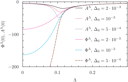
Figure 7: (Color online) Scale dependence of the amplitude and phase couplings $A^{\Lambda}$ and $\Phi^{\Lambda}$ at $q=0$ for various choices of the external pairing field $\Delta_{0}$. The Hubbard model parameters are $t^{\prime}=-0.1$, $U=-2$, $n=0.5$ (quarter-filling).

For $U=-2$ stable flows without artificial singularities could be performed for external pairing fields as small as three orders of magnitude below the size of the mean-field gap $\Delta_{\rm MF}$, with a final phase coupling $\Phi^{\Lambda=0}(0)$ proportional to $\Delta_{0}^{-1}$ within numerical accuracy, as dictated by the Ward identity. The amplitude coupling $A^{\Lambda}(0)$ has a peak around $\Lambda_{c}$, whose size increases strongly upon reducing $\Delta_{0}$, while it reaches a finite value with a negligible dependence on the external pairing field at the end of the flow.

The momentum and frequency dependence of $A^{\Lambda}(q)$ and $\Phi^{\Lambda}(q)$ around $q=0$ is shown for various choices of $\Lambda$ in Fig. 8.

     

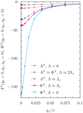
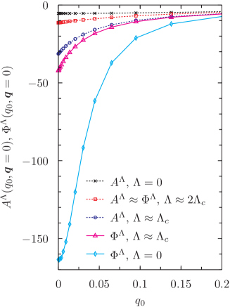
Figure 8: (Color online) Momentum dependence along the $q_{x}$-axis (left) and frequency dependence (right) of the amplitude and phase couplings $A^{\Lambda}(q)$ and $\Phi^{\Lambda}(q)$ for small momenta and frequencies at various stages of the flow. The Hubbard model parameters are the same as in Fig. 7 and $\Delta_{0}=10^{-3}$.

For small momenta, the coupling functions are isotropic functions of ${\bf q}$ with a momentum dependence proportional to ${\bf q}^{2}$, for both finite $\Lambda$ and $\Lambda=0$. The frequency dependence is linear for small $q_{0}$ at $\Lambda>0$, but essentially quadratic for $\Lambda=0$. The linear behavior at $\Lambda>0$ is caused by the frequency dependent regulator, Eq. (84), and thus disappears once the regulator has scaled to zero. The amplitude coupling $A^{\Lambda=0}(q_{0},{\bf 0})$ exhibits a tiny dip at $q_{0}=0$. Overall, the qualitative momentum and frequency dependences of the coupling functions in the pairing channel do not deviate significantly from the behavior in RPA. This is also true for the imaginary part of the pairing coupling $P^{\prime\prime\Lambda}(q)$ and the imaginary part of the anomalous (3+1)-coupling $X^{\prime\prime\Lambda}(q)$, whose singular behavior at small momenta and frequencies is well described by

$$X^{\prime\prime\Lambda=0}(q)\propto P^{\prime\prime\Lambda=0}(q)\propto-\frac{q_{0}}{\Delta_{0}+aq_{0}^{2}+b{\bf q}^{2}}\;,$$ (96)

where $a,b$ are positive constants.

The charge coupling function $C^{\Lambda}(q)$ is generally negative at all stages of the flow. It thus renormalizes the bare attraction in the charge channel given by $U$ to an enhanced total attractive interaction $U+2C^{\Lambda}(q)$. This effect is captured already in RPA. The enhancement is usually small. However, for densities near half-filling and small values of $t^{\prime}$ it becomes large at $q=(0,{\bf Q})$ with ${\bf Q}=(\pi,\pi)$. For $t^{\prime}=0$ and half-filling, $U+2C^{\Lambda}(0,{\bf Q})$ is degenerate with the pairing interaction $U+P^{\Lambda}(0,{\bf 0})$, reflecting the degeneracy of superfluidity with charge density wave order due to a particle-hole symmetry in this special case.micnas90 In Fig. 9 we show the momentum dependence of the charge coupling function in the static limit $q_{0}=0$ at the end of the flow ($\Lambda=0$) for two distinct choices of $t^{\prime}$ and $n$.

     

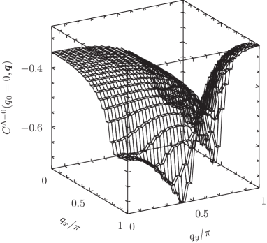
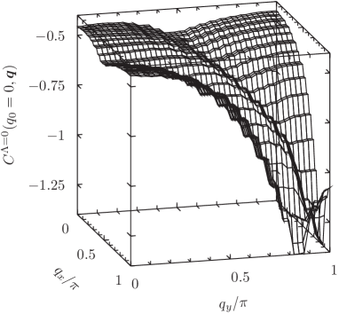
Figure 9: Momentum dependence of the static charge coupling function $C^{\Lambda=0}(0,{\bf q})$ at the end of the flow, for $t^{\prime}=-0.1$, $n=0.5$ (left) and $t^{\prime}=0$, $n=0.78$ (right). The Hubbard interaction is $U=-2$ in both cases.

The function exhibits pronounced peaks at incommensurate momenta situated at the Brillouin zone boundary. These peaks are present already in the bare polarization function (particle-hole bubble).holder12 They move toward $(\pi,\pi)$ and increase upon approaching half-filling for $t^{\prime}=0$. As a function of frequency, the size of $C^{\Lambda}(q)$ decays monotonically upon increasing $|q_{0}|$.

The magnetic coupling function $M^{\Lambda}(q)$ receives contributions beyond RPA which change its behavior qualitatively. In Fig. 10 we show its momentum dependence in the static limit $q_{0}=0$ at the end of the flow for the same choices of $t^{\prime}$ and $n$ as in Fig. 9.

     

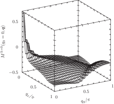
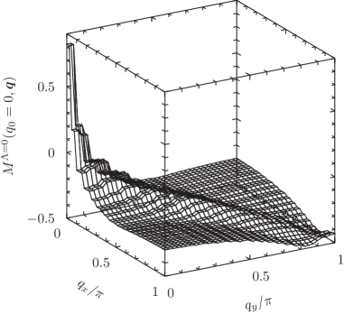
Figure 10: Momentum dependence of the static magnetic coupling function $M^{\Lambda=0}(0,{\bf q})$ at the end of the flow, for $t^{\prime}=-0.1$, $n=0.5$ (left) and $t^{\prime}=0$, $n=0.78$ (right). The Hubbard interaction is $U=-2$ in both cases.

The coupling function is negative in most of the Brillouin zone, but it develops a pronounced positive peak for small momenta ${\bf q}$. This peak is a pure fluctuation effect. In RPA, $M^{\Lambda=0}(0,{\bf 0})$ vanishes due to the pairing gap. Since the amplitude of the coupling function is small, the total interaction in the magnetic channel $-U+2M^{\Lambda=0}(q)$ is dominated by the bare Hubbard interaction and remains positive for all momenta. In Fig. 11 the frequency dependence of $M^{\Lambda}(q_{0},{\bf 0})$ is shown at various stages of the flow.

     

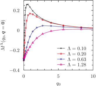
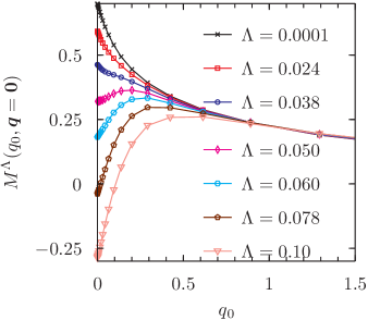
Figure 11: (Color online) Frequency dependence of the magnetic coupling function $M^{\Lambda}(q_{0},{\bf 0})$ at various stages of the flow above (left) and below (right) the critical scale for pairing. The model parameters are $t^{\prime}=-0.1$, $U=-2$, and $n=0.5$.

The positive peak at $q_{0}=0$ develops at and below the critical scale $\Lambda_{c}$ and is foreshadowed by a finite frequency peak for $\Lambda$ near $\Lambda_{c}$. The flow is non-monotonic and $M^{\Lambda}(q_{0},{\bf 0})$ exhibits a sign change for small $q_{0}$, but eventually $M^{\Lambda=0}(q_{0},{\bf 0})$ is positive for all frequencies. A similar sign change at finite $q_{0}$ and a pronounced finite frequency peak has been observed previously in the charge coupling function for the repulsive Hubbard model in the symmetric regime ($\Lambda>\Lambda_{c}$).husemann12 ; giering12

The real part of the anomalous (3+1)-coupling function $X^{\prime\Lambda}(q)$ is relatively small. Its singularity at the critical scale $\Lambda_{c}$ is considerably broadened by fluctuations (beyond RPA). Nevertheless, its influence on the flow of the self-energy and the other coupling functions is important. Neglecting the (3+1)-coupling would lead to artifacts like non-monotonic flows of $\Phi^{\Lambda}(0)$ even for small interactions $U$. While the imaginary part of $X^{\Lambda}(q)$ depends strongly on $\Delta_{0}$ for small $q$ and $\Lambda$, the real part does not. In Fig. 12 we plot the momentum dependence of the static (3+1)-coupling function at the end of the flow for the same choices of $t^{\prime}$ and $n$ as in Figs. 9 and 10. Note that the imaginary part of the static (3+1)-coupling function vanishes, that is, $X^{\Lambda}(0,{\bf q})$ is real.

     

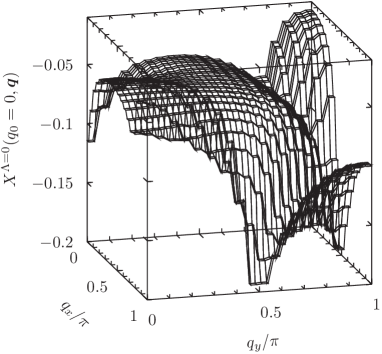
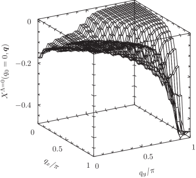
Figure 12: Momentum dependence of the static (3+1)-coupling function $X^{\Lambda=0}(0,{\bf q})$ at the end of the flow, for $t^{\prime}=-0.1$, $n=0.5$ (left) and $t^{\prime}=0$, $n=0.78$ (right). The Hubbard interaction is $U=-2$ in both cases.

We now turn to the fermion-boson vertices, whose frequency dependence is plotted in Fig. 13.

     

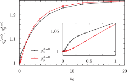
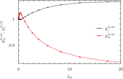
Figure 13: (Color online) Frequency dependence of the fermion-boson vertices at the end of the flow ($\Lambda=0$). Left: amplitude and phase vertices. Right: charge and magnetic vertices. The model parameters are $t^{\prime}=-0.1$, $U=-2$, and $n=0.5$.

Note that the vertices are even functions of $k_{0}$ which are normalized to one at $k_{0}=0$ by definition. The frequency dependence of the vertices is quite weak. However, the frequency dependence of the vertices in the pairing channel contributes significantly to the frequency dependence of the gap function $\Delta^{\Lambda}(k_{0})$ and also to the flow of $\Phi^{\Lambda}$. The normal self-energy and the other coupling functions are only weakly affected by the frequency dependence of the fermion-boson vertices. The magnetic vertex exhibits a small peak at low frequencies which develops at scales $\Lambda<\Lambda_{c}$ and is therefore related to pairing fluctuations.

VI.4.2 Normal self-energy and gap function

At weak to moderate interactions the ground state of the attractive Hubbard model is superfluid with Cooper pairs made of weakly renormalized quasi particles. Quasi particle renormalization occurs already at scales above the pairing scale $\Lambda_{c}$ and is described by the normal self-energy. The momentum dependence of the self-energy is weak for the choice of parameters considered in this work and we will present only results for the Fermi surface average $\Sigma^{\Lambda}(k_{0})=\langle\Sigma^{\Lambda}(k_{0},{\bf k})\rangle_{{\bf k}\in{\rm FS}}\,$. In Fig. 14 we show results for the imaginary part of $\Sigma^{\Lambda}(k_{0})$ as a function of frequency at the end of the flow ($\Lambda=0$).

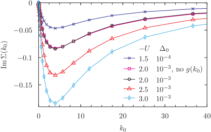
Figure 14: (Color online) Frequency dependence of the imaginary part of the normal self-energy for $t^{\prime}=-0.1$, $n=0.5$ (quarter-filling) and various choices of $U$ at the end of the flow. The result labeled as “no $g(k_{0})$” is obtained with constant (frequency-independent) fermion-boson vertices.

We plot only the positive frequency axis since ${\rm Im}\Sigma^{\Lambda}(-k_{0})=-{\rm Im}\Sigma^{\Lambda}(k_{0})$. The real part (not plotted) of $\Sigma^{\Lambda}(k_{0})$ is an even function of $k_{0}$ with a negative peak at $k_{0}=0$ that decays monotonically to the Hartree term $Un/2$ with increasing $|k_{0}|$. The overall shape of the self-energy is the same for all interaction strengths, only the size increases with $|U|$.

The slope of ${\rm Im}\Sigma^{\Lambda}(k_{0})$ at $k_{0}=0$ yields the quasi particle weight $Z_{f}^{\Lambda}$ as

$$Z_{f}^{\Lambda}=\left[1-\left.\partial_{k_{0}}{\rm Im}\Sigma^{\Lambda}(k_{0})\right|_{k_{0}=0}\right]^{-1}\,.$$ (97)

$Z_{f}=Z_{f}^{\Lambda=0}$ ranges from $Z_{f}=0.96$ for $U=-1.5$ to $Z_{f}=0.87$ for $U=-3$. Although the normal self-energy is fairly small and the quasi particle weight is only slightly suppressed for small to moderate interactions, it has nevertheless a significant impact on the size of the pairing gap.

Flows of the gap $\Delta^{\Lambda}(k_{0})$ at $k_{0}=0$ are shown in Fig. 15 for various choices of $U$.

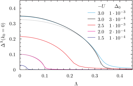
Figure 15: (Color online) Scale dependence of the gap $\Delta^{\Lambda}(k_{0})$ at $k_{0}=0$ for $t^{\prime}=-0.1$, $n=0.5$ and various choices of $U$ and $\Delta_{0}$. For $U=-2$ and $-3$, the mean-field scale-dependence $\sqrt{\Lambda_{c}^{2}-\Lambda^{2}}$, with $\Lambda_{c}$ determined from the peak of $A^{\Lambda}(0)$, is shown for comparison.

The small external pairing field $\Delta_{0}$ increases to much larger gaps at scales near and below the critical scale $\Lambda_{c}$, where $A^{\Lambda}(0)$ has a peak. The edge of the gap flow at $\Lambda_{c}$ becomes sharper for smaller $\Delta_{0}$. The gap at the end of the flow assumes values close to $\Lambda_{c}$. The scale dependence for $\Lambda<\Lambda_{c}$ obeys approximately

$$\Delta^{\Lambda}(0)\approx\sqrt{\Lambda_{c}^{2}-\Lambda^{2}}\,,$$ (98)

with increasing accuracy for smaller values of $U$ and $\Delta_{0}$. In mean-field theory this relation is exact for $\Delta_{0}\to 0$, as one can easily see by writing down the gap equation in the presence of the infrared regulator Eq. (84). For $U=-2$ the gap flow lies almost on top of the square root function Eq. (98) for small $\Delta_{0}$, while for stronger attractions deviations become visible. In particular, the final gap $\Delta^{\Lambda=0}$ becomes clearly larger than $\Lambda_{c}$.

The flow in Fig. 15 was obtained with frequency dependent effective boson propagators and fermion-boson vertices, and a frequency dependent normal self-energy and gap as described in Sec. VI.2. Comparing with results obtained by discarding the frequency dependence of some of these quantities, one finds that only the frequency dependence of the boson propagators and of the imaginary part of the normal self-energy have a substantial impact on the size of $\Delta^{\Lambda}(0)$. The feedback of the other frequency dependences on the gap at $k_{0}=0$ is small.

The critical scale and the final gap are strongly reduced compared to their mean-field values $\Lambda_{c}^{\rm MF}$ and $\Delta_{\rm MF}$, respectively, mostly due to fluctuations above the critical scale. In Fig. 16 we plot the ratio $\Delta/\Delta_{\rm MF}$ with $\Delta=\Delta^{\Lambda=0}(0)$ as a function of $U$ for $t^{\prime}=-0.1$ and $n=0.5$.

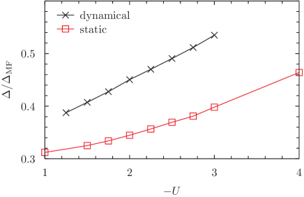
Figure 16: (Color online) Gap ratio $\Delta/\Delta_{\rm MF}$ as a function of $U$ as obtained from the flow with frequency dependent (upper curve) and static (lower curve) vertices and self-energies.

The lower curve was obtained by a simplified static parametrization of the vertex and self-energy, where all frequency dependences where neglected. Notably the reduction increases at weaker interactions and does not extrapolate to one for $U\to 0$. This is actually the expected behavior. In the weak coupling limit the gap $\Delta$ has the same exponential $U$-dependence $\Delta\propto e^{-b/|U|}$ with a (density-dependent) constant $b$ as in mean-field theory. However, the prefactor of the BCS mean-field formula is reduced by fluctuations, as first noted for the transition temperature in three-dimensional superconductors by Gorkov and Melik-Barkhudarov. gorkov61 The reduction factor in the weak coupling limit can be computed by second order perturbation theory.georges91 ; martin92 ; neumayr03 For the parameters used in Fig. 16 one finds $\Delta/\Delta_{\rm MF}\to 0.3$ for $U\to 0$.eberlein13 Both curves in Fig. 16 should tend to that value, since the flow captures the perturbative contributions. However, we cannot reach the limit $U\to 0$ numerically. It is hard to compute the gap from a numerical solution of the flow equations for smaller interaction strengths than those shown, since $\Lambda_{c}$ and $\Delta$ decrease exponentially.

For strong attractions $U$ the attractive Hubbard model can be mapped to a Heisenberg model in a uniform magnetic field. micnas90 The gap ratio $\Delta/\Delta_{\rm MF}$ thereby translates to the ratio between the staggered magnetization $m_{s}$ and the corresponding classical result $m_{s}^{\rm cl}$. From numerical results for that ratio trivedi89 one can infer that the gap ratio in the strongly attractive Hubbard model is $0.6$ at half-filling and even larger away from half-filling. The observed increase of $\Delta/\Delta_{\rm MF}$ with increasing $|U|$ is therefore consistent with the expected trend. Similar values for $\Delta/\Delta_{\rm MF}$ but with a less pronounced $U$-dependence have been obtained in an earlier fRG study with a simpler parametrization of the vertex.gersch08

We now discuss the frequency dependence of the gap function. In Fig. 17, $\Delta^{\Lambda=0}(k_{0})$ is plotted as a function of frequency for $U=-2$, $t^{\prime}=-0.1$, and $n=1/2$.

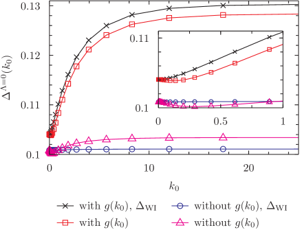
Figure 17: (Color online) Frequency dependence of the gap at the end of the flow for various approximation schemes. The inset shows the gap at small frequencies $k_{0}\leq 1$. The model parameters are $U=-2$, $t^{\prime}=-0.1$, and $n=1/2$.

Results obtained by computing the gap from a projected flow obeying the Ward identity at $k_{0}=0$ are compared to results where the frequency dependence of the gap is computed directly from the Ward identity ($\Delta_{\rm WI}$), contrasting also calculations with and without frequency dependent fermion-boson vertices $g(k_{0})$. Note that the results discussed so far were all obtained by enforcing the Ward identity only at $k_{0}=0$. Unlike the frequency dependence of the normal self-energy, the frequency dependence of the gap is strongly affected by the frequency dependent renormalization of the fermion-boson vertices. Neglecting it leads to a very weak or almost no (for $\Delta_{\rm WI}$) frequency dependence. The gap $\Delta(k_{0})$ computed by projecting the flow on the Ward identity at $k_{0}=0$ exhibits a shallow finite-frequency minimum, which is probably an artifact of the approximations associated with a (slight) violation of the Ward identity at finite frequencies. $\Delta_{\rm WI}(k_{0})$ has a minimum at $k_{0}=0$. A qualitatively similar frequency dependence of the gap is also captured by the $T$-matrix approximation.keller99

VI.4.3 Ward identity

For real gaps $\Delta_{0}$ and $\Delta^{\Lambda}$ the Ward identity, Eq. (8), can be simplified to

$$\Delta^{\Lambda}(k)-\Delta_{0}(k) = -\sum_{k^{\prime}}\Delta_{0}(k^{\prime})\,\left[G^{\Lambda}(k^{\prime})G^{\Lambda}(-k^{\prime})+\left(F^{\Lambda}(k^{\prime})\right)^{2}\right]$$ (99)

$$\times\,\left[V^{\Lambda}(k,-k,-k^{\prime},k^{\prime})-W^{\Lambda}(k,k^{\prime},k^{\prime},k)\right]\,.$$

Expressing $V^{\Lambda}$ and $W^{\Lambda}$ by the coupling functions introduced in the channel decomposition (Sec. IV), the identity can be written as

$$\Delta^{\Lambda}(k)=-\sum_{k^{\prime}}\Delta_{0}(k^{\prime})\,\left[G^{\Lambda}(k^{\prime})G^{\Lambda}(-k^{\prime})+\left(F^{\Lambda}(k^{\prime})\right)^{2}\right]\Phi_{kk^{\prime}}^{\Lambda}(0)+{\cal O}(\Delta_{0})\,,$$ (100)

for $\Delta_{0}\to 0$. The first term on the right hand side is of order one, since $\Phi_{kk^{\prime}}^{\Lambda}(0)\propto\Delta_{0}^{-1}$ for small $\Delta_{0}$. With the approximate parametrization for the Hubbard model described in Sec. VI.2, the combination of interaction terms on the right hand side of Eq. (99) can be written as

$$V^{\Lambda}(k,-k,-k^{\prime},k^{\prime})-W^{\Lambda}(k,k^{\prime},k^{\prime},k) = U+\Phi^{\Lambda}(0)g^{\Lambda}_{\phi}(k_{0})g^{\Lambda}_{\phi}(k^{\prime}_{0})$$

$$+\,\frac{1}{2}A^{\Lambda}(k^{\prime}-k)\left[g^{\Lambda}_{a}(p_{0})\right]^{2} - \frac{1}{2}\Phi^{\Lambda}(k^{\prime}-k)\left[g^{\Lambda}_{\phi}(p_{0})\right]^{2}$$

$$+\,C^{\Lambda}(k^{\prime}-k)\left[g^{\Lambda}_{c}(p_{0})\right]^{2} - 3M^{\Lambda}(k^{\prime}-k)\left[g^{\Lambda}_{m}(p_{0})\right]^{2}\,,$$ (101)

where $p_{0}=(k_{0}+k^{\prime}_{0})/2$. For a small constant $\Delta_{0}$ and a momentum-independent gap function $\Delta^{\Lambda}(k_{0})$, the Ward identity then assumes the form

$$\Delta^{\Lambda}(k_{0})=-\sum_{k^{\prime}}\Delta_{0}\left[G^{\Lambda}(k^{\prime})G^{\Lambda}(-k^{\prime})+\left(F^{\Lambda}(k^{\prime})\right)^{2}\right]\Phi^{\Lambda}(0)g^{\Lambda}_{\phi}(k_{0})g^{\Lambda}_{\phi}(k^{\prime}_{0})+{\cal O}(\Delta_{0})\,.$$ (102)

The most important consequence of the Ward identity is the divergence of the phase coupling $\Phi^{\Lambda}(0)$ in the limit $\Delta_{0}\to 0$ for $\Lambda<\Lambda_{c}$, reflecting the massless Goldstone boson associated with spontaneous symmetry breaking. The truncated flow equations do not obey the Ward identity exactly, and $\Phi^{\Lambda}(0)$ deviates from the expected behavior $\propto\Delta_{0}^{-1}$ for small $\Delta_{0}$. For small $U$ the deviations are tiny. For example, for $t^{\prime}=-0.1$, $n=1/2$, and $U=-2$, the product $\Delta_{0}\Phi^{\Lambda=0}(0)$ is almost constant down to fairly small values of $\Delta_{0}$, before it increases and finally diverges at a finite $\Delta_{0}$ of the order $10^{-5}$, which is four orders of magnitude smaller than $\Delta^{\Lambda=0}$. The same behavior was observed already in more pronounced form in Ref. gersch08, .

The violation of the Ward identity can be quantified by comparing the gap $\Delta_{\rm RG}^{\Lambda}$ computed from its flow equation to the gap $\Delta_{\rm WI}^{\Lambda}$ required by the Ward identity. The latter is computed from Eq. (99) by inserting the coupling functions as determined from the flow on the right hand side. In Fig. 18 we plot the difference $\Delta_{\rm RG}^{\Lambda}-\Delta_{\rm WI}^{\Lambda}$, divided by $\Delta_{\rm RG}^{\Lambda}U^{4}$, as a function of the scale in units of $\Lambda_{c}$.

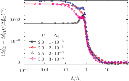
Figure 18: (Color online) Violation of the Ward identity as a function of the scale $\Lambda$ for $t^{\prime}=-0.1$, $n=1/2$ and various values of $U$ and $\Delta_{0}$. The gap $\Delta_{\rm RG}^{\Lambda}$ determined from the flow equation is compared to the gap $\Delta_{\rm WI}^{\Lambda}$ determined from the Ward identity.

One can see that the violation builds up gradually at scales around $\Lambda_{c}$. The normalized difference $(\Delta_{\rm RG}^{\Lambda}-\Delta_{\rm WI}^{\Lambda})/\Delta_{\rm RG}^{\Lambda}$ increases rapidly from $U=-2$ to $U=-3$. For $\Lambda>\Lambda_{c}$ it is roughly proportional to $U^{4}$. For $\Lambda<\Lambda_{c}$ a pronounced $\Delta_{0}$-dependence appears. For much smaller values of $\Delta_{0}$ than those shown, $\Delta_{\rm RG}^{\Lambda}-\Delta_{\rm WI}^{\Lambda}$ can turn negative, which is related to an artificial divergence of $\Phi^{\Lambda}$ at a finite $\Delta_{0}$. We observed similar $U$-dependences also for other hopping parameters and densities. On general grounds one would expect a violation of the Ward identity of order $U^{3}$ at weak coupling, even if the one-loop flow was carried out without additional approximations.katanin04 ; eberlein13 The above results suggest that the violation sets in only at order $U^{4}$, or contributions of order $U^{3}$ have very small prefactors.

In Fig. 19, $(\Delta_{\rm RG}^{\Lambda}-\Delta_{\rm WI}^{\Lambda})/\Delta_{\rm RG}^{\Lambda}$ is plotted as a function of $\Lambda$ for a fixed set of parameters, to compare the performance of different approximations.

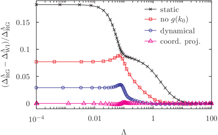
Figure 19: (Color online) Violation of the Ward identity as a function of $\Lambda$ for $U=-2$, $t^{\prime}=-0.1$, $n=1/2$, and $\Delta_{0}=10^{-3}$. Results from the flow equations with static and two distinct (with and without frequency dependent fermion-boson vertices) dynamical parametrizations of the vertex are compared to the result from the Ward identity projected flow.

The graph labeled ”dynamical” was obtained by using the frequency dependent parametrization of the vertex and the self-energy as described in Sec. VI.2. The graph ”no $g(k_{0})$” was computed with constant (unity) fermion-boson vertices, and the graph ”static” by discarding all frequency dependences. The lowest curve labeled ”coord. proj.” was computed with the dynamical parametrization and the Ward identity enforced by ”coordinate projection” (as described below). The latter obeys the Ward identity by construction, up to small discretization errors. Taking the frequency dependences into account obviously reduces the violation of the Ward identity significantly.

Even for the most accurate parametrization of the vertex, the Ward identity is not fulfilled by the truncated flow, as generally expected.katanin04 A detailed discussion of this problem in the case of superfluid order is provided in Ref. eberlein13, . The deviations are small for weak interactions but increase rapidly with $|U|$. Violating the Ward identity spoils the singular infrared behavior of the coupling functions associated with the massless Goldstone boson for $\Delta_{0}\to 0$. Even worse, it leads to artificial singularities which prevent one from carrying out the flow down to $\Lambda\to 0$ and $\Delta_{0}\to 0$. In the results presented in the preceding sections we have therefore enforced the Ward identity by using a coordinate projection procedure, devised for the numerical solution of systems of ordinary differential equations with constraints. ascher94 The flowing quantities are thereby projected on the manifold spanned by the constraint (Ward identity) in a way that the projected solution stays as close to the solution of the flow equations as possible, while deviations from the constraint are damped exponentially. In practice, we have enforced the Ward identity only at zero frequency ($k_{0}=0$), to reduce the numerical effort. eberlein13 This has little effect on absolute values of results, but leads to the slightly artificial frequency dependence of the gap at low frequencies discussed in Sec. VI.4.2.

VI.4.4 $\Delta_{0}$-flow and singularities

We finally take a closer look at the singularities of the vertex in the limit $\Delta_{0}\to 0$. In particular, we complement the numerical results for the Hubbard model by qualitative analytical estimates which are generally valid for fully gapped singlet superfluids.

To this end, we assume that the fermionic cutoff has already been removed ($\Lambda\to 0$), and we analyze the flow as a function of a decreasing pairing field $\Delta_{0}$. In Fig. 20 we show the flow of $\Delta(0)=\Delta^{\Lambda=0}(0)$, $\Phi(0)=\Phi^{\Lambda=0}(0)$ and $A(0)=A^{\Lambda=0}(0)$ as a function of $\Delta_{0}$, with an initial value $\Delta_{0}=0.005$. Results obtained for some fixed smaller values of $\Delta_{0}$ are shown for comparison.

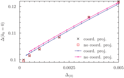
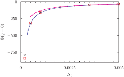
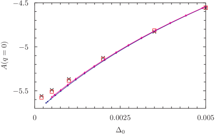
Figure 20: (Color online) $\Delta_{0}$-flows of $\Delta(0)$, $\Phi(0)$ and $A(0)$ for an initial value $\Delta_{0}=0.005$. Results obtained for fixed smaller values of $\Delta_{0}$ are shown for comparison (symbols). The model parameters are $t^{\prime}=-0.1$, $n=0.5$, $U=-2$.

The numerical computation of the $\Lambda$-flow becomes increasingly difficult at smaller $\Delta_{0}$. Furthermore, there are systematic deviations between the results obtained from the $\Delta_{0}$-flow and those computed at fixed $\Delta_{0}$. These may be related to divergencies in box diagrams for $\Delta_{0}\to 0$, which can and must be treated by a flow starting at an initially finite $\Delta_{0}$, as we discuss in the following.

In a fully gapped superfluid, the fermionic propagator is regularized by the pairing gap. However, the interaction vertex develops a singularity associated with the emergence of a Goldstone boson. In particular, the phase coupling function has the singular form

$$\Phi(q)\propto-\frac{1}{\Delta_{0}+aq_{0}^{2}+b{\bf q}^{2}}\;,$$ (103)

for small $q=(q_{0},{\bf q})$, where $a$ and $b$ are positive constants. This singularity is dictated by the Ward identity. Related singularities occur also for the imaginary parts of the pairing and anomalous (3+1)-coupling functions $P^{\prime\prime}(q)$ and $X^{\prime\prime}(q)$, respectively, but their impact is reduced by a numerator proportional to $q_{0}$. The divergence of $\Phi(q)$ for $q\to 0$, $\Delta_{0}\to 0$ is integrable in (2+1) dimensions. Hence, self-energy and vertex correction (Fig. 3) contributions involving integrals over $\Phi(q)$ remain finite for $\Delta_{0}\to 0$. However, box diagrams (Fig. 4) yield contributions involving an integral over products of two phase coupling functions,

$$\sum_{p}\partial_{\Delta_{0}}\left[G_{s_{1}s_{2}}(p-q/2)G_{s_{3}s_{4}}(p+q/2)\right]\,\Phi(p-k)\Phi(k^{\prime}-p)\,,$$ (104)

where $G$ is the propagator and $\Phi$ the phase coupling function for $\Lambda=0$. The $\Delta_{0}$-derivative of the propagators is finite for $\Delta_{0}\to 0$, but for $k=k^{\prime}$ the singularities of the phase coupling functions coalesce and the integral diverges as $\Delta_{0}^{-1/2}$. It is therefore not possible to set $\Delta_{0}$ to zero before the fermionic cutoff has been removed. The $\Delta_{0}$-flow is however well defined and integrable.

Hence, the singularities associated with the Goldstone mode do not lead to divergencies in other channels. In this respect the one-loop flow analyzed in this work is qualitatively similar to the RPA. The fluctuation effects beyond RPA yield only finite renormalizations. On the other hand, it is known from the theory of interacting bosons that the phase mode does lead to a singular renormalization of the amplitude mode.pistolesi04 In a renormalization group theory of fermionic superfluids with auxiliary boson fields representing the order parameter fluctuations, this effect appears already at one-loop level. strack08 The singular contributions involve scale derivatives acting on the boson propagators. In the purely fermionic renormalization group (without auxiliary bosons), analogous singular contributions appear only at the two-loop level.eberlein13

VII Conclusion

We have analyzed ground state properties of a spin-singlet superfluid including fluctuations on all scales via a fermionic functional renormalization group flow in a formulation that allows for symmetry breaking. The flow equations were truncated in a one-loop approximation with self-energy feedback. Spin rotation invariance and discrete symmetries were fully exploited to simplify the structure of the Nambu two-particle vertex. To parametrize the singular momentum and frequency dependences of the effective interactions, the Nambu vertex was decomposed in charge, magnetic, and various normal and anomalous pairing channels, which are all mutually coupled in the flow. We have shown that the channel decomposed one-loop flow equations are equivalent to the RPA for the vertex and to mean-field theory for the gap function, if only direct Nambu particle-hole contributions are taken into account. fn3 The crossed particle-hole and the particle-particle (in Nambu representation) contributions to the complete one-loop flow thus capture fluctuations beyond mean-field theory and RPA.

We have evaluated the flow equations for the two-dimensional attractive Hubbard model as a prototype of an interacting Fermi system with a spin-singlet superfluid ground state. The dominance of $s$-wave terms in the effective interactions in that model allows for a relatively simple parametrization. The global $U(1)$ Ward identity relating the vertex to the gap function is violated by the one-loop truncation. The deviations are very small for a weak attraction, but increase rapidly for stronger interactions. To maintain the singularity structure associated with the Goldstone boson, the flow was therefore projected on the Ward identity, analogously to evaluating a differential flow in the presence of a constraint. We have computed the effective interactions in the charge, magnetic, and pairing channels, including anomalous (3+1)-interactions describing pair annihilation (or creation) combined with a one-particle scattering process. Unprecedented comprehensive results on the momentum and (imaginary) frequency dependences of the effective interactions were obtained and discussed. The singularities in the pairing channels generated by the one-loop flow are qualitatively similar to the RPA, and are to a large extent fixed by the Ward identity. The effective magnetic interaction develops a low-frequency small-momentum peak which is a pure fluctuation effect. There are also significant quantitative fluctuation effects which are captured by the one-loop flow. In particular, the gap is strongly reduced compared to the mean-field value, with a stronger reduction at weaker interactions, as expected from perturbative and numerical results. The expected divergence of the superfluid amplitude mode in the low-energy limit is not captured by the one-loop truncation. This effect appears only at the two-loop level in the fermionic renormalization group flow.eberlein13

Besides the channel decomposition of the vertex for a system exhibiting spontaneous symmetry breaking, there are two other noteworthy technical upshots of our work, which may be picked up in future calculations. First, we have found that an accurate discretization of both momentum and frequency dependences is computationally feasible fn4 and has several advantages compared to the usual strategy of an ansatz with a small number of scale-dependent coefficients. In particular, one avoids problems with momentum or frequency derivatives which are necessary to extract the flow of such coefficients. Second, we have shown that a symmetry breaking field can be used as a convenient flow parameter, which regularizes the flow at the critical scale and allows for a controlled treatment of infrared divergences associated with the Goldstone boson.

Appendix A Pauli matrix basis

It is often convenient to represent the Nambu vertex in a basis spanned by tensor products of Pauli matrices and the unit matrix. The Pauli matrices $\tau^{(1)}$, $\tau^{(2)}$, $\tau^{(3)}$ and the unit matrix $\tau^{(0)}$ form a basis in the vector space of complex $2\times 2$ matrices. The tensor products $\tau^{(j)}\otimes\tau^{(j^{\prime})}$ form a basis in the space of complex $4\times 4$ matrices. The components of the Nambu vertex in this basis are obtained as

$$\tilde{\Gamma}^{(4)\Lambda}_{jj^{\prime}}(k_{1},k_{2},k_{3},k_{4})=\frac{1}{2}\sum_{s_{i}}\tau^{(j)}_{s_{4}s_{1}}\tau^{(j^{\prime})}_{s_{3}s_{2}}\,\Gamma^{(4)\Lambda}_{s_{1}s_{2}s_{3}s_{4}}(k_{1},k_{2},k_{3},k_{4})\;.$$ (105)

The inverse basis transformation is given by

$$\Gamma^{(4)\Lambda}_{s_{1}s_{2}s_{3}s_{4}}(k_{1},k_{2},k_{3},k_{4})=\frac{1}{2}\sum_{j,j^{\prime}}\tau^{(j)}_{s_{1}s_{4}}\tau^{(j^{\prime})}_{s_{2}s_{3}}\,\tilde{\Gamma}^{(4)\Lambda}_{jj^{\prime}}(k_{1},k_{2},k_{3},k_{4})\;.$$ (106)

The matrix formed by the components $\tilde{\Gamma}^{(4)\Lambda}_{jj^{\prime}}$ is denoted as $\tilde{\bf\Gamma}^{(4)\Lambda}$. The tilde is used to distinguish this and other matrices represented in the Pauli basis from matrices in the Nambu index basis defined in Eq. (21).

The flow equations for the coupling functions parametrizing the channel decomposed Nambu vertex can be derived most conveniently in the Pauli matrix basis. Since the complete set of coupling functions is contained in the particle-hole contribution to the vertex, their flow is determined by the flow equation Eq. (51). Transformed to the Pauli matrix basis, the equation reads

$$\frac{d}{d\Lambda}\tilde{V}^{\rm PH,\Lambda}_{jj^{\prime}}(k,k^{\prime};q)=\sum_{p}\sum_{l,l^{\prime}}\tilde{\Gamma}^{(4)\Lambda}_{jl}(k,p;q)\,\partial_{\Lambda}\tilde{L}^{\Lambda}_{ll^{\prime}}(p;q)\,\tilde{\Gamma}^{(4)\Lambda}_{l^{\prime}j^{\prime}}(p,k^{\prime};q)\;,$$ (107)

where

$$\tilde{L}^{\Lambda}_{jj^{\prime}}(p;q)=\frac{1}{2}\sum_{s_{i}}\tau^{(j)}_{s_{4}s_{1}}\tau^{(j^{\prime})}_{s_{3}s_{2}}\,G^{\Lambda}_{s_{2}s_{4}}(p-{\textstyle\frac{q}{2}})G^{\Lambda}_{s_{1}s_{3}}(p+{\textstyle\frac{q}{2}})\;.$$ (108)

The decomposition Eq. (50) of the Nambu vertex can be written in the Pauli matrix basis with momentum variables $k_{1,4}=k\pm q/2$ and $k_{2,3}=k^{\prime}\mp q/2$ as

$$\tilde{\Gamma}^{(4)\Lambda}_{jj^{\prime}}(k,k^{\prime};q) = \tilde{U}_{jj^{\prime}}(k,k^{\prime};q)+\tilde{V}^{\rm PH,\Lambda}_{jj^{\prime}}(k,k^{\prime};q)$$ (109)

$$- \tilde{V}^{\rm PH^{\prime},\Lambda}_{jj^{\prime}}\left(\textstyle{\frac{k+k^{\prime}-q}{2},\frac{k+k^{\prime}+q}{2};k^{\prime}-k}\right)$$

$$+ \tilde{V}^{\rm PP,\Lambda}_{jj^{\prime}}\left(\textstyle{\frac{k-k^{\prime}+q}{2},\frac{k-k^{\prime}-q}{2};k+k^{\prime}}\right)\;.$$

Note that $\tilde{V}^{\rm PH^{\prime},\Lambda}_{jj^{\prime}}$ is defined by transforming $V^{\rm PH,\Lambda}_{s_{2}s_{1}s_{3}s_{4}}$ with the first two Nambu indices exchanged to the Pauli matrix basis. The functions $\tilde{L}^{\Lambda}_{jj^{\prime}}(p;q)$ are given by products of normal and anomalous propagators,

$$L^{\Lambda}_{00}(p;q) = {\rm Re}[G^{\Lambda}(p_{-})G^{\Lambda}(p_{+})]+F^{\Lambda}(p_{-})F^{\Lambda}(p_{+})\;,$$

$$L^{\Lambda}_{01}(p;q) = iF^{\Lambda}(p_{-}){\rm Im}G^{\Lambda}(p_{+})+i{\rm Im}G^{\Lambda}(p_{-})F^{\Lambda}(p_{+})=L^{\Lambda}_{10}(p;q)\;,$$

$$L^{\Lambda}_{02}(p;q) = i{\rm Re}G^{\Lambda}(p_{-})F^{\Lambda}(p_{+})-iF^{\Lambda}(p_{-}){\rm Re}G^{\Lambda}(p_{+})=-L^{\Lambda}_{20}(p;q)\;,$$

$$L^{\Lambda}_{03}(p;q) = i{\rm Im}[G^{\Lambda}(p_{-})G^{\Lambda}(p_{+})]=L^{\Lambda}_{30}(p;q)\;,$$

$$L^{\Lambda}_{11}(p;q) = -{\rm Re}[G^{\Lambda}(p_{-})G^{\Lambda*}(p_{+})]+F^{\Lambda}(p_{-})F^{\Lambda}(p_{+})\;,$$

$$L^{\Lambda}_{22}(p;q) = -{\rm Re}[G^{\Lambda}(p_{-})G^{\Lambda*}(p_{+})]-F^{\Lambda}(p_{-})F^{\Lambda}(p_{+})\;,$$

$$L^{\Lambda}_{33}(p;q) = {\rm Re}[G^{\Lambda}(p_{-})G^{\Lambda}(p_{+})]-F^{\Lambda}(p_{-})F^{\Lambda}(p_{+})\;,$$

$$L^{\Lambda}_{12}(p;q) = {\rm Im}[G^{\Lambda}(p_{-})G^{\Lambda*}(p_{+})]=-L^{\Lambda}_{21}(p;q)\;,$$

$$L^{\Lambda}_{13}(p;q) = {\rm Re}G^{\Lambda}(p_{-})F^{\Lambda}(p_{+})+F^{\Lambda}(p_{-}){\rm Re}G^{\Lambda}(p_{+})=L^{\Lambda}_{31}(p;q)\;,$$

$$L^{\Lambda}_{23}(p;q) = {\rm Im}G^{\Lambda}(p_{-})F^{\Lambda}(p_{+})-F^{\Lambda}(p_{-}){\rm Im}G^{\Lambda}(p_{+})=-L^{\Lambda}_{32}(p;q)\;,$$ (110)

where $p_{+}=p+q/2$, $p_{-}=p-q/2$.

The matrices representing the Nambu vertex in our approximation for the Hubbard model are not all full, that is, several matrix elements vanish. More generally, for coupling functions with a factorized momentum dependence and even parity form factors the (direct) particle-hole contribution to the vertex has the form

$$\tilde{\bf V}^{\rm PH,\Lambda}(k,k^{\prime};q)=\left(\begin{array}[]{cccc}2M^{\Lambda}_{kk^{\prime}}(q)&0&0&0\\ 0&A^{\Lambda}_{kk^{\prime}}(q)&P^{\prime\prime\Lambda}_{kk^{\prime}}(q)&2X^{\prime\Lambda}_{kk^{\prime}}(q)\\ 0&-P^{\prime\prime\Lambda}_{kk^{\prime}}(q)&\Phi^{\Lambda}_{kk^{\prime}}(q)&-2X^{\prime\prime\Lambda}_{kk^{\prime}}(q)\\ 0&2X^{\prime\Lambda}_{kk^{\prime}}(q)&2X^{\prime\prime\Lambda}_{kk^{\prime}}(q)&2C^{\Lambda}_{kk^{\prime}}(q)\end{array}\right)\;,$$ (111)

and the particle-particle contribution $\tilde{\bf V}^{\rm PP,\Lambda}$ has only diagonal elements given by the magnetic coupling function $M^{\Lambda}_{kk^{\prime}}(q)$. However, the matrix elements of the crossed particle-hole contribution $\tilde{\bf V}^{\rm PH^{\prime},\Lambda}(k,k^{\prime};q)$ are all non-zero and generally given by linear combinations of several coupling functions.

References

- (1) D. M. Eagles, Phys. Rev. 186, 456 (1969).
- (2) A. J. Leggett, in Modern Trends of Condensed Matter, edited by A. Pekalski and J. Przystawa (Springer, Berlin, 1980).
- (3) W. Zwerger (Ed.), The BCS-BEC Crossover and the Unitary Fermi Gas (Springer, Berlin, 2012).
- (4) W. Metzner, M. Salmhofer, C. Honerkamp, V. Meden, and K. Schönhammer, Rev. Mod. Phys. 84, 299 (2012).
- (5) C. Wetterich, Phys. Lett. B 301, 90 (1993).
- (6) J. Berges, N. Tetradis, and C. Wetterich, Phys. Rep. 363, 223 (2002).
- (7) P. Kopietz, L. Bartosch, and F. Schütz, Introduction to the Functional Renormalization Group (Springer, Berlin, 2010).
- (8) D. Zanchi and H. J. Schulz, Phys. Rev. B 61, 13609 (2000).
- (9) C. J. Halboth and W. Metzner, Phys. Rev. B 61, 7364 (2000).
- (10) C. Honerkamp, M. Salmhofer, N. Furukawa, and T. M. Rice, Phys. Rev. B 63, 035109 (2001).
- (11) T. Baier, E. Bick, and C. Wetterich, Phys. Rev. B 70, 125111 (2004).
- (12) H. C. Krahl, S. Friederich, and C. Wetterich, Phys. Rev. B 80, 014436 (2009).
- (13) M. C. Birse, B. Krippa, J. A. McGovern, and N. R. Walet, Phys. Lett. B 605, 287 (2005).
- (14) S. Diehl, H. Gies, J. M. Pawlowski, and C. Wetterich, Phys. Rev. A 76, 021602(R) (2007).
- (15) B. Krippa, Eur. Phys. J. A 31, 734 (2007).
- (16) P. Strack, R. Gersch, and W. Metzner, Phys. Rev. B 78, 014522 (2008).
- (17) S. Floerchinger, M. Scherer, S. Diehl, and C. Wetterich, Phys. Rev. B 78, 174528 (2008).
- (18) L. Bartosch, P. Kopietz, and A. Ferraz, Phys. Rev. B 80, 104514 (2009).
- (19) H. C. Krahl, J. A. Müller, and C. Wetterich, Phys. Rev. B 79, 094526 (2009).
- (20) S. Friederich, H. C. Krahl, and C. Wetterich, Phys. Rev. B 81, 235108 (2010); ibid. 83, 155125 (2011).
- (21) M. Salmhofer, C. Honerkamp, W. Metzner, and O. Lauscher, Prog. Theor. Phys. 112, 943 (2004).
- (22) R. Gersch, C. Honerkamp, D. Rohe, and W. Metzner, Eur. Phys. J. B 48, 349 (2005).
- (23) R. Gersch, C. Honerkamp, and W. Metzner, New J. Phys. 10, 045003 (2008).
- (24) A. Eberlein and W. Metzner, Prog. Theor. Phys. 124, 471 (2010); note that fermionic propagators are defined with a different sign convention in that work.
- (25) C. Husemann and M. Salmhofer, Phys. Rev. B 79, 195125 (2009).
- (26) A similar channel decomposition was derived and applied also for the single-impurity Anderson model by C. Karrasch, R. Hedden, R. Peters, T. Pruschke, K. Schönhammer, and V. Meden, J. Phys. Condens. Matter 20, 345205 (2008).
- (27) A. A. Katanin, Phys. Rev. B 70, 115109 (2004).
- (28) M. Salmhofer and C. Honerkamp, Prog. Theor. Phys. 105, 1 (2001).
- (29) In the matrix presented in Ref. eberlein10, , Eq. (3.18), the order of the first two momenta of the matrix elements and was erroneously reversed.
- (30) S. A. Maier and C. Honerkamp, Phys. Rev. B 86, 134404 (2012).
- (31) For a review of the attractive Hubbard model, see R. Micnas, J. Ranninger, and S. Robaszkiewicz, Rev. Mod. Phys. 62, 113 (1990).
- (32) R. Frèsard, B. Glaser, and P. Wölfle, J. Phys.: Condens. Matter 4, 8565 (1992).
- (33) M. H. Pedersen, J. J. Rodríguez-Núnez, H. Beck, T. Schneider, and S. Schafroth, Z. Phys. B 103, 21 (1997).
- (34) M. Letz and R. J. Gooding, J. Phys.: Condens. Matter 10, 6931 (1998).
- (35) M. Keller, W. Metzner, and U. Schollwöck, Phys. Rev. B 60, 3499 (1999).
- (36) M. Randeria, N. Trivedi, A. Moreo, and R. T. Scalettar, Phys. Rev. Lett. 69, 2001 (1992); N. Trivedi and M. Randeria, ibid. 75, 312 (1995).
- (37) R. R. dos Santos, Phys. Rev. B 50, 635 (1994).
- (38) J. M. Singer, M. H. Pedersen, T. Schneider, H. Beck, and H.-G. Matuttis, Phys. Rev. B 54, 1286 (1996).
- (39) M. Keller, W. Metzner, and U. Schollwöck, Phys. Rev. Lett. 86, 4612 (2001); J. Low Temp. Phys. 126, 961 (2002).
- (40) M. Capone, C. Castellani, and M. Grilli, Phys. Rev. Lett. 88, 126403 (2002).
- (41) A. Neumayr and W. Metzner, Phys. Rev. B 67, 035112 (2003).
- (42) R. Shankar, Rev. Mod. Phys. 66, 129 (1994).
- (43) C. Husemann, K.-U. Giering, and M. Salmhofer, Phys. Rev. B 85, 075121 (2012).
- (44) A. Eberlein, PhD thesis, University Stuttgart (2013).
- (45) See, for example, T. Holder and W. Metzner, Phys. Rev. B 85, 165130 (2012).
- (46) K.-U. Giering and M. Salmhofer, Phys. Rev. B 86, 245122 (2012).
- (47) L. P. Gorkov and T. K. Melik-Barkhudarov, Sov. Phys. JETP 13 1018 (1961).
- (48) A. Georges and J. S. Yedidia, Phys. Rev. B 43, 3475 (1991).
- (49) A. Martin-Rodero and F. Flores, Phys. Rev. B 45, 13008 (1992).
- (50) See, for example, N. Trivedi and D. M. Ceperley, Phys. Rev. B 40, 2737 (1989); A. Lüscher and A. M. Läuchli, Phys. Rev. B 79, 195102 (2009).
- (51) U. M. Ascher, H. Chin, and S. Reich, Numer. Math. 67, 131 (1994).
- (52) See, for example, F. Pistolesi, C. Castellani, C. Di Castro, and G. C. Strinati, Phys. Rev. B 69, 024513 (2004), and references therein.
- (53) Recall that the Cooper (particle-particle) contributions are transformed to particle-hole terms in Nambu representation.
- (54) For flows in the symmetric regime a treatment of momentum and frequency dependences by discretization has been used already by Giering and Salmhofer, see Ref. giering12, .