Bayesian Model Averaging in Astrophysics: A Review

Abstract

We review the use of Bayesian Model Averaging in astrophysics. We first introduce the statistical basis of Bayesian Model Selection and Model Averaging. We discuss methods to calculate the model-averaged posteriors, including Markov Chain Monte Carlo (MCMC), nested sampling, Population Monte Carlo, and Reversible Jump MCMC. We then review some applications of Bayesian Model Averaging in astrophysics, including measurements of the dark energy and primordial power spectrum parameters in cosmology, cluster weak lensing and Sunyaev–Zel’dovich effect data, estimating distances to Cepheids, and classifying variable stars.

Keywords

cosmology: methods: data analysis – methods: statistical

1 Introduction

We are in an unparalleled time in modern astrophysics, a belle epoque where more datasets and theoretical models are available than ever before, with the number increasing at an exponential rate. This is driven by Moore’s law, as new technology has allowed the development of better detectors to make observations and more powerful computers to produce simulations.

In the middle, acting as the interface between these two areas, is the field of statistical analysis, and again the growth in available processing power has had a remarkable impact. Before the last decade, Bayesian statistics were rarely applied in astrophysics, due to the computationally intensive nature of computing the relevant quantities accurately. Now posterior samples and model selection statistics can be computed fast enough that the space of possible theories can be fully investigated. Comprehensive overviews of Bayesian methodology are given by MacKay, Gregory, and Sivia & Skilling [1, 2, 3]; for a collection of articles on such methods as applied to cosmology see ref [4].

The strength of Bayesian methods is the ability to assign a probability value to a model directly, based on the parameter ranges allowed and the data available. Model selection should proceed first, before parameter estimation, and only once the best model has been found should the parameters be estimated. Often though, the data is not strong enough to distinguish decisively between the models. In this case, computing the parameter constraints under the assumption of an individual model underestimate the true uncertainty of those parameters.

The solution to this problem is Bayesian Model Averaging, where the uncertainty as to the correct model is folded into the calculation of the parameter probabilities. Each individual posterior, generated under the assumption of a particular model, is weighted by the model likelihood and then combined with the others to give the model-independent posterior. In this paper we review Bayesian Model Averaging and its previous applications in astrophysics and cosmology.

In our review we found that Bayesian Model Averaging is used in two manners. Firstly there are those situtations where the likelihood is well understood and it is only the nature of the prior models and parameters that are varied and averaged over. This is typically the case in cosmology, where the cosmic microwave background (CMB) and distance rulers are well measured observables. However, these observations indicate the existence of new physical processes, such as inflation and dark energy, for which there are no well-established physical mechanisms. Then there are the cases where the physical model being investigated is well understood, but the model of data acquisition or interpretation is more ambiguous, leading to nuisance models that need to be averaged over. This is the case for galaxy clusters, Cepheid variable distances, and star classification. Of course this kind of division can be somewhat arbitrary, as the models considered as nuisance for one investigator maybe of great interest for another.

In Section 2 we introduce the ideas of Bayesian Model Selection and Model Averaging. In Section 3 we discuss some of the methods used to compute the model-averaged posterior distributions, while in Section 4 we review the applications of Bayesian Model Averaging that exists in the astrophysics literature. In Section 5 we conclude.

2 Model selection and model averaging

Bayes’ theorem states the relationship between models ($\mathcal{M}$), parameters ($\bar{\theta}$), and data ($D$)

$$P(\bar{\theta}|D,\mathcal{M})=\frac{P(D|\bar{\theta},\mathcal{M})P(\bar{\theta}|\mathcal{M})}{P(D|\mathcal{M})}\,,$$ (1)

where $P(\bar{\theta}|\mathcal{M})$ is the prior probability distribution of the parameters (assuming some model $\mathcal{M}$), $P(D|\bar{\theta},\mathcal{M})$ is the likelihood, and $P(\bar{\theta}|D,\mathcal{M})$ is the posterior probability distribution of the parameters. The prior is updated to the posterior by the likelihood. The term $P(D|\mathcal{M})$ represents the model likelihood, and is called the evidence. In the case of single-model inference (where only a single model or set of parameters is considered), the evidence is simply a normalizing constant, set to satisfy the condition that the posterior distribution sums to unity.

However, in most interesting cases in astrophysics, the correct model is not known, and the evidence takes different values for different models. We can use Bayes’ theorem again, at one level above, to calculate the posterior odds between different models and perform model selection,

$$\frac{P(\mathcal{M}_{1}|D)}{P(\mathcal{M}_{2}|D)}=\frac{P(D|\mathcal{M}_{1})}{P(D|\mathcal{M}_{2})}\frac{P(\mathcal{M}_{1})}{P(\mathcal{M}_{2})}\,.$$ (2)

Here $\mathcal{M}_{1}$ and $\mathcal{M}_{2}$ are the different models under consideration, $P(\mathcal{M}_{i})$ gives the prior probability of each model, and $P(\mathcal{M}_{i}|D)$ is the model posterior probability. Thus the model posterior probability is updated from the prior by the evidence. If the model priors are equal then the ratio of posteriors is simply the ratio of evidences. The ratio of evidences is commonly known as the Bayes factor $B$ [5], and an interpretation scale was suggested by [6] (though some authors have started to use different language to qualify the different levels, e.g. [7]). Many papers have already been written about the use of the evidence for cosmological model selection, a collection of the earliest being [8, 9, 10, 11, 12, 13, 14, 15]. For reviews see refs [16, 17, 18].

The logical procedure would be to first perform a model selection analysis to find the best model. Having done so, we would then perform parameter inference for the parameters of that single best model. However it is possible, even likely, that no model will have decisive evidence ($\ln B>5$) over all competing models. If we want to include this model uncertainty in the parameter posteriors, we can instead produce a model-averaged posterior distribution [19], where the individual posteriors from each model are summed together, weighted by the model posterior values:

$$P(\bar{\theta}|D)=\frac{\sum_{k}P(\bar{\theta}|D,\mathcal{M}_{k})P(\mathcal{M}_{k}|D)}{\sum_{k}P(\mathcal{M}_{k}|D)}\,.$$ (3)

This model-averaged posterior encodes the uncertainty as to the correct model.

3 Methods

Bayesian Model Averaging requires the computation of two quantities per model, the individual model posterior and the evidence. Astrophysical data are complex, requiring (at the very least) differential equations to be integrated over time and/or space to make predictions that can be tested against observations. As such, almost no likelihood function can be solved for analytically, and so the posterior and evidence have to be estimated by sampling methods.

Since such Bayesian methods, especially model selection and model averaging, have only recently become popular in their application in astrophysics, there are quite a number of methods available in the statistics literature that remain unconsidered in this review. For overview of some other methods see, for example ref [20].

3.1 Markov Chain Monte Carlo

Markov Chain Monte Carlo is a sampling method whose objective is to generate a chain of sampled parameter values that obeys Markovian statistics, and has the distribution being sampled as its equilibrium distribution. Estimates of the underlying moments of the probability distribution are simply estimates of the moments of the chain, for example the mean $\mu$ and variance $\sigma^{2}$ given by

$$\mu=E(\theta) = \frac{1}{n}\sum_{i=1}^{n}\theta_{i}\,,$$ (4)

$$\sigma^{2}=E((\theta-\mu)^{2}) = \frac{1}{n}\sum_{i=1}^{n}(\theta_{i}-\mu)^{2}\,.$$ (5)

Similarly, we could use the chain to estimate the evidence,

$$P(D|M)=E\simeq\frac{1}{n}\sum_{i=1}^{n}L(\theta_{i}){\rm Pr}(\theta_{i})\,,$$ (6)

where $L(\theta)$ is the likelihood, $P(D|\theta,M)$, and ${\rm Pr}(\theta)$ is the prior, $P(\theta|D)$, but this does not provide a valid (either unbiased or converging) approximation.

Since samples cannot be drawn directly from the distribution initially, MCMC conducts a random walk through the available parameter space, generating points and adding them to the chain based on a set of rules. The most common form of MCMC used in astrophysics is the Metropolis–Hastings algorithm [21, 22].

MCMC has been used to generate posterior samples for a wide variety of problems in astrophysics, becoming prevalent in cosmology following the creation of the CosmoMC code by Lewis and Bridle [23]. MCMC methods are very efficient at tracing uni-modal posterior probability distributions without pronounced degeneracies in the vicinity of the best-fit region. However, the evidence calculation receives non-negligible contributions from the tails of the distribution, because even though the likelihoods there are small, this region occupies a large volume of the prior probability space. To compute the evidence accurately, the entire prior space has to be sampled, which can take a very long time using simple MCMC methods.

3.2 Nested sampling

The nested sampling algorithm was devised by Skilling [24, 25] as a method to compute the evidence. Nested sampling is a Monte Carlo method that recasts the multi-dimensional evidence integral as a one-dimensional integral in terms of the prior mass X, where $dX={\rm Pr}(\theta)d\theta$, with $X$ running from 0 to 1. The integral is simply the sum of the likelihood-weighted prior mass samples,

$$E=\int L(X)dX=\sum_{j=1}^{m}E_{j}~{},~{}~{}E_{j}=\frac{L_{j}}{2}(X_{j-1}+X_{j+1})\,.$$ (7)

This is shown in Figure 1.

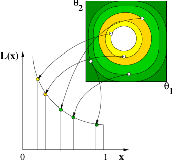
Figure 1: A schematic of the nested sampling algorithm. The two-dimensional parameter space is shown at the top right. The points within it are considered to represent contours of constant likelihood, which sit within each other like layers of an onion (there is however no need for them to be simply connected). The volume corresponding to each thin shell of likelihood is computed by the algorithm, allowing the integral for the evidence to be accumulated as shown in the graph. (From [26])

In order to compute the integral accurately the prior mass is logarithmically sampled. Firstly a set of $N$ ‘live’ points is randomly distributed within the prior parameter space. Then the lowest likelihood point $L_{j}$ is discarded, replaced by a new point uniformly sampled from the remaining prior mass (i.e. it must have a likelihood greater than $L_{j}$). At every iteration the remaining prior mass, $X_{j}$, shrinks by a known probabilistic factor that can be estimated from the number of live points, and the evidence is incremented accordingly. In this way the algorithm works its way towards the higher likelihood regions.

Nested sampling was adapted for use in cosmology by Mukherjee, et al. [26], creating the CosmoNest code, and by [27], with MultiNest. The key challenge of applying nested sampling is the uniform sampling of the remaining prior mass (as if the sampling is not uniform, the resulting Evidence value will be biased). CosmoNest achieved this by creating a single ellipsoid with contained all the remaining live points, and sampling uniformly from this shape. MultiNest advanced this to automatically generate multiple ellipsoids, to cover multiple likelihood peaks and increase the efficiency of the sampling process.

One of the advantages of using nested sampling is that the samples, as well as contributing to the evidence integral, can also be used as posterior samples. Although they don’t obey Markovian statistics, their posterior weight can easily be calculated from Bayes’ theorem, using their likelihood and the prior mass associated with them.

3.3 Population Monte Carlo

Population Monte Carlo is a generic adaptive importance sampling method [28]. Importance sampling is the idea that you can generate your samples completely stochastically from some distribution. In importance sampling we draw samples from some proposal distribution $q$, such that more samples are drawn from regions which are judged to be important. The weights of each of the samples is given as

$$w_{i}=\frac{P(X_{i})}{q(X_{i})}\,;~{}~{}~{}~{}i=1,\ldots,N$$ (8)

For example, if there is some new data that will update constraints already in place from some previous experiment, you could simply recompute the new posterior ($P$) at points given by a previous MCMC chain (the values of $q$), importance sampling using the chain as the proposal distribution. Obviously the distribution of points is unchanged, but the new likelihoods give the new weights (or importances) of the samples.

Similarly to MCMC, we can use importance sampling to compute the evidence, since it will simply be the average of the weights,

$$E\approx\frac{1}{N}\sum_{i=1}^{N}w_{i}\,.$$ (9)

Adaptive Importance Sampling (otherwise known as Population Monte Carlo) updates the proposal distribution with each iteration, attempting to move it closer to the distribution being sampled. Douc et al [29] proposed to minimize the distance between the target distribution $\pi$ (our posterior) and the proposal distribution $q$ as defined by the Kullback–Leibler divergence (the relative Shannon entropy between the two distributions [30]). This is defined to be

$$D_{\rm KL}(p||q)=\int p(\theta)\log\frac{p(\theta)}{q(\theta)}d\theta\,,$$ (10)

where $p$ and $q$ are two distributions, and $x$ is a set of variables that the distributions depend on. Rather than integrate over the parameter space, we can compute this function by simply summing it over the samples, i.e.

$$D_{\rm KL}(\pi||q)\approx\sum_{i=1}^{N}P(\theta_{i})\log\frac{P(\theta_{i})}{q(\theta_{i})}\,.$$ (11)

Kilbinger et al. [31], following the approach of Cappé et al. [28, 32], applied Population Monte-Carlo to cosmology, using an implementation where the importance function $q$ were modelled by a sum of mixtures

$$q_{X}(x)=\sum_{d=1}^{D}\alpha_{d}f_{Y_{d}}(x)\,.$$ (12)

where $\alpha=(\alpha_{1},\dots,\alpha_{D})$ is a vector of adaptable weights for the mixture components (with $\alpha_{d}>0$ and $\sum_{d=1}^{D}\alpha_{d}=1$) and $Y_{d}$ a vector that specifies the components. Here $f$ is a parameterized probability density function, usually taken to be a multi-variate Gaussian or Student-t distribution. In these cases, the updated weights and distribution parameters that minimise the KL divergence between the two distributions can be solved for analytically, details of which can be found in ref. [32].

Table 1: List of cosmological parameters and their approximate date of introduction into the standard cosmological model.

Cosmological parameter	Symbol	Introduction date	Alternate versions
Hubble parameter	$H_{0}$	1929	Distance to last scattering surface $\Theta$
Matter density	$\Omega_{\rm m}$	1924	Physical matter density, $\omega_{\rm m}=\Omega_{\rm m}h^{2}$
CMB Temperature	$T_{\rm CMB}$	1964	Radiation density $\Omega_{\rm r}$
Cold Dark Matter density	$\Omega_{\rm c}$	(1933) 1975
Galaxy Bias	$b$	1985
Amplitude of density perturbations	$A_{\rm s}$	1992	CMB normalization $\Delta T/T$, dispersion at $8h^{-1}$Mpc, $\sigma_{8}$
Optical depth to reionization	$\tau$	2003	Redshift of reionization, $z_{\rm reion}$
Spectral index of scalar perturbations	$n_{\rm s}$	2006

Population Monte Carlo suffers from some of the problems faced by ordinary MCMC. For example, when the mixture distribution doesn’t cover all the modes in a multi-modal distribution, it will fail to pick up contributions from these modes.

One advantage of PMC is that it allows us to break somewhat from the ‘sequential tyranny’ of ordinary Markov Chain methods. Since the importance function is known, large numbers of samples can be generated from it in parallel, making it ideally suited for use in Graphics Processing Unit (GPU) computing, since the GPUs can perform a very large number of parallel floating point operations. Of course, the update step still requires these samples to be brought together and analysed so that the importance function can be updated. Kilbinger et al. [31] state that PMC gives an unbiased estimator of the evidence at each iteration, and will converge on a high accuracy value in a very small number of such iterations.

As with Nested Sampling, PMC produces samples of the posterior, and so can be used for generating model averaged posteriors.

3.4 Transdimensional MCMC

The biggest time requirement in using these previous methods for Bayesian Model Averaging is that the posteriors and evidences for each model need to be computed for each model individually. It could be more efficient to instead do all of this in one step, simultaneously sampling from the model space as well as the parameter values. For this we need an MCMC algorithm that can change dimensionality, while still maintaining reversibility to guarantee the chains elements satisfy detailed balance. Examples of transdimensional Monte Carlo include Reversible Jump MCMC [33] birth-and-death process Monte-Carlo [34], and Continuous Time MCMC [35].

Reversible Jump MCMC is an algorithm in which the dimensionality of the model can be changed during the chain, by allowing transitions between models as well as parameter values. In order to maintain detailed balance, Green (1995) proposed a new acceptance probability. The general acceptance ratio from state $X=(1,\theta^{(1)})$ to state $X=(2,\theta^{(2)})$, where 1 and 2 represent the model spaces that the two different states occupy, as

$$\alpha_{m}(X,X^{\prime}) =$$

$${\rm min}\left\{1,\frac{P(2,\theta^{(2)}|D)j(2,\theta^{(2)})q_{2}(u^{(2)})}{P(1,\theta^{(1)}|D)j(1,\theta^{(1)})q_{1}(u^{(1)})}\left\|\frac{\partial g(\theta^{(2)},u^{(2)})}{\partial(\theta^{(1)},u^{(1)})}\right\|\right\}\,,$$

where $P(\theta|D)$ is the usual posterior value, $q$ is the probability density for parameter values inside that model, $j$ is the probability for steps between models, and $u$ is an extra random variable that controls the proposal of different models. The final term is a Jacobian of the function $g(\theta,u)$ that converts parameter values between models, i.e. $(\theta^{(1)},u^{(1)})=g(\theta^{(2)},u^{(2)})$. If these are independent, then the Jacobian is simply unity.

The drawback of RJMCMC is that in practice, for the case of a small number of models, it isn’t more efficient to sample simultaneously in both model and parameter space, since the steps between models often have a low acceptance rate. Instead, RJMCMC is more useful in cases where the dimensionality of the problem is large. For example, it has been applied in astrophysics to detection problems where the number of sources is unknown, such as in gravitational wave astronomy [36].

4 Applications in Astrophysics

4.1 Cosmological Parameters

Cosmological model development has proceeded incrementally, with a new parameter being added to the concordance cosmological model at a rate of approximately one a decade (though starting to increase faster in recent years: see Table 1 for an approximate history). Cosmological models rarely make specific predictions for the values of the parameters. For example, there is no theory that predicts exactly the value of the Hubble parameter, though you can infer a plausible range from other data, such as the age of the oldest stars in the Universe. The models that do predict values for the observables, for example models of inflation that predict specific values of $n_{\rm s}$ (the spectral index) and $r$ (the tensor-to-scalar amplitude ratio), do so by changing the free parameter to something more fundamental to the theory (e.g. the value of the mass scale or coupling in the inflationary potential).

Therefore, because there are no fundamental models that make very accurate predictions for the values of the cosmological parameters, they are phenomenological parameters. They can be measured accurately, but little or no fundamental physics can (yet) be derived from them. This isn’t true for all cosmological parameters, and may not be always true for others. The optical depth to reionization, for example, could be accurately predicted if we had a perfect model for the formation of the first generation of stars and the reionization of the cosmic hydrogen. Alas, perfect models are found only in mathematics, and physicists have to live in the real Universe.

The lack of a good theory to predict these parameters means that the relevant priors may be subject to a level of contention.

4.1.1 Dark Energy

The mysterious dark energy makes up around 70% of the energy density of the Universe, and acts against gravity to drive an accelerating expansion. Its discovery in the late 1990s was largely unexpected, and even today there are no very compelling models for where it comes from. The Dark Energy Task force report stated that “the nature of dark energy ranks among the very most compelling of all outstanding problems in physical science.” [37].

The dynamical properties of the dark energy are normally parameterized in terms of the equation of state parameter $w$, where

$$w=\frac{P}{\rho}\,.$$ (14)

Here $P$ is the pressure of the dark energy fluid and $\rho$ is the density. Different models of the dark energy make different predictions for the value of the equation of state. The cosmological constant model, where the dark energy is the zero-point energy of the vacuum, predicts a value of $w=-1$ only. Quintessence models, where canonical scalar fields are slowly rolling down some potential, can take time-dependent values in the range $-1<w<1$.

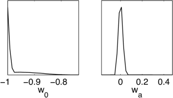
Figure 2: Posterior parameter distributions for dark energy equation of state parameters $w_{0}$ (the value today) and $w_{a}$ (the rate of change with scale factor). These distributions were obtained using the WMAP+SDSS(BAO)+SNLS data combination averaging over the quintessence-type models (I, II and V) alone. Some smoothing of the delta-functions has been carried out by binning. (From [38])

Liddle et al. [38] addressed the problem of model independent constraints on the equation of state parameter $w$ where the correct model is not known. They used five different models for the equation of state, which were:

1. The cosmological constant model, where $w=-1$ at all times,

2. A constant equation of state model, where $w$ can vary in the range $-1<w<-1/3$,

3. A constant equation of state model, where $w$ can vary in the wider range $-2<w<-1/3$,

4. A time-varying equation of state, where the two parameters have prior range $-2<w_{0}<-1/3$ and $-4/3<w_{a}<4/3$,

5. A time varying equation of state, where the equation of state as a function of scale factor has prior range $-1<w(a)<1$.

Models (ii) and (v) placed priors on the equation of state that excluded some of the high-likelihood region found in models (iii) and (iv), but these models were created to enforce the weak energy condition. In models (iv) and (v) the CPL parameterization [39, 40] was used, where

$$w(a)=w_{0}+(1-a)w_{a}\,.$$ (15)

They also varied two parameters common between all five models, the present fractional energy density of matter $\Omega_{\rm m}$ and the value of the Hubble parameter today $H_{0}$. They assumed a flat universe where the density of the dark energy $\Omega_{\rm DE}=1-\Omega_{\rm m}$.

In terms of data used to compute the evidence of each of the models and the posteriors of the parameters, they used distance data from the then-current three-year Wilkinson Microwave Anisotropy Probe (WMAP) observations [41, 42], the BAO measurement from the Sloan Digital Sky Survey (SDSS) LRG sample [43], and SN Ia data from the HST/GOODS programme [44] and the first-year Supernova Legacy Survey (SNLS [45]), together with nearby SN Ia data. They computed the evidence and the posteriors simultaneously using nested sampling.

The model selection results were inconclusive with no model favoured and only model (v) significantly disfavoured. Of course, owing to the nature of the different priors allowing different high likelihood regions, the posteriors for the five models were very different. The authors used Bayesian Model Averaging to plot the model-averaged posterior for $w_{0}$ and $w_{a}$, averaging over all five models and also those that enforced the weak energy condition (i, ii and v). The results are shown in Figure 2.

4.1.2 Curvature

In [46], the authors conducted a similar analysis to Liddle et al. [38], which was described in section 4.1.1, using more up-to-date data and including models for the curvature of the universe simultaneously. They utilized data from the WMAP five-year release [47], once again using only the distance data from the CMB, the updated BAO measurements from [48], and the UNION08 SN-Ia data compilation [49]. They considered only three different models for the dark energy, which were:

$\Lambda$: The cosmological constant model, where $w=-1$ at all times,

W: A constant equation of state model, where $w$ can vary in the range $-2<w<-1/3$, and $w_{a}=0$,

WZ: A time-varying equation of state, where the two parameters have prior range $-2<w_{0}<-1/3$ and $-4/3<w_{a}<4/3$.

They also considered three models of the curvature of the universe: flat, open, and closed. However, interestingly they considered these three models with two different priors, effectively measuring two different parameters. The Astronomers’ prior considered $\Omega_{k}$ as the parameter to be measured. The Curvature scale prior considered the curvature scale (the log of $\Omega_{k}$ or $-\Omega_{k}$ depending on whether the model was open or closed) as the parameter to be varied. They combined the three dark energy models and the three curvature models together (creating nine different models in total) for each of the two choices of prior.

They used Metropolis–Hastings Markov Chain Monte Carlo to compute the posterior distributions and Bayes factors. They found that no model was favoured over the flat $\Lambda$ model, but the closed or open models with the Astronomers’ prior were significantly disfavoured compared to those same models using the Curvature scale prior. They also produced model-averaging results for $\Omega_{k}$, averaged over all nine models, but considering only either the Astronomers’ prior or the Curvature scale prior. The model-averaged posteriors are shown in Figure 3.

Figure 3: Model-averaged posterior probability distribution for the curvature parameter, including all 9 models considered in the analysis, assuming the Astronomers’ prior (top panel) and the Curvature scale prior (bottom panel) for the curvature parameter. In the bottom panel, the solid line applies to closed universes ($\Omega_{k}<0$), while the dotted line to open universes ($\Omega_{k}<0$). The peaks represent the Dirac delta function encompassing the probability mass associated with flat models. (From ref. [46])

4.1.3 Primordial Power Spectrum

The models for the generation of the primordial spectrum of fluctuations are rather better motivated than those of the dark energy. Since the Big Bang model became established, many theories have been proposed for the formation of structure in the Universe and subsequently ruled out by observational evidence (e.g. active seed models such as cosmic strings).

The primordial power spectrum of scalar perturbations is normally modelled through a modified power-law function of wavenumber $k$,

$$\Delta^{2}_{\mathcal{R}}(k)=\Delta_{\mathcal{R}}^{2}(k_{*})\left(\frac{k}{k_{*}}\right)^{(n_{\rm s}-1)+\frac{1}{2}\ln(k/k_{*})n_{\rm run}}\,,$$ (16)

where the amplitude is defined at a pivot scale ($k_{*}$), $n_{\rm s}$ is the spectral index (also known as the tilt), and $n_{\rm run}$ is the running of the spectral index.

Harrison and Zel’dovich [50, 51] both suggested a maximally-symmetric model, with equal power on all scales. In such a model the spectral index is unity and the running is zero. Later, when Guth [52] invented the concept of cosmological inflation, it was realized that such a period of accelerated expansion would generate a spectrum of density fluctuations with a spectral index close to unity and a negligible running.

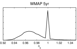
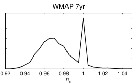
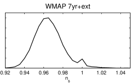
Figure 4: The model-averaged posterior distributions for the spectral index $n_{\rm s}$, using the WMAP 5yr data only (top), the WMAP 7yr data only (middle) and the WMAP 7yr+ext compilation (bottom). The probability distribution includes a delta function around $n_{\rm s}=1$, artificially broadened in the plot by the binning process. (From ref. [53])

Parkinson & Liddle [53] applied Bayesian model averaging to measurements of the parameters of the primordial power spectrum of density fluctuations. They considered five different models.

1. A scale-invariant Harrison–Zel’dovich (HZ) spectrum of scalar perturbations with no tensor component ($n_{\rm s}=1$, $r=0$).

2. A tilted model, where the spectral index is allowed to vary, still with no tensors.

3. A running model, where both the spectral index and the running of the spectrum ($n_{\rm run}$) are allowed to vary.

4. A tensor model, where the spectral index of the scalar perturbations and the tensor-to-scalar amplitude ratio ($r$) are allowed to vary.

5. A tensor+running model, where the spectral index, tensor-to-scalar ratio, and running all vary.

They also varied the physical baryon density $\Omega_{\rm b}h^{2}$, the physical CDM density $\Omega_{\rm c}h^{2}$, the angular diameter of the sound horizon at last scattering $\theta$, the optical depth to reionization $\tau$, the (log) amplitude of the density fluctuations, $\ln[10^{10}A_{\rm s}]$, and the amplitude of the Sunyaev–Zel’dovich contribution to the CMB power spectrum $A_{\rm SZ}$. They used data from the five-year and seven-year WMAP data releases, to compare how much improvement in model selection occurred between them, and also combined the seven-year WMAP with smaller-scale CMB experiments and measurements of the galaxy power spectrum by the Sloan Digital Sky Survey (SDSS).

The model-averaged posterior for $n_{\rm s}$ for the different data compilations are shown in Figure 4. When WMAP data alone was used, most of the models had similar evidence values, and so the averaged posterior had a substantial contribution from the delta-function from the HZ model. When the extra small scale and galaxy power spectrum data were added, the models where $n_{\rm s}$ was allowed to vary had larger evidence values, and these models also had posteriors for $n_{\rm s}$ that peaked for approximately the same values.

4.1.4 Summary

An interesting point to note is that in each of the above cases Bayesian model averaging was applied with a uniform model prior. That is, none of the authors felt that one model could be favoured a priori over the others. Because of the mysterious nature of these phenomena (dark energy, inflation) where any proposed physical mechanism is still highly speculative, the authors were forced to parameterize their ignorance with phenomenological descriptions. But since it is unknown even if these descriptions are accurately representing the real mechanism, no clear choice can be made in advance. This meant that the dimension of the models played the largest role in determining the evidence values, and so the model-averaged posteriors were dominated by the models with the fewest parameters. The exception to this was the primordial power spectrum case, where the simplest model (HZ) is close to being ruled out, and so its contributions to the model-averaged posterior are almost negligible.

4.2 Cluster weak lensing and Sunyaev–Zel’dovich effect data

The use of multiple models in a Bayesian framework is also useful in the case where the nature of the data is uncertain. One such case is galaxy clusters. Galaxy clusters are the largest gravitationally-bound objects in the Universe, and as such can be used as cosmological probes. However, the distribution of matter inside the cluster is crucial in recovering measurements of their properties, and often some model has to be assumed before probabilistic inferences on other cosmological parameters can be made.

Marshall et al. [12] applied Bayesian methods to the problem of cluster data modelling, attempting to fit the best model to the clusters’ gas and temperature profiles using simulated Sunyaev–Zel’dovich effect data and weak gravitational lensing data. They considered two models of the gas density profile, the ‘Beta’ model (see e.g. ref. [54]), and the full hydrostatic pressure equilibrium or ‘iHSE’ model. Both models assume a one-parameter isothermal temperature profile, and the only difference comes in the gas density distribution.

The Beta model has gas density profile

$$\rho_{\rm gas}(r)=\frac{\rho_{\rm gas}(0)}{\left[1+(r/r_{\rm c})^{2}\right]^{3\beta/2}}\,,$$ (17)

where $\rho_{\rm gas}(0)$ is a constant relating to the density at the centre of the cluster, $r_{\rm c}$ is the characteristic scale of the gas density profile, and $\beta$ is a parameter that gives the shape of the profile. This model is often used in cluster modelling.

In the iHSE model the gas is in full hydrostatic pressure equilibrium, with a potential defined by the NFW profile [55]. Solving for this potential, the gas profile is found to be

$$\rho_{\rm gas}=\rho_{\rm gas}(0)\exp\left[-\frac{4\pi G\rho_{\rm s}r_{{\rm s}}^{\prime 2}\mu}{kT}\left(1-\frac{\log(1+r/r_{\rm s})}{r/r_{\rm s}^{\prime}}\right)\right]\,,$$ (18)

where $G$ is Newton’s gravitational constant, $\mu$ is the mean mass per particle (here set to be 0.59), $k$ is the Boltzmann constant, and $T$ is the temperature. Finally $r_{\rm s}^{\prime}$ is the characteristic scale of the dark matter halo, as defined in the NFW profile. Note that the characteristic scale of the gas density in the Beta model ($r_{\rm s}$) and the characteristic scale of the dark matter density in the iHSE model ($r_{\rm s}^{\prime}$) are very different parameters and cannot really be directly compared.

They generated simulated data assuming contemporary facilities: observations of low-redshift clusters in the optical with MegaCam at CFHT, and at 30 GHz with the extended VSA [56]. They then went on to consider next-generation experiments, with mock lensing observations on the ESO Wide Field Imager and mock SZ data from AMI [57]. They used MCMC methods to fit the SZ data for $M_{\rm gas}$ and the weak gravitational lensing data for $M_{200}$, assuming uniform priors on both of these parameters. The ratio of these two gives the gas fraction of the cluster $f_{\rm gas}h$.

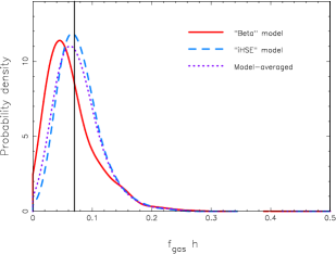
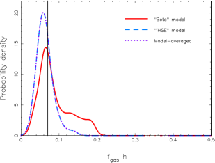
Figure 5: Marginalized probability distributions of cluster cosmological parameters from mock current (top) and future (bottom) experiments. The true cluster model is iHSE. $P(f_{{\rm gas}}h|D,{\rm Beta})$ and $P(f_{{\rm gas}}h|D,{\rm iHSE})$ are plotted with full and dashed lines respectively; the dotted curve shows the result of model averaging, $P(f_{{\rm gas}}h|D)$. In the next-generation case, the model-averaged curve is indistinguishable from the true model curve, as the evidence ratio between the two models is large. (From ref. [12])

The posterior distributions for the gas fraction parameter are shown in Figure 5. Using the current data, the evidence values of the two models were equal within the numerical errors, and so the model-averaged posterior is simply the average of the two posteriors. In contrast, when using next-generation data the evidence of the true model was much larger than that the incorrect model (though the precise numerical values depended on what was assumed about the primordial CMB contamination), and so the model-averaged posterior was indistinguishable from the true model posterior.

4.3 Distance measurements

The measurement of distances is another area in astrophysics where Bayesian methods are useful. Cepheid variable stars are established as distance indicators, but calibrating the Barnes–Evans Cepheid surface brightness relation [58] of these objects is still a challenge. Only relatively recently have interferometric measurements of their angular diameter allowed them to be calibrated geometrically, almost fully independent of all other astronomical distance scales [59].

Barnes et al. [60] applied Bayesian methods to this problem. They created an empirical model for the variation in magnitude with time (known as the light curve) and radial velocity with time, fitting them to Fourier polynomials of unknown order (here $M$ is the order of the velocity model and $N$ is the order of the magnitude model). Rather than fix the values of $M$ and $N$, they used Reversible Jump MCMC and let them vary. Each polynomial has amplitude and phase, and there is also a constant term, so the total number of parameters is $2M+1$ for the velocity data and $2N+1$ for the magnitude data. They also fit for the mean angular diameter, some hyperparameters relating to accuracy, an unknown phase shift between the magnitude and velocity variation and (most importantly) the distance. They put a uniform prior on the order of the Fourier polynomials, with a cut-off value.

They used an ensemble of thirteen Cepheids selected due to their high-quality photometry and availability of radial velocity data. They found for most of the Cepheids that more than one order had significant posterior probability (i.e. more than one value of $M$ or $N$ had significant evidence associated with it). They compared their results to the traditional method, where the order was selected ‘by eye’, usually with the criterion that the polynomial is terminated when the scatter in the polynomial approaches the uncertainty in the data. They found excellent agreement between the results from their method and those of the previous more traditional methodology.

4.4 Star Classification

The classification of objects has been a common application of Bayesian methods in astrophysics, where a model for the type of object can be selected using the evidence (for example see refs. [61] and [62]). Since the variables involved in the models are often very different, a model-averaging procedure does not necessarily lend itself to such problems. However, there are cases where the outputs of the different classification models can be combined in such a manner.

In ref. [63] the authors were interested in the fast classification of variable stars using neural networks. The intention is that this machine-learning approach can be applied to the large numbers of objects that will be detected by the CoRoT, Kepler, and Gaia satellite missions in an automated fashion. They use a multi-layer perceptron, but instead of using the maximum likelihood estimate from a single network, they use Bayesian Model Averaging to combine the output from a number of different networks, effectively using the networks as predictive models. They tested the Bayesian Averaging Artificial Neural Network approach against two other approaches, the $k$-dependent Bayesian Classifier [64] and the Support Vector Machines classifier [65]. They found that none of the methods particularly outperformed the others, all giving rather disappointing misclassification rates. The Bayesian Averaging Artificial Neural Network proved to be the exception in one case, that of the eclipsing binaries, achieving a correct classification rate of 99.73%.

This use of Bayesian Model Averaging is very interesting, as it illustrates how it can be applied in a situation where the underlying physical model is not known or well understood. In this case there is almost no physical model; the Artificial Neural Networks predict the brightness of the transients through empirical learning. Hence there is no prior belief about which model must be better than the other.

5 Conclusions

In this review we have summarised the application of Bayesian Model Averaging in a number of areas of astrophysics, namely cosmological model averaging for parameters associated with inflation and the dark energy, measurements of the baryonic gas fraction in galaxy clusters, calibrating accurate distances from Cepheid variable stars, and automated star classification using neural networks. We found that these applications fell broadly into one of two types, with model averaging being applied either in the case where the underlying physical model was uncertain, or the situation where some details about the data acquisition or modelling was uncertain. In all of these cases the model likelihood (evidence) was not able to discriminate between the different models, and so they all made some contribution to the averaged posterior.

There are still a number of research areas in astrophysics where Bayesian model averaging has not been implemented, even though Bayesian methods and model selection have been adopted. It is common for data to be unable to select a single preferred model; quoting parameter uncertainties based on selecting one particular model may then misrepresent the actual uncertainty, and can be directly addressed by Bayesian Model Averaging. Note that including model uncertainty does not necessarily increase the uncertainty on model parameters, e.g. tighter constraints are obtained on the dark energy equation of state if one includes the cosmological constant model, given its high evidence and fixed value of $w=-1$.

Areas we feel would benefit from the model-averaging approach include questions where the parameters of some signal have to be estimated in the presence of some unknown number of contaminating components. This would include, for example, gravitational wave astronomy and sub-millimetre and radio imaging surveys. Then there are cases where some data products are estimated with some model assumed, even though the evidence does not decisively select that model against other candidates, for instance orbital properties of extrasolar planets in systems where additional planets are marginally detected.

In Bayesian model averaging (as with any Bayesian method) the results have some dependence on the choice of model priors, especially as in the cases were model averaging is useful the model likelihoods will be similar. This should not deter the reader from applying such methods, as they simply require them to consider more deeply which models they consider more reasonable or likely before examining the data. Ultimately model averaging encodes and combines uncertainty at both the model and parameter level, and so provides a more complete description of the current state of knowledge.

References

- [1] D. J. C. MacKay, Information theory, inference, and learning algorithms, Cambridge University Press, Cambridge, 2003.
- [2] P. Gregory, Bayesian logical data analysis for the physical sciences, Cambridge University Press, Cambridge, 2005.
- [3] D. Sivia, J. Skilling, Data Analysis: A Bayesian Tutorial, 2nd edition, Oxford University Press, Oxford, 2006.
- [4] M. P. Hobson, A. H. Jaffe, A. R. Liddle, P. Mukherjee, D. Parkinson, Bayesian methods in Cosmology, Cambridge University Press, Cambridge, 2010.
- [5] R. E. Kass and A. E. Raftery, Bayes Factors, J. Am. Stat. Assoc., 90 (1995), 773-95.
- [6] H. Jeffreys, Theory of Probability (3rd ed.), Oxford: Oxford University Press, Oxford, 1961.
- [7] R. Trotta, Applications of Bayesian model selection to cosmological parameters, Mon. Not. Roy. Astron. Soc. 378 (2007) 72. arXiv:astro-ph/0504022.
- [8] A. Jaffe, H0 and Odds on Cosmology, Astrophys. J. 471 (1996) 24. arXiv:astro-ph/9501070.
- [9] P.S. Drell, T. J. Loredo, I. Wasserman, Type Ia Supernovae, Evolution, and the Cosmological Constant, Astrophys. J., 530 (2000), 593. arXiv:astro-ph/9905027.
- [10] M. V. John and J. V. Narlikar, Comparison of cosmological models using Bayesian theory, Phys. Rev. D, 65 (2002), 043506. arXiv:astro-ph/0111122.
- [11] A. Slosar et al., Cosmological parameter estimation and Bayesian model comparison using VSA data, Mon. Not. Roy. Astron. Soc., 341 (2003), L29. arXiv:astro-ph/0212497.
- [12] P. J. Marshall, M. P. Hobson, A. Slosar, Bayesian joint analysis of cluster weak lensing and sunyaev–zel’dovich effect data, Mon. Not. Roy. Astron. Soc., 346 (2003), 489. arXiv:astro-ph/0307098.
- [13] T. D. Saini, J. Weller, S. L. Bridle, Revealing the Nature of Dark Energy Using Bayesian Evidence, Mon. Not. Roy. Astron. Soc., 348 (2004), 603. arXiv:astro-ph/0305526.
- [14] A. Niarchou, A. H. Jaffe, L. Pogosian, Large-scale power in the CMB and new physics: an analysis using Bayesian model comparison, Phys. Rev. D, 69 (2004), 063515. arXiv:astro-ph/0308461.
- [15] B. A. Bassett, P. S. Corasaniti, M. Kunz, The essence of quintessence and the cost of compression, Astrophys. J. Letts., 617 (2004), L1. arXiv:astro-ph/0407364.
- [16] A. R. Liddle, P. Mukherjee, D. Parkinson, Cosmological Model Selection, Astronomy & Geophysics, 47 (2006), 4.30. arXiv:astro-ph/0608184.
- [17] R. Trotta, Bayes in the sky: Bayesian inference and model selection in cosmology, Contemp. Phys., 49 (2008), 71. arXiv:0803.4089 [astro-ph].
- [18] A. R. Liddle, Statistical methods for cosmological parameter selection and estimation, Ann. Rev. Nucl. Part. Sci., 59 (2009), 95. arXiv:0903.4210 [astro-ph].
- [19] J. A. Hoeting, D. Madigan, A. E. Raftery, C. T. Volinsky, Bayesian Model Averaging: A Tutorial, Statistical Sciences, 14.4 (1999), 382. Available at www.stat.washington.edu/www/research/online/ hoeting1999.pdf.
- [20] M H. Chen, Q-M. Shao, J. G. Ibrahim, Monte Carlo Methods in Bayesian Computation, Springer, New York, 2000.
- [21] N. Metropolis, A. W. Rosenbluth, M. N. Rosenbluth, A. H. Teller, E. Teller, Equation of State Calculations by Fast Computing Machines, Journal of Chemical Physics, 21 (1953), 1087.
- [22] W. K. Hastings, Monte Carlo sampling methods using Markov chains and their applications, Biometrika, 57 (1970), 97.
- [23] A. Lewis and S. Bridle, Cosmological parameters from CMB and other data: A Monte Carlo approach, Phys. Rev. D, 66 (2002), 103511. arXiv:astro-ph/0205436.
- [24] J. Skilling, Nested Sampling, in Bayesian Inference and Maximum Entropy Methods in Science and Engineering, ed. R. Fischer et al., Amer. Inst. Phys., conf. proc., Springer, New York, 735 (2004), 395. Available at http://www.inference.phy.cam.ac.uk/bayesys/.
- [25] J. Skilling, Nested sampling for general Bayesian computation, Bayesian Anal., 1 (2006), 833.
- [26] P. Mukherjee, D. Parkinson, A. R. Liddle, A Nested Sampling Algorithm for Cosmological Model Selection, Astrophys. J. Letts., 638 (2006), L51. arXiv:astro-ph/0508461v2.
- [27] F. Feroz, M. P. Hobson, M. Bridges, MultiNest: an efficient and robust Bayesian inference tool for cosmology and particle physics, Mon. Not. Roy. Astron. Soc., 398 (2009), 1601. arXiv:0809.3437 [astro-ph].
- [28] O. Cappé, A. Guillin, J.-M. Marin, C. P. Robert, Population Monte Carlo, J. Comp. Graph. Stats., 13 (2004), 907.
- [29] R. Douc, A. Guillin, J.-M. Marin, C. P. Robert, Convergence of adaptive mixtures of importance sampling schemes, Ann. Statist., 35 (2007), 420. arXiv:0708.0711 [math.ST].
- [30] S. Kullback and R. A. Leibler, On information and sufficiency, Annals of Mathematical Statistics, 22 (1951), 79.
- [31] M. Kilbinger, et al., Bayesian model comparison in cosmology with Population Monte Carlo, Mon. Not. Roy. Astron. Soc., 405 (2010), 2381. arXiv:0912.1614 [astro-ph].
- [32] O. Cappé, R. Douc, A. Guillin, J.-M. Marin, C. P. Robert, Adaptive importance sampling in general mixture classes, Stat. Comput., 18:4 (2008), 447.
- [33] P. J. Green, Reversible jump Markov chain Monte Carlo computation and Bayesian model determination, Biometrika, 82 (1995), 711.
- [34] M. Stephens, Bayesian analysis of mixture models with an unknown number of components an alternative to reversible jump methods, Ann. Statist., 28 (2000), 40 74.
- [35] O. Cappé, C. P. Robert , T. Rydén, Reversible jump, birth-and-death and more general continuous time Markov chain Monte Carlo samplers, J. Roy. Statstic. Soc. B, 65 (2003), 3, 679
- [36] N. J. Cornish, T. B. Littenberg, Tests of Bayesian Model Selection Techniques for Gravitational Wave Astronomy, Phys. Rev. D, 76 (2007), 083006. arXiv:0704.1808 [gr-qc]
- [37] A. Albrecht, et al., Report of the Dark Energy Task Force, 2006. Available: arXiv.org/abs/astro-ph/0609591.
- [38] A. R. Liddle, P. Mukherjee, D. Parkinson, Y. Wang, Present and future evidence for evolving dark energy, Phys. Rev. D, 74 (2006), 123506. arXiv:astro-ph/0610126.
- [39] E. V. Linder , Exploring the Expansion History of the Universe, Phys. Rev. Lett., 90 (2003), 091301. arXiv:astro-ph/0208512.
- [40] M. Chevallier and D. Polarski, Accelerating Universes with Scaling Dark Matter, Int. J. Mod. Phys. D, 10 (2001), 213. arXiv:gr-qc/0009008.
- [41] G. Hinshaw, et al. [WMAP collaboration], Three-Year Wilkinson Microwave Anisotropy Probe (WMAP) Observations: Temperature Analysis, Astrophys. J. Supp., 170 (2007), 288. arXiv:astro-ph/0603451.
- [42] D. N. Spergel, et al. [WMAP collaboration], Wilkinson Microwave Anisotropy Probe (WMAP) Three Year Results: Implications for Cosmology, Astrophys. J. Supp., 170 (2007), 377. arXiv:astro-ph/0603449.
- [43] M. Tegmark, et al., Cosmological Constraints from the SDSS Luminous Red Galaxies, Phys. Rev. D, 74 (2006), 123507. arXiv:astro-ph/0608632.
- [44] A. G. Riess, et al., Type Ia Supernova Discoveries at From the Hubble Space Telescope: Evidence for Past Deceleration and Constraints on Dark Energy Evolution, Astrophys. J., 607 (2004), 665. arXiv:astro-ph/0402512.
- [45] P. Astier, et al., “The Supernova Legacy Survey: Measurement of , and from the First Year Data Set”, Astron. & Astrophys., 447 (2006), 31. arXiv:astro-ph/0510447.
- [46] M. Vardanyan, R. Trotta, J. Silk, How flat can you get? A model comparison perspective on the curvature of the Universe, Mon. Not. Roy. Astron. Soc., 413 (2011), L91. arXiv:0901.3354 [astro-ph].
- [47] J. Dunkley, et al., [WMAP collaboration], Five-Year Wilkinson Microwave Anisotropy Probe (WMAP) Observations: Likelihoods and Parameters from the WMAP data, Astrophys. J. Supp., 180 (2009), 306. arXiv:0803.0586 [astro-ph].
- [48] W. J. Percival, S. Cole, D. J. Eisenstein, R. C. Nichol, J. A. Peacock, A. C. Pope, A. S. Szalay, “Measuring the Baryon Acoustic Oscillation scale using the SDSS and 2dFGRS, Mon. Not. Roy. Astron. Soc., 381 (2007), 1053. arXiv:0705.3323 [astro-ph].
- [49] M. Kowalski, et al., Improved Cosmological Constraints from New, Old and Combined Supernova Datasets, Astrophys. J., 686 (2008), 749. arXiv:0804.4142 [astro-ph].
- [50] R. Harrison, Fluctuations at the threshold of classical cosmology, Phys. Rev. D, 1 (1970), 2726.
- [51] Ya. B. Zel’dovich, A Hypothesis, Unifying the Structure and the Entropy of the Universe, Mon. Not. Roy. Astron. Soc., 160 (1972), 1p.
- [52] A. H. Guth, Inflationary universe: A possible solution to the horizon and flatness problems, Phys. Rev. D, 23 (1981), 347.
- [53] D. Parkinson, A. R. Liddle, Application of Bayesian model averaging to measurements of the primordial power spectrum, Phys. Rev. D, 82 (2010), 103533. arXiv:1009.1394 [astro-ph].
- [54] C. Sarazin, X-ray Emission from Clusters of Galaxies, Cambridge University Press, Cambridge, 1988.
- [55] J. F. Navarro, C. S. Frenk, S. D. M. White, A Universal density profile from hierarchical clustering, Mon. Not. Roy. Astron. Soc., 275 (1995), 720. arXiv:astro-ph/9408069.
- [56] K. Lancaster, et al., Very Small Array Observations of the Sunyaev–Zel’dovich effect in nearby galaxy clusters, Mon. Not. Roy. Astron. Soc., 359 (2005), 16. arXiv:astro-ph/0405582.
- [57] J. Zwart, et al., The Arcminute Microkelvin Imager, Mon. Not. Roy. Astron. Soc., 391 (2008), 1545.
- [58] T. G. Barnes, D. S. Evans, Stellar angular diameters and visual surface brightness - I. Late spectral types, Mon. Not. Roy. Astron. Soc., 174 (1976), 489.
- [59] T. E. Nordgren, B. F. Lane, R. B. Hindsley, P. Kervella, Calibration of the Barnes-Evans relation using interferometric observations of Cepheids, AJ, 123 (2002), 3380. arXiv:astro-ph/0203130.
- [60] T. G. Barnes, W. H. Jefferys, J. O. Berger , P. J. Mueller, K. Orr, R. Rodriguez, A Bayesian analysis of the cepheid distance scale, Astrophys. J., 592 (2003), 539; Erratum-ibid. Astrophys. J., 611 (2004), 621. arXiv:astro-ph/0303656.
- [61] M. P. Hobson, C. McLachlan, A Bayesian approach to discrete object detection in astronomical datasets, Mon. Not. Roy. Astron. Soc., 338 (2003), 765. arXiv:astro-ph/0204457.
- [62] R. Savage and S. Oliver S., Bayesian methods of astronomical source extraction, Mon. Not. Roy. Astron. Soc., 611 (2007), 1339. arXiv:astro-ph/0512597.
- [63] J. Debosscher, L. M. Sarro, C. Aerts, J. Cuypers, B. Vandenbussche, R. Garrido, E. Solano, Automated supervised classification of variable stars I. Methodology, Astron. & Astrophys., 475 (2007), 1159. arXiv:0711.0703 [astro-ph].
- [64] M. Sahami , Learning limited dependence Bayesian classifiers, in Second International Conference on Knowledge Discovery and Data Mining (Menlo Park, California: AAAI Press) (1996), 335
- [65] S. R. Gunn, M. Brown, K. M. Bossley, Network performance assessment for neurofuzzy data modelling, 1997, in IDA 97: Proceedings of the Second International Symposium on Advances in Intelligent Data Analysis, Reasoning about Data (London, UK: Springer–Verlag), 313.