Multi-phonon relaxation and generation of quantum states in a nonlinear mechanical oscillator

Abstract

The dissipative quantum dynamics of an anharmonic oscillator is investigated theoretically in the context of carbon-based nano-mechanical systems. In the short-time limit, it is known that macroscopic superposition states appear for such oscillators. In the long-time limit, single and multi-phonon dissipation lead to decoherence of the non-classical states. However, at zero temperature, as a result of two-phonon losses the quantum oscillator eventually evolves into a non-classical steady state. The relaxation of this state due to thermal excitations and one-phonon losses is numerically and analytically studied. The possibility of verifying the occurrence of the non-classical state is investigated and signatures of the quantum features arising in a ring-down setup are presented. The feasibility of the verification scheme is discussed in the context of quantum nano-mechanical systems.

1 Introduction

Nanoelectro-mechanical (NEM) resonators such as cantilevers, membranes and beams are important systems for the study of quantum phenomena in macroscopic, mechanical man-made objects [1]. For about a decade, the goal has been to cool the NEM resonators to the ground state and to verify the achievement of this state. This has recently been accomplished[2, 3, 4], and the next step is the generation, detection and coherent manipulation of more intricate quantum states, e.g., superpositions of macroscopic states (Schrödinger cat states) [5] and Fock states [6].

While a harmonic quantum oscillator displays a behavior analogous to its classical counterpart, the same does not hold for nonlinear oscillators. The presence of a conservative (Kerr) nonlinearity facilitates the creation of non-classical states. Although top-down fabricated NEM-resonators typically possess a finite Kerr constant $\mu$, it is usually too small to alone suffice for non-classical state generation. In contrast, carbon nanotubes (CNTs) and graphene membranes can exhibit strong enough nonlinearities for non-classical states to emerge during free evolution[7, 5]. Using CNTs or graphene also alleviates the need for active cooling due to their low masses and high frequencies[1, 5]. For this reason, carbon based NEM-resonators are highly promising for the study of nonlinear mechanical systems in the quantum regime.

If a system possesses conservative nonlinearities, it is natural to also take into account higher orders in the system-environment coupling. This results in nonlinear damping (NLD)[8, 9, 10, 11]. In carbon based NEM-resonators it has recently been shown that the dissipative mechanisms can indeed be nonlinear in the oscillator coordinate[12, 13]. Hence, to fully understand the quantum dynamics of carbon based NEM resonators it is essential to comprehend the interplay between conservative nonlinearities and NLD. In general, NLD will create interesting quantum features rather than remove them[14, 15, 16, 17, 18]. For example, as is well known in quantum optics[19, 16, 14, 15], for a harmonic oscillator, the steady state $\rho$ obtained from NLD due to two-photon losses at zero temperature ($T=0$) is a mixed state with $\rm{Tr}[\rho^{2}]<1$. Moreover, because of the parity conserving nature of the NLD, this steady state density matrix has coherences in terms of nonzero off-diagonal elements $\rho_{01}$ in the number basis. Recently, it was proposed to use this effect in order to generate and preserve Schrödinger cat states in a double well potential realized by a SQUID ring[18]. In an optomechanical setup non-thermal and squeezed states were shown to be obtainable by two-phonon cooling [20].

In this paper we study a situation more relevant to the coherent quantum dynamics of carbon based NEM-resonators, namely, a nonlinear oscillator with NLD. In this field there is little to be found in the literature[10]. Our main goals are to characterize the resulting steady states along with the corresponding features of the relaxation dynamics. For the nonlinear oscillator with NLD we find that the parity conserving nature of NLD helps to preserve phase coherence also in the presence of a finite conservative nonlinearity. However, we also find that for sufficiently large ratio between the Kerr constant $\mu$ and the NLD strength $\gamma_{2}$, the coherence of the steady state is suppressed. Further, at finite temperatures, with NLD, the final state is not a standard thermal state with a reduced density matrix $\rho\propto e^{-H/k_{B}T}$ unless linear damping (LD) is present. The corresponding Wigner distribution has a dip in the center, whose depth depends on the initial conditions. In the presence of both NLD and LD, the relaxation is governed by a crossover between two different relaxation rates. In the long-time limit, the decay rate $\Gamma$ is independent of the initial oscillator amplitude for NLD. Instead it is a function only of temperature $T$. To facilitate experimental determination of the governing damping mechanism, we also present the corresponding signatures in the time evolution of the position coordinate variance.

This paper is organized as follows: In section 2, we present the underlying theoretical frameworks used for analytical (rotating wave approximation [RWA]) and numerical (Wangsness-Bloch-Redfield[21, 22, 23]) calculations. The latter are used to verify the validity of the RWA-calculations. Then, in section 3, we present results pertaining to the steady states for various scenarios involving NLD and LD. Results on the relaxation towards the steady states are found in section 4, followed by a section with summary and conclusions.

2 Model and Methods

2.1 Model

To model the dynamics of the anharmonic oscillator subject to linear and nonlinear damping, we consider a single mechanical mode with frequency $\Omega$ and Kerr constant $\mu$. The mode is coupled linearly and nonlinearly to a reservoir of harmonic oscillators with mode frequencies $\omega_{k}$. The mode mass and the reduced Planck constant are set to be $m=1$ and $\hbar=1$, respectively. Correspondingly, the total Hamiltonian is H & = H_S+ H_B+ H_SB,
H_S = 12p^2+12Ω^2 q^2 + 2μ3q^4 ,
H_B = ∑_k ω_k b^†_k b_k,
H_SB = q ∑_k(2η_1 k)(b^†_k + b_k) + q^2 ∑_k(2 η_2 k) (b^†_k + b_k), where the mode position and momentum operators are $q=q_{0}(a^{{\dagger}}+a)/\sqrt{2}$, $p=\mathrm{i}(a^{{\dagger}}-a)/\sqrt{2}q_{0}$, and similarly the bath operators are given by $x_{k}=x_{0k}(b_{k}^{{\dagger}}+b_{k})/\sqrt{2}$, $p_{k}=\mathrm{i}(b_{k}^{{\dagger}}-b_{k})/\sqrt{2}x_{0k}$. Here $q_{0}=\sqrt{1/\Omega}$ and $x_{0k}=\sqrt{1/m_{k}\omega_{k}}$ are the zero point amplitudes of the oscillator and the bath, and satisfy the canonical commutation relations. The linear and the nonlinear coupling constants of the $k$’th reservoir mode to the resonator mode are denoted by $\eta_{1k}$ and $\eta_{2k}$, respectively. These couplings lead to amplitude-independent (linear) and amplitude-dependent (non-linear) [8, 9, 10, 11] damping of the oscillator motion. The former coupling involves the exchange of single vibration quanta (vibrons) with the reservoir, while in the latter case two vibrons are transferred simultaneously.

We consider the following scenario: The oscillator mode is assumed to be initially in the ground state $\left|0\right\rangle$. Then, by applying a voltage pulse for a finite time, the oscillator is displaced. The corresponding state is, by definition [24], a coherent state, $\Psi(t=0)=D(\alpha)\left|0\right\rangle\equiv\left|\alpha\right\rangle$. Here, $D(\alpha)=\exp(\alpha a^{\dagger}-\alpha^{*}a)$ is the displacement operator and the amplitude $\alpha$ depends on the strength and duration of the voltage pulse. During dissipation-free evolution under $H_{\rm S}$ only, a coherent state will evolve into a Yurke-Stoler cat state $(|\alpha\rangle+\rm i|-\alpha\rangle)/\sqrt{2}$. This state will periodically re-appear with a frequency set by the Kerr constant $\mu$. Typically the state’s emergence is slow compared to the system’s eigenfrequency $\Omega$ [25]. When taking into account the interaction with the reservoir, the created cat states will be influenced by the dissipation and the oscillator will eventually relax into a steady state. The state of the mechanical mode during the relaxation is described by the reduced density matrix (RDM) $\rho=\tr_{\rm B}\rho_{\rm T}$, which is obtained from the state of the total system $\rho_{\rm T}$ by tracing over bath degrees of freedom.

The time-evolution of the reduced density matrix is described by a (generalized) quantum master equation (QME) [26]. Here we follow the standard approach using the Born-Markov approximation to obtain the QME from the von Neumann equation for the total density matrix [26]. In this approximation the QME in the interaction picture with respect to $H_{\rm S}$ is given by

$$\frac{\partial}{\partial t}\rho(t)= -\sum_{l,m}\int_{0}^{\infty}d\tau\Big{[}A_{l}(t)A_{m}(t-\tau)\rho(t)-A_{m}(t-\tau)\rho(t)A_{l}(t)\Big{]}C_{lm}(\tau)$$ (1)

$$\>+\Big{[}\>\rho(t)A_{m}(t-\tau)A_{l}(t)-A_{l}(t)\rho(t)A_{m}(t-\tau)\Big{]}C_{ml}(-\tau).$$

The operators $A_{m}$ are given by the expansion of the interaction Hamiltonian in the interaction picture

$$H_{SB}=\sum_{m=1,2}A_{m}(t)\otimes B_{m}(t)\;,$$ (2)

where

$$A_{m}(t)=e^{\mathrm{i}H_{\rm S}t}\;(a^{{\dagger}}+a)^{m}\;e^{-\mathrm{i}H_{\rm S}t},\quad B_{m}(t)=\sum_{k}{q_{0}^{m}\eta_{mk}}\left(b^{{\dagger}}_{k}e^{\mathrm{i}\omega_{k}t}+b_{k}e^{-\mathrm{i}\omega_{k}t}\right).$$ (3)

Assuming the reservoir to be initially in thermal equilibrium, the reservoir correlation functions are given by

$$C_{ml}(\tau) = \tr_{B}\{B_{m}(t)B_{l}(t-\tau)\rho_{\rm B}\}$$ (4)

$$= \int\frac{d\omega}{2\pi}\kappa_{ml}(\omega)\left[n_{\rm B}(\omega)e^{\mathrm{i}\omega\tau}+(n_{\rm B}(\omega)+1)e^{-\mathrm{i}\omega\tau}\right]\;,$$

where $n_{\rm B}(\omega)=[e^{\omega/k_{\rm B}T}-1]^{-1}$ is the Bose distribution function, $\rho_{\rm B}$ is the thermal state and $\kappa_{ml}(\omega)=\kappa_{lm}(\omega)=2\pi\sum_{k}(\eta_{mk}\eta_{lk}q_{0}^{m+l})\delta(\omega-\omega_{k})$ is the spectral density of the environment coupling.

In general, the frequency dependence of $\kappa_{ml}$ is determined by the specific geometry of the system. As long as the spectral density is smooth and slowly varying around $\omega=\Omega$ and $\omega=2\Omega$ the detailed dependence on $\omega$ is not important[27] (see also 2.2). To be specific, we consider an Ohmic spectral density [26], i.e., we take

$$\kappa_{ml}(\omega)=\Gamma_{ml}\frac{\omega}{\Omega\sqrt{ml}}\;.$$ (5)

The values of $\Gamma_{11}$ and $\Gamma_{22}$ are used to specify the strength of LD and NLD, respectively. The off-diagonal value $\Gamma_{12}$ can, in general, be chosen independently of $\Gamma_{11}$ and $\Gamma_{22}$. If the oscillator couples to two independent baths, the off-diagonal spectral density vanishes. In the RWA, which is discussed in 2.2, the dissipation terms associated with $\Gamma_{12}$ can be neglected. Here we set $\Gamma_{12}=\sqrt{\Gamma_{11}\Gamma_{22}}$, which vanishes if either linear or nonlinear damping is absent.

2.2 Relaxation dynamics in the rotating frame

Typically, for NEMS the time scales associated with $\Omega$ and $\mu$ are well separated with $\Omega\gg\mu$ (see also section 5), which justifies an analytic treatment in the RWA. Within this approximation the QME (1) in the Schrödinger representation becomes[28]

$$\partial_{t}\rho(t)=(\mathcal{L}_{0}+\mathcal{L}_{1}+\mathcal{L}_{2})\rho(t),$$ (6)

where the Lindblad superoperators are given by

$$\begin{array}[]{lll}\mathcal{L}_{0}\rho&=&-i(\Omega+\mu)[a^{{\dagger}}a,\rho]-i\mu[(a^{{\dagger}}a)^{2},\rho],\\ \mathcal{L}_{1}\rho&=&\gamma_{-}a\rho a^{{\dagger}}-\frac{\gamma_{-}}{2}\{a^{{\dagger}}a,\rho\}+\gamma_{+}a^{{\dagger}}\rho a-\frac{\gamma_{+}}{2}\{aa^{{\dagger}},\rho\},\\ \mathcal{L}_{2}\rho&=&\gamma_{2-}aa\rho a^{{\dagger}}a^{{\dagger}}-\frac{\gamma_{2-}}{2}\{a^{{\dagger}}a^{{\dagger}}aa,\rho\}+\gamma_{2+}a^{{\dagger}}a^{{\dagger}}\rho aa-\frac{\gamma_{2+}}{2}\{aaa^{{\dagger}}a^{{\dagger}},\rho\}.\end{array}$$ (10)

The superoperators $\mathcal{L}_{0}$, $\mathcal{L}_{1}$ and $\mathcal{L}_{2}$ describe the coherent evolution due to $H_{\rm S}$, linear and the nonlinear interaction with the reservoir, respectively. The linear and nonlinear dissipation rates, $\gamma_{\pm}$ and $\gamma_{2\pm}$, are Fourier transforms of the correlation function (4), and are given by

$$\begin{array}[]{ll}\gamma_{+}=\Gamma_{11}n_{\rm B}(\Omega),&\gamma_{2+}=\Gamma_{22}n_{\rm B}(2\Omega),\\ \gamma_{-}=\Gamma_{11}[n_{\rm B}(\Omega)+1],&\gamma_{2-}=\Gamma_{22}[n_{\rm B}(2\Omega)+1].\end{array}$$ (13)

We would like to note, that the RWA equations given above are only valid for a weak nonlinearity[28]. This is reflected by the dependence of the rates on the transition frequency of the harmonic part of the Hamiltonian $H_{\rm S}$ and not on the frequencies of the full nonlinear $H_{\rm S}$. The validity of this approximation in the present case will be shown in the next sections by comparing to numerical calculations which include the exact transition frequencies (see also section 2.3).

The solution to (6) is obtained by rewriting the matrix equation as a set of decoupled equations. To this end, $\rho$ is projected onto the number basis $\rho_{n,n+\lambda}=\langle n|\rho|n+\lambda\rangle$, where $\lambda=0,1,2,\ldots$. It is convenient to define $\rho_{n,n+\lambda}(t)\equiv\sqrt{\frac{n!}{(n+\lambda)!}}\psi_{n}(\lambda,t)e^{\mathrm{i}\lambda(\Omega+\mu)t}$ [14], which also removes oscillations due to the term linear in $a^{\dagger}a$ in (6). For fixed $\lambda$ the function $\psi_{n}(\lambda,t)$ gives the entries of the $\lambda$’th super diagonal of $\rho$. Hence, (6) becomes

$$\partial_{t}\psi_{n}(\lambda,t) = \gamma_{2+}(n+\lambda)(n+\lambda-1)\psi_{n-2}+\gamma_{2-}(n+2)(n+1)\psi_{n+2}$$ (14)

$$-\{-\mathrm{i}\mu\lambda(\lambda+2n)+\gamma_{2-}n(n-1+\lambda)$$

$$+\frac{\gamma_{2-}}{2}\lambda(\lambda-1)+\gamma_{2+}(n+1)(n+2+\lambda)+\frac{\gamma_{2+}}{2}\lambda(\lambda+1)\}\psi_{n}$$

$$+\gamma_{-}(n+1)\psi_{n+1}+\gamma_{+}(n+\lambda)\psi_{n-1}$$

$$-\gamma_{-}(n+\frac{1}{2}\lambda)\psi_{n}-\gamma_{+}(n+1+\frac{1}{2}\lambda)\psi_{n}.$$

As indicated above, the equations for different $\lambda$ do not couple. In particular, for $\lambda=0$, we obtain a single equation for the populations $\rho_{n,n}(t)=\psi_{n}(0,t)$, which is used in the following to analyze the relaxation to the steady state.

In general, when all coefficients in (14) are non-zero the time evolution of $\psi_{n}(\lambda,t)$ has to be found numerically. If either $\gamma_{-}$ or $\gamma_{2-}$ is vanishing, i.e., there are only one or two vibron losses present, the time-dependence of $\psi_{n}(\lambda,t)$ can be calculated analytically (see [29, 30, 31] and [14]). In these cases it is also straight-forward to find the steady state solutions for all $\lambda$. An exact solution can also be obtained in terms of the positive P function where the nonlinear damping is equivalent to the real part of a complex Kerr constant [32]. At finite temperatures, when in addition to the losses, one or two vibron excitations ($\gamma_{\pm}>0$ or $\gamma_{2\pm}>0$) contribute, the stationary (time independent) probability distribution $\rho_{n,n}$ can be found using the detailed balance condition [33, 34] (see B). If one and two-vibron processes compete ($\gamma_{\pm}>0$ and $\gamma_{2\pm}>0$), a solution for $\rho_{n,n}$ can be given in terms of a continued fraction [35] or (for $\gamma_{2+}=0$) in terms of confluent hypergeometric functions[36].

In the next sections we are in particular interested in the behavior of the position variance

$$\left\langle\Delta q^{2}\right\rangle=\left\langle q^{2}\right\rangle-\left\langle q\right\rangle^{2}\;,$$ (15)

where $\left\langle\bullet\right\rangle=\tr_{\rm S}[\bullet\rho]$. Expressing $q$ in terms of creation and annihilation operators in the rotating frame one finds

$$\left\langle\Delta q^{2}\right\rangle/q_{0}^{2}\approx\frac{1}{2}\left[\left\langle a^{\dagger}a+aa^{\dagger}\right\rangle-2|\left\langle a^{\dagger}\right\rangle|^{2}\right]=\frac{1}{2}+\left\langle a^{\dagger}a\right\rangle-|\left\langle a^{\dagger}\right\rangle|^{2}\;,$$ (16)

where all oscillating contributions have been discarded. The expectation values of $a^{\dagger}a$ and $a^{\dagger}$ can be expressed in terms of $\psi_{n}(0,t)$ and $\psi_{n}(1,t)$, respectively,

$$\left\langle a^{\dagger}a\right\rangle = \sum^{\infty}_{n=0}n\,\rho_{n,n}=\sum^{\infty}_{n=0}n\,\psi_{n}(0,t)\;,$$ (17)

$$\left\langle a^{\dagger}\right\rangle = \sum^{\infty}_{n=0}\sqrt{n+1}\rho_{n,n+1}=\sum^{\infty}_{n=0}\psi_{n}(1,t)\;.$$ (18)

Knowing $\psi_{n}(0,t)$ and $\psi_{n}(1,t)$ therefore allows for an evaluation of the position variance. In the following we focus on obtaining such solutions in the long-time limit.

2.3 Numerical Computation

In order to investigate the oscillator dynamics and to verify the results obtained by the RWA approximation, the QME (1) is solved numerically by Wangsness-Bloch-Redfield [21, 22, 23] calculations. To this end the operators $A_{m}$ are represented in the eigenbasis of the oscillator Hamiltonian $H_{\rm S}$ and the Hilbert space is truncated after $30$ states ($40$ states for $\alpha=3$), which yields converged results. The initial coherent state, $\rho(0)=|\alpha\rangle\langle\alpha|$, is generated by applying the displacement operator $D(\alpha)$ to the ground state.

3 Steady state

3.1 Zero temperature

We begin with the RWA-analysis of the steady state $\rho(\infty)$ at zero temperature. To evaluate the applicability of the RWA, we compare the results to numerical calculations as described in section 2.3. If only single vibron losses are present in the system ($\gamma_{+}=0$, $\gamma_{2\pm}=0$), one finds from the equation of motion (14) for $\rho$ that any initial state $\rho(0)$ will decay to the ground state, i.e., $\rho(\infty)=|0\rangle\langle 0|$. The associated position variance is $\left\langle\Delta q^{2}\right\rangle/q_{0}^{2}=1/2$.

On the other hand, if only nonlinear losses are present ($\gamma_{2+}=0$, $\gamma_{\pm}=0$), a general initial state will relax to the steady state [14, 15]

$$\rho(\infty)=\rho_{0,0}|0\rangle\langle 0|+\rho_{0,1}|0\rangle\langle 1|+\rho_{1,0}|1\rangle\langle 0|+\rho_{1,1}|1\rangle\langle 1|,$$ (19)

where the matrix elements in (19) depend on the initial density matrix $\rho(0)$. Since for two-vibron losses parity is conserved, the only nonzero matrix elements on the main diagonal of $\rho(\infty)$ are

$$\rho_{0,0}(\infty) = \psi_{0}(0,\infty)=\sum_{n\>{\rm even}}\rho_{n,n}(0)\equiv P_{\rm even},$$ (20)

$$\rho_{1,1}(\infty) = \psi_{1}(0,\infty)=\sum_{n\>{\rm odd}}\rho_{n,n}(0)\equiv P_{\rm odd}\;.$$

The steady state off-diagonal elements $\rho_{0,1}$ and $\rho_{1,0}$ are in general non-zero and can also be found from a conservation law. From (14) one gets

$$\rho_{0,1}(\infty)=\rho_{1,0}^{*}(\infty)=\sum_{n=0}^{\infty}C_{2n}\psi_{2n}(1,0)e^{\mathrm{i}(\Omega+2\mu)t},$$

where the coefficients $C_{2n}$ are given in terms of Gamma functions (see A)

$$C_{2n}=\frac{\Gamma(\frac{1}{2}+n)\Gamma(1-\mathrm{i}\frac{\mu}{\gamma_{2-}})}{\sqrt{\pi}\Gamma(1+n-\mathrm{i}\frac{\mu}{\gamma_{2-}})}\;.$$ (21)

This expression is a generalization of the result of Simaan and Loudon [14] to the case of an anharmonic oscillator ($\mu\neq 0$). Note, that unless $\mu=0$, the off-diagonal element $\rho_{0,1}$ is time-dependent in the long time limit. Specifically, for a system which is initially in a coherent state $\left|\psi(t=0)\right\rangle=\left|\alpha\right\rangle$, i.e., with matrix elements

$$\rho_{n,m}(0)=\exp(-|\alpha|^{2})\alpha^{n}\alpha^{*m}/\sqrt{n!m!}\;,$$ (22)

the constants of motion are

$$P_{\rm even}=\exp(-|\alpha|^{2})\cosh(|\alpha|^{2})\;,$$

$$P_{\rm odd}=\exp(-|\alpha|^{2})\sinh(|\alpha|^{2})\;,$$

and

$$\psi_{\rm even}(t)\equiv\rho_{0,1}(\infty)=\alpha^{*}\exp(-|\alpha|^{2}-\mathrm{i}\mu t){}_{0}F_{1}(1-\mathrm{i}\frac{\mu}{\gamma_{2-}},|\alpha|^{4}/4)\;.$$ (23)

Here, ${}_{0}F_{1}$ is the confluent hypergeometric limit function [37]. For $\mu=0$ the latter becomes a Bessel function of the first kind and the expression given in [14] is recovered.

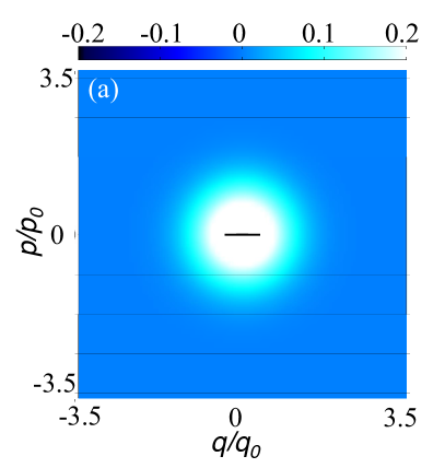
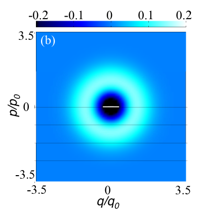
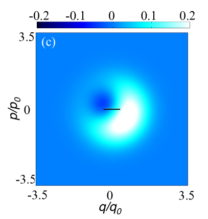
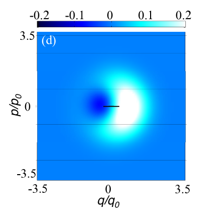
Figure 1: Wigner distributions (24) of the two lowest number states and typical steady states resulting from nonlinearly damped, initial coherent states with $\alpha=1$ at $T=0$. (a) Ground state $|0\rangle\langle 0|$. The black line indicates the size of the state given by $\sqrt{\left\langle\Delta q^{2}\right\rangle}/q_{0}=1/\sqrt{2}$. (b) First excited number state $|1\rangle\langle 1|$. The white line indicates the size of the ground state. (c) Weak NLD ($\gamma_{2-}/\mu=1/10$). The negative domains in the Wigner distribution reflect the presence of coherences (non-zero off-diagonals) in the steady state. For comparison the black line shows the size of the ground state. (d) Strong NLD ($\gamma_{2-}/\mu=10$). The black line is included for the same purpose as in (c).

To illustrate the differences between the numerically calculated states obtained by LD and NLD, their Wigner distributions [38]

$$W(q,p)=(2\pi)^{-1}\int d\xi~{}e^{-\mathrm{i}p\xi}\langle q+\xi/2|\rho(\infty)|q-\xi/2\rangle,$$ (24)

are displayed in figure 1. For comparison also the Wigner distributions of the ground and the first excited number state are included in figures 1 (a) and (b). While the ground state Wigner distribution is a Gaussian minimum uncertainty state, the first excited number state is a quantum state with negative domains in the Wigner distribution. The $\rho(\infty)$ resulting from NLD is a non-classical state with both negative and positive values in the Wigner distribution. This state is a mixed state which possesses coherences in terms of nonzero off-diagonal elements $\rho_{0,1}$ in the number basis (cf. (19)). In general it can be shown that the purity of this state is $\rm{Tr}[\rho^{2}]=1-2P_{even}P_{odd}+2|\rho_{0,1}|^{2}<1$. Figures 1 (c) and (d) display typical snapshots of this steady state for two different values of the ratio between the nonlinear damping rate and the Kerr constant. By comparing the sizes of the stationary states obtained by LD and NLD, it is seen that the latter occupy a larger phase-space area. This suggests, that the position variance $\langle\Delta q^{2}\rangle$ is suitable for quantifying the differences between the states resulting from these damping mechanisms.

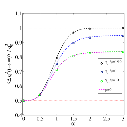
Figure 2: Zero temperature position variance of the steady state resulting from NLD as a function of the displacement amplitude $\alpha$ of the initial coherent state. The variance is averaged over one period $2\pi/\mu$. Dashed lines show the behavior according to (25) for different values of the ratio $\gamma_{2-}/\mu$. Symbols denote the corresponding numerical results. The lower dotted line (red) indicates the variance of the ground state, resulting from LD. The upper dotted line (gray) indicates the upper variance limit, resulting from weak NLD for $\alpha\rightarrow\infty$.

Using the definition (16) and the results above, one can evaluate the variance to be

$$\langle\Delta q^{2}(\alpha)\rangle_{T=0}/q_{0}^{2}=\frac{1}{2}+e^{-|\alpha|^{2}}\sinh(|\alpha|^{2})-|e^{-|\alpha|^{2}}\alpha^{*}{}_{0}F_{1}(1-\mathrm{i}\mu/\gamma_{2-},|\alpha|^{4}/4)|^{2}.$$ (25)

In figure 2, the variance according to (25) is shown as function of the displacement amplitude $\alpha$ of initial coherent states for different values of $\gamma_{2-}/\mu$ (dashed lines). The numerical results (symbols) are in accordance with (25). For comparison, also the variance of the ground state is included (red line), indicating its independence on the initial displacement amplitude. For small initial displacements, ($\alpha\lesssim 1$), the behavior of the variance is governed by the coherences $\rho_{0,1}=\rho_{1,0}^{*}$, since $\rho_{1,1}\to 0$. For large amplitudes, ($\alpha\gg 1$), and weak NLD, ($\gamma_{2-}\ll\mu$), the variance saturates at $1$ (gray dotted line). This is due to the ground and the excited states being equally populated, $\rho_{0,0}=\rho_{1,1}=1/2$, and the vanishing off-diagonal elements, since the hypergeometric function converges to zero. In the limit of strong NLD, ($\gamma_{2-}\gg\mu$), and large amplitudes, ($\alpha\gg 1$), the hypergeometric function converges to a non-zero value and the variance becomes $\left\langle\Delta q^{2}\right\rangle\to 1-1/2\pi$, which is larger than the variance of the ground state.

3.2 Finite temperature

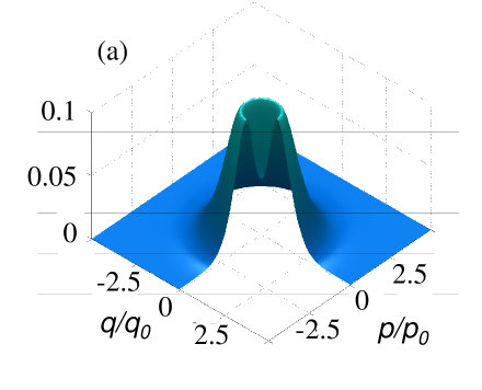
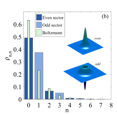
Figure 3: (a) Wigner distribution (24) of the stationary state resulting from NLD at finite temperature with parameters $\gamma_{2-}=\mu,~{}\alpha=1,~{}k_{\rm B}T/\Omega=1$. A sector of the Wigner distribution is cut out for a better visualisation of the dip in the middle, which indicates the difference to a regular thermal state. (b) Probability distribution of the even (dark blue bars) and odd (light blue bars) number state sectors of the stationary state shown in (a). The narrow bars represent the Boltzmann distribution of a thermal state described by (26). The insets show the Wigner distributions of the even and odd sectors, respectively.

Also at finite temperature $\rho(\infty)$ obtained by NLD will differ from the state obtained by LD. For LD only, $\rho(\infty)$ is fully characterized by the values of the diagonal matrix elements of the density matrix,

$$\rho_{n,n}=Z(\Omega)^{-1}e^{-n\Omega/(k_{\rm B}T)},$$ (26)

where $Z(\Omega)=\sum_{n}\exp[-n\Omega/(k_{\rm B}T)]$. Here, $k_{\rm B}$ is the Boltzmann constant and $T$ is the temperature of the bath. This result is found from (14) by taking $\lambda=0$ and setting the time-derivative to zero. One obtains the detailed balance condition, which leads to (26). As we have pointed out in section 2.2, the RWA equations (6) are valid for weak nonlinearities since the bath is only probed at the frequency $\Omega$. Consequently, at finite temperatures the stationary probability distribution calculated within the RWA will not depend on the Kerr constant. However, for sufficiently small temperatures, i.e., $\mu\left\langle a^{\dagger}a\right\rangle\ll\Omega+\mu$, the approximation is valid as we will also show in the following.

Since for nonlinear damping the two-vibron exchange conserves parity, one finds that detailed balance holds for each parity sector individually in this case. It can be shown (B) that

$$\rho_{2n,\>2n} = Z(2\Omega)^{-1}e^{-2n\Omega/(k_{\rm B}T)}P_{\rm even}\;,$$ (27)

$$\rho_{2n+1,\>2n+1} = Z(2\Omega)^{-1}e^{-2n\Omega/(k_{\rm B}T)}P_{\rm odd}\;.$$

Note that the stationary probability distribution at finite temperature also depends on the initial state. This implies that expectation values will in general also depend on $P_{\rm even}$ and $P_{\rm odd}$. For example, the average number of vibrons in the oscillator mode is given by

$$\left\langle a^{\dagger}a\right\rangle=\sum^{\infty}_{n=0}n\rho_{n,n}=2n_{\rm B}(2\Omega)+P_{\rm odd}\;,$$ (28)

which is derived in B.

Typical features of a stationary state obtained from nonlinear damping at finite temperature are displayed in figure 3. Figure 3 (a) shows the simulated Wigner distribution (see (24)), with parameters $\gamma_{2-}=\mu,~{}\alpha=1,~{}k_{\rm B}T/\Omega=1$. A sector is cut out for better visualisation of its features. As discussed in section 3.2, the thermal probability distribution of a nonlinearly damped state is split into an odd and an even parity sector. Each of the sectors has a Boltzmann-like distribution (see (27)). The shape of the Wigner distribution reflects this parity dependence by having a dip centered at the origin. It can be shown that $W(0,0)=(P_{\rm even}-P_{\rm odd})/2\pi$. Therefore, the dip in the Wigner distribution only depends on the initial state and not on temperature. Hence, in the case of an initial coherent state $|\alpha\rangle$, the dip will only depend on the initial oscillator displacement. For large displacement amplitudes the difference between the sectors becomes smaller, and $W(0,0)\rightarrow 0$. If the initial state had an odd parity, the dip of the Wigner distribution would attain a negative value.

Figure 3 (b) shows the Boltzmann-like distributions of the odd and the even sectors of the stationary state discussed above. The narrow bars represent the distribution of the thermal state obtained by linear damping (see (26)). The insets show the Wigner distributions of the even and odd sectors.

As the Wigner distribution of the finite temperature stationary state displays quantum signatures, so does its variance. Figure 4 shows the stationary state variance as function of the displacement amplitude $\alpha$ of the initial coherent state for several temperatures ($k_{\rm B}T/\Omega\in[0,1/4,1/2,3/4,1]$ and $\gamma_{2-}=\mu$). Dashed lines correspond to the analytical expression given by (37). Numerical calculations (symbols) are shown for the same parameters. The variance is seen to always be larger than the zero temperature variance, displayed in figure 2. This is due to an additional contribution from the Boltzmann distribution and the vanishing off-diagonal elements of the density matrix (see section 4.3). The variance is still dependent on the initial displacement and saturates at $\langle\Delta q^{2}\rangle/q_{0}^{2}=1+2n_{\rm B}>1$ for large $\alpha$, which is in contrast to $k_{\rm B}T/\Omega=0$ for which $\langle\Delta q^{2}\rangle/q_{0}^{2}\leq 1$.

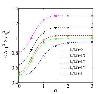
Figure 4: Finite temperature position variance of the stationary state as a function of the displacement amplitude $\alpha$ of the initial coherent state. The variance is averaged over one period $t=2\pi/\mu$. Dashed lines show the behavior according to (37) for $\gamma_{2-}=\mu$ and different temperatures. Symbols denote the corresponding numerical results.

4 Relaxation Dynamics

4.1 Zero temperature, NLD

We now investigate the relaxation dynamics of initial coherent states which evolve into the steady states discussed in the previous section. Figure 5 (a) shows the numerically calculated variance $\langle\Delta q^{2}\rangle$ as function of rescaled time $\tau=\mu t/\pi$ for several values of the ratio $\gamma_{2-}/\mu$. The variance is sampled at multiples of the period $\Omega/(2\pi)$, and therefore fast oscillations are not seen. For weak NLD ($\gamma_{2-}/\mu\lesssim 10$), the short time dynamics ($\tau\lesssim 1$) is governed by the Kerr constant $\mu$. This is reflected in the initial increase of variance. The maximum variance, at which the Yurke-Stoler cat state is first expected to appear [25, 5], is attained at $\tau\approx 1/2$. The variance of this state is given by $\langle\Delta q^{2}\rangle_{\rm cat}=q_{0}^{2}(4\alpha^{2}+1)/2$, which is always larger than the variance of a coherent state for a nonzero $\alpha$. As seen in the figure 5 (a), the shape of the variance peaks changes in time as the cat states decohere by NLD. Figure 5 (b) shows the Wigner distribution sampled at $\tau=1/2$, displaying a cat state under influence of NLD. Some of its original features are still visible, like the remnants of the negative interference domains.

After $\tau=1$, the system gradually relaxes to the state (19). In figure 5 (a) this is reflected by steady oscillations around a mean value of $\langle\Delta q^{2}\rangle$ which is, as discussed in section 3.1, larger than $1/2$. The oscillations in $\langle\Delta q^{2}\rangle$ are caused by the complex valued, oscillating coherences of $\rho_{0,1}$. The relaxation dynamics described above becomes faster with increasing ratio $\gamma_{2-}/\mu$. Figure 5 (c) shows the Wigner distribution of the state sampled at $\tau=11/2$, where the resemblance to the steady state in figure 1 (c) is clearly seen.

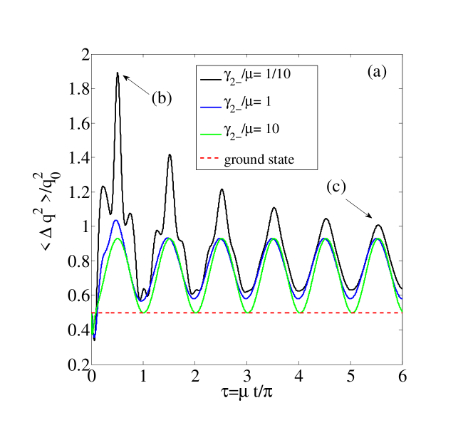
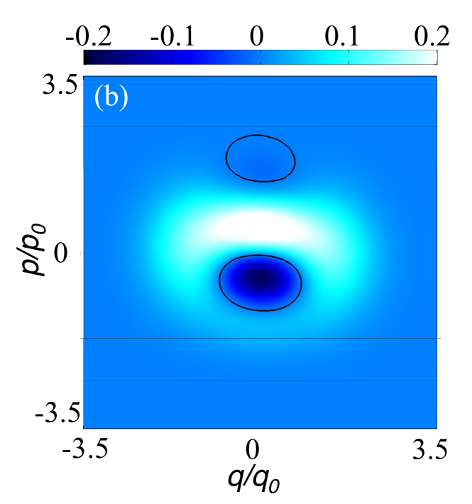
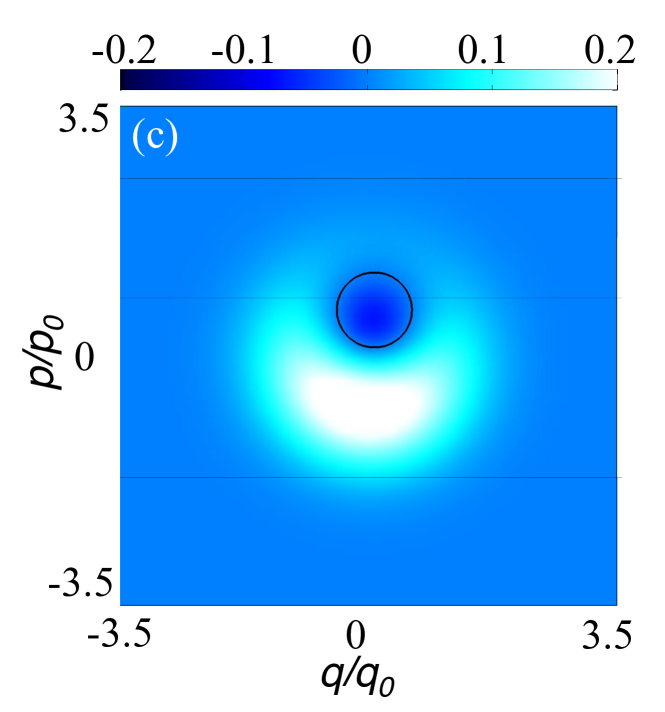
Figure 5: (a) Time evolution of the position variance of an initial coherent state with $\alpha=1$ at $T=0$ for different NLD strengths. The dashed line (red) indicates the variance of the ground state. (b) Wigner distribution $W(q,p)$ of the decohered Yurke-Stoler cat state attained at $\tau=1/2$. (c) Wigner distribution $W(q,p)$ of the state in (b) at a later time, $\tau=11/2$, reaching the steady state. Black contours encircle domains where $W<0$.

4.2 Zero temperature, LD and NLD

As shown in the previous section, NLD at $T=0$ leads to the formation of the non-classical state (19). In the additional presence of LD the generation of this state will be affected and eventually the ground state will be reached. In the following we discuss the resulting decay of the variance, which can be used to extract information about the nature of the damping mechanism and the state initially created by NLD.

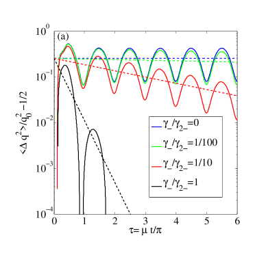
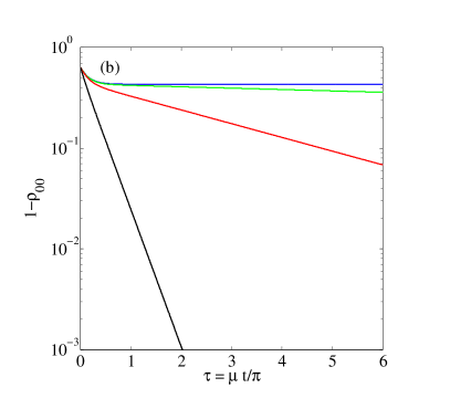
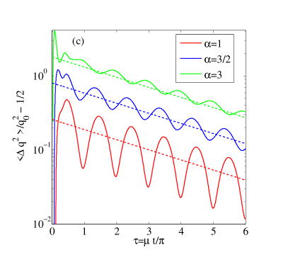
Figure 6: (a) Time-dependence of the position variance of a linearly and nonlinearly damped mechanical mode for $\alpha=1$ and $\gamma_{2-}=\mu$. Full lines denote different values of $\gamma_{-}/\gamma_{2-}$. Dashed lines show the function (31). (b) Time-dependence of $(1-\rho_{0,0})$ with parameters corresponding to those of the main figure. (c) Time dependence of $\langle\Delta q^{2}(\tau)\rangle/q_{0}^{2}-1/2$ for $\gamma_{2-}=\mu$ and $\gamma_{-}/\gamma_{2-}=1/10$ for different initial displacement amplitudes. Dashed lines indicate the behavior according to (31). For visual convenience, the graphs corresponding to $\alpha=3$ are multiplied by a factor of $2$.

We introduce the ratio $\gamma_{-}/\gamma_{2-}$ as a measure of the relative dissipation strength, and set $\gamma_{2-}=\mu$.

In presence of LD at $T=0$, (14) leads to (for $\lambda=0,1$)

$$\frac{\partial}{\partial t}\rho_{n,n}(t) = \gamma_{-}(n+1)\rho_{n+1,n+1}+\gamma_{2-}(n+2)(n+1)\rho_{n+2,n+2}$$ (29)

$$-\left[\gamma_{2-}n(n-1)+\gamma_{-}n\right]\rho_{n,n}\;,$$

$$\frac{\partial}{\partial t}\psi_{n}(1,t) = \gamma_{-}(n+1)\psi_{n+1}+\gamma_{2-}(n+2)(n+1)\psi_{n+2}$$ (30)

$$-\left[-\mathrm{i}\mu(1+2n)+\gamma_{2-}n^{2}+\gamma_{-}(n+\frac{1}{2})\right]\psi_{n}\;.$$

It is seen that only $\rho_{0,0}$ is non-zero in the stationary limit, i.e., $\rho_{1,1}$ and $\psi_{n}$ decay for sufficiently large times. In the limit of strong NLD, $\gamma_{-}\ll\gamma_{2-}$, one finds that the populations $\rho_{n,n}$ for $n>1$ rapidly decay due to two-vibron losses, but $P_{1}$ is only decreased via one-vibron losses. Hence, $\dot{\rho}_{1,1}\approx-\gamma_{-}\rho_{1,1}$ and $\rho_{1,1}(t)\approx e^{-\gamma_{-}t}P_{\rm odd}$. Here it is assumed that the initial decay on the time-scale $1/\gamma_{2-}$ is not influenced by the LD and $\rho_{0,0}(0)\approx P_{\rm even}$ and $\rho_{1,1}(0)\approx P_{\rm odd}$. Similarly, one finds that $\psi_{0}(1,t)\approx\exp[(\mathrm{i}\mu-\gamma_{-}/2)t]\psi_{\rm even}(0)$. Therefore, the position variance will decay to the minimum uncertainty value $1/2$ according to

$$\left\langle\Delta q^{2}\right\rangle/q_{0}^{2}=\frac{1}{2}+\left[P_{\rm odd}-|\psi_{\rm even}(0)|^{2}\right]e^{-\gamma_{-}t}\;.$$ (31)

Figure 6 (a) shows the time evolution of the numerically calculated $\langle\Delta q^{2}\rangle$ for different values of the ratio $\gamma_{-}/\gamma_{2-}$ and $\mu=\gamma_{2-}$. For $\gamma_{-}/\gamma_{2-}\lesssim 1/10$, the evolution of the variance for short times $\tau\lesssim 1$ resembles the result shown in figure 5. The short-time dynamics is again influenced by the Kerr constant, while the long-time behavior, ($\tau\gg 1$) is showing the relaxation of the state created by NLD. In this stage the variance is exponentially decaying with the decay being faster for larger values of $\gamma_{-}/\gamma_{2-}$. In figure 6 (b) the time evolution of $(1-\rho_{0,0})$ is shown, confirming the decay to the ground state. The parameters are the same as in 6 (a). For equally strong LD and NLD, ($\gamma_{-}=\gamma_{2-}$), an exponential decay is seen for the entire time interval. For LD weaker than NLD, ($\gamma_{-}<\gamma_{2-}$) and $\tau\lesssim 1/2$, the decay is initially not exponential, whereas for $\tau\gtrsim 1$ the ground state population displays exponential increase.

Figure 6 (a) suggests the concept of sequential relaxation for weak LD. The first stage of the sequence ($0<\tau\lesssim 1$), is mainly dominated by NLD and the Kerr constant, which leads to the formation of the state in (19). The second stage ($\tau\gtrsim 1$), is mainly influenced by the relaxation to the ground state because of LD. In other words, the state in (19) is initially created by NLD, and then decays due to LD. Accordingly, the average variance in the second relaxation stage is expected to be given by (31), which is displayed in figure 6 (a) (dashed lines). It can be seen that the idea of sequential relaxation is quantitatively correct for $\gamma_{-}\ll\gamma_{2-}$. Furthermore, (31) implies that the decay rate, which is equal to $\gamma_{-}$, is independent of the initial amplitude $\alpha$. This is shown in figure 6 (c) where the time evolution of $\langle\Delta q^{2}(\tau)\rangle$ is plotted for $\alpha=1,~{}3/2$ and $3$ ($\gamma_{2-}=\mu$, $\gamma_{-}/\gamma_{2-}=1/10$).

4.3 Finite temperature, NLD

While at $T=0$ two-vibron losses facilitate the creation of the non-classical state (19), thermal two-vibron excitations will contribute to its decoherence. From (14) one sees that a finite rate $\gamma_{2+}$ couples the states ($n=0,1$) to other excited states. These thermal excitations will eventually destroy the coherence of the non-classical states and the off-diagonal matrix elements will vanish. To quantify this decay we consider low temperatures, such that $\gamma_{2+}\ll\gamma_{2-}$. To obtain the relaxation rate to lowest order in $\gamma_{2+}$ it is sufficient to study excitations from $n=0$ to $n=2$. Consequently, one gets from (14) the coupled equations

$$\dot{\psi}_{0}(1,t) = (\mathrm{i}\mu-4\gamma_{2+})\psi_{0}+2\gamma_{2-}\psi_{2},$$ (32)

$$\dot{\psi}_{2}(1,t) = 6\gamma_{2+}\psi_{0}+(5\mathrm{i}\mu-16\gamma_{2+}-4\gamma_{2-})\psi_{2}\;,$$

supplemented by initial conditions for $\psi_{0}(1,0)$ and $\psi_{2}(1,0)$. For small $\gamma_{2+}$ we can assume that these initial values correspond to the values of the state in (19), which is the steady state solution for $\gamma_{2+}=0$. This amounts to setting

$$\psi_{0}(1,t=0)=\psi_{\rm even}(0),\quad\psi_{2}(1,t=0)=0\;.$$ (33)

The system (32) can be solved for $\psi_{0}(1,t)$,

$$\psi_{0}(1,t) = \Big{[}\cosh(2\chi t)+\Big{(}\frac{3\gamma_{2+}-\mathrm{i}\mu+\gamma_{2-}}{\chi}\Big{)}\sinh(2\chi t)\Big{]}$$

$$\times\exp[-(2\gamma_{2-}+10\gamma_{2+}-3\mathrm{i}\mu)t]\psi_{\rm even}(0)\;,$$

where $\chi=[\gamma_{2-}^{2}+(3\gamma_{2+}-\mathrm{i}\mu)^{2}+\gamma_{2-}(9\gamma_{2+}-2\mathrm{i}\mu)]^{1/2}$. Equation (4.3) describes the relaxation of a non-classical state due to weak thermal excitations. The relaxation rate, which is determined by $\chi$, depends on the strength of the Kerr constant $\mu$ and temperature via $\gamma_{2\pm}$. It is interesting to consider the limiting cases of strong and weak NLD. For strong NLD, $\gamma_{2-}/\mu\rightarrow\infty$, one finds $\chi\rightarrow\gamma_{2-}+(11\gamma_{2+})/2$ and $\psi_{0}(1,t)$ becomes

$$\psi_{0}(1,t)\simeq\psi_{0}(1,0)e^{-\gamma_{2+}t}.$$ (35)

Similarly, for weak NLD, $\gamma_{2-}/\mu\rightarrow 0$, $\chi\rightarrow-\mathrm{i}\mu+4\gamma_{2+}+\gamma_{2-}$ and the time evolution is

$$\psi_{0}(1,t)\simeq\psi_{0}(1,0)e^{(\mathrm{i}\mu-4\gamma_{2+})t}.$$ (36)

Obviously, the decoherence rate increases with increasing strength of the Kerr constant. This can be understood from the fact that the accumulated phase shift in the excited state is proportional to $\mu$. Therefore, for finite $\mu$ there is an additional dephasing, which contributes to the decay of $\psi_{0}(1,t)$. Altogether, the position variance becomes

$$\left\langle\Delta q^{2}\right\rangle/q_{0}^{2}\approx\frac{1}{2}+2n_{\rm B}(2\Omega)+P_{\rm odd}+|\psi_{0}(1,t)|^{2}\;.$$ (37)

Figure 7 (a) shows the time dependence of the numerically calculated variance for the same parameters as in figure 3 (d) with the initial displacement amplitude $\alpha=1$. The $T=0$ variance is included as a reference (blue) and is almost identical to the curve for $k_{\rm B}T/\Omega=1/4$ (green). When comparing the graphs in figure 7 (a) with figure 5 (a) and 6 (a), one finds a qualitatively similar behavior. It is seen that also for finite temperatures the relaxation proceeds sequentially. The short-time dynamics show an increase in variance, corresponding to the formation of a Schrödinger cat state. For longer times the variance is increasing with time, and the rate of approaching the stationary value is faster for larger temperatures.

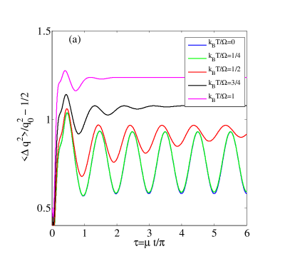
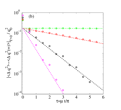
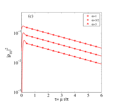
Figure 7: (a) Time dependence of the position variance of the nonlinearly damped mechanical mode at finite temperature for the same parameters as in figure 4. (b) Time dependence of $|\langle\Delta q^{2}(\tau)\rangle-\langle\Delta q^{2}(\infty)\rangle|_{T>0}$ for parameters $\alpha=1$, $\mu=\gamma_{2-}$, $\gamma_{-}=0$ and $k_{\rm B}T/\Omega\in[1/4,1/2,3/4,1]$. Symbols denote numerical results averaged over one period of and dashed lines show the behavior according to (39). (c) Time dependence of $|\rho_{0,1}(\tau)|^{2}$ at $k_{\rm B}T/\Omega=1/2$ for $\alpha=1$ ($\circ$), $\alpha=3/2$ ($\square$) and $\alpha=3$ ($\triangle$). The long-time limit relaxation rate is according to (38).

In order to quantify the finite temperature relaxation rate, the time evolution of $|\langle\Delta q^{2}(\tau)\rangle-\langle\Delta q^{2}(\infty)\rangle|_{T>0}$ is shown in Figure 7 (b), where the stationary state variance $\langle\Delta q^{2}(\infty)\rangle_{T>0}$ is subtracted from $\langle\Delta q^{2}(\tau)\rangle_{T>0}$ in order to remove the finite asymptotic value. The numerically obtained variance (symbols) is averaged over one period $t=2\pi/\mu$, which removes the oscillations due to the finite Kerr constant $\mu$. The temperatures are the same as in figure 7 (a). The figure confirms the idea of different relaxation stages, with the decay in the second stage being exponential and the rate being temperature dependent.

For comparison, figure 7 (c) shows the time evolution of $|\rho_{0,1}(\tau)|^{2}$ for $k_{\rm B}T/\Omega=1/2$ and $\alpha\in[1,3/2,3]$. It can be seen that in the long-time limit the decay rates do not depend on the initial oscillator displacement $\alpha$. As discussed above, the off-diagonal matrix elements $\rho_{0,1}$ decay due to thermal excitations. For low temperatures, their evolution is given by (4.3). When the Kerr constant and the NLD are equally strong, ($\mu=\gamma_{2-}$), one finds $\chi\rightarrow\gamma_{2-}+(19\gamma_{2+})/4-\mathrm{i}(\mu-3\gamma_{2+}/4)$ and the time evolution is given by

$$\psi_{0}(1,t)\simeq\psi_{0}(1,0)e^{\mathrm{i}(\mu+3\gamma_{2+}/2)t}e^{-(5\gamma_{2+}/2)t}.$$ (38)

The resulting behavior is shown in figure 7 (c) and it can be seen that (38) correctly describes the decay of $\rho_{0,1}$. From figures 7 (a) and (b) it can be concluded that the variance increase is mainly due to the decay of $|\rho_{0,1}|^{2}$. Consequently, we make the Ansatz

$$|\langle\Delta q^{2}(\infty)\rangle_{T>0}-\langle\Delta q^{2}(t)\rangle|_{T>0}=q_{0}^{2}|\psi_{0}(1,0)|^{2}e^{-\Gamma t},$$ (39)

which will be valid in the second stage of the relaxation. From (38) we find $\Gamma(T)\approx 5\gamma_{2+}(2\Omega)$. This Ansatz is displayed in figure 7 (b) (dashed lines) and a good quantitative agreement with the numerical results is found for all temperatures. Using (39) one can therefore infer the value of $|\rho_{0,1}|^{2}$ at the end of the first relaxation stage, which is dominated by the NLD. This allows for a reconstruction of the properties of the non-classical state (19), which is created at the end of the first relaxation stage.

4.4 Finite temperature, LD and NLD

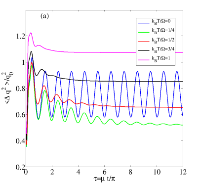
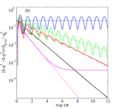
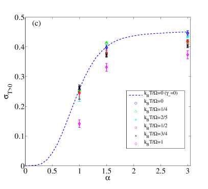
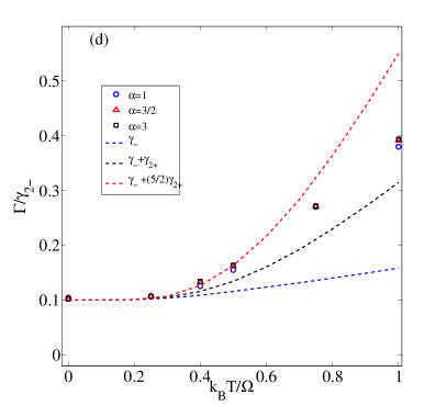
Figure 8: (a) Time-dependence of the position variance of an initial coherent state with $\alpha=1$, at different temperatures with NLD ($\gamma_{2-}=\mu$) and LD ($\gamma_{-}/\gamma_{2-}=1/10$). (b) Time dependence of $|\langle\Delta q^{2}(\tau)\rangle-\langle\Delta q^{2}(\infty)\rangle|_{T>0}$. The dashed lines indicate a fit of (40) to the numerical data. (c) and (d) Extracted fit parameters $\sigma$ and $\Gamma$ as functions of initial displacement amplitude $\alpha$ and temperature, respectively. The dashed line in (c) shows the variance according to (25) for $T=0$ and $\gamma_{-}=0$.

Finally, in this section we consider the time evolution of the position variance at finite temperature under influence of both LD and NLD. Figure 8 (a) shows the time-dependence of the numerically obtained $\left\langle\Delta q^{2}\right\rangle$ for $\gamma_{2-}=\mu,~{}\gamma_{-}/\gamma_{2-}=1/10,~{}\alpha=1$ and different temperatures. The behavior for $T=0$, which corresponds to setting $\gamma_{-}=0$, is included for reference (blue). As in the previous section we subtract the stationary state variance from $\left\langle\Delta q^{2}\right\rangle$ to study the relaxation towards the stationary state. This is shown in figure 8 (b). For long times an exponential decay is seen for temperatures $k_{\rm B}T/\Omega<1$. To quantify the decay we use the Ansatz in (39) and consider

$$|\langle\Delta q^{2}\rangle-\langle\Delta q^{2}(\infty)\rangle|_{T>0}=q_{0}^{2}(\sigma-\frac{1}{2})e^{-\Gamma t},$$ (40)

where $\sigma$ and $\Gamma$ are estimated by a least-square fit to the numerical data. To this end the variance is averaged over one period $t=2\pi/\mu$ which removes the oscillations due to the finite Kerr constant $\mu$. The fitting for $T\leq 3/4$ is done for the time interval $3<\tau<11$ and for $T=1$ in the time interval of $2<\tau<4$. The resulting behavior of (40) is displayed as dashed lines in figure 8 (b).

In figures 8 (c) and (d) the extracted parameters $\sigma$ and $\Gamma$ are shown as functions of initial displacement amplitude $\alpha$ and temperature, respectively. Due to the sequential relaxation, the parameter $\sigma$ approximately corresponds to the variance of the non-classical state (19), which is created in the initial stage. The analytic expression for $T=0$, given by equation (25), is shown in figure 8 (c) for comparison. The extracted low temperature results are in good agreement with the analytic curve. For higher temperatures deviations from the analytic behavior can be seen. However, the qualitative dependence on the initial amplitude is still similar to the one given by (25).

In figure 8 (d) the temperature dependence of the extracted decay rates $\Gamma$ is compared to the rates of one-vibron loss $\gamma_{-}$ and two-vibron excitations $\gamma_{2+}$, which determine the decay rate in the situations investigated in sections 3.2 and 4.2. It can be seen, that also in the present case the decay rate is independent of the initial coherent state displacement amplitude. For low temperatures, $k_{\rm B}T/\Omega<0.3$, one-vibron loss is the dominating damping mechanism. For higher temperatures the interplay of one-vibron and two-vibron processes leads to a more complicated behavior. At first the rate follows the behavior given by the combined rates $\gamma_{-}+5\gamma_{2+}/2$ but starts to deviate at $k_{\rm B}T/\Omega\approx 0.3$. With increasing temperature it stays between $\gamma_{-}+\gamma_{2+}$ and $\gamma_{-}+5\gamma_{2+}/2$.

The results presented in this section show that a ring-down measurement of the variance can be used to identify the quantum features of an initially created non-classical state, provided the sequential relaxation regime can be accessed. Moreover, the analysis of the decay rates can provide information about the dominating dissipation mechanisms in the system under investigation.

5 Summary and conclusions

In this work we have investigated a nonlinear oscillator in the quantum regime. The system is subject to nonlinear damping (two-vibron exchange), which resembles the two-photon decay known from quantum optics. The initially displaced oscillator relaxes to a steady state, which is determined by the relative strength of the linear and the nonlinear damping mechanisms and the temperature of the thermal bath. For sufficiently strong NLD we find that the relaxation is sequential: In the first stage, the initial density matrix decays to a non-classical state (19), followed by the second stage, where this state further decays to the final steady state. The non-classical state depends on the initial state, while the decay rates depend on temperature and the strength of LD and NLD.

At zero temperature, the sequential relaxation allows for a reconstruction of the properties of the non-classical state even in the presence of LD, i.e., when the stationary state is always the ground state. This can be achieved by performing a ring-down measurement of the position variance. For finite temperatures, NLD and thermal excitations lead to a different steady state - a stationary thermal state with a parity dependent Boltzmann-like distribution (27). The parity dependence is a signature of the NLD at finite temperatures. In the sequential relaxation regime the properties of the non-classical state can again be extracted from variance measurements.

In the following we briefly discuss the possibility of observing the relaxation of the non-classical state (19) in experiments with carbon-based nanomechanical resonators. A recent experiment [12] indicates significant NLD in micrometer sized, carbon-based resonators (nanotubes and graphene) with resonance frequencies of several hundreds of MHz. These systems are nonlinear and can be described by the classical Duffing equation of motion [39]

$$m\ddot{q}=-m\Omega^{2}q-\alpha_{0}q^{3}-\gamma\dot{q}-\eta q^{2}\dot{q},$$ (41)

where $q$ is the oscillator position, $m$ and $\Omega$ are the oscillator mass and frequency, $\alpha_{0}$ is the nonlinearity strength, $\gamma$ is the LD rate and $\eta$ is the NLD rate. By comparing (41) with the corresponding quantum mechanical equation, the relation between the parameters ($\mu,\gamma_{-},\gamma_{2-}$) and the parameters of the Duffing equation can be established,

$$\mu=\frac{3\hbar\alpha_{0}}{8m^{2}\Omega^{3}}\>\>\>\> \gamma_{2-}=\frac{\hbar\eta}{4m^{2}\Omega^{2}}\>\>\>\> \gamma_{-}=\frac{\gamma}{m\Omega}.$$ (42)

The temperature for reaching the quantum regime without cooling is of the order of $T\lesssim 10$ mK for resonators with frequencies in the $100$ MHz range. The values obtained in [12] correspond to $\mu/\Omega\ll 10^{-3}$, meaning that the RWA-analysis works well. The magnitude of the nonlinear damping rate is found to yield $\gamma_{2-}\approx\mu$, which is promising for the formation of a non-classical state. The condition to find the sequential relaxation regime amounts to

$$\gamma_{-}<\gamma_{2-}\longleftrightarrow\gamma<\frac{\hbar\eta}{4m\Omega}=\frac{1}{4}q_{0}^{2}\eta,$$ (43)

where $q_{0}$ is the zero point amplitude. Consequently, for systems with a large zero point amplitude it is easier to reach the sequential relaxation regime. In this regard, carbon-based resonators are very promising due to their low mass and tunable frequency. In present experiments the condition $\gamma_{-}<\gamma_{2-}$ is not yet fulfilled, but the ongoing experimental and technological progress in the field will help to improve the parameters in order to meet the condition (43).

In conclusion, our study shows that exploiting NLD present in (carbon-based) NEMS resonators is a promising route to generation and investigation of non-classical effects in NEMS. Studies of the sequential relaxation in multi-partite systems, such as coupled oscillators, would be of interest with respect to the generation of quantum entanglement.

Appendix A Derivation of equations (21) and (23).

For zero temperature we set $\gamma_{2+}=0$ and get

$$\frac{\partial}{\partial t}\rho_{n,n}(t) = \gamma_{2-}(n+2)(n+1)\rho_{n+2,n+2}-\gamma_{2-}n(n-1)\rho_{n,n}\;,$$ (44)

$$\frac{\partial}{\partial t}\psi_{n}(1,t) = \gamma_{2-}(n+2)(n+1)\psi_{n+2}-\left[-\mathrm{i}\mu(1+2n)+\gamma_{2-}n^{2}\right]\psi_{n}\;.$$ (45)

One sees that for $t\to\infty$ only $\rho_{0,0}$, $\rho_{1,1}$ and $\psi_{0}(1)$ remain non-zero (depending on initial conditions). To find the respective values in the long time limit, one first verifies that

$$\frac{\partial}{\partial t}\sum_{n}\rho_{2n,2n}=0\;,\quad\frac{\partial}{\partial t}\sum_{n}\rho_{2n+1,2n+1}=0\;.$$ (46)

Therefore, $\rho_{0,0}(\infty)=\sum_{n}\rho_{2n,2n}(0)$ and $\rho_{1,1}(\infty)=\sum_{n}\rho_{2n+1,2n+1}(0)$ are constants of motion. There exists another constant of the motion, which can be found as follows: We take $\psi_{n}=e^{\mathrm{i}\mu t}\tilde{\psi}_{n}$ and consider

$$\frac{\partial}{\partial t}\sum_{n}C_{2n}\tilde{\psi}_{2n}=\gamma_{2-}\sum_{n=0}C_{2n}\left((2n+2)(2n+1)\tilde{\psi}_{2n+2}-\left[-\mathrm{i}\frac{\mu}{\gamma_{2-}}4n+4n^{2}\right]\tilde{\psi}_{2n}\right)$$ (47)

with so far unknown coefficients $C_{2n}$. Those shall be determined such that the right hand side vanishes. This is the case if

$$C_{2n-2}(2n-1)=\left[-\mathrm{i}2\frac{\mu}{\gamma_{2-}}+2n\right]C_{2n}$$ (48)

is fulfilled. This recursion can be solved in terms of Gamma functions

$$C_{2n}=\frac{\Gamma(\frac{1}{2}+n)\Gamma(1-\mathrm{i}\frac{\mu}{\gamma_{2-}})}{\sqrt{\pi}\Gamma(1+n-\mathrm{i}\frac{\mu}{\gamma_{2-}})}\;,$$ (49)

which can be verified using the identity $\Gamma(z+1)=z\Gamma(z)$. Hence, $\psi_{0}(1,\infty)=\sum_{n}C_{2n}\tilde{\psi}_{2n}(0)$.

If the initial state is a coherent state,

$$\rho_{n,m}(0)=\exp(-|\alpha|^{2})\alpha^{n}\alpha^{*m}/\sqrt{n!m!}\;,$$ (50)

one gets

$$\sum_{n}C_{2n}\tilde{\psi}_{2n}(0)=\exp(-|\alpha|^{2})\alpha^{*}\sum_{n}C_{2n}\frac{z^{n}}{(2n)!}\equiv\exp(-|\alpha|^{2})\alpha^{*}F(z)\;$$ (51)

with $z=|\alpha|^{4}$. It can be shown, that $F(z)$ corresponds to the definition of the confluent hypergeometric limit function ${}_{0}F_{1}$ [40]. Consequently,

$$\tilde{\psi}_{0}(1,\infty)\equiv\sum_{n}C_{2n}\tilde{\psi}_{2n}(0)=\exp(-|\alpha|^{2})\alpha^{*}{}_{0}F_{1}(1-\mathrm{i}\frac{\mu}{\gamma_{2-}},|\alpha|^{4}/4)\;.$$ (52)

Appendix B Derivation of equations (27) and (28)

The equations for finite temperature can be directly obtained from (14):

$$\begin{array}[]{lll}\frac{\partial}{\partial t}\rho_{n,n}(t)&=&\gamma_{2+}n(n-1)\rho_{n-2,n-2}+\gamma_{2-}(n+2)(n+1)\rho_{n+2,n+2}\\ &&-\left[\gamma_{2-}n(n-1)+\gamma_{2+}(n+1)(n+2)\right]\rho_{n,n}\;,\\ \frac{\partial}{\partial t}\psi_{n}(1,t)&=&\gamma_{2+}n(n+1)\psi_{n-2}+\gamma_{2-}(n+2)(n+1)\psi_{n+2}\\ &&-\left[-\mathrm{i}\mu(1+2n)+\gamma_{2-}n^{2}+\gamma_{2+}(n+2)^{2}\right]\psi_{n}\;.\end{array}$$

The stationary probability distribution $\rho_{n,n}(\infty)$ obeys the detailed balance condition

$$\gamma_{2+}\rho_{n,n}(\infty)=\gamma_{2-}\rho_{n+2,n+2}(\infty)\;.$$ (53)

Therefore,

$$\rho_{2n,2n}(\infty)=\left(\frac{\gamma_{2+}}{\gamma_{2-}}\right)^{n}\rho_{0,0}(\infty)=e^{-2\hbar\Omega\beta n}\rho_{0,0}(\infty)\;,$$ (54)

$$\rho_{2n+1,2n+1}(\infty)=\left(\frac{\gamma_{2+}}{\gamma_{2-}}\right)^{n}\rho_{1,1}(\infty)=e^{-2\hbar\Omega\beta n}\rho_{1,1}(\infty)\;.$$

Since parity is conserved one can use

$$\sum_{n}\rho_{2n,2n}(\infty)=\rho_{0,0}(\infty)\sum_{n}e^{-2\hbar\Omega\beta n}=P_{\rm even}\;,$$ (55)

$$\sum_{n}\rho_{2n+1,2n+1}(\infty)=\rho_{1,1}(\infty)\sum_{n}e^{-2\hbar\Omega\beta n}=P_{\rm odd}\;$$

to fix the values $\rho_{0,0}$ and $\rho_{1,1}$. The sum evaluates to $\sum_{n}e^{-2\hbar\Omega\beta n}=1+n_{B}(2\Omega)$. With these results it is straight-forward to calculate the average number of excitations

$$\sum_{n}2n\rho_{2n,2n}(\infty) = \frac{2P_{\rm even}}{1+n_{B}(2\Omega)}\sum_{2n}ne^{-2\hbar\Omega\beta n}$$

$$= \frac{2P_{\rm even}}{1+n_{B}(2\Omega)}n_{B}(2\Omega)^{2}\Bigg{(}\frac{1}{n_{B}(2\Omega)}+1\Bigg{)}=2P_{\rm even}n_{B}(2\Omega)$$

$$\sum_{n}(2n+1)\rho_{2n+1,2n+1}(\infty) = \frac{2P_{\rm odd}}{1+n_{B}(2\Omega)}\sum_{2n}ne^{-2\hbar\Omega\beta n}+P_{\rm odd}=P_{\rm odd}(2n_{B}(2\Omega)+1).$$

And therefore

$$\left\langle a^{{\dagger}}a\right\rangle=\sum_{2n}2n\rho_{2n,2n}(\infty)+\sum_{2n}(2n+1)\rho_{2n+1,2n+1}(\infty)=2n_{B}(2\Omega)+P_{\rm odd}\;.$$ (56)

References

- [1] Menno Poot and Herre S. J. van der Zant. Mechanical systems in the quantum regime. Physics Reports, 511:273–335, 2012.
- [2] A. D. O’Connell, M. Hofheinz, M. Ansmann, Radoslaw C. Bialczak, M. Lenander, Erik Lucero, M. Neeley, D. Sank, H. Wang, M. Weides, J. Wenner, John M. Martinis, and A. N. Cleland. Quantum ground state and single-phonon control of a mechanical resonator. Nature, 464:697–703, 2010.
- [3] J. D. Teufel, T. Donner, Dale Li, J. W. Harlow, M. S. Allman, K. Cicak, A. J. Sirois, J. D. Whittaker, K. W. Lehnert, and R. W. Simmonds. Sideband cooling of micromechanical motion to the quantum ground state. Nature, 475:359–363, 2011.
- [4] J. Chan, T.P.M. Alegre, A.H. Safavi-Naeini, J.T. Hill, A. Krause, S. Gröblacher, M. Aspelmeyer, and O. Painter. Laser cooling of a nanomechanical oscillator into its quantum ground state. Nature, 478(7367):89–92, 2011.
- [5] A. Voje, J. M. Kinaret, and A. Isacsson. Generating macroscopic superposition states in nanomechanical graphene resonators. Phys. Rev. B, 85:205415, 2012.
- [6] S Rips, M Kiffner, I Wilson-Rae, and M J Hartmann. Steady-state negative Wigner functions of nonlinear nanomechanical oscillators. New Journal of Physics, 14(2):023042, 2012.
- [7] J. Atalaya, A. Isacsson, and J. M. Kinaret. Continuum elastic modeling of graphene resonators. Nano Lett., 8(12):4196–4200, 2008.
- [8] R. Zwanzig. Nonlinear generalized Langevin equations. J. Stat. Phys., 9:215–220, 1973.
- [9] K. Lindenberg and V. Seshadri. Dissipative contributions of internal multiplicative noise: I. mechanical oscillator. Physica A, 109:483–499, 1981.
- [10] M. Dykman and M. Krivoglaz. Theory of nonlinear oscillator interacting with a medium. Soviet Scientific Reviews, Section A, Physics Reviews, 5:265–441, 1984.
- [11] S. Zaitsev, O. Shtempluck, E. Buks, and O. Gottlieb. Nonlinear damping in a micromechanical oscillator. Nonlinear Dynam., 67:859–883, 2012.
- [12] A. Eichler, J. Moser, J. Chaste, M. Zdrojek, I. Wilson-Rae, and A. Bachtold. Nonlinear damping in mechanical resonators made from carbon nanotubes and graphene. Nat. Nanotechnol., 6:339–342, 2011.
- [13] A. Croy, Midtvedt D., A. Isacsson, and J. M. Kinaret. Nonlinear damping in graphene resonators. Phys. Rev. B, 86:235435, 2012.
- [14] H. D. Simaan and R. Loudon. Off-diagonal density matrix for single-beam two-photon absorbed light. Journal of Physics A: Mathematical and General, 11:435, 1978.
- [15] L. Gilles and P. L. Knight. Two-photon absorption and nonclassical states of light. Phys. Rev. A, 48:1582–1593, 1993.
- [16] L. Gilles, B. M. Garraway, and P. L. Knight. Generation of nonclassical light by dissipative two-photon processes. Phys. Rev. A, 49:2785–2799, 1994.
- [17] R Loudon. Squeezing in resonance fluorescence. Opt. Commun., 49:24–28, 1984.
- [18] M. J. Everitt, T. P. Spiller, G. J. Milburn, R. D. Wilson, and A. M. Zagoskin. Cool for cats. arXiv:1212.4795, 2012.
- [19] Y. R. Shen. Quantum statistics of nonlinear optics. Phys. Rev., 155:921–931, 1967.
- [20] A. Nunnenkamp, K. Børkje, J. G. E. Harris, and S. M. Girvin. Cooling and squeezing via quadratic optomechanical coupling. Phys. Rev. A, 82:021806, 2010.
- [21] R. K. Wangsness and F. Bloch. The dynamical theory of nuclear induction. Phys. Rev., 89(4):728–739, 1953.
- [22] F. Bloch. Generalized theory of relaxation. Phys. Rev., 105(4):1206–1222, 1957.
- [23] A. G. Redfield. The theory of relaxation processes. Adv. Magn. Reson., 1:1, 1965.
- [24] Roy J. Glauber. Coherent and incoherent states of the radiation field. Phys. Rev., 131:2766–2788, 1963.
- [25] B. Yurke and D. Stoler. Generating quantum mechanical superpositions of macroscopically distinguishable states via amplitude dispersion. Phys. Rev. Lett., 57(1):13–16, 1986.
- [26] H. P. Breuer and F. Petruccione. The Theory of Open Quantum Systems. Oxford University Press, USA, 2002.
- [27] M. Dykman. Private communication.
- [28] C. W. Gardiner and P. Zoller. Quantum Noise: A Handbook of Markovian and Non-Markovian Quantum Stochastic Methods with Applications to Quantum Optics. Springer, 2004.
- [29] G. J. Milburn and C. A. Holmes. Dissipative quantum and classical Liouville mechanics of the anharmonic oscillator. Phys. Rev. Lett., 56:2237–2240, 1986.
- [30] Simon J. D. Phoenix. Wave-packet evolution in the damped oscillator. Phys. Rev. A, 41:5132–5138, 1990.
- [31] Héctor Moya-Cessa. Decoherence in atom-field interactions: A treatment using superoperator techniques. Physics Reports, 432(1):1 – 41, 2006.
- [32] D. F. Walls P. D. Drummond. Quantum theory of optical bistability. i: Nonlinear polarisability model. J. Phys. A, 13:725–741, 1979.
- [33] R. Landauer. Fluctuations in bistable tunnel diode circuits. Journal of Applied Physics, 33:2209–2216, 1962.
- [34] H. Haken. Exact stationary solution of the master equation for systems far from thermal equilibrium in detailed balance. Physics Letters A, 46:443–444, 1974.
- [35] G. Haag and P. Hänggi. Exact solutions of discrete master equations in terms of continued fractions. Z. Physik B, 34:411–417, 1979.
- [36] V. V. Dodonov and S. S. Mizrahi. Exact stationary photon distributions due to competition between one- and two-photon absorption and emission. Journal of Physics A: Mathematical and General, 30(16):5657, 1997.
- [37] Eric W. Weisstein. CRC Concise Encyclopedia of Mathematics. Chapman and Hall, 2003.
- [38] W. P. Schleich. Quantum Optics in Phase Space. Wiley-VCH, Berlin, 2001.
- [39] R. Lifshitz and M.C. Cross. Nonlinear Dynamics of Nanomechanical and Micromechanical Resonators, chapter 1. Wiley-VCH, 2008.
- [40] M. Abramowitz and I.A. Stegun. Handbook of Mathematical Functions. Dover Pub., 1965.