Multiple-Hilbert transforms associated
with Polynomials

Abstract.

Let $\Lambda=(\Lambda_{1},\cdots,\Lambda_{d})$ with $\,\Lambda_{\nu}\subset\mathbb{Z}_{+}^{n}\,$, and set $\mathcal{P}_{\Lambda}$ the family of all vector polynomials,

$$\mathcal{P}_{\Lambda}=\left\{P_{\Lambda}:P_{\Lambda}(t)=\left(\sum_{\mathfrak{m}\,\in\Lambda_{1}}\,c_{\mathfrak{m}}^{1}\,t^{\mathfrak{m}},\cdots,\sum_{\mathfrak{m}\,\in\Lambda_{d}}\,c_{\mathfrak{m}}^{d}\,t^{\mathfrak{m}}\right)\ \text{with}\ \ t\in\mathbb{R}^{n}\right\}.$$

Given $P_{\Lambda}\in\mathcal{P}_{\Lambda}$, we consider a class of multi-parameter oscillatory singular integrals,

$$\mathcal{I}(P_{\Lambda},\xi,r)=\text{p.v.}\int_{\prod[-r_{j},r_{j}]}e^{i\langle\xi,P_{\Lambda}(t)\rangle}\frac{dt_{1}}{t_{1}}\cdots\frac{dt_{n}}{t_{n}}\ \ \text{where}\ \ \xi\in\mathbb{R}^{d},r\in\mathbb{R}_{+}^{n}.$$

When $n=1$, the integral $\mathcal{I}(P_{\Lambda},\xi,r)$ for any $P_{\Lambda}\in\mathcal{P}_{\Lambda}$ is bounded uniformly in $\xi$ and $r$. However, when $n\geq 2$, the uniform boundedness depends on each indivisual polynomial $P_{\Lambda}$. In this paper, we fix $\Lambda$ and find a necessary and sufficient condition on $\Lambda$ such that

(0.1) $$\text{for all $P_{\Lambda}\in\mathcal{P}_{\Lambda}$},\ \ \sup_{\xi,\,r}|\mathcal{I}(P_{\Lambda},\xi,r)|\leq C_{P_{\Lambda}}<\infty.$$

The condition is described by faces and their cones of polyhedrons associated with $\Lambda_{\nu}$’s.

1. Introduction

Let $\mathbb{Z}_{+}$ denote the set of all nonnegative integers and let $\,\Lambda_{\nu}\subset\mathbb{Z}_{+}^{n}\,$ be the finite set of multi-indices for each $\nu=1,\cdots,d$. Given $\Lambda=(\Lambda_{1},\cdots,\Lambda_{d})$, we set $\mathcal{P}_{\Lambda}$ the family of all vector polynomials $P_{\Lambda}$ of the following form:

(1.1) $$\mathcal{P}_{\Lambda}=\left\{P_{\Lambda}:P_{\Lambda}(t)=\left(\sum_{\mathfrak{m}\,\in\Lambda_{1}}\,c_{\mathfrak{m}}^{1}\,t^{\mathfrak{m}},\cdots,\sum_{\mathfrak{m}\,\in\Lambda_{d}}\,c_{\mathfrak{m}}^{d}\,t^{\mathfrak{m}}\right)\ \text{with}\ \ t\in\mathbb{R}^{n}\right\}$$

where $c^{\nu}_{\mathfrak{m}}$’s are nonzero real numbers. Given $P_{\Lambda}\in\mathcal{P}_{\Lambda}$, $\xi=(\xi_{1},\cdots,\xi_{d})\in\mathbb{R}^{d}$ and $r=(r_{1},\cdots,r_{n})\in\mathbb{R}_{+}^{n}$, we define a multi-parameter oscillatory singular integral:

$$\mathcal{I}(P_{\Lambda},\xi,r)=\text{p.v.}\int_{\prod[-r_{j},r_{j}]}e^{i\langle\xi,P_{\Lambda}(t)\rangle}\frac{dt_{1}}{t_{1}}\cdots\frac{dt_{n}}{t_{n}}$$

where the principal value integral is defined by

$$\lim_{\epsilon\rightarrow 0}\int_{\prod\{\epsilon_{j}<|t_{j}|<r_{j}\}}e^{i\langle\xi,P_{\Lambda}(t)\rangle}\frac{dt_{1}}{t_{1}}\cdots\frac{dt_{n}}{t_{n}}$$

where $\epsilon=(\epsilon_{1},\cdots,\epsilon_{n})$ with $\epsilon_{j}>0$. The existence of this limit follows by the Taylor expansion of $t\rightarrow e^{i\langle\xi,P_{\Lambda}(t)\rangle}$ and the cancelation property $\int dt_{\nu}/t_{\nu}=0$ with $\nu=1,\cdots,n$.

We see that whether $\sup_{\xi}\left|\mathcal{I}(P_{\Lambda},\xi,r)\right|$ is finite or not depends on

• Sets $\Lambda_{\nu}$ of exponents of monomials in $P_{\Lambda}(t)$.

• Coefficients of polynomial $P_{\Lambda}(t)$.

• Domain of integral $\prod[-r_{j},r_{j}]$.

(1) The dependence on set $\Lambda_{\nu}$ of exponents is observed in the following simple cases:

$$\quad\sup_{\xi\in\mathbb{R}}|\mathcal{I}(P_{\Lambda},\xi,(1,1))|=\begin{cases}\sup_{\xi\in\mathbb{R}}\left|\int_{-1}^{1}\int_{-1}^{1}\sin(\xi t_{1}t_{2})\frac{dt_{1}}{t_{1}}\frac{dt_{2}}{t_{2}}\right|=\infty\ \ \text{if\ \ $\Lambda=\{(1,1)\}$}\\ \sup_{\xi\in\mathbb{R}}\left|\int_{-1}^{1}\int_{-1}^{1}\sin(\xi t_{1}^{2}t_{2})\frac{dt_{1}}{t_{1}}\frac{dt_{2}}{t_{2}}\right|=0\ \ \ \,\text{if\ \ $\Lambda=\{(2,1)\}$}\end{cases}$$

(2) The dependence on coefficients of polynomials $P_{\Lambda}$ first appeared in [12], later in [1] and [13]. There exist two different polynomials $P_{\Lambda}$ and $Q_{\Lambda}$ in $\mathcal{P}_{\Lambda}$ having the same exponent set $\Lambda$, with $\sup_{\xi}\mathcal{I}(P_{\Lambda},\xi,r)$ finite but $\sup_{\xi}\mathcal{I}(Q_{\Lambda},\xi,r)$ infinite. We can check this for $P_{\Lambda}(t)=t_{1}^{1}t_{2}^{3}-t_{1}^{3}t_{2}^{1}$ and $Q_{\Lambda}(t)=t_{1}^{1}t_{2}^{3}+t_{1}^{3}t_{2}^{1}$. However, in this paper, we do not concern with this coefficient dependence. We rather search for a condition of $\Lambda$ valid for universal $P_{\Lambda}\in\mathcal{P}_{\Lambda}$ that

(1.2) $$\text{for all $P_{\Lambda}\in\mathcal{P}_{\Lambda}$},\ \ \sup_{\xi\in\mathbb{R}^{d}}|\mathcal{I}(P_{\Lambda},\xi,r)|\leq C_{P_{\Lambda}}<\infty.$$

(3) The dependence on the domain $\prod[-r_{j},r_{j}]$ is observed for the case $\Lambda=\{(2,2),(3,3)\}$,

$$\sup_{\xi\in\mathbb{R}\,,0<r_{1},r_{2}<1}\left|\int_{-r_{2}}^{r_{2}}\int_{-r_{1}}^{r_{1}}e^{i\xi(t_{1}^{2}t_{2}^{2}+t_{1}^{3}t_{2}^{3})}\frac{dt_{1}}{t_{1}}\frac{dt_{2}}{t_{2}}\right|\, < \infty,$$

$$\sup_{\xi\in\mathbb{R}\,,0<r_{1},r_{2}<\infty}\left|\int_{-r_{2}}^{r_{2}}\int_{-r_{1}}^{r_{1}}e^{i\xi(t_{1}^{2}t_{2}^{2}+t_{1}^{3}t_{2}^{3})}\frac{dt_{1}}{t_{1}}\frac{dt_{2}}{t_{2}}\right|\, = \infty.$$

In the former integral, a monomial $t_{1}^{2}t_{2}^{2}$ dominating $t_{1}^{3}t_{2}^{3}$ with small $t_{1},t_{2}$, makes the vanishing property $\int\frac{dt_{i}}{t_{i}}=0$ effective. But in the latter integral, a monomial $t_{1}^{3}t_{2}^{3}$, dominating $t_{1}^{2}t_{2}^{2}$ with large $t_{1},t_{2}$, weakens the cancellation effect of the integral $\int\frac{dt_{i}}{t_{i}}$. Knowing this dependence on whether $r_{j}$ is taken from a finite interval $(0,1)$ or an infinite interval $(0,\infty)$, we set up our problem by first fixing the range of $r$ according to $S\subset N_{n}=\{1,\cdots,n\}$:

(1.3) $$\qquad r\in I(S)=\prod_{j=1}^{n}I_{j}\ \text{ where $I_{j}=(0,1)$ for $j\in S$ and $I_{j}=(0,\infty)$ for $j\in N_{n}\setminus S$. }$$

Instead of (1.2), we shall find the necessary and sufficient condition on $\Lambda$ and $S$ that

(1.4) $$\text{for all $P_{\Lambda}\in\mathcal{P}_{\Lambda}$},\ \ \sup_{\xi\in\mathbb{R}^{d},\,r\in I(S)}|\mathcal{I}(P_{\Lambda},\xi,r)|\leq C_{P_{\Lambda}}<\infty.$$

For each Schwartz function $f$ on $\mathbb{R}^{d}$ and a vector polynomial $\,P_{\Lambda}\in\mathcal{P}_{\Lambda}$, the multiple Hilbert transform of $f$ associated to $\,P_{\Lambda}$ is defined to be

$$\left(\mathcal{H}^{P_{\Lambda}}_{r}\,f\right)(x) = \text{p.v.}\int_{\prod_{j=1}^{n}\,[-r_{j},r_{j}]}f\bigl{(}x-P_{\Lambda}(t)\bigr{)}\,\frac{dt_{1}}{t_{1}}\cdots\frac{dt_{n}}{t_{n}}.$$

Here $r_{j}=1$ with $j\in S$ corresponds to a local Hilbert transform, and $r_{j}=\infty$ with $j\in N_{n}\setminus S$ corresponds to a global Hilbert transform. Since $\mathcal{I}(P_{\Lambda},\xi,r)$ is the Fourier multiplier of the Hilbert transform $\mathcal{H}^{P_{\Lambda}}_{r}$, the boundedness (1.4) is equivalent to that

(1.5) $$\text{for all $P_{\Lambda}\in\mathcal{P}_{\Lambda}$},\ \ \sup_{r\in I(S)}\left\|\mathcal{H}^{P_{\Lambda}}_{r}\right\|_{L^{p}(\mathbb{R}^{d})\rightarrow L^{p}(\mathbb{R}^{d})}\leq C_{P_{\Lambda}}\ \text{where}\ p=2.$$

In this paper, we show (1.4) and (1.5) with $1<p<\infty$ for all $n$ and $d$ when $S\subset N_{n}$. To seek and manifest the condition to determine (1.4) and (1.5), we study the concept of faces and their cones of the Newton Polyhedron associated with $\Lambda$ and $S\subset N_{n}$. It is noteworthy in advance that the necessary and sufficient condition of (1.4) is not determined by only faces but also by cones of the Newton polyhedron, which has not appeared explicitly in the graph case $\Lambda=({\bf e}_{1},\cdots,{\bf e}_{n},\Lambda_{n+1})$ or low dimensional case $n\leq 2$.
Scheme and Organization.  As a motive for this problem, we remark the result of A. Carbery, S. Wainger and J. Wright in [3]: Given a polynomial $P_{\Lambda}\in\mathcal{P}_{\Lambda}$ with $\Lambda=(\{{\bf e}_{1}\},\{{\bf e}_{2}\},\Lambda_{3})$ with $n=2,d=3$ and $S=\{1,2\}$, a necessary and sufficient condition for

$$\left\|\mathcal{H}_{r}^{P_{\Lambda}}\right\|_{L^{p}(\mathbb{R}^{3})\rightarrow L^{p}(\mathbb{R}^{3})}\leq C\ \ \text{where $r=(1,1)$}$$

is that every vertex $\mathfrak{m}$ in a Newton polyhedron ${\bf N}(\Lambda_{3})=\text{Ch}(\Lambda_{3}+\mathbb{R}^{2}_{+})$ has at least one even component. The idea of the proof in [3] is to split the sum of dyadic pieces $\mathcal{H}^{P_{\Lambda}}_{r}=\sum_{J\in\mathbb{Z}_{+}^{2}}\mathcal{H}_{J}^{P_{\Lambda}}$ into finite sums of cones $\{J\in\mathfrak{m}^{*}\}$ associated with vertices $\mathfrak{m}$ of ${\bf N}(\Lambda_{3})$:

(1.6) $$\sum_{\mathfrak{m}\ \text{is a vertex of ${\bf N}(\Lambda_{3})$}}\left(\sum_{J\in\mathfrak{m}^{*}}\mathcal{H}^{P_{\Lambda}}_{J}\right)\ \ \text{with}\ \ \mathfrak{m}^{*}=\{\alpha_{1}\mathfrak{q}_{1}+\alpha_{2}\mathfrak{q}_{2}:\alpha_{1},\alpha_{2}\geq 0\}$$

where $\mathfrak{q}_{j}$ is a normal vector of the supporting line $\pi_{\mathfrak{q}_{j}}$ of an edge $\mathbb{F}_{j}$ of ${\bf N}(\Lambda_{3})$ such that $\mathfrak{m}=\bigcap_{j=1}^{2}\mathbb{F}_{j}$. They proved that for $\Lambda^{\prime}=(\{{\bf e}_{1}\},\{{\bf e}_{2}\},\{\mathfrak{m}\})$,

(1.7) $$\left\|\sum_{J\in\mathfrak{m}^{*}}\left(\mathcal{H}^{P_{\Lambda}}_{J}-\mathcal{H}^{P_{\Lambda^{\prime}}}_{J}\right)\right\|_{L^{p}(\mathbb{R}^{3})\rightarrow L^{p}(\mathbb{R}^{3})}+\left\|\sum_{J\in\mathfrak{m}^{*}}\mathcal{H}^{P_{\Lambda^{\prime}}}_{J}\right\|_{L^{p}(\mathbb{R}^{3})\rightarrow L^{p}(\mathbb{R}^{3})}\leq C\$$

by using the vertex dominating property (1) and the vanishing property (2):

• vertex dominating property: $J\in\mathfrak{m}^{*}\Rightarrow 2^{-J\cdot\mathfrak{m}}\geq 2^{-J\cdot\mathfrak{n}}$ for $\mathfrak{n}\in{\bf N}(\Lambda_{3})\setminus\{\mathfrak{m}\}$,

• vanishing property: at least one component of $\mathfrak{m}$ is even, that implies $\mathcal{H}^{P_{(\emptyset,\emptyset,\mathfrak{m})}}_{J}\equiv 0$.

For the case $n\geq 3$, we shall establish the corresponding cone type decomposition (1.6) and the reduction estimate (1.7) together with (1) and (2). As an analogue of (1.6), we split $\mathcal{H}^{P_{\Lambda}}_{r}=\sum_{J\in\mathbb{Z}_{+}^{n}}\mathcal{H}_{J}^{P_{\Lambda}}$ with $r=(1,\cdots,1)$ into

(1.8) $$\sum_{(\mathbb{F}_{\nu});\ \mathbb{F}_{\nu}\ \text{is a face of ${\bf N}(\Lambda_{\nu})$}}\left(\sum_{J\in\bigcap_{\nu=1}^{d}\mathbb{F}_{\nu}^{*}}\mathcal{H}^{P_{\Lambda}}_{J}\right)\ \ \text{with}\ \ \mathbb{F}_{\nu}^{*}=\left\{\sum_{j=1}^{N_{\nu}}\alpha_{j}\mathfrak{q}_{j}:\alpha_{j}\geq 0\right\}.$$

Here $\mathfrak{q}_{j}$ is normal vector of the supporting plane $\pi_{\mathfrak{q}_{j}}$ of a face $\mathbb{F}_{\nu}$ in the Newton polyhedron ${\bf N}(\Lambda_{\nu})$, where $\mathbb{F}_{\nu}=\bigcap_{j=1}^{N_{\nu}}\pi_{\mathfrak{q}_{j}}$. For this purpose, we introduce in Section 2 the concept of a face $\mathbb{F}$ and its cone $\mathbb{F}^{*}$ in a Polyhedron. In Section 3, we state our main results and some background for this problem. In Sections 4, we provide properties of faces and their cones related with their representations. In Sections 5, we give a few basic $L^{p}$ estimation tools. In Section 6, we make (1.8). As an analogue of (1.7), we prove in Section 8 that

(1.9) $$\left\|\sum_{J\in\bigcap_{\nu=1}^{d}\mathbb{F}_{\nu}^{*}}\left(\mathcal{H}^{P_{\Lambda}}_{J}-\mathcal{H}^{P_{\Lambda^{\prime}}}_{J}\right)\right\|_{L^{p}(\mathbb{R}^{d})\rightarrow L^{p}(\mathbb{R}^{d})}+\left\|\sum_{J\in\bigcap_{\nu=1}^{d}\mathbb{F}_{\nu}^{*}}\mathcal{H}^{P_{\Lambda^{\prime}}}_{J}\right\|_{L^{p}(\mathbb{R}^{d})\rightarrow L^{p}(\mathbb{R}^{d})}\leq C\$$

where $\Lambda^{\prime}=(\mathbb{F}_{\nu}\cap\Lambda_{\nu})_{\nu=1}^{d}$. To show (1.9), we use the dominating and vanishing properties:

• If $J\in\bigcap_{\nu=1}^{d}\mathbb{F}_{\nu}^{*}$, then $2^{-J\cdot\mathfrak{m}}\geq 2^{-J\cdot\mathfrak{n}}$ where $\mathfrak{m}\in\mathbb{F}_{\nu}$ and $\mathfrak{n}\in{\bf N}(\Lambda_{\nu})\setminus\mathbb{F}_{\nu}$,

• If sum of elements in $\bigcup_{\nu=1}^{d}\mathbb{F}_{\nu}\cap\Lambda_{\nu}$ has at least one even component, $\mathcal{H}^{P_{\Lambda^{\prime}}}_{J}\equiv 0$.

The main feature emerging in the general case $n\geq 3$ is that the evenness hypothesis of (2) needs to be satisfied only if the following overlapping and low rank conditions hold

$$\bigcap_{\nu=1}^{d}(\mathbb{F}_{\nu}^{*})^{\circ}\neq\emptyset\ \ \text{and}\ \ \text{rank}\left(\bigcup_{\nu=1}^{d}\mathbb{F}_{\nu}\right)\leq n-1.$$

Note that the cones $\mathbb{F}_{\nu}^{*}$ as well as faces $\mathbb{F}_{\nu}$ of the Newton polyhedra associated with $\Lambda_{\nu}$ are involved in determining (1.4). Thus, a difficulty in showing (1.9) is to keep the above cone overlapping condition until the low ranked faces occurs. For this purpose, we construct in Section 7 a sequence of faces and cones such that

$${\bf N}(\Lambda_{\nu}) = \mathbb{F}_{\nu}(0)\supset\cdots\supset\mathbb{F}_{\nu}(s)\supset\cdots\supset\mathbb{F}_{\nu}(N)=\mathbb{F}_{\nu},$$

(1.10) $${\bf N}^{*}(\Lambda_{\nu}) = \mathbb{F}_{\nu}^{*}(0)\subset\cdots\subset\mathbb{F}_{\nu}^{*}(s)\subset\cdots\subset\mathbb{F}_{\nu}^{*}(N)=\mathbb{F}_{\nu}^{*}.$$

This sequence plays crucial roles to keep $\bigcap_{\nu=1}^{d}(\mathbb{F}_{\nu}^{*}(s))^{\circ}\neq\emptyset$ with $s=1,\cdots,N$ and give an efficient size control of $J\cdot\mathfrak{m}$ with $J\in\bigcap_{\nu=1}^{d}\mathbb{F}_{\nu}^{*}$ and $\mathfrak{m}\in\mathbb{F}_{\nu}(s)$. In Sections 9-10, we prove necessity parts of main theorems. In Section 11, we finish the proof for general situations.

Notations.  For the sake of distinction, we shall use the notations

$$\imath\cdot\jmath=\imath_{1}\jmath_{1}+\cdots+\imath_{n}\jmath_{n}\,,\quad\langle x,y\rangle=x_{1}y_{1}+\cdots+x_{d}y_{d}$$

for the inner products on $\,\mathbb{Z}^{n},\,\mathbb{R}^{d},\,$ respectively. Note that a constant $C$ may be different on each line. As usual, the notation $\,A\lesssim B\,$ for two scalar expressions $\,A,B\,$ will mean $\,A\leq CB\,$ for some positive constant $C$ independent of $\,A,B\,$ and $\,A\approx B\,$ will mean $\,A\lesssim B\,$ and $\,B\lesssim A\,.$

2. Polyhedra, Their Faces and Cones

Throughout this paper, we show detailed proof for basic properties about faces and cones of polyhedra by using an easy tool such as elementary linear algebra. For further study, we refer readers to [7].

2.1. Polyhedron

Definition 2.1.

Let $U\subset\mathbb{R}^{n}$ be a subspace endowed with an inner product $\langle,\rangle$ in $\mathbb{R}^{n}$. Then $V$ is called an affine subspace in $\mathbb{R}^{n}$ if $V=\mathfrak{p}+U$ for some $\mathfrak{p}\in\mathbb{R}^{n}$.

Definition 2.2.

Let $V$ be an affine subspace in $\mathbb{R}^{n}$. A hyperplane in $V$ is a set

$$\pi_{\mathfrak{q},r}=\{{\bf y}\in V:\langle\mathfrak{q},{\bf y}\rangle=r\}\ \ \text{where $\mathfrak{q}\in\mathbb{R}^{n}$ and $r\in\mathbb{R}$.}$$

The corresponding closed upper half-space and lower half-space are

$$\pi^{+}_{\mathfrak{q},r}=\{{\bf y}\in V:\langle\mathfrak{q},{\bf y}\rangle\geq r\}\ \ \text{and}\ \ \pi^{-}_{\mathfrak{q},r}=\{{\bf y}\in V:\langle\mathfrak{q},{\bf y}\rangle\leq r\}.$$

The open upper half-space and lower half space are

$$(\pi^{+}_{\mathfrak{q},r})^{\circ}=\{{\bf y}\in V:\langle\mathfrak{q},{\bf y}\rangle>r\}\ \ \text{and}\ \ (\pi^{-}_{\mathfrak{q},r})^{\circ}=\{{\bf y}\in V:\langle\mathfrak{q},{\bf y}\rangle<r\}.$$

Definition 2.3 (Polyhedron in $V$).

Let $V$ be an affine subspace in $\mathbb{R}^{n}$ and let $\Pi=\{\pi_{\mathfrak{q}_{j},r_{j}}\}_{j=1}^{N}$ be a collection of hyperplanes in $V$. A polyhedron $\mathbb{P}$ in $V$ is defined to be an intersection of closed upper half-spaces $\pi^{+}_{\mathfrak{q}_{j},r_{j}}$:

$$\mathbb{P}=\bigcap_{j=1}^{N}\pi^{+}_{\mathfrak{q}_{j},r_{j}}=\bigcap_{j=1}^{N}\{{\bf y}\in V:\langle\mathfrak{q}_{j},{\bf y}\rangle\geq r_{j}\ \ \text{for}\ 1\leq j\leq N\}.$$

We call the above collection $\Pi=\Pi(\mathbb{P})$ the generator of $\mathbb{P}$. We denote the polyhedron $\mathbb{P}$ by $\mathbb{P}(\Pi)$ indicating its generator $\Pi$. Sometimes, we mean also the generator $\Pi$ of $\mathbb{P}$ to be the collection of normal vectors $\{\mathfrak{q}_{j}\}_{j=1}^{N}$ instead of hyperplanes $\{\pi_{\mathfrak{q}_{j},r_{j}}\}_{j=1}^{N}$.

Definition 2.4.

Let $B=\{\mathfrak{q}_{1},\cdots,\mathfrak{q}_{M}\}\subset\mathbb{R}^{n}$ be a finite number of vectors. Then the span of $B$ is the set

$$\text{Sp}(B)=\left\{\sum_{j=1}^{M}c_{j}\mathfrak{q}_{j}:c_{j}\in\mathbb{R}\right\}.$$

The convex span of $B$ and its interior are defined by

$$\text{CoSp}(B)=\left\{\sum_{j=1}^{M}c_{j}\mathfrak{q}_{j}:c_{j}\geq 0\right\}\ \text{ and }\ \text{CoSp}^{\circ}(B)=\left\{\sum_{j=1}^{M}c_{j}\mathfrak{q}_{j}:c_{j}>0\right\}$$

respectively. Finally the convex hull of $B$ is the set

$$\text{Ch}(B)=\left\{\sum_{j=1}^{M}c_{j}\mathfrak{q}_{j}:c_{j}\geq 0\ \text{and}\ \sum_{j=1}^{M}c_{j}=1\right\}.$$

If $B\subset\mathbb{R}^{n}$ is not a finite set, then the span of $B$ is defined by the collection of all finite linear combinations of vectors in $B$.

Definition 2.5 (Ambient Space of Polyhedron).

Let $\mathbb{P}\subset\mathbb{R}^{n}$ and $\mathfrak{p},\mathfrak{q}\in\mathbb{P}$. Then

$$\text{Sp}(\mathbb{P}-\mathfrak{p})=\text{Sp}(\mathbb{P}-\mathfrak{q})\ \ \text{for all $\mathfrak{p},\mathfrak{q}\in\mathbb{P}$}.$$

We denote the vector space $\text{Sp}(\mathbb{P}-\mathfrak{p})$ by $V(\mathbb{P})$. The dimension of $\mathbb{P}$ is defined by

$$\text{dim}(\mathbb{P})=\text{dim}(V(\mathbb{P})).$$

From the fact $\mathfrak{p}-\mathfrak{q}\in V(\mathbb{P})$,

$$V(\mathbb{P})+\mathfrak{p}=V(\mathbb{P})+\mathfrak{q}.$$

We call $V(\mathbb{P})+\mathfrak{p}$ the ambient affine space of $\mathbb{P}$ in $\mathbb{R}^{n}$ and denote it by $V_{am}(\mathbb{P}):$

(2.1) $$V_{am}(\mathbb{P})=V(\mathbb{P})+\mathfrak{p},$$

which is the smallest affine space containing $\mathbb{P}$.

Definition 2.6.

Let $B\subset\mathbb{R}^{n}$. Then the rank of a set $B$ is the number of linearly independent vectors in $B$:

$$\text{rank}(B)=\text{dim}(\text{Sp}(B)).$$

2.2. Faces of Polyhedron

Definition 2.7 (Faces).

Let $V$ be an affine subspace in $\mathbb{R}^{n}$. Given a class $\Pi$ of hyperplane in $V$, let $\mathbb{P}=\mathbb{P}(\Pi)$ be a polyhedron in $V$. A subset $\mathbb{F}\subset\mathbb{P}$ is a face if there exists a hyperplane $\pi_{\mathfrak{q},r}$ in $V$ (which does not have to be in $\Pi$) such that

(2.2) $$\mathbb{F}=\pi_{\mathfrak{q},r}\cap\mathbb{P}\ \text{and}\ \ \mathbb{P}\setminus\mathbb{F}\subset\pi_{\mathfrak{q},r}^{+}.$$

We may replace $\mathbb{P}\setminus\mathbb{F}$ by $\mathbb{P}$, or $\pi_{\mathfrak{q},r}^{+}$ by $(\pi_{\mathfrak{q},r}^{+})^{\circ}$ in (2.2). Thus $\mathbb{F}$ is a face of $\mathbb{P}$ if and only if there exists a vector $\mathfrak{q}\in\mathbb{R}^{n}$ and $r\in\mathbb{R}$ satisfying

(2.3) $$\langle\mathfrak{q},{\bf u}\rangle=r<\langle\mathfrak{q},{\bf y}\rangle\ \ \text{ for all ${\bf u}\in\mathbb{F}$ and ${\bf y}\in\mathbb{P}\setminus\mathbb{F}$}.$$

When $\mathbb{F}$ is a face of $\mathbb{P}$, it is denoted by $\mathbb{F}\preceq\mathbb{P}.$ The above hyperplane $\pi_{\mathfrak{q},r}$ is called the supporting hyperplane of the face $\mathbb{F}$. The dimension of a face $\mathbb{F}$ of $\mathbb{P}$ is the dimension of an ambient affine space $V_{am}(\mathbb{F})$ of $\mathbb{F}$ where $V_{am}(\mathbb{F})$ is defined in (2.1). We denote the set of all $k$-dimensional faces of $\mathbb{P}$ by $\mathcal{F}^{k}(\mathbb{P})$, and $\bigcup\mathcal{F}^{k}(\mathbb{P})$ by $\mathcal{F}(\mathbb{P})$. By convention, an empty set is $-1$ dimensional face. Let $\text{dim}(\mathbb{P})=m$. Then we call, a face $\mathbb{F}$ whose dimension is less than $m$, a proper face of $\mathbb{P}$ and denote it by $\mathbb{F}\precneqq\mathbb{P}$.

Lemma 2.1.

Let $\mathbb{P}=\mathbb{P}(\Pi)$ be a polyhedron in an affine space $V$. Then

• If $\mathbb{F},\mathbb{G}\preceq\mathbb{P}$ and $\mathbb{G}\subset\mathbb{F}$, then $\mathbb{G}\preceq\mathbb{F}$.

• Let $\pi_{\mathfrak{q},r}\in\Pi$. Then $\mathbb{F}=\pi_{\mathfrak{q},r}\cap\mathbb{P}$ is a face of $\mathbb{P}$.

• Let $\Delta\subset\Pi$. Then $\mathbb{F}=\bigcap_{\pi_{\mathfrak{q},r}\in\Delta}\mathbb{F}_{\mathfrak{q},r}$ with $\mathbb{F}_{\mathfrak{q},r}=\pi_{\mathfrak{q},r}\cap\mathbb{P}$, is a face of $\mathbb{P}$.

Proof.

Since $\mathbb{G}\preceq\mathbb{P}$, there exist $\mathfrak{q},r$ satisfying (2.3) where $\mathbb{F}$ replaced by $\mathbb{G}$. Next we can also replace $\mathbb{P}$ by $\mathbb{F}$. This proves (1). By Definitions 2.2 and 2.3 for $\pi_{\mathfrak{q},r}$ and $\mathbb{P}$,

$$\langle\mathfrak{q},{\bf u}\rangle=r<\langle\mathfrak{q},{\bf y}\rangle\ \ \text{for all ${\bf u}\in\mathbb{F}=\pi_{\mathfrak{q},r}\cap\mathbb{P}$ and ${\bf y}\in\mathbb{P}\setminus\mathbb{F}$}$$

which shows (2.3). Thus (2) is proved. Let $\Delta=\{\pi_{\mathfrak{q}_{j},r_{j}}:1\leq j\leq M\}\subset\Pi$. Then by (2), for every $j=1,\cdots,M$

(2.4) $$\quad\langle\mathfrak{q}_{j},{\bf u}\rangle=r_{j}\leq\langle\mathfrak{q}_{j},{\bf y}\rangle\ \ \text{for all ${\bf u}\in\mathbb{F}=\bigcap_{j=1}^{M}\mathbb{F}_{\mathfrak{q}_{j},r_{j}}$ and ${\bf y}\in\mathbb{P}\setminus\mathbb{F}$.}$$

For ${\bf y}\in\mathbb{P}\setminus\mathbb{F}=\bigcup_{j=1}^{M}(\mathbb{P}\setminus\mathbb{F}_{\mathfrak{q}_{j},r_{j}})$ above, there exists $j=\ell$ such that

$${\bf y}\in\mathbb{P}\setminus\mathbb{F}_{\mathfrak{q}_{\ell},r_{\ell}}.$$

Thus $\leq$ in (2.4) is replaced by $<$ for $j=\ell$. Hence we sum (2.4) in $j$ to obtain that

(2.5) $$\qquad\left\langle\sum_{j=1}^{M}c_{j}\mathfrak{q}_{j},{\bf u}\right\rangle=\sum_{j=1}^{M}c_{j}r_{j}<\left\langle\sum_{j=1}^{M}c_{j}\mathfrak{q}_{j},{\bf y}\right\rangle\ \ \text{for all ${\bf u}\in\mathbb{F}$ and ${\bf y}\in\mathbb{P}\setminus\mathbb{F}$}$$

where $\mathfrak{q}=\sum_{j=1}^{M}c_{j}\mathfrak{q}_{j}$ and $r=\sum_{j=1}^{M}c_{j}r_{j}$. Hence this with (2.3) yields (3). ∎

Definition 2.8.

Let $\mathbb{F}$ be a face of a convex polyhedron $\mathbb{P}$. Then the boundary $\partial\mathbb{F}$ of $\mathbb{F}$ is defined to be $\bigcup\mathbb{G}$, where the union is over all face $\mathbb{G}\precneqq\mathbb{F}$. When $\text{dim}(\mathbb{F})=k$,

$$\partial\mathbb{F}=\bigcup_{\text{dim}\mathbb{G}=k-1,\mathbb{G}\preceq\mathbb{F}}\mathbb{G},$$

since faces whose dimensions $<k-1$ are contained on $k-1$ dimensional faces of $\mathbb{F}$. Note that $\partial\mathbb{F}$ is the boundary of $\mathbb{F}$ with respect to the usual topology of $V_{am}(\mathbb{F})$ in (2.1).

Lemma 2.2.

Let $\mathbb{P}=\mathbb{P}(\Pi)$ be a polyhedron. Then $\partial\mathbb{P}\subset\bigcup_{\pi\in\Pi}\pi$.

Proof.

Let ${\bf x}\in\partial\mathbb{P}$. Assume ${\bf x}\in\bigcap_{\pi\in\Pi}(\pi_{+})^{\circ}$. Then a ball $B({\bf x},\epsilon)$ with some $\epsilon>0$ is contained in $\bigcap_{\pi\in\Pi}(\pi_{+})^{\circ}\subset\bigcap_{\pi\in\Pi}(\pi_{+})=\mathbb{P}$ in $V_{am}(\mathbb{P})$. Thus, $x\notin\partial\mathbb{P}$ because $\partial\mathbb{P}$ is a boundary of $\mathbb{P}$ with respect to the usual topology of $V_{am}(\mathbb{P})$. Hence ${\bf x}\notin\bigcap_{\pi\in\Pi}(\pi_{+})^{\circ}$. Combined with ${\bf x}\in\partial\mathbb{P}\subset\mathbb{P}=\bigcap_{\pi\in\Pi}\pi_{+}$, we have ${\bf x}\in\bigcup_{\pi\in\Pi}\pi$. ∎

Definition 2.9.

Let $\mathbb{F}$ be a face of a convex polyhedron $\mathbb{P}$. Then the interior $\mathbb{F}^{\circ}$ of $\mathbb{P}$ is defined to be $\mathbb{F}^{\circ}=\mathbb{F}\setminus\partial\mathbb{F}$. Note also that $\mathbb{F}^{\circ}$ is the interior of $\mathbb{F}$ with respect to the usual topology defined on $V_{am}(\mathbb{F})$ in (2.1).

Example 2.1.

Observe that $\text{CoSp}(\mathfrak{p}_{1},\cdots,\mathfrak{p}_{N})^{\circ}=\left\{\sum_{j=1}^{N}\alpha_{j}\mathfrak{p}_{j}:\alpha_{j}>0\right\}$.

Lemma 2.3.

Let $\mathbb{P}$ be a polyhedron and $\mathbb{F}\preceq\mathbb{P}$ with $\text{dim}(\mathbb{F})=k$. Suppose that $\mathbb{B}\subset\partial\mathbb{F}$ is a convex set. Then there is a $k-1$ dimensional face $\mathbb{G}$ such that $\mathbb{B}\subset\mathbb{G}\preceq\mathbb{F}$.

Proof.

Assume contrary. Then $\mathbb{B}$ is not contained in one proper face of $\mathbb{F}$, that is, there exists $\mathfrak{p}_{1},\mathfrak{p}_{2}\in\mathbb{B}$ such that $\text{Ch}(\mathfrak{p}_{1},\mathfrak{p}_{2})\nsubseteq\mathbb{G}$ for any $\mathbb{G}\precneqq\mathbb{F}$. We shall find a contradiction. Given a plane $\pi$ and a line segment $\text{Ch}(\mathfrak{p}_{1},\mathfrak{p}_{2})$ with $\frac{\mathfrak{p}_{1}+\mathfrak{p}_{2}}{2}\in\pi$, we have only two cases:

(2.6) (1) $$\text{Ch}(\mathfrak{p}_{1},\mathfrak{p}_{2})\subset\pi \mathfrak{p}_{1}\in(\pi_{+})^{\circ}\ \text{and}\ \mathfrak{p}_{2}\in(\pi_{-})^{\circ}$$, or (2)

where $\mathfrak{p}_{1},\mathfrak{p}_{2}$ may be switched. By Definition 2.8,

(2.7) $$\bigcup_{\mathbb{G}\precneqq\mathbb{F}}\mathbb{G}=\partial\mathbb{F}\ \ \text{where $\text{dim}(\mathbb{G})=k-1$.}$$

It suffices to show that

$$\mathfrak{p}_{1},\mathfrak{p}_{2}\subset\mathbb{B}\ \ \text{implies that}\ \ \text{Ch}(\mathfrak{p}_{1},\mathfrak{p}_{2})\subset\mathbb{G}\ \ \text{for some face $\mathbb{G}$ in (\ref{0770}).}$$

By $\text{Ch}(\mathfrak{p}_{1},\mathfrak{p}_{2})\subset\mathbb{B}\subset\partial\mathbb{F}$ and (2.7), we have $(\mathfrak{p}_{1}+\mathfrak{p}_{2})/2\in\mathbb{G}$ for some $\mathbb{G}$ in (2.7). Let $\pi$ be a supporting plane of $\mathbb{G}$ such that $\mathbb{G}=\mathbb{P}\cap\pi$ and $\mathbb{P}\subset\pi^{+}$. Then $\mathfrak{p}_{1},\mathfrak{p}_{2}\in\mathbb{B}\subset\mathbb{F}\subset\mathbb{P}\subset\pi^{+}$. This implies that (2) in (2.6) is impossible. So we have (1) in (2.6), that is, $\text{Ch}(\mathfrak{p}_{1},\mathfrak{p}_{2})\subset\pi$. Thus $\text{Ch}(\mathfrak{p}_{1},\mathfrak{p}_{2})\subset\pi\cap\mathbb{P}=\mathbb{G}$. ∎

2.3. A Cone of Face

Definition 2.10 (Cones, Dual Face).

Let $\mathbb{F}$ be a face of a polyhedron $\mathbb{P}$ in $\mathbb{R}^{n}$. Then the cone $\mathbb{F}^{*}$ of $\mathbb{F}$ is defined by

(2.8) $$\quad\mathbb{F}^{*}|\mathbb{P} = \{\mathfrak{q}\in\mathbb{R}^{n}:\exists\,r\in\mathbb{R}\ \ \text{such that}\ \ \mathbb{F}\subset\pi_{\mathfrak{q},r}\cap\mathbb{P}\ \text{and}\ \ \mathbb{P}\setminus\mathbb{F}\subset\pi_{\mathfrak{q},r}^{+}\}$$

$$= \{\mathfrak{q}\in\mathbb{R}^{n}:\exists\,r\in\mathbb{R}\ \text{such that}\ \langle\mathfrak{q},{\bf u}\rangle=r\leq\langle\mathfrak{q},{\bf y}\rangle\ \text{for all ${\bf u}\in\mathbb{F}$,\ ${\bf y}\in\mathbb{P}\setminus\mathbb{F}$}\}.$$

The interior of a cone $\mathbb{F}^{*}$ is the set of all nonzero normal vectors $\mathfrak{q}$ satisfying (2.2):

$$(\mathbb{F}^{*})^{\circ}|\mathbb{P} = \{\mathfrak{q}\in\mathbb{R}^{n}:\exists\,r\in\mathbb{R}\ \ \text{such that}\ \ \mathbb{F}=\pi_{\mathfrak{q},r}\cap\mathbb{P}\ \text{and}\ \ \mathbb{P}\setminus\mathbb{F}\subset\pi_{\mathfrak{q},r}^{+}\}$$

$$= \{\mathfrak{q}\in\mathbb{R}^{n}:\exists\,r\in\mathbb{R}\ \ \text{such that}\ \ \mathbb{F}=\pi_{\mathfrak{q},r}\cap\mathbb{P}\ \text{and}\ \ \mathbb{P}\setminus\mathbb{F}\subset(\pi_{\mathfrak{q},r}^{+})^{\circ}\}$$

$$= \{\mathfrak{q}\in\mathbb{R}^{n}:\exists\,r\in\mathbb{R}\ \text{such that}\ \langle\mathfrak{q},{\bf u}\rangle=r<\langle\mathfrak{q},{\bf y}\rangle\ \text{for all ${\bf u}\in\mathbb{F}$,\ ${\bf y}\in\mathbb{P}\setminus\mathbb{F}$}\}.$$

We use the notation $\mathbb{F}^{*}|(\mathbb{P},V)$ when we restrict $\mathfrak{q}$ in a given vector space $V$. Thus $\mathbb{F}^{*}|\mathbb{P}=\mathbb{F}^{*}|(\mathbb{P},\mathbb{R}^{n})$ in (2.8). If not confused, we write just $\mathbb{F}^{*}$ instead of $\mathbb{F}^{*}|\mathbb{P}$ or $\mathbb{F}^{*}|(\mathbb{P},\mathbb{R}^{n})$. We note that $\mathbb{F}^{*}$ itself is a polyhedron in $\mathbb{R}^{n}$ and $(\mathbb{F}^{*})^{\circ}$ is an interior of $\mathbb{F}^{*}$.

Remark 2.1.

To understand a cone $\mathbb{F}^{*}$ as a dual face of $\mathbb{F}$, it is likely that a cone of $\mathbb{F}$ is to be defined by the collection of all normal vectors $\mathfrak{q}$ satisfying (2.2) as in (2.10). If so, the collection (2.10) is an open set, not a polyhedron anymore. To make $\mathbb{F}^{*}$ itself a polyhedron, we define a cone of $\mathbb{F}$ by (2.8) instead of its interior (2.10).

Lemma 2.4.

Let $\mathbb{P}$ be a polyhedron and $\mathbb{F},\mathbb{G}\in\mathcal{F}(\mathbb{P})$. Then $\mathbb{F}\preceq\mathbb{G}$ if and only if $\mathbb{G}^{*}\preceq\mathbb{F}^{*}$.

Proof.

We first show $\mathbb{F}\preceq\mathbb{G}$ implies that $\mathbb{G}^{*}\preceq\mathbb{F}^{*}$. If $\mathbb{F}=\mathbb{G}$, we are done. Let $\mathbb{F}\precneqq\mathbb{G}$. It suffices to show that there exists $\mathfrak{q}\in\mathbb{R}^{n}$ and $r\in\mathbb{R}$ such that

(2.10) $$\langle\mathfrak{q},{\bf u}\rangle=r<\langle\mathfrak{q},{\bf v}\rangle\ \ \text{for all ${\bf u}\in\mathbb{G}^{*}$ and ${\bf v}\in\mathbb{F}^{*}\setminus\mathbb{G}^{*}$},$$

which means that $\mathbb{G}^{*}\preceq\mathbb{F}^{*}$ by (2.3) in Definition 2.7. Choose $\mathfrak{q}=\mathfrak{n}-\mathfrak{m}$ with $\mathfrak{n}\in\mathbb{G}\setminus\mathbb{F}$ and $\mathfrak{m}\in\mathbb{F}$. Then $\langle\mathfrak{q},{\bf u}\rangle=0$ because $\mathfrak{m},\mathfrak{n}\in\mathbb{G}$ and ${\bf u}\in\mathbb{G}^{*}$. By ${\bf v}\in\mathbb{F}^{*}\setminus\mathbb{G}^{*}$ with $\mathfrak{m}\in\mathbb{F}$ and $\mathfrak{n}\in\mathbb{G}\setminus\mathbb{F}$, $\langle\mathfrak{q},{\bf v}\rangle>0$ in view of Definition 2.10. Therefore (2.10) is proved. We next show that $\mathbb{G}^{*}\preceq\mathbb{F}^{*}$ implies that $\mathbb{F}\preceq\mathbb{G}$. Observe that if $\mathfrak{q}\in\mathbb{G}^{*}$, then there exists unique $\rho=\inf\{\langle{\bf x},\mathfrak{q}\rangle:{\bf x}\in\mathbb{P}\}$ such that $\pi_{\mathfrak{q},\rho}$ is a supporting plane of a face containing $\mathbb{G}$. Since $\mathbb{G}$ is a face, there exists $\mathfrak{q}\in(\mathbb{G}^{*})^{\circ}\subset\mathbb{G}^{*}$. By Definition 2.10, $\pi_{\mathfrak{q},\rho}\cap\mathbb{P}=\mathbb{G}.$ From $\mathfrak{q}\in\mathbb{G}^{*}\subset\mathbb{F}^{*}$, it follows that $\mathbb{F}\subset\pi_{\mathfrak{q},\rho}\cap\mathbb{P}=\mathbb{G}$, which yields $\mathbb{F}\preceq\mathbb{G}$ by (1) of Lemma 2.1. ∎

2.4. Generalized Newton Polyhedron

For each $S\subset N_{n}=\{1,\cdots,n\}$, we define

$$\mathbb{R}_{+}^{S} = \{(u_{1},\cdots,u_{n}):u_{j}\geq 0\ \ \text{for}\ \ j\in S\ \ \text{and}\ \ \ u_{j}=0\ \ \text{for}\ j\in N_{n}\setminus S\}.$$

Definition 2.11.

Let $\Omega$ be a finite subset of $\mathbb{Z}_{+}^{n}$ and $S\subset N_{n}=\{1,\cdots,n\}$. We define a Newton polyhedron ${\bf N}(\Omega,S)$ associated with $\Omega$ and $S$ by the convex hull containing $(\Omega+\mathbb{R}_{+}^{S})$ in $\mathbb{R}^{n}$:

$${\bf N}(\Omega,S)=\text{Ch}\left(\Omega+\mathbb{R}_{+}^{S}\right).$$

By $\mathbb{R}_{+}^{\emptyset}=\{0\}$ and $\mathbb{R}_{+}^{N_{n}}=\mathbb{R}_{+}^{n}$, we see that ${\bf N}(\Omega,\emptyset)=\rm{Ch}(\Omega)$, and ${\bf N}(\Omega,N_{n})=\text{Ch}\left(\Omega+\mathbb{R}_{+}^{n}\right)$ that is the usual Newton Polyhedron denoted by ${\bf N}(\Omega)$. Note that ${\bf N}(\Omega,S)$ is a polyhedron in the sense of Definition 2.3. See Figure 1.

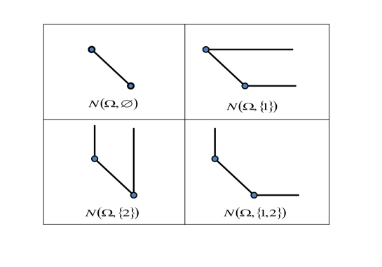
Figure 1. Newton Polyhedra ${\bf N}(\Omega,S)$ for $n=2$.

Definition 2.12.

Let $\Lambda=(\Lambda_{\nu})$ with $\Lambda_{\nu}\subset\mathbb{Z}_{+}^{n}$ and $S\subset\{1,\cdots,n\}$. Then, the ordered $d$-tuple of Newton polyhedra ${\bf N}(\Lambda_{\nu},S)$’s is defined by

$$\vec{{\bf N}}(\Lambda,S)=\left({\bf N}(\Lambda_{\nu},S)\right)_{\nu=1}^{d}.$$

To indicate a given polynomial $P=(P_{\nu})\in\mathcal{P}_{\Lambda}$, we also denote $\vec{{\bf N}}(\Lambda,S)$ by $\vec{{\bf N}}(P,S)$.

Definition 2.13.

Let $\Lambda=(\Lambda_{\nu})$ with $\Lambda_{\nu}\subset\mathbb{Z}_{+}^{n}$ and $S\subset\{1,\cdots,n\}$. We define the collection of $d$-tuples of faces $\mathbb{F}_{\nu}\in\mathcal{F}({\bf N}(\Lambda_{\nu},S))$ by

$$\mathcal{F}(\vec{{\bf N}}(\Lambda,S))=\{\mathbb{F}=\left(\mathbb{F}_{1},\cdots,\mathbb{F}_{d}\right):\mathbb{F}_{\nu}\in\mathcal{F}({\bf N}(\Lambda_{\nu},S))\}.$$

For each $\mathbb{F}\in\mathcal{F}(\vec{{\bf N}}(\Lambda,S))$, we denote $d$-tuple of cones by $\mathbb{F}^{*}=(\mathbb{F}_{\nu}^{*})$.

2.5. Basic Decompositions According to Faces and Cones

Choose $\,\psi\in C^{\infty}_{c}([-2,2])\,$ such that $\,0\leq\psi\leq 1\,$ and $\,\psi(u)=1\,$ for $\,|u|\leq 1/2\,.$ Put $\,\eta(u)=\psi(u)-\psi(2u)\,$ and $\,h(u)=\eta(u)/u\,$ for $\,u\neq 0\,.$ Let $\,\Lambda=\left(\Lambda_{1},\cdots,\Lambda_{d}\right)\,$ and $P_{\Lambda}\in\mathcal{P}_{\Lambda}$. For each $\mathbb{F}=(\mathbb{F}_{\nu})\in\mathcal{F}(\vec{{\bf N}}(\Lambda,S))$ and $\,J\in\mathbb{Z}^{n}\,,$ define

$$\mathcal{I}_{J}(P_{\mathbb{F}},\xi) = \int_{\mathbb{R}^{n}}\exp\left(i\,\sum_{\nu=1}^{d}\left(\sum_{\mathfrak{m}\in\mathbb{F}_{\nu}\cap\Lambda_{\nu}}c_{\mathfrak{m}}^{\nu}2^{-J\cdot\mathfrak{m}}t^{\mathfrak{m}}\right)\xi_{\nu}\right)\,\prod_{\ell=1}^{n}h(t_{\ell})\,dt$$

$$= \int_{\mathbb{R}^{n}}\exp\left(i\,\sum_{\mathfrak{m}\in\bigcup\mathbb{F}_{\nu}\cap\Lambda_{\nu}}2^{-J\cdot\mathfrak{m}}\langle\xi,c_{\mathfrak{m}}\rangle t^{\mathfrak{m}}\right)\,\prod_{\ell=1}^{n}h(t_{\ell})\,dt$$

where $c_{\mathfrak{m}}=(c^{\nu}_{\mathfrak{m}})$ defined in (1.1). We shall write $\mathcal{I}_{J}(P_{\Lambda},\xi)$ instead of $\mathcal{I}_{J}(P_{{\bf N}(\Lambda,S))},\xi)$.

Definition 2.14.

Given $S\subset N_{n}=\{1,\cdots,n\}$, we define

$$1_{S}=(r_{j})\ \text{where $r_{i}=1$ for $i\in S$ and $r_{i}=\infty$ for $i\in N_{n}\setminus S$}$$

and

$$Z(S)=\prod_{i=1}^{n}Z_{i}\ \ \text{where}\ \ Z_{i}=\mathbb{R}_{+}\ \ \text{if}\ \ i\in S\ \ \text{and}\ \ Z_{i}=\mathbb{R}\ \ \text{if}\ \ i\in N_{n}\setminus S.$$

Then by using $Z_{i}$ above, we write

$$\prod_{i\in S}\{-1<t_{i}<1\}\prod_{i\in N_{n}\setminus S}\{-\infty<t_{i}<\infty\}=\prod_{i=1}^{n}\left(\bigcup_{k_{i}\in Z_{i}\cap\,\mathbb{Z}}\{|t_{i}|\approx 2^{-k_{i}}\}\right),$$

and make the following dyadic decomposition:

(2.12) $$\mathcal{I}(P_{\Lambda},\xi,1_{S})=\sum_{J\in Z(S)\cap\mathbb{Z}^{n}}\mathcal{I}_{J}(P_{\Lambda},\xi).$$

As the name (dual face) tells, each $J\in\mathbb{F}^{*}_{\nu}\cap\mathbb{Z}^{n}$ can be understood as a linear functional mapping $\mathfrak{n}\in\mathbb{R}^{n}$ to $J\cdot\mathfrak{n}\in\mathbb{R}$ satisfying the following dominating property:

(2.13) $$2^{-J\cdot\mathfrak{m}}=2^{-r(J)}\geq 2^{-J\cdot\mathfrak{n}}\ \ \text{for all}\ \mathfrak{m}\in\mathbb{F}_{\nu}\ \text{and}\ \mathfrak{n}\in\mathbb{P}_{\nu}\setminus\mathbb{F}_{\nu}.$$

Thus, for $J\in\bigcap_{\nu=1}^{d}\mathbb{F}^{*}_{\nu}$ in (2.12) with the property (2.13) in (2.5),

(2.14) $$\exists\,\alpha\in\mathbb{Z}_{+}^{n}\,,\ \ \left(\frac{\partial}{\partial t}\right)^{\alpha}\left(\sum_{\nu=1}^{d}\left(\sum_{\mathfrak{m}\in\Lambda_{\nu}}c_{\mathfrak{m}}^{\nu}2^{-J\cdot\mathfrak{m}}t^{\mathfrak{m}}\right)\xi_{\nu}\right)\approx 2^{-J\cdot\mathfrak{m}_{\nu}}\xi_{\nu}\ \ \text{for all $\mathfrak{m}_{\nu}\in\mathbb{F}_{\nu}\cap\Lambda_{\nu}$}.$$

This combined with $Z(S)=\bigcup_{\mathbb{F}=(\mathbb{F}_{\nu})\in\mathcal{F}(\vec{{\bf N}}(\Lambda,S))}\left(\bigcap_{\nu=1}^{d}\mathbb{F}^{*}_{\nu}\right)$ suggests us to decompose in Section 6

$$\sum_{J\in Z(S)\cap\mathbb{Z}^{n}}\mathcal{I}_{J}(P_{\Lambda},\xi)=\sum_{\mathbb{F}\in\mathcal{F}(\vec{{\bf N}}(\Lambda,S))}\sum_{J\in\bigcap_{\nu=1}^{d}\mathbb{F}^{*}_{\nu}\cap\mathbb{Z}^{n}}\mathcal{I}_{J}(P_{\Lambda},\xi),$$

and next prove in Sections 7 and 8 that for each $\mathbb{F}=(\mathbb{F}_{\nu})\in\mathcal{F}(\vec{{\bf N}}(\Lambda,S))$,

(2.15) $$\qquad\sum_{s=1}^{N}\sum_{J\in\bigcap_{\nu=1}^{d}\mathbb{F}^{*}_{\nu}\cap\mathbb{Z}^{n}}\left|\mathcal{I}_{J}(P_{\mathbb{F}(s-1)},\xi)-\mathcal{I}_{J}(P_{\mathbb{F}(s)},\xi)\right|+\sum_{J\in\bigcap_{\nu=1}^{d}\mathbb{F}^{*}_{\nu}\cap\mathbb{Z}^{n}}\left|\mathcal{I}_{J}(P_{\mathbb{F}},\xi)\right|\leq C.$$

Here $\mathbb{F}(s)=(\mathbb{F}_{\nu}(s))$ will be chosen in an suitable way so that $\mathbb{F}_{\nu}(s-1)\succeq\mathbb{F}_{\nu}(s)$ with $\nu=1,\cdots,d$ where $\vec{{\bf N}}(\Lambda,S)=\mathbb{F}(0)$ and $\mathbb{F}(N)=\mathbb{F}$ as in (1).

3. Main Theorem and Background

In order to state main results, we first try to find an appropriate condition on an exponent set $\bigcup_{\nu=1}^{d}\mathbb{F}_{\nu}\cap\Lambda_{\nu}$ which guarantees $\mathcal{I}_{J}(P_{\mathbb{F}},\xi)\equiv 0$.

3.1. Even Sets

Let $\bigcup_{\nu=1}^{d}\mathbb{F}_{\nu}\cap\Lambda_{\nu}=\left\{\mathfrak{m}_{1},\cdots,\mathfrak{m}_{N}\right\}.$ Suppose every vector $\mathfrak{m}$ of the form

$$\alpha_{1}\mathfrak{m}_{1}+\cdots+\alpha_{N}\mathfrak{m}_{N}\ \text{with}\ \alpha_{j}=0\ \text{or}\ \ 1$$

has at least one even component. Then, the Taylor expansion of the exponential function in (2.5) yields that

(3.1) $$\mathcal{I}_{J}(\mathbb{F},\xi) = \sum_{k=0}^{\infty}\int_{\mathbb{R}^{n}}\,\frac{\left(i\sum_{\mathfrak{m}\in\bigcup\mathbb{F}_{\nu}\cap\Lambda_{\nu}}2^{-J\cdot\mathfrak{m}}\langle\xi,c_{\mathfrak{m}}\rangle t^{\mathfrak{m}}\right)^{k}}{k!}\,\prod_{\ell=1}^{n}h(t_{\ell})dt\,$$

$$= \sum_{k=0}^{\infty}\int_{\mathbb{R}^{n}}\,\sum_{\alpha_{1}+\cdots+\alpha_{N}=k}C(J,\mathfrak{m},\alpha,\xi)\frac{t^{\alpha_{1}\mathfrak{m}_{1}+\cdots+\alpha_{1}\mathfrak{m}_{N}}}{k!}\,\prod_{\ell=1}^{n}h(t_{\ell})dt=0$$

since $h(t_{\ell})$ is an odd function for each $\ell=1,\cdots,n$. This observation leads to the following notions of even and odd sets in $\mathbb{Z}_{+}^{n}$. Let $\Omega=\{\,\mathfrak{m}_{1},\cdots,\mathfrak{m}_{N}\,\}\subset\mathbb{Z}^{n}_{+}$ and let the class of sum of vectors in $\Omega$ be

$$\Sigma(\Omega)=\left\{\alpha_{1}\mathfrak{m}_{1}+\cdots+\alpha_{N}\mathfrak{m}_{N}:\alpha_{j}=0\ \text{or}\ \ 1\right\}.$$

Definition 3.1.

A finite subset $\Omega=\{\,\mathfrak{m}_{1},\cdots,\mathfrak{m}_{N}\,\}$ of $\mathbb{Z}_{+}^{n}$ is said to be odd iff there exists at least one vector $\mathfrak{m}\in\Sigma(\Omega)$ all of whose components are odd numbers such that

$$\mathfrak{m}=(\mbox{odd},\cdots,\mbox{odd}).$$

Definition 3.2.

A finite subset $\Omega$ of $\mathbb{Z}_{+}^{n}$ is said to be even iff $\Omega$ is not odd, that is, every $\mathfrak{m}=(m_{1},\cdots,m_{n})\in\Sigma(\Omega)$ has at least one even numbered component $m_{j}$.

Example 3.1.

In $\mathbb{Z}_{+}^{3}$, let $A=\{(1,1,0),(3,2,1)\}$, and $B=\{(1,1,0),(0,0,3)\}$. Then $A$ is an even set and $B$ an odd set. Notice that $A$ is an even set, though there is no $k\in\{1,2,3\}$ such that $k^{th}$ component of every vector in $A$ is even.

In (3.1), we have proved the following proposition:

Proposition 3.1.

Suppose that $\bigcup_{\nu=1}^{d}(\mathbb{F}_{\nu}\cap\Lambda_{\nu})$ is an even set. Then $\mathcal{I}_{J}(\mathbb{F},\xi)\equiv 0$

We shall perform the estimates (2.15) by using a full rank condition of $\bigcup\mathbb{F}_{\nu}(s)$ (formulated in Proposition 5.1) or vanishing property in Propositions 3.1. Thus, the evenness condition in Propositions 3.1 shall be imposed on the only faces contained in the subclass $\mathcal{A}$ of $\mathcal{F}(\vec{{\bf N}}(\Lambda,S))$ satisfying the following two conditions:

(3.2) Low Rank Condition:   $$\text{rank}\left(\bigcup_{\nu=1}^{d}\mathbb{F}_{\nu}\right)\leq n-1 \mathbb{F}\in\mathcal{A}$$ for ,

(3.3) Overlapping Cone Condition:   $$\bigcap_{\nu=1}^{d}(\mathbb{F}_{\nu}^{*})^{\circ}\neq\emptyset\ \mathbb{F}\in\mathcal{A}$$ for

where the overlapping cone condition comes from the decompositions in $J$ and the dominating condition (2.13).

3.2. Statement of Main Results

We start with the simplest case $d=1$. Observe for this case that $\bigcap_{\nu=1}^{d}\left(\mathbb{F}^{*}_{\nu}\right)^{\circ}\neq\emptyset$ always holds whenever $\text{rank}\left(\bigcup_{\nu=1}^{d}\mathbb{F}_{\nu}\right)\leq n-1.$

Main Theorem 1.

Let $\Lambda\subset\mathbb{Z}_{+}^{n}$ and $S\subset N_{n}$. Suppose that $d=1$ in (1.1). Let $1<p<\infty$. Then

$$\text{for all $P\in\mathcal{P}_{\Lambda}$,}\ \ \exists\,C_{P}>0\ \text{such that}\ \sup_{r\in I(S)}\left\|\mathcal{H}^{P}_{r}\right\|_{L^{p}(\mathbb{R}^{1})\rightarrow L^{p}(\mathbb{R}^{1})}\leq C_{P}$$

if and only if $\mathbb{F}\cap\Lambda$ is an even set for $\mathbb{F}\in\mathcal{F}({\bf N}(\Lambda,S))$ whenever $\text{rank}\left(\mathbb{F}\right)\leq n-1$.

For $d>1$, the overlapping condition (3.3) is crucial as well as the rank condition (3.2).

Definition 3.3.

Given $\vec{{\bf N}}(\Lambda,S)=\left({\bf N}(\Lambda_{\nu},S)\right)_{\nu=1}^{d}$, we set the collection of all $d$-tuples of faces satisfying both low rank condition (3.2) and overlapping (3.3) by

$$\mathcal{F}_{\rm{lo}}(\vec{{\bf N}}(\Lambda,S))=\left\{(\mathbb{F}_{\nu})\in\mathcal{F}\left(\vec{{\bf N}}(\Lambda,S)\right):\text{rank}\left(\bigcup_{\nu=1}^{d}\mathbb{F}_{\nu}\right)\leq n-1\ \text{and}\ \bigcap_{\nu=1}^{d}\left(\mathbb{F}^{*}_{\nu}\right)^{\circ}\neq\emptyset\right\}.$$

We assume first that $\Lambda_{\nu}$’s are mutually disjoint such that $\Lambda_{\mu}\cap\Lambda_{\nu}=\emptyset$ for any $\mu\neq\nu$.

Main Theorem 2.

Let $\Lambda=(\Lambda_{1},\cdots,\Lambda_{d})$ with $\Lambda_{\nu}\subset\mathbb{Z}_{+}^{n}$ and $S\subset N_{n}$. Suppose that $\Lambda_{\nu}$’s are mutually disjoint. Let $1<p<\infty$. Then

$$\text{for all $P\in\mathcal{P}_{\Lambda}$,}\ \ \exists\,C_{P}>0\ \text{such that}\ \sup_{r\in I(S)}\left\|\mathcal{H}^{P}_{r}\right\|_{L^{p}(\mathbb{R}^{d})\rightarrow L^{p}(\mathbb{R}^{d})}\leq C_{P}$$

if and only if  $\bigcup_{\nu=1}^{d}(\mathbb{F}_{\nu}\cap\Lambda_{\nu})$ is an even set for $\mathbb{F}=(\mathbb{F}_{\nu})\in\mathcal{F}_{\rm{lo}}(\vec{{\bf N}}(\Lambda,S))$.

Remark 3.1.

Main Theorems 1 and 2 do not give a criteria for the boundedness with a given individual polynomial $P_{\Lambda}$, but enables us to determine the boundedness for universal polynomials $P_{\Lambda}$ with a set $\Lambda$ of exponents fixed. Also, Main Theorems 1 and 2 do not give a condition for the boundedness of $\left\|\mathcal{H}^{P}_{r}\right\|_{L^{p}(\mathbb{R}^{d})\rightarrow L^{p}(\mathbb{R}^{d})}$ with fixed $r$, but for the uniform boundedness $\sup_{r\in I(S)}\left\|\mathcal{H}^{P}_{r}\right\|_{L^{p}(\mathbb{R}^{d})\rightarrow L^{p}(\mathbb{R}^{d})}$. It is interesting to know if $\sup_{r\in I(S)}\left\|\mathcal{H}^{P}_{r}\right\|_{L^{p}(\mathbb{R}^{d})\rightarrow L^{p}(\mathbb{R}^{d})}$ can be replaced by $\left\|\mathcal{H}^{P}_{1_{S}}\right\|_{L^{p}(\mathbb{R}^{d})\rightarrow L^{p}(\mathbb{R}^{d})}$ in the above theorems where $1_{S}$ is defined in Definition 2.14.

Let $P_{\Lambda}$ be a form of graph $(t_{1},\cdots,t_{n},P_{n+1}(t))$ so that $\Lambda=(\{{\bf e}_{1}\},\cdots,\{{\bf e}_{n}\},\Lambda_{n+1})$. For this case, we are able to show that the $L^{p}$ boundedness of $\mathcal{H}^{P_{\Lambda}}_{1_{S}}$ and the uniform $L^{p}$ boundedness of $\mathcal{H}^{P_{\Lambda}}_{r}$ in $r\in I(S)$ are equivalent. Moreover, we do not need the overlapping condition (3.3), since we can make the condition $\bigcap_{\nu=1}^{d}\left(\mathbb{F}^{*}_{\nu}\right)^{\circ}\neq\emptyset$ always hold.

Corollary 3.1.

Let $1<p<\infty$ and let $\Lambda=(\{{\bf e}_{1}\},\cdots,\{{\bf e}_{n}\},\Lambda_{n+1})$ and $S\subset N_{n}$. Then

$$\text{for all $P\in\mathcal{P}_{\Lambda}$,}\ \ \exists\,C_{P}>0\ \text{such that}\ \ \left\|\mathcal{H}^{P}_{1_{S}}\right\|_{L^{p}(\mathbb{R}^{d})\rightarrow L^{p}(\mathbb{R}^{d})}\leq C_{P}$$

if and only if $(\mathbb{F}_{n+1}\cap\Lambda_{n+1})\cup A$, for $\mathbb{F}_{n+1}\in\mathcal{F}({\bf N}(\Lambda_{n+1},S))$ and $A\subset\{{\bf e}_{1},\cdots,{\bf e}_{n}\}$, is an even set whenever $\text{rank}\left(\mathbb{F}_{n+1}\cup A\right)\leq n-1$.

Remark 3.2.

The above evenness condition in Corollary 3.1 is equivalent to

$$\bigcup_{\nu=1}^{d}(\mathbb{F}_{\nu}\cap\Lambda_{\nu})\ \text{ is an even set whenever $\text{rank}\left(\bigcup_{\nu=1}^{d}\mathbb{F}_{\nu}\right)\leq n-1$ for $\mathbb{F}\in\mathcal{F}(\vec{{\bf N}}(\Lambda,S))$.}$$

We exclude the assumption of mutually disjointness of $\Lambda_{\nu}$’s in the hypotheses of Main Theorem 2. Let $P=(P_{\nu})_{\nu=1}^{d}$ be a vector polynomial. For each $\nu=1,\cdots,d$, we define a set $\Lambda(P_{\nu})$ to be a set of all exponents of the monomials in $P_{\nu}$:

$$\Lambda(P_{\nu})=\left\{\mathfrak{m}\in\mathbb{Z}^{n}_{+}:c^{\nu}_{\mathfrak{m}}\neq 0\ \text{in $P_{\nu}(t)=\sum c^{\nu}_{\mathfrak{m}}t^{\mathfrak{m}}$}\right\}.$$

Moreover, we denote a $d$-tuple $(\Lambda(P_{\nu}))_{\nu=1}^{d}$ by $\Lambda(P)$. Denote the set of $d\times d$ invertible matrices by $GL(d)$. For $A\in GL(d)$ and $P\in\mathcal{P}_{\Lambda}$ with $P(t)=(P_{1}(t),\cdots,P_{d}(t))$, we let $AP$ be a vector polynomial given by the matrix multiplication

$$AP(t)=\left(\sum_{\mathfrak{m}\in\Lambda((AP)_{\nu})}a^{\nu}_{\mathfrak{m}}t^{\mathfrak{m}}\right)_{\nu=1}^{d}\ \ \text{for some $a_{\mathfrak{m}}^{\nu}\neq 0$}$$

where we regard $P(t)$ and $AP(t)$ above as column vectors. Then $AP\in\mathcal{P}_{\Lambda^{\prime}}$ where $\Lambda^{\prime}=\Lambda(AP)$. If $A=I$ an identity matrix, $\Lambda^{\prime}=\left(\Lambda((AP)_{\nu})\right)_{\nu=1}^{d}=\left(\Lambda(P_{\nu})\right)_{\nu=1}^{d}=(\Lambda_{\nu})_{\nu=1}^{d}=\Lambda$.

Definition 3.4.

Let $P\in\mathcal{P}_{\Lambda}$ where $\Lambda=(\Lambda_{\nu})$ with $\Lambda_{\nu}\subset\mathbb{Z}_{+}^{n}$ and $S\subset\{1,\cdots,n\}$. Let $A\in GL(d)$. Given a vector polynomial $AP$, we consider the $d$-tuple of Newton polyhedrons

$$\vec{{\bf N}}(AP,S)=\left({\bf N}((AP)_{\nu},S)\right)_{\nu=1}^{d}$$

and $d$-tuple of their faces

$$\mathcal{F}(\vec{{\bf N}}(AP,S))=\left\{\mathbb{F}_{A}=((\mathbb{F}_{A})_{1},\cdots,(\mathbb{F}_{A})_{d}):(\mathbb{F}_{A})_{\nu}\in\mathcal{F}\left({\bf N}((AP)_{\nu},S)\right)\right\}.$$

Main Theorem 3.

Let $\Lambda=(\Lambda_{1},\cdots,\Lambda_{d})$ with $\Lambda_{\nu}\subset\mathbb{Z}_{+}^{n}$ and $S\subset N_{n}$. Let $1<p<\infty$.

$$\text{For all $P\in\mathcal{P}_{\Lambda}$}\ \ \exists\ C_{P}>0\ \text{such that}\ \sup_{r\in I(S)}\left\|\mathcal{H}^{P}_{r}\right\|_{L^{p}(\mathbb{R}^{d})\rightarrow L^{p}(\mathbb{R}^{d})}\leq C_{P}\ \$$

if and only if for all $A\in GL_{d}$ and $P\in\mathcal{P}_{\Lambda},$

(3.4) $$\qquad\bigcup_{\nu=1}^{d}(\mathbb{F}_{A})_{\nu}\cap\Lambda((AP)_{\nu})\ \text{ is an even set whenever $\mathbb{F}_{A}=((\mathbb{F}_{A})_{\nu})\in\mathcal{F}_{\rm{lo}}(\vec{{\bf N}}(AP,S))$ }$$

where the class $\mathcal{F}_{\rm{lo}}(\vec{{\bf N}}(AP,S))$ is defined as in Definition 3.3.

Remark 3.3.

For the case $n=2$ in Main Theorems 2 and 3, the overlapping condition of cones in $\mathcal{F}_{\rm{lo}}(\vec{{\bf N}}(\Lambda,S))$ does not have to appear explicitly. By omitting the overlapping cone condition in $\mathcal{F}_{\rm{lo}}(\vec{{\bf N}}(\Lambda,S))$, we let

$$\mathcal{F}_{\rm{l}}(\vec{{\bf N}}(\Lambda,S))=\left\{(\mathbb{F}_{\nu})\in\mathcal{F}\left(\vec{{\bf N}}(\Lambda,S)\right):\text{rank}\left(\bigcup_{\nu=1}^{d}\mathbb{F}_{\nu}\right)\leq n-1\right\}\supset\mathcal{F}_{\rm{lo}}(\vec{{\bf N}}(\Lambda,S)).$$

Then, for the case $n=2$, the evenness condition for $\mathcal{F}_{\rm{lo}}(\vec{{\bf N}}(\Lambda,S))$ is equivalent to the condition for $\mathcal{F}_{\rm{l}}(\vec{{\bf N}}(\Lambda,S))$. It suffices to show $\Rightarrow$. Suppose that $\bigcup_{\nu=1}^{d}\mathbb{F}_{\nu}\cap\Lambda_{\nu}$ is an odd set with $\text{rank}\left(\bigcup_{\nu=1}^{d}\mathbb{F}_{\nu}\right)\leq 1$. Then there exists $\mu$ such that $\mathbb{F}_{\mu}\cap\Lambda_{\mu}$ has a point $(odd,odd)$, because both of two points $(even,odd),(odd,even)$ can not lie in the one line passing through the origin. Therefore, $\mathbb{G}=(\mathbb{G}_{\nu})$ defined by $\mathbb{G}_{\mu}=\mathbb{F}_{\mu}$ and $\mathbb{G}_{\nu}=\emptyset$ for $\nu\neq\mu$ satisfies that $\mathbb{G}\in\mathcal{F}_{\rm{lo}}(\vec{{\bf N}}(\Lambda,S))$ and $\bigcup_{\nu=1}^{d}\mathbb{G}_{\nu}\cap\Lambda_{\nu}$ is an odd set.

Remark 3.4.

For the case $n\geq 3$, the overlapping condition is crucial in Main Theorems 2 and 3. Moreover, we note that it is not just cones $\bigcap_{\nu=1}^{d}\mathbb{F}_{\nu}^{*}$, but their interiors $\bigcap_{\nu=1}^{d}(\mathbb{F}_{\nu}^{*})^{\circ}$ that satisfy the overlapping condition (3.3). The example 4.1 in Section 4 shows that there exists $\mathbb{F}\in\mathcal{F}_{\rm{l}}(\vec{{\bf N}}(\Lambda,S))$ such that $\bigcap_{\nu=1}^{d}\mathbb{F}_{\nu}^{*}\neq\emptyset$ and $\bigcup_{\nu=1}^{d}(\mathbb{F}_{\nu}\cap\Lambda_{\nu})$ is an odd set, but

$$\text{ for all $P\in\mathcal{P}_{\Lambda}$ }\ \ \sup_{r\in I(S)}\left\|\mathcal{H}^{P}_{r}\right\|_{L^{p}(\mathbb{R}^{d})\rightarrow L^{p}(\mathbb{R}^{d})}\leq C_{P}.$$

3.3. Background

In the one parameter case ($n=1$), the operator $\mathcal{H}^{P_{\Lambda}}_{r}$ with $r=(1,\cdots,1)$ can be regarded as a particular instance of singular integrals along curves satisfying finite type condition in E. M. Stein and S. Wainger [21]. The $L^{p}$ theory of those singular integrals has been developed quite well. For example, see M. Christ, A. Nagel, E. M. Stein and S. Wainger [6] for singular Radon transforms with the curvature conditions in a very general setting. See also M. Folch-Gabayet and J. Wright [8] for the case that phase functions $P_{\Lambda}$ are given by rational functions.

In the multi-parameter case ($\,n\geq 2\,$), it is A. Nagel and S. Wainger [12] who introduced the (global) multiple Hilbert transforms along surfaces having certain dilation invariance properties and obtained their $L^{2}$ boundedness. In [17], F. Ricci and E. M. Stein established an $L^{p}$ theorem for multi-parameter singular integrals whose kernels satisfy more general dilation structure. A special case of their results implies that if $\Lambda=\left(\{{\bf e}_{1}\},\cdots,\{{\bf e}_{n}\},\{\mathfrak{m}\}\right)$ where at least $n-1$ coordinates of $\mathfrak{m}$ are even, then $\|\mathcal{H}^{P_{\Lambda}}_{1_{S}}\|_{L^{p}(\mathbb{R}^{n+1})\rightarrow L^{p}(\mathbb{R}^{n+1})}$ are bounded for $1<p<\infty$. In [3], A. Carbery, S. Wainger and J. Wright obtained a necessary and sufficient condition for $L^{p}(\mathbb{R}^{3})$ boundedness of $\mathcal{H}_{1_{S}}^{\Lambda}$ with $S=\{1,2\}$, $\Lambda=(\{{\bf e}_{1}\},\{{\bf e}_{2}\},\Lambda_{3})$ where $d=3$ and $n=2$. Their theorem states that

Theorem 3.1 (Double Hilbert transform [3]).

Let $\,\Lambda=\left(\{{\bf e}_{1}\},\{{\bf e}_{2}\},\Lambda_{3}\right)$ and $S=\{1,2\}$ with $n=2$ and $d=3$. For $1<p<\infty$, the local double Hilbert transform $\mathcal{H}^{P_{\Lambda}}_{1_{S}}$ is bounded in $L^{p}(\mathbb{R}^{3})$ if and only if every vertex $\mathfrak{m}$ in ${\bf N}(\Lambda_{3},S)$ has at least one even component.

S. Patel [14] extends this result to $S=\emptyset$ corresponding to the global Hilbert transform.

Theorem 3.2 (Double Hilbert transform [14]).

Let $\,\Lambda=\left(\{{\bf e}_{1}\},\{{\bf e}_{2}\},\Lambda_{3}\right)$ and $S=\{\emptyset\}$ with $n=2$ and $d=3$. For $1<p<\infty$, the global double Hilbert transform $\mathcal{H}^{P_{\Lambda}}_{1_{S}}$ is bounded in $L^{p}(\mathbb{R}^{3})$ if and only if every vertex $\mathfrak{m}$ in ${\bf Ch}(\Lambda_{3})$ and every edge $E$ in ${\bf Ch}(\Lambda_{3})$ passing through the origin has at least one even component.

S. Patel [13] also studies the case $n=2$ and $d=1$. He has shown that the necessary and sufficient condition for the $L^{p}$ boundedness of $\mathcal{H}^{P_{\Lambda}}_{1_{S}}$ cannot be determined by only the geometry of ${\bf N}(\Lambda)$ but by coefficients of the given polynomial $P_{\Lambda}(t)$. More precisely, the condition is described in terms of not a single vertex $\mathfrak{m}$ and its coefficient $c_{\mathfrak{m}}$ in $P_{\Lambda}$, but the sum of quantities associated with many vertices and their corresponding coefficients:

Theorem 3.3 (Double Hilbert transform [13]).

Let $\,\Lambda=\left(\Lambda_{1}\right)$ and $S=\{1,2\}$ with $n=2$ and $d=1$. Then, the local double Hilbert transform $\mathcal{H}^{P_{\Lambda}}_{1_{S}}$ is bounded in $L^{p}(\mathbb{R}^{1})$ for $1<p<\infty$ if and only if

(3.5) $$\sum_{(m_{j},n_{j})\in\mathcal{F}^{0}_{odd}}\frac{\text{sgn}(a_{m_{j}n_{j}})}{m_{j}n_{j}}\left(\begin{matrix}m_{j}&0\\ 0&n_{j}\end{matrix}\right)(\mathfrak{n}_{j}^{+}-\mathfrak{n}_{j}^{-})=0.$$

where $\mathcal{F}^{0}_{odd}=\left\{(m_{j},n_{j})\in\mathcal{F}^{0}({\bf N}(\Lambda)):(m_{j},n_{j})=(odd,odd)\right\}$, and $(m_{j},n_{j})\in\mathcal{F}^{0}_{odd}$ is an intersection $\mathbb{F}_{j}^{-}\cap\mathbb{F}_{j}^{+}$ of two facets $\mathbb{F}_{j}^{\pm}=\pi_{\mathfrak{n}^{\pm}_{j},1}\cap{\bf N}(\Lambda)\in\mathcal{F}^{1}({\bf N}(\Lambda))$.

A. Carbery, S. Wainger and J. Wright [2] obtain the asymptotic behaviors of the oscillatory singular integrals associated with analytic phase functions $P(t_{1},t_{2})$, which extends Theorem 3.1 to the class of analytic functions. They [2] also find an example of finite type surface $(t_{1},t_{2},P(t_{1},t_{2}))$ with its formal Taylor series satisfying evenness hypothesis, however $\mathcal{H}_{r}^{P}$ not bounded in $L^{2}(\mathbb{R}^{3})$. We also refer to [5] dealing with a certain class of flat surfaces $(t_{1},t_{2},P(t_{1},t_{2}))$ without any curvature. In the general setting of polynomial surfaces defining the Double Hilbert transform, M. Pramanik and C. W. Yang [16] obtain the $L^{p}$ theorem:

Theorem 3.4 (Double Hilbert transform [16]).

Let $\,\Lambda=\left(\{{\bf e}_{1}\},\{{\bf e}_{2}\},\Lambda_{1},\cdots,\Lambda_{k}\right)$ and $S=\{1,2\}$ with $n=2$ and $d=k+2$. Suppose that $P(t_{1},t_{2})=(P_{\Lambda_{1}}(t),\cdots,P_{\Lambda_{k}}(t))$ and $P_{\Lambda}=(t_{1},t_{2},P(t_{1},t_{2}))$. For $1<p<\infty$, the local double Hilbert transform $\mathcal{H}^{P_{\Lambda}}_{1_{S}}$ is bounded in $L^{p}(\mathbb{R}^{d})$ if and only if for every $A\in GL(k)$, every vertex $\mathfrak{m}\in{\bf N}((AP)_{\nu},S)$ with $\nu=1,\cdots,k$ has at least one even numbered component.

Remark 3.5.

The results of Main Theorems 2 and 3 for $n=2$ and $S=\{1,2\}$ follows from Theorem 3.4 by a slight modification of its necessary proof.

The triple Hilbert transforms $\mathcal{H}^{P_{\Lambda}}_{1_{S}}$ with $S=\{1,2,3\}$ and $\Lambda=(\{{\bf e}_{1}\},\{{\bf e}_{2}\},\{{\bf e}_{3}\},\Lambda_{4})$ were studied in the two papers [3] [4] published in 2009. In [3], A. Carbery, S. Wainger and J. Wright have discovered a remarkable differences between the triple and the double Hilbert transforms. The $L^{2}$ boundedness of the triple Hilbert transform $\mathcal{H}^{P_{\Lambda}}_{1_{S}}$ depends on the coefficients of $P_{\Lambda}$ as well as the Newton polyhedron ${\bf N}(\Lambda_{4})$, whereas that of the double Hilbert transform depends only on the Newton polygon ${\bf N}(\Lambda_{3})$. They establish two types of theorems. First one gives the necessary and sufficient condition that the operators $\mathcal{H}^{P_{\Lambda}}_{1_{S}}$ are bounded in $L^{2}$ for all class of polynomials $P_{\Lambda}\in\mathcal{P}(\Lambda)$ when $\Lambda$ is given. This theorem is called the universal theorem. The second theorem is to inform the necessary and sufficient condition that the one individual operator $\mathcal{H}^{P_{\Lambda}}_{1_{S}}$ is bounded in $L^{2}$ when a polynomial $P_{\Lambda}$ is given. This theorem is called the individual theorem. The condition of the first theorem is expressed solely in terms of ${\bf N}(\Lambda_{4})$ but that of the second in terms of individual coefficients of given polynomial $P_{\Lambda}$ in question. Here we only state their universal theorem.

Theorem 3.5 (Triple Hilbert transform [3]).

Let $\,1<p<\infty\,.$ Given $S=\{1,2,3\}$ and $\,\Lambda=\left(\{{\bf e}_{1}\},\{{\bf e}_{2}\},\{{\bf e}_{3}\},\Lambda_{4}\right)$, suppose that

• Every entry of a vertex in ${\bf N}(\Lambda_{4},S)$ is positive.

• • Each edge ${\bf N}(\Lambda_{4},S)$ is not contained on any hyperplane parallel to a coordinate plane.

  • The projection of the line containing an edge ${\bf N}(\Lambda_{4},S)$ onto a coordinate plane does not pass through the origin.

• The plane determined by any three vertices in ${\bf N}(\Lambda_{4},S)$ does not contain the origin.

Then the triple Hilbert transform $\mathcal{H}^{P_{\Lambda}}_{1_{S}}$ is bounded in $L^{2}(\mathbb{R}^{4})$ for all $P_{\Lambda}\in\mathcal{P}_{\Lambda}$ if and only if every vertex in ${\bf N}(\Lambda_{4},S)$ has at least two even entries, and every edges $E$ of ${\bf N}(\Lambda_{4},S)$ satisfies that there exists a one component such that the entry of that component of every vector in $E\cap\Lambda_{4}$ is even.

Remark 3.6.

They found a vector polynomial $P_{\Lambda}(t)=(t_{1},t_{2},t_{3},P_{\Lambda_{4}}(t))$ such that the corresponding triple Hilbert transform $\mathcal{H}^{P_{\Lambda}}_{1_{S}}$ is bounded on $L^{2}(\mathbb{R}^{4})$ although ${\bf N}(\Lambda_{4},S)$ breaks the above evenness condition.

In [4], Y.K. Cho, H. Hong, C.W. Yang and the author proved the theorem without assuming the three hypotheses H1-H3 so that

Theorem 3.6 (Triple Hilbert transform [4]).

Let $\,1<p<\infty\,.$ Given $S=\{1,2,3\}$ and $\,\Lambda=\left(\{{\bf e}_{1}\},\{{\bf e}_{2}\},\{{\bf e}_{3}\},\Lambda_{4}\right),$ the triple Hilbert transform $\mathcal{H}^{P_{\Lambda}}_{1_{S}}$ is bounded in $L^{p}(\mathbb{R}^{4})$ for all $P_{\Lambda}\in\mathcal{P}_{\Lambda}$ if and only if every $\mathbb{F}\in\mathcal{F}({\bf N}(\Lambda_{4}))$ for $\text{rank}\left((\mathbb{F}\cap\Lambda_{4})\cup A\right)\leq 2$ with $A\subset\{{\bf e}_{1},{\bf e}_{2},{\bf e}_{3}\}$ satisfies that there exists a one component such that the entry of that component of every vector in $\mathbb{F}\cap\Lambda_{4}$ is even.

Remark 3.7.

The hypotheses in Theorems 3.1, 3.2, 3.5 and 3.6 are same as those of Corollary 3.1 for $n=2,3$. It is interesting to find for $n\geq 3$ an asymptotic behavior of $\mathcal{I}(P_{\Lambda},\xi,1_{S})$ with a coefficient of logarithm in $\xi$ having a similar form to (3.5) in Theorem 3.3.

As a variable coefficient version, we define $\mathcal{H}^{P}(f)(x)$ by

$$\int_{\prod_{j=1}^{n}\,[-r_{j},r_{j}]}f\bigl{(}x_{1}-t_{1},\cdots,x_{n}-t_{n},x_{n+1}-P(x_{1},\cdots,x_{n},t_{1},\cdots,t_{n})\bigr{)}\,\frac{dt_{1}}{t_{1}}\cdots\frac{dt_{n}}{t_{n}}$$

whose corresponding oscillatory singular integral operator is given by

$$\mathcal{T}^{P}_{\lambda}\,(f)(x) = \text{p.v.}\int_{\{y:|x_{j}-y_{j}|<r_{j}\}}\frac{e^{i\lambda P(x,y)}}{(x_{1}-y_{1})\cdots(x_{n}-y_{n})}\,f(y)dy_{1}\cdots dy_{n}.$$

In view of the analogy between the integral operators of D. H. Phong and E. M. Stein [15] and the scalar valued integral of Varchenko [23], one may find the criteria for determining the uniform $L^{2}$ boundedness $\mathcal{T}^{P}_{\lambda}$ in $\lambda$ in terms of the Newton polyhedron associated with the polynomial $P(x,y)$. More generalized version is the multi-parameter singular Radon transform:

$$\mathcal{R}^{P_{\Lambda}}\,(f)(x) = \text{p.v.}\int_{\prod_{j=1}^{n}\,[-r_{j},r_{j}]}f\bigl{(}P_{\Lambda}(x,t)\bigr{)}\,\frac{dt_{1}}{t_{1}}\cdots\frac{dt_{n}}{t_{n}}.$$

Recently, E. M. Stein and B. Street in [22, 19, 20] obtain the $L^{p}$ boundedness for a certain class of multi-parameter singular Radon transform. A. Nagel, F. Ricci, E. M. Stein and S. Wainger in [10] study the singular integral operators on a homogeneous nilpotent Lie group that are given by convolution with flag kernels. Here flag kernels are product type singular kernels that are generalized version of our kernel $\frac{1}{t_{1}}\cdots\frac{1}{t_{n}}$. This result was preceded by [9] that proves the $L^{p}$ boundedness of convolution operators with some special type of flag kernels. This result applies to obtain $L^{p}$ regularity for the solutions of Cauchy-Riemann equations on CR manifolds.

4. Representation of faces and their cones

We study representations of faces $\mathbb{F}$ and their cones $\mathbb{F}^{*}$ of a polyhedron $\mathbb{P}=\mathbb{P}(\Pi)$ in $\mathbb{R}^{n}$. It is well known that every face $\mathbb{F}$ has an expression $\bigcap_{j=1}^{N}\pi_{\mathfrak{q}_{j},r_{j}}\cap\mathbb{P}$ with some generators $\pi_{\mathfrak{q}_{j},r_{j}}\in\Pi$ and its cone $\mathbb{F}^{*}$ expressed as $\text{CoSp}(\{\mathfrak{q}_{j}\}_{j=1}^{N})$. We shall prove this representation formula and give some detailed description of generators for the case $\text{dim}(\mathbb{P})<n$.

4.1. Low Dimensional Polyhedron in $\mathbb{R}^{n}$

A polyhedron $\mathbb{P}=\mathbb{P}(\Pi)$ in $\mathbb{R}^{n}$ with $\text{dim}(\mathbb{P})=m\leq n$ is regarded as a $m$ dimensional polyhedron in the affine space $V_{am}(\mathbb{P})$ of dimension $m$ defined in (2.1). Since $V_{am}(\mathbb{P})$ itself is a polyhedron in $\mathbb{R}^{n}$, we choose the generator $\Pi$ of $\mathbb{P}$ and split it into two parts $\Pi=\Pi_{a}\cup\Pi_{b}$: $\Pi_{b}$ a generator of $V_{am}(\mathbb{P})$ and $\Pi_{a}$ a generator of $\mathbb{P}$ in $V_{am}(\mathbb{P})$. See the left picture in Figure 2.

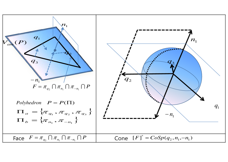
Figure 2. Low Dimensional Polyhedron, Face and Cone.

Lemma 4.1.

Let $\mathbb{P}\subset\mathbb{R}^{n}$ be a polyhedron with $\text{dim}(\mathbb{P})=\text{dim}(V_{am}(\mathbb{P}))=m\leq n$. Then $\mathbb{P}=\mathbb{P}(\Pi_{a}\cup\Pi_{b})$ such that

(4.1) $$\qquad V_{am}(\mathbb{P}) = \mathbb{P}(\Pi_{b})\ \text{in $\mathbb{R}^{n}$ with}\ \Pi_{b}=\{\pi_{\pm\mathfrak{n}_{i},\pm s_{i}}\}_{i=1}^{n-m}\ \text{with}\ \mathfrak{n}_{i}\perp\mathfrak{n}_{j}\ \text{for}\ i\neq j\,,$$

(4.2) $$\mathbb{P} = \mathbb{P}(\Pi_{a}^{\prime})\ \text{in $V_{am}(\mathbb{P})$ with}\ \Pi_{a}=\{\pi_{\mathfrak{q}_{j},r_{j}}\}_{j=1}^{M}\ \text{and}\ \Pi_{a}^{\prime}=\{\pi_{\mathfrak{q}_{j},r_{j}}\cap V_{am}(\mathbb{P})\}_{j=1}^{M},$$

where $\mathfrak{q}_{j}\in V(\mathbb{P})=\text{Sp}^{\perp}(\{\mathfrak{n}_{i}\}_{i=1}^{n-m})$.

Proof.

If $n=m$, then let $\Pi_{a}=\Pi$ and $\Pi_{b}=\emptyset$ so that $\mathbb{P}(\Pi_{b})=\mathbb{R}^{n}$. Let $m<n$. There exist $n-m$ orthonormal vectors $\mathfrak{n}_{j}$’s and some constants $s_{j}$’s such that

$$V(\mathbb{P})=\bigcap_{i=1}^{n-m}\pi_{\mathfrak{n}_{i},0}\ \ \text{so that}\ \ V_{am}(\mathbb{P})=\bigcap_{i=1}^{n-m}\pi_{\mathfrak{n}_{i},s_{i}}.$$

where $V(\mathbb{P})=\text{Sp}^{\perp}(\{\mathfrak{n}_{i}\}_{i=1}^{n-m})$. By (2.1), $V_{am}(\mathbb{P})=V(\mathbb{P})+\mathfrak{r}$ with $\mathfrak{r}\in\mathbb{P}$ and $s_{i}=\mathfrak{r}\cdot\mathfrak{n}_{i}$. This combined with $\pi_{\mathfrak{n}_{i},s_{i}}^{+}\cap\pi_{-\mathfrak{n}_{i},-s_{i}}^{+}=\pi_{\mathfrak{n}_{i},s_{i}}$ implies

$$V_{am}(\mathbb{P})=\mathbb{P}(\Pi^{b})\ \ \text{with}\ \ \Pi_{b}=\{\pi_{\pm\mathfrak{n}_{i},\pm s_{i}}:i=1,\cdots,n-m\},$$

which yields (4.1). By Definition 2.3, there are $\mathfrak{p}_{j}\in\mathbb{R}^{n}$ such that

(4.3) $$\mathbb{P}=\bigcap_{j}\{{\bf x}\in V_{am}(\mathbb{P}):\langle\mathfrak{p}_{j},{\bf x}\rangle\geq\rho_{j}\}.$$

Let ${\bf x}\in\mathbb{P}$ and $P_{V(\mathbb{P})}$ be a projection map to the vector space $V(\mathbb{P})$. Then from ${\bf x}-\mathfrak{r}\in V(\mathbb{P})$,

$$\langle\mathfrak{p}_{j},{\bf x}\rangle=\langle P_{V(\mathbb{P})}(\mathfrak{p}_{j}),{\bf x}\rangle+\langle P_{V^{\perp}(\mathbb{P})}(\mathfrak{p}_{j}),{\bf x}\rangle=\langle P_{V(\mathbb{P})}(\mathfrak{p}_{j}),{\bf x}\rangle+\langle Proj_{V^{\perp}(\mathbb{P})}(\mathfrak{p}_{j}),{\bf\mathfrak{r}}\rangle.$$

We put $Proj_{V(\mathbb{P})}(\mathfrak{p}_{j})=\mathfrak{q}_{j}$ and $r_{j}=\rho_{j}-\langle Proj_{V^{\perp}(\mathbb{P})}(\mathfrak{p}_{j}),\mathfrak{r}\rangle$ and rewrite (4.3) as

$$\mathbb{P}=\bigcap_{j=1}^{M}\{{\bf x}\in V_{am}(\mathbb{P}):\langle\mathfrak{q}_{j},{\bf x}\rangle\geq r_{j}\}\ \text{where}\ \mathfrak{q}_{j}=Proj_{V(\mathbb{P})}(\mathfrak{p}_{j})\in V(\mathbb{P})=\text{Sp}^{\perp}(\{\mathfrak{n}_{i}\}_{i=1}^{n-m}).$$

This proves (4.2). Finally, $\mathbb{P}=\mathbb{P}(\Pi_{a}\cup\Pi_{b})$ follows from (4.1) and (4.2). ∎

4.2. Representation of Face

Lemma 4.2.

Let $\mathbb{P}=\mathbb{P}(\Pi)$ with $\text{dim}(V_{am}(\mathbb{P}))=m$ and $\mathbb{F}$ be a proper face of $\mathbb{P}$. Then

$$\exists\,\pi\in\Pi\ \ \text{such that}\ \ \mathbb{F}\subset\pi.$$

Proof.

By Definition 2.8 and by Lemma 2.2,

(4.4) $$\mathbb{F}\subset\partial\mathbb{P}\subset\bigcup_{\pi\in\Pi}\pi\cap\mathbb{P}.$$

By (4.2) of Lemma 4.1, we may take $\Pi=\Pi_{a}^{\prime}$ in (4.4). Thus from (2) of Lemma 2.1, each $\pi\cap\mathbb{P}$ with $\pi\in\Pi$ is a face of $\mathbb{P}$ with dimension $m-1$. Therefore the second $\subset$ in (4.4) is replaced by $=$. We next use the same argument as in the proof of Lemma 2.3 to obtain that $\mathbb{F}$ in (4.4) is contained in one face $\pi\cap\mathbb{P}$ in (4.4). ∎

Definition 4.1 (Facet).

Let $\mathbb{P}=\mathbb{P}(\Pi)$ be a polyhedron in an affine space $V$ such that $\text{dim}(\mathbb{P})=\text{dim}(V_{am}(\mathbb{P}))=m$. Then $m-1$ dimensional face $\mathbb{F}$ of $\mathbb{P}$ is called a facet of $\mathbb{P}$.

Lemma 4.3.

Let $\mathbb{P}=\mathbb{P}(\Pi)$ be a polyhedron in an affine space $V$ such that $\text{dim}(\mathbb{P})=\text{dim}(V_{am}(\mathbb{P}))=m$ where $\Pi=\Pi_{a}\cup\Pi_{b}$ as in Lemma 4.1. Then every facet $\mathbb{F}$ of $\mathbb{P}$ is expressed as

$$\mathbb{F}=\pi\cap\mathbb{P}\ \ \text{and}\ \ \mathbb{P}\setminus\mathbb{F}\subset(\pi^{+})^{\circ}\ \text{for some $\pi\in\Pi_{a}\subset\Pi$}.$$

Proof.

By Lemma 4.1, we regard $\mathbb{P}=\mathbb{P}(\Pi^{\prime}_{a})$ as a polyhedron in the $m$ dimensional affine space $V_{am}(\mathbb{P})$. Here $\pi^{\prime}=\pi\cap V_{am}(\mathbb{P})\in\Pi_{a}^{\prime}$ is a $m-1$ dimensional hyperplane in $V_{am}(\mathbb{P})$. By Lemma 4.2,

(4.5) $$\exists\,\pi^{\prime}\in\Pi^{\prime}_{a}\ \ \text{such that}\ \ \mathbb{F}\subset\pi^{\prime}=\pi\cap V_{am}(\mathbb{P})\ \ \text{where}\ \pi\in\Pi_{a}.$$

On the other hand, by Definition 2.7, there exists an $m-1$ dimensional hyperplane $\pi_{\mathfrak{q},r}$ in $V_{am}(\mathbb{P})$ such that

(4.6) $$\mathbb{F}=\pi_{\mathfrak{q},r}\cap\mathbb{P} \mathbb{P}\setminus\mathbb{F}\subset(\pi_{\mathfrak{q},r}^{+})^{\circ}$$ and .

In view of (4.5) and (4.6), both $m-1$ dimensional hyperplanes $\pi^{\prime}$ and $\pi_{\mathfrak{q},r}$ in $V_{am}(\mathbb{P})$ contain the $m-1$ dimensional polyhedron $\mathbb{F}$. Thus $\pi^{\prime}=\pi_{\mathfrak{q},r}$. By this and (4.6),

$$\mathbb{F}=\pi_{\mathfrak{q},r}\cap\mathbb{P}=\pi^{\prime}\cap\mathbb{P}=\left(\pi\cap V_{am}(\mathbb{P})\right)\cap\mathbb{P}=\pi\cap\mathbb{P}\ \text{where $\pi\in\Pi_{a}$}$$

and $\mathbb{P}\setminus\mathbb{F}\subset(\pi_{\mathfrak{q},r}^{+})^{\circ}=((\pi^{\prime})^{+})^{\circ}\subset(\pi^{+})^{\circ}.$ ∎

Proposition 4.1 (Face Representation).

Let $\mathbb{P}=\mathbb{P}(\Pi)$ be a polyhedron in $\mathbb{R}^{n}$ where $\Pi=\Pi_{a}\cup\Pi_{b}$ as in Lemma 4.1. Let $\text{dim}(\mathbb{P})=m\leq n.$ Then every face $\mathbb{F}$ of $\mathbb{P}$ with $\text{dim}(\mathbb{F})\leq n-1$ has the expression

(4.7) $$\mathbb{F}=\bigcap_{\pi\in\Pi(\mathbb{F})}\mathbb{F}_{\pi}\ \ \text{where $\mathbb{F}_{\pi}=\pi\cap\mathbb{P}$ }\ \text{where}\ \ \Pi(\mathbb{F})=\{\pi_{\mathfrak{p}_{j}}\}_{j=1}^{N}\subset\Pi.$$

Remark 4.1.

We split the generator $\Pi(\mathbb{F})=\{\pi_{\mathfrak{p}_{j}}\}_{j=1}^{N}=\Pi_{a}(\mathbb{F})\cup\Pi_{b}(\mathbb{F})$ in (4.7) so that

(4.8) $$\quad\Pi_{a}(\mathbb{F})=\Pi(\mathbb{F})\cap\Pi_{a}=\{\pi_{\mathfrak{q}_{j}}\}_{j=1}^{\ell}\ \ \text{and}\ \ \Pi_{b}(\mathbb{F})=\Pi(\mathbb{F})\cap\Pi_{b}=\Pi_{b}=\{\pi_{\pm\mathfrak{n}_{i}}\}_{i=1}^{n-m}.$$

See the left side of Figure 2. Denote only normal vectors $\{\mathfrak{p}_{j}\}_{j=1}^{N}$ in $\Pi(\mathbb{F})$ by $\Pi(\mathbb{F})$ also.

Proof of Proposition 4.1.

Let $\text{dim}(\mathbb{F})=m\leq n-1$. An improper face $\mathbb{F}=\mathbb{P}$ has an expression

$$\mathbb{P}=\bigcap_{\pi\in\Pi_{b}}\pi\cap\mathbb{P}\ \ \text{where\ $\pi\in\Pi_{b}$}.$$

It suffices to show that each proper face $\mathbb{F}$ of $\mathbb{P}(\Pi)$ is expressed as

(4.9) $$\mathbb{F}=\bigcap_{j=1}^{M}\mathbb{F}_{j}\ \ \text{ where $\mathbb{F}_{j}=\pi_{j}\cap\mathbb{P}$ with $\pi_{j}\in\Pi_{a}\subset\Pi$ are facets of $\mathbb{P}$}.$$

To show (4.9), we first let $\mathbb{F}$ be a face of codimension 1 of the $m$-dimensional ambient affine space $V_{am}(\mathbb{P})$. Then $\mathbb{F}$ itself is a facet of $\mathbb{P}$ such that $\mathbb{F}=\pi\cap\mathbb{P}$ with $\pi\in\Pi_{a}\subset\Pi$ from Lemma 4.3. Let $\mathbb{F}$ be a face of codimension 2 of the $m$-dimensional ambient affine space $V_{am}(\mathbb{P})$. By Lemma 4.2,

$$\pi_{\mathfrak{q},r}\in\Pi_{a} \mathbb{F}\subset\pi_{\mathfrak{q},r}$$ such that .

By (2) of Lemma 2.1,

(4.10) $$\mathbb{P}^{\prime}=\pi_{\mathfrak{q},r}\cap\mathbb{P} \mathbb{P} \text{dim}(\mathbb{P}^{\prime})=m-1$$ is a facet of such that .

Moreover, observe that $\mathbb{P}^{\prime}$ itself is an $m-1$ dimensional polyhedron with

(4.11) $$\Pi_{a}(\mathbb{P}^{\prime})\subset\{\pi_{\mathfrak{q},r}\cap\pi:\pi\in\Pi_{a}(\mathbb{P})\}.$$

By $\mathbb{F}\subset\mathbb{P}^{\prime}$ and (1) of Lemma 2.1, $m-2$ dimensional face $\mathbb{F}$ of $\mathbb{P}$ is a facet of an $m-1$ dimensional polyhedron $\mathbb{P}^{\prime}$. Hence by Lemma 4.3, there exists $\pi^{\prime}\in\Pi_{a}(\mathbb{P}^{\prime})$ in (4.11) such that $\mathbb{F}=\pi^{\prime}\cap\mathbb{P}^{\prime}$. Thus, by (4.11) there exists $\pi\in\Pi_{a}(\mathbb{P})$ such that $\pi^{\prime}=\pi_{\mathfrak{q},r}\cap\pi$ and

$$\mathbb{F}=\pi^{\prime}\cap\mathbb{P}^{\prime}=(\pi_{\mathfrak{q},r}\cap\pi)\cap\mathbb{P}^{\prime}=\left(\pi_{\mathfrak{q},r}\cap\mathbb{P}\right)\cap\left(\pi\cap\mathbb{P}\right)=\mathbb{F}_{\pi_{\mathfrak{q},r}}\cap\mathbb{F}_{\pi}$$

where $\mathbb{F}_{\pi}$ and $\mathbb{F}_{\pi_{\mathfrak{q},r}}$ are facets of $\mathbb{P}$. We finish the proof of (4.9) inductively. ∎

4.3. Representation of Cone

Proposition 4.2 (Cone representation).

Every proper face $\mathbb{F}\preceq\mathbb{P}=\mathbb{P}(\Pi)$ having a generator $\Pi(\mathbb{F})=\{\mathfrak{p}_{j}\}_{j=1}^{N}$ with expression (4.7) has its cone of the form:

$$(\mathbb{F}^{*})^{\circ}|\mathbb{P} = (\mathbb{F}^{*})^{\circ}|(\mathbb{P},\mathbb{R}^{n})=\rm{CoSp}^{\circ}(\{\mathfrak{p}_{i}:i=1,\cdots,N\}).$$

Here $\mathbb{F}^{*}|\mathbb{P}=\mathbb{F}^{*}|(\mathbb{P},\mathbb{R}^{n})=\rm{CoSp}(\{\mathfrak{p}_{i}:i=1,\cdots,N\})$ similarly.

Remark 4.2.

See the right side of Figure 2, which elucidate the relation between faces and their cones. In the above, $\mathbb{F}^{*}|(\mathbb{P},\mathbb{R}^{n})=\mathbb{F}^{*}(\mathbb{P},V(\mathbb{P}))\oplus V^{\perp}(\mathbb{P})$ where $\mathbb{F}^{*}|(\mathbb{P},V(\mathbb{P}))=\rm{CoSp}(\{\mathfrak{p}_{i}:\mathfrak{p}_{i}\in\Pi_{a}(\mathbb{F})\})$ with $\Pi_{a}(\mathbb{F})$ in (4.8). From this, we also obtain that $\text{dim}(\mathbb{F})+\text{dim}(\mathbb{F}^{*}|(\mathbb{P},\mathbb{R}^{n}))=n$ whereas $\text{dim}(\mathbb{F})+\text{dim}(\mathbb{F}^{*}|(\mathbb{P},V(\mathbb{P}))=\text{dim}(V(\mathbb{P}))$.

Lemma 4.4.

Let $\mathbb{P}=\mathbb{P}(\Pi)$ be a polyhedron in an inner product space $V$ with $\text{dim}(\mathbb{P})=\text{dim}(V)=n$. Let $\mathbb{F}\in\mathcal{F}(\mathbb{P})$ be a facet expressed as

(4.12) $$\mathbb{F}=\pi_{\mathfrak{q},r}\cap\mathbb{P}\ \text{where}\ \pi_{\mathfrak{q},r}\in\Pi\ \ \text{and}\ \ \mathbb{P}\setminus\mathbb{F}\subset(\pi_{\mathfrak{q},r}^{+})^{\circ}.$$

Then

$$(\mathbb{F}^{*})^{\circ}|(\mathbb{P},V)=\rm{CoSp}^{\circ}(\mathfrak{q}).$$

Proof.

Let $\mathfrak{q}^{\prime}=c\,\mathfrak{q}\subset\text{CoSp}^{\circ}(\mathfrak{q})$ with $\mathfrak{q}$ in (4.12) and $c>0$. Then $\mathfrak{q}^{\prime}$ satisfies (2.10) in Definition 2.10. So $\mathfrak{q}^{\prime}\in(\mathbb{F}^{*})^{\circ}$. Thus $\text{CoSp}^{\circ}(\mathfrak{q})\subset(\mathbb{F}^{*})^{\circ}$. Let $\mathfrak{p}\in(\mathbb{F}^{*})^{\circ}$. Then by (2.10), $\pi_{\mathfrak{p},r}\cap\mathbb{P}=\mathbb{F}$. This combined with (4.12) implies that $\mathbb{F}=(\pi_{\mathfrak{p},r}\cap\mathbb{P})\cap\mathbb{F}=\pi_{\mathfrak{p},r}\cap(\pi_{\mathfrak{q},r}\cap\mathbb{P})$. So, $\text{dim}(\mathbb{F})<n-1$ if $\mathfrak{p}\notin\text{CoSp}^{\circ}(\mathfrak{q})$. Thus $\mathfrak{p}\in\text{CoSp}^{\circ}(\mathfrak{q})$, which proves $(\mathbb{F}^{*})^{\circ}\subset\text{CoSp}^{\circ}(\mathfrak{q})$. ∎

Lemma 4.5.

Let $\mathbb{P}=\mathbb{P}(\Pi)$ be a polyhedron in an inner product space $V$ with $\text{dim}(\mathbb{P})=\text{dim}(V)=n$. Let $\mathbb{F}\in\mathcal{F}(\mathbb{P})$ be a $k$ dimensional face of $\mathbb{P}$ with a generator $\Pi(\mathbb{F})=\{\mathfrak{q}_{j}\}_{j=1}^{M}$, that is,

$$\mathbb{F}=\bigcap_{j=1}^{M}\mathbb{F}_{j}$$

where $\mathbb{F}_{j}=\pi_{\mathfrak{q}_{j},r_{j}}\cap\mathbb{P}$ is a facet of $\mathbb{P}$ so that $(\mathbb{F}_{j}^{*})^{\circ}=\rm{CoSp}^{\circ}(\{\mathfrak{q}_{j}\})$ for $j=1,\cdots,M$. Then,

(4.13) $$(\mathbb{F}^{*})^{\circ}|(\mathbb{P},V)=\rm{CoSp}^{\circ}(\{\mathfrak{q}_{j}\}_{j=1}^{M}).$$

Proof.

Let $\mathfrak{q}\in\rm{CoSp}^{\circ}(\{\mathfrak{q}_{j}\}_{j=1}^{M})$. Then (2.5) with $\mathfrak{q}=\sum_{j=1}^{M}c_{j}\mathfrak{q}_{j}$ yields (2.10). Thus $\mathfrak{q}\in(\mathbb{F}^{*})^{\circ}$, which proves $\supset$ of (4.13). We next show $\subset$ of (4.13). Let $U=\text{Sp}\{\mathfrak{q}_{j}:j=1,\cdots,M\}$. Subtract a vector $\mathfrak{r}\in\mathbb{F}=\bigcap_{j=1}^{M}\pi_{\mathfrak{q}_{j},r_{j}}\cap\mathbb{P}$,

$$V\left(\bigcap_{j=1}^{M}\pi_{\mathfrak{q}_{j},0}\right)=V\left(\bigcap_{j=1}^{M}\pi_{\mathfrak{q}_{j},0}\cap(\mathbb{P}-\mathfrak{r})\right)=V(\mathbb{F}-\mathfrak{r})=V(\mathbb{F})\ \ \text{and}\ \ \text{dim}(V(\mathbb{F}))=k.$$

Thus $\text{dim}\left(U^{\perp}\right)=k$ and $\text{dim}\left(U\right)=n-k$. Let $\mathfrak{q}\in(\mathbb{F}^{*})^{\circ}|(\mathbb{P},V)\subset V=U\oplus U^{\perp}$. Then,

(4.14) $$\mathfrak{q}=\sum_{j=1}^{N}s_{j}\mathfrak{q}_{j}+{\bf u}\ \ \ \text{for some $s_{j}\in\mathbb{R}^{n}$ and}\ \ {\bf u}\in U^{\perp}.$$

Since $\mathbb{F}$ is a $k$ dimensional face, we can choose $k$ linearly independent vectors

$$\{{\bf u}_{2}-{\bf u}_{1},\cdots,{\bf u}_{k+1}-{\bf u}_{1}:{\bf u}_{\ell}\in\mathbb{F}\}.$$

Since $\mathfrak{q}\in(\mathbb{F}^{*})^{\circ}$ and $\mathfrak{q}_{j}\in(\mathbb{F}_{j}^{*})^{\circ}$ where $(\mathbb{F}^{*})^{\circ}=(\mathbb{F}^{*})^{\circ}|(\mathbb{P},V)$, by (2.10) and ${\bf u}_{\ell},{\bf u}_{1}\in\mathbb{F}=\bigcap\mathbb{F}_{j}$,

(4.15) $$\langle\mathfrak{q},{\bf u}_{\ell}-{\bf u}_{1}\rangle=\langle\mathfrak{q}_{j},{\bf u}_{\ell}-{\bf u}_{1}\rangle=0\ \ \text{for all $\ell=2,\cdots,k+1$. }$$

This implies that $\{{\bf u}_{2}-{\bf u}_{1},\cdots,{\bf u}_{k+1}-{\bf u}_{1}\}\subset U^{\perp}$ and forms a basis of $U^{\perp}$ because $\text{dim}(U^{\perp})=k$. Hence ${\bf u}\in U^{\perp}$ is expressed as

$${\bf u}=\sum_{\ell=2}^{k+1}c_{\ell}({\bf u}_{\ell}-{\bf u}_{1}).$$

Thus by (4.15), we have $\langle\mathfrak{q},{\bf u}\rangle=0\ \text{and}\ \langle\mathfrak{q}_{j},{\bf u}\rangle=0\ \text{for}\ j=1,\cdots,M.$ Therefore, in (4.14)

$$0=\langle\mathfrak{q},{\bf u}\rangle=\sum_{j=1}^{N}s_{j}\langle\mathfrak{q}_{j}\cdot{\bf u}\rangle+\langle{\bf u},{\bf u}\rangle=|{\bf u}|^{2},$$

which implies that

(4.16) $$\mathfrak{q}=\sum_{j=1}^{M}s_{j}\mathfrak{q}_{j}\ \ \text{for $\mathfrak{q}\in(\mathbb{F}^{*})^{\circ}$.}$$

We now fix $\ell$ and show $s_{\ell}>0$. Since $\mathbb{F}_{j}$’s are facets of one polyhedron, we can choose

$${\bf y}\in\left(\bigcap_{1\leq j\leq M,j\neq l}\mathbb{F}_{j}\right)\setminus\mathbb{F}_{l}\subset\mathbb{P}\setminus\mathbb{F}_{l}\subset\mathbb{P}\setminus\mathbb{F}\ \ \text{and}\ \ {\bf u}\in\mathbb{F}=\bigcap\mathbb{F}_{j}.$$

Thus for $\mathfrak{q}\in(\mathbb{F}^{*})^{\circ}$ and $\mathfrak{q}_{l}\in(\mathbb{F}_{l}^{*})^{\circ}$,

(4.17) $$\langle\mathfrak{q},{\bf y}-{\bf u}\rangle>0\ \ \text{and}\ \ \langle\mathfrak{q}_{l},{\bf y}-{\bf u}\rangle>0.$$

Since ${\bf y},{\bf u}\in\mathbb{F}_{j}$ and $\mathfrak{q}_{j}\in(\mathbb{F}_{j}^{*})^{\circ}$ for all $j\in\{1,\cdots,M\}\setminus\{l\}$,

(4.18) $$\langle\mathfrak{q}_{j},{\bf y}-{\bf u}\rangle=0.$$

By (4.17)-(4.18) in (4.16), we obtain that $s_{l}>0$. Similarly $s_{j}>0$ for all $1\leq j\leq M$. Therefore $\mathfrak{q}\in\rm{CoSp}^{\circ}(\{\mathfrak{q}_{j}\}_{j=1}^{M})$. Thus $(\mathbb{F}^{*})^{\circ}\subset\rm{CoSp}^{\circ}(\{\mathfrak{q}_{j}\}_{j=1}^{M}).$ ∎

We note that $\mathbb{F}^{*}$ is translation-invariant in the following sense.

Lemma 4.6.

Let $\mathfrak{m}\in V$. Then $[(\mathbb{F}+\mathfrak{m})^{*}]^{\circ}|(\mathbb{P}+\mathfrak{m},V)=(\mathbb{F}^{*})^{\circ}|(\mathbb{P},V)$.

Proof.

Note that $\mathfrak{q}\in[(\mathbb{F}+\mathfrak{m})^{*}]^{\circ}|(\mathbb{P}+\mathfrak{m},V)$ if and only if there exists $\rho$ such that

$$\langle\mathfrak{q},{\bf u}+\mathfrak{m}\rangle=\rho<\langle\mathfrak{q},{\bf y}+\mathfrak{m}\rangle\ \ \text{for ${\bf u}+\mathfrak{m}\in\mathbb{F}+\mathfrak{m}$ and ${\bf y}+\mathfrak{m}\in(\mathbb{P}+\mathfrak{m})\setminus(\mathbb{F}+\mathfrak{m})$},$$

that is equivalent to the following:

$$\exists\,\rho^{\prime}=\rho-\langle\mathfrak{q},\mathfrak{m}\rangle\ \text{such that}\ \langle\mathfrak{q},{\bf u}\rangle=\rho^{\prime}<\langle\mathfrak{q},{\bf y}\rangle\ \ \text{for ${\bf u}\in\mathbb{F}$ and ${\bf y}\in\mathbb{P}\setminus\mathbb{F}$}$$

which means that $\mathfrak{q}\in(\mathbb{F}^{*})^{\circ}|(\mathbb{P},V)$. ∎

Proof of Proposition 4.2.

We rewrite (4.7) and (4.8) as

(4.19) $$\mathbb{F}=\left(\bigcap_{\pi\in\Pi_{a}(\mathbb{F})}\mathbb{F}_{\pi}\right)\bigcap\left(\bigcap_{\pi\in\Pi_{b}}\mathbb{F}_{\pi}\right)=\bigcap_{\pi\in\Pi_{a}(\mathbb{F})}\mathbb{F}_{\pi}$$

where

• $\Pi_{a}(\mathbb{F})=\{\pi_{\mathfrak{q}_{j}}\}_{j=1}^{\ell}\subset\Pi_{a}$, $\mathbb{F}_{\pi}=\pi\cap\mathbb{P}=\pi^{\prime}\cap\,\mathbb{P}$ a facet of $\mathbb{P}$ with $\pi^{\prime}=\pi\cap V_{am}(\mathbb{P})\in\Pi_{a}^{\prime}$

• $\Pi_{b}=\{\pi_{\pm\mathfrak{n}_{i},\pm s_{i}}\}_{i=1}^{n-m}$, $\mathbb{F}_{\pi}=\pi\cap\mathbb{P}=\mathbb{P}$ where $V(\mathbb{P})=\text{Sp}^{\perp}(\{\mathfrak{n}_{i}\}_{i=1}^{n-m}).$

We claim that $\mathbb{F}$ has a cone of the following form:

$$(\mathbb{F}^{*})^{\circ}|\mathbb{P} = \rm{CoSp}^{\circ}(\{\mathfrak{q}_{j}:j=1,\cdots,\ell\})\oplus V(\mathbb{P})^{\perp}$$

$$= \text{CoSp}^{\circ}(\{\mathfrak{q}_{j}:j=1,\cdots,\ell\})\oplus\text{CoSp}^{\circ}(\{\mathfrak{n}_{i},-\mathfrak{n}_{i}\}_{i=1}^{n-m}).$$

By (2.1),

$$\exists\ \mathfrak{m}\in V\ \ \text{such that}\ \ V_{am}(\mathbb{P})=\mathfrak{m}+V(\mathbb{P}).$$

We first work with $\mathfrak{m}=0$. By of (4.2) of Lemma 4.1, we regard $\mathbb{P}$ as a polyhedron $\mathbb{P}(\Pi_{a}^{\prime})$ defined in $V_{am}(\mathbb{P})$. Thus by (1) of (4.19) and Lemma 4.5,

$$(\mathbb{F}^{*})^{\circ}|\mathbb{P},V(\mathbb{P}))=\rm{CoSp}^{\circ}(\{\mathfrak{q}_{j}:j=1,\cdots,\ell\}).$$

This means that $\mathfrak{q}\in\rm{CoSp}^{\circ}(\{\mathfrak{q}_{j}:j=1,\cdots,\ell\})$ if and only if $\mathfrak{q}\in(\mathbb{F}^{*})^{\circ}|(\mathbb{P},V(\mathbb{P}))$, that is,

$$\mathfrak{q}\in V(\mathbb{P})\ \text{and}\ r\ \text{such that}\ \langle\mathfrak{q},{\bf u}\rangle=r<\langle\mathfrak{q},{\bf y}\rangle\ \text{for all ${\bf u}\in\mathbb{F}$,\ ${\bf y}\in\mathbb{P}\setminus\mathbb{F}$}.$$

By this combined with $\langle\mathfrak{n},{\bf u}\rangle=\langle\mathfrak{n},{\bf y}\rangle=0\ \text{ for all $\mathfrak{n}\in V(\mathbb{P})^{\perp}$ and ${\bf u},{\bf y}\in V(\mathbb{P})$},$ we see that

$$\mathfrak{q}\in\text{CoSp}^{\circ}(\{\mathfrak{q}_{j}:j=1,\cdots,\ell\})\oplus V(\mathbb{P})^{\perp}$$

if and only if

$$\ \exists\,\mathfrak{q}\in V(\mathbb{P})\oplus V(\mathbb{P})^{\perp}=\mathbb{R}^{n}\ \text{and}\ r\ \text{such that}\ \langle\mathfrak{q},{\bf u}\rangle=r<\langle\mathfrak{q},{\bf y}\rangle\ \text{for all ${\bf u}\in\mathbb{F}$,\ ${\bf y}\in\mathbb{P}\setminus\mathbb{F}$}.$$

Hence we have for a proper face $\mathbb{F}$,

(4.20) $$(\mathbb{F}^{*})^{\circ}|(\mathbb{P},\mathbb{R}^{n})=\rm{CoSp}^{\circ}(\{\mathfrak{q}_{j}:j=1,\cdots,\ell\})\oplus V^{\perp}(\mathbb{P}).$$

The case $\mathfrak{m}\neq 0$ follows from the case $\mathfrak{m}=0$ in (4.20) and Lemma 4.6. Similarly,

(4.21) $$\mathbb{F}^{*}|(\mathbb{P},\mathbb{R}^{n})=\rm{CoSp}(\{\mathfrak{q}_{j}:j=1,\cdots,\ell\})\oplus V^{\perp}(\mathbb{P}).$$

We finished the proof of Proposition 4.2. ∎

Remark 4.3.

By (2) of (4.19), an improper face $\mathbb{P}$ has the expression that

$$\mathbb{P}=\bigcap_{\pi\in\Pi_{b}}\mathbb{F}_{\pi}=\bigcap_{\pi\in\Pi_{b}}\pi\cap\mathbb{P}\ \text{where $\Pi_{b}=\{\pi_{\pm\mathfrak{n}_{i}}\}_{i=1}^{n-m}$.}$$

Then we see that

(4.22) $$\quad\mathbb{P}^{*}|\mathbb{P}=V^{\perp}(\mathbb{P})=\text{CoSp}(\{\pm\mathfrak{n}_{i}\}_{i=1}^{n-m})\ \ \text{and}\ \ (\mathbb{P}^{*})^{\circ}|\mathbb{P}=V^{\perp}(\mathbb{P})\setminus\{0\}.$$

This accords with Definition 2.10 together with (4.20) and (4.21). Finally, when $\mathbb{P}=\mathbb{P}(\Pi)$ with $\Pi=\{\mathfrak{p}_{j}\}_{j=1}^{N}$, we take $\mathbb{F}^{*}=\text{CoSp}(\{\mathfrak{p}_{j}\}_{j=1}^{N})$ if $\mathbb{F}=\emptyset$.

In Example 4.1, we construct the faces and cones for the Newton Polyhedrons ${\bf N}(\Lambda_{1})$ and ${\bf N}(\Lambda_{2})$ associated with a polynomial $P_{\Lambda}(t)=(P_{\Lambda_{1}}(t_{1},t_{2},t_{3}),P_{\Lambda_{1}}(t_{1},t_{2},t_{3}))$ and check the hypotheses of Main Theorem 2 for $n=3$ and $d=2$ with $S=\{1,2,3\}$.

Figure 3. Faces and their cones of ${\bf N}(\Lambda_{1})$ and ${\bf N}(\Lambda_{2})$.

Example 4.1.

Consider the polynomial $P_{\Lambda}(t)=(c_{\mathfrak{m}_{1}}^{1}t^{\mathfrak{m}_{1}}+c_{\mathfrak{n}_{1}}^{1}t^{\mathfrak{n}_{1}},c_{\mathfrak{m}_{2}}^{2}t^{\mathfrak{m}_{2}}+c_{\mathfrak{n}_{2}}^{2}t^{\mathfrak{n}_{2}})$ where

$$\Lambda_{1} = \{\mathfrak{m}_{1}=(0,0,2),\mathfrak{n}_{1}=(3,3,0)\},$$

$$\Lambda_{2} = \{\mathfrak{m}_{2}=(0,0,3),\mathfrak{n}_{2}=(3,2,1)\}.$$

Normal vectors $\{\mathfrak{q}^{\nu}_{j}\}_{j=1}^{5}$ of facets of ${\bf N}(\Lambda_{\nu})$ for $\nu=1,2$ are

$$\mathfrak{q}_{j}^{\nu}={\bf e}_{j} j=1,2,3,\mathfrak{q}_{4}^{\nu}=\frac{(2,0,3)}{\sqrt{13}},\mathfrak{q}_{5}^{1}=\frac{(0,2,3)}{\sqrt{13}} \mathfrak{q}_{5}^{2}=\frac{(0,1,1)}{\sqrt{2}}$$ for , and .

See Figure 3, where normal vectors $\mathfrak{q}_{j}^{\nu}$ are written without the superscript $\nu=1$ for simplicity. All the faces of ${\bf N}(\Lambda_{\nu})$ for $\nu=1,2$ are written as

$$\mathcal{F}^{2}({\bf N}(\Lambda_{\nu})) = \left\{\mathbb{F}(\mathfrak{q}_{j}^{\nu})=\pi_{\mathfrak{q}_{j}^{\nu}}\cap{\bf N}(\Lambda_{\nu}):j=1,\cdots,5\right\},$$

$$\mathcal{F}^{1}({\bf N}(\Lambda_{\nu})) = \left\{\mathbb{F}(\mathfrak{q}_{i}^{\nu})\cap\mathbb{F}(\mathfrak{q}_{j}^{\nu}):(i,j)=(1,2),(1,4),(2,5),(3,4),(3,5),(4,5)\right\},$$

$$\mathcal{F}^{0}({\bf N}(\Lambda_{\nu})) = \left\{\mathbb{F}(\mathfrak{q}_{1}^{\nu})\cap\mathbb{F}(\mathfrak{q}_{2}^{\nu})\cap\mathbb{F}(\mathfrak{q}_{4}^{\nu})\cap\mathbb{F}(\mathfrak{q}_{5}^{\nu}),\ \mathbb{F}(\mathfrak{q}_{3}^{\nu})\cap\mathbb{F}(\mathfrak{q}_{4}^{\nu})\cap\mathbb{F}(\mathfrak{q}_{5}^{\nu})\right\}=\left\{\mathfrak{m}_{\nu},\mathfrak{n}_{\nu}\right\}.$$

Cones of 0-faces (vertices) are

$$\left(\mathcal{F}^{0}({\bf N}(\Lambda_{\nu}))\right)^{*}=\left\{\mathfrak{m}_{\nu}^{*}=\text{CoSp}\left(\mathfrak{q}_{1}^{\nu},\mathfrak{q}_{2}^{\nu},\mathfrak{q}_{4}^{\nu},\mathfrak{q}_{5}^{\nu}\right)\ \text{and}\ \ \mathfrak{n}_{\nu}^{*}=\text{CoSp}\left(\mathfrak{q}_{3}^{\nu},\mathfrak{q}_{4}^{\nu},\mathfrak{q}_{5}^{\nu}\right)\right\}.$$

Cones of 1-faces (edges) are

$$\left(\mathcal{F}^{1}({\bf N}(\Lambda_{\nu}))\right)^{*}=\left\{[\mathbb{F}(\mathfrak{q}_{i}^{\nu})\cap\mathbb{F}(\mathfrak{q}_{j}^{\nu})]^{*}=\text{CoSp}\left(\mathfrak{q}_{i}^{\nu},\mathfrak{q}_{j}^{\nu}\right)\right\}.$$

Cones of 2-faces are

$$\left(\mathcal{F}^{2}({\bf N}(\Lambda_{\nu}))\right)^{*}=\left\{(\mathbb{F}(\mathfrak{q}_{j}^{\nu}))^{*}=\text{CoSp}\left(\mathfrak{q}^{\nu}_{j}\right)\right\}.$$

All possible combinations $\bigcup_{\nu}\mathbb{F}_{\nu}\cap\Lambda_{\nu}$ with $\text{rank}\left(\bigcup_{\nu}\mathbb{F}_{\nu}\right)\leq 2$ are even sets except the following two odd set:

• odd set $\{\mathfrak{n}_{1},\mathfrak{m}_{2}\}$,

• odd set $\{\mathfrak{m}_{1},\mathfrak{n}_{1},\mathfrak{m}_{2}\}$.

We can check the following in view of Figure 3, where we add the cone $(\mathbb{F}(\mathfrak{q}_{5}^{2}))^{*}=\text{CoSp}(\mathfrak{q}^{2}_{5})$ for the face $\mathbb{F}(\mathfrak{q}_{5}^{2})$ of ${\bf N}(\Lambda_{2})$.
From $\{\mathfrak{n}_{1},\mathfrak{m}_{2}\}$ where $\mathfrak{n}_{1}^{*}=\text{CoSp}\left(\mathfrak{q}_{3}^{1},\mathfrak{q}_{4}^{1},\mathfrak{q}_{5}^{1}\right)$ and $\mathfrak{m}_{2}^{*}=\text{CoSp}\left(\mathfrak{q}_{1}^{2},\mathfrak{q}_{2}^{2},\mathfrak{q}_{4}^{2},\mathfrak{q}_{5}^{2}\right)$,

$$(\mathfrak{n}_{1}^{*})^{\circ}\cap(\mathfrak{m}_{2}^{*})^{\circ}=\emptyset\ \text{and}\ \ \mathfrak{n}_{1}^{*}\cap\mathfrak{m}_{2}^{*}=\text{CoSp}\left(\frac{(2,0,3)}{\sqrt{13}}\right).$$

From $\{\overline{\mathfrak{m}_{1}\mathfrak{n}_{1}},\mathfrak{m}_{2}\}$ where $\overline{\mathfrak{m}_{1}\mathfrak{n}_{1}}^{*}=\text{CoSp}\left(\mathfrak{q}_{4}^{1},\mathfrak{q}_{5}^{1}\right)$ and $\mathfrak{m}_{2}^{*}=\text{CoSp}\left(\mathfrak{q}_{1}^{2},\mathfrak{q}_{2}^{2},\mathfrak{q}_{4}^{2},\mathfrak{q}_{5}^{2}\right)$,

$$(\overline{\mathfrak{m}_{1}\mathfrak{n}_{1}}^{*})^{\circ}\cap(\mathfrak{m}_{2}^{*})^{\circ}=\emptyset\ \ \text{and}\ \ \overline{\mathfrak{m}_{1}\mathfrak{n}_{1}}^{*}\cap\mathfrak{m}_{2}^{*}=\text{CoSp}\left(\frac{(2,0,3)}{\sqrt{13}}\right).$$

As we point out in Remark 3.4, it is not just cones $\bigcap\mathbb{F}_{\nu}^{*}$, but their interiors $\bigcap(\mathbb{F}_{\nu}^{*})^{\circ}$ that satisfy the overlapping condition (3.3). Thus even if $\{\mathfrak{n}_{1},\mathfrak{m}_{2}\}$ and $\{\mathfrak{m}_{1},\mathfrak{n}_{1},\mathfrak{m}_{2}\}$ are odd sets, it does not prevent the uniform boundedness of the integrals:

$$\sup_{r_{j}\in(0,1),\xi\in\mathbb{R}^{2}}\left|\int_{\prod(-r_{j},r_{j})}e^{i\xi_{1}(c_{\mathfrak{m}_{1}}^{1}t^{\mathfrak{m}_{1}}+c_{\mathfrak{n}_{1}}^{1}t^{\mathfrak{n}_{1}})+\xi_{2}(c_{\mathfrak{m}_{2}}^{2}t^{\mathfrak{m}_{2}}+c_{\mathfrak{n}_{2}}^{2}t^{\mathfrak{n}_{2}})}\frac{dt_{1}}{t_{1}}\frac{dt_{2}}{t_{2}}\frac{dt_{3}}{t_{3}}\right|\leq C.$$

4.4. Representations of Unbounded Faces

Lemma 4.7.

Let $\Lambda\subset\mathbb{Z}_{+}^{n}$ and $S_{0}\subset S\subset N_{n}$. Suppose that $\mathbb{F}\in\mathcal{F}\left({\bf N}(\Lambda,S)\right)$ such that $\mathfrak{q}=(q_{j})\in(\mathbb{F}^{*})^{\circ}|{\bf N}(\Lambda,S)$ where $q_{j}=0$ if $j\in S_{0}$ and $q_{j}>0$ if $j\in S\setminus S_{0}$. Then,

(4.23) $$\mathbb{F}=\mathbb{F}+\mathbb{R}_{+}^{S_{0}},$$

and

(4.24) $$\mathbb{F}={\bf N}(\Lambda\cap\mathbb{F},S_{0}).$$

Here $S_{0}$ can be an empty set.

Proof of (4.23).

Since $0\in\mathbb{R}^{S_{0}}_{+}$, $\mathbb{F}\subset\mathbb{F}+\mathbb{R}_{+}^{S_{0}}$. Let $\mathfrak{m}+\sum_{j\in S_{0}}a_{j}{\bf e}_{j}\in\mathbb{F}+\mathbb{R}_{+}^{S_{0}}$ where $\mathfrak{m}\in\mathbb{F}$. Assume that $\mathfrak{m}+\sum_{j\in S_{0}}a_{j}{\bf e}_{j}\in{\bf N}(\Lambda,S)\setminus\mathbb{F}$. By Definition 2.10,

$$\langle\mathfrak{m},\mathfrak{q}\rangle<\left\langle\mathfrak{m}+\sum_{j\in S_{0}}a_{j}{\bf e}_{j},\mathfrak{q}\right\rangle\ \ \text{for $\mathfrak{q}\in(\mathbb{F}^{*})^{\circ}|{\bf N}(\Lambda,S)$},$$

which is impossible because $q_{j}=0$ for $j\in S_{0}$ in the hypothesis. Thus

$$\mathfrak{m}+\sum_{j\in S_{0}}a_{j}{\bf e}_{j}\in\mathbb{F}.$$

This implies that $\mathbb{F}+\mathbb{R}_{+}^{S_{0}}\subset\mathbb{F}$. ∎

Proof of (4.24).

By definition, ${\bf N}(\Lambda\cap\mathbb{F},S_{0})$ is the smallest convex set containing $(\Lambda\cap\mathbb{F})+\mathbb{R}^{S_{0}}_{+}$. In view of (4.23), $\mathbb{F}$ contains the set set $(\Lambda\cap\mathbb{F})+\mathbb{R}^{S_{0}}_{+}$. Thus,

$${\bf N}(\Lambda\cap\mathbb{F},S_{0})\subset\mathbb{F}.$$

We next show that $\mathbb{F}\subset{\bf N}(\Lambda\cap\mathbb{F},S_{0}).$ Let ${\bf x}\in\mathbb{F}\subset{\bf N}(\Lambda,S)=\text{Ch}(\Lambda+\mathbb{R}_{+}^{S})$. Then,

$${\bf x}=\sum_{\mathfrak{m}\in\Omega}c_{\mathfrak{m}}\mathfrak{m}\ \ \text{with $\Omega$ is a finite subset of $\Lambda+\mathbb{R}_{+}^{S}$}$$

where $\sum_{\mathfrak{m}\in\Omega}c_{\mathfrak{m}}=1$ and $c_{\mathfrak{m}}>0$. Assume that $\mathfrak{m}\in\Omega\cap\mathbb{F}^{c}\neq\emptyset$. Then by Definition 2.10, for $\mathfrak{q}=(q_{j})\in(\mathbb{F}^{*})^{\circ}|{\bf N}(\Lambda,S)$, $\langle\mathfrak{m},\mathfrak{q}\rangle>\langle{\bf x},\mathfrak{q}\rangle$. Thus

$$\langle{\bf x},\mathfrak{q}\rangle=\sum_{\mathfrak{m}\in\mathbb{F}\cap\Omega}c_{\mathfrak{m}}\langle\mathfrak{m},\mathfrak{q}\rangle+\sum_{\mathfrak{m}\in\mathbb{F}^{c}\cap\Omega}c_{\mathfrak{m}}\langle\mathfrak{m},\mathfrak{q}\rangle>\left(\sum_{\mathfrak{m}\in\Omega}c_{\mathfrak{m}}\right)\langle{\bf x},\mathfrak{q}\rangle=\langle{\bf x},\mathfrak{q}\rangle$$

which is a contradiction. So $\Omega\cap\mathbb{F}^{c}=\emptyset$. Hence

(4.25) $${\bf x}=\sum_{\mathfrak{m}\in\Omega}c_{\mathfrak{m}}\mathfrak{m}\ \text{where}\ \Omega\subset\mathbb{F}\cap\left(\Lambda+\mathbb{R}_{+}^{S}\right).$$

Here each $\mathfrak{m}\in\Omega\subset\mathbb{F}\cap\left(\Lambda+\mathbb{R}_{+}^{S}\right)$ above is expressed as

(4.26) $$\mathfrak{m}={\bf z}+\sum_{j\in S}a_{j}{\bf e}_{j}\in\mathbb{F}\ \text{where}\ {\bf z}\in\Lambda\ \text{and}\ a_{j}\geq 0.$$

By Definition 2.10, for $\mathfrak{q}=(q_{j})\in(\mathbb{F}^{*})^{\circ}|{\bf N}(\Lambda,S)$, $\mathfrak{m}\in\mathbb{F}$ and ${\bf z}\in{\bf N}(\Lambda,S)$,

(4.27) $$\left\langle{\bf z}+\sum_{j\in S}a_{j}{\bf e}_{j},\mathfrak{q}\right\rangle\leq\langle{\bf z},\mathfrak{q}\rangle.$$

If ${\bf z}\in{\bf N}(\Lambda,S)\setminus\mathbb{F}$, then the inequality in (4.27) is strict. This is impossible because $q_{j}$ with $j\in S$ in $\mathfrak{q}$ is nonnegative in the above hypothesis. Thus ${\bf z}\in\mathbb{F}$ in (4.26). Moreover $a_{j}=0$ for $j\in S\setminus S_{0}$ in (4.27) because $q_{j}>0$ for $j\in S\setminus S_{0}$. Therefore ${\bf z}\in\mathbb{F}\cap\Lambda$ and $j\in S_{0}$ in (4.26). Hence, in (4.25),

$${\bf x}=\sum_{\mathfrak{m}\in\Omega}c_{\mathfrak{m}}\mathfrak{m}\ \ \text{where}\ \ \Omega\subset(\mathbb{F}\cap\Lambda)+\mathbb{R}_{+}^{S_{0}}\ \ \text{and}\ \ \sum_{\mathfrak{m}\in\Omega}c_{\mathfrak{m}}=1,$$

that is ${\bf x}\in\text{Ch}((\mathbb{F}\cap\Lambda)+\mathbb{R}_{+}^{S_{0}})={\bf N}(\mathbb{F}\cap\Lambda,S_{0})$, which implies $\mathbb{F}\subset{\bf N}(\Lambda\cap\mathbb{F},S_{0}).$ ∎

4.5. Essential Faces

In constructing a sequence $\{\mathbb{F}^{*}_{\nu}(s)\}_{s=0}^{N}$ in (1), we need the following concept of faces.

Definition 4.2.

Let $\mathbb{P}$ be a polyhedron such that $\mathbb{B}\subset\mathbb{P}$. Then a set $F(\mathbb{B}|\mathbb{P})$ is defined to be the smallest face of $\mathbb{P}$ containing $\mathbb{B}$ in the sense that

$$\mathbb{B}\subset F(\mathbb{B}|\mathbb{P})\preceq\mathbb{P}\ \ \text{and}\ \ \mathbb{B}\nsubseteq\mathbb{G}\ \text{ for any}\ \mathbb{G}\precneqq F(\mathbb{B}|\mathbb{P}).$$

We call $F(\mathbb{B}|\mathbb{P})$ the essential face of $\mathbb{P}$ containing $\mathbb{B}$. See the first and second pictures in Figure 4.

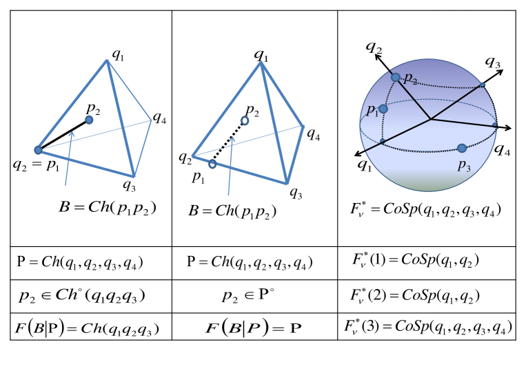
Figure 4. Essential Faces.

Lemma 4.8.

Let $\mathbb{P}$ be a polyhedron such that $\mathbb{B}\cap\mathbb{P}^{\circ}\neq\emptyset$. Then

$$F(\mathbb{B}|\mathbb{P})=\mathbb{P}.$$

Proof.

We see that $F(\mathbb{B}|\mathbb{P})\preceq\mathbb{P}$. Assume that $F(\mathbb{B}|\mathbb{P})\precneqq\mathbb{P}$. Then $\mathbb{B}\subset F(\mathbb{B}|\mathbb{P})\subset\partial\mathbb{P}$. This is a contradiction to the hypothesis $\mathbb{B}\cap\mathbb{P}^{\circ}\neq\emptyset$. ∎

Lemma 4.9.

Let $\mathbb{P}$ be a polyhedron such that $\mathbb{B}\subset\mathbb{P}$. Then

$$(F(\mathbb{B}|\mathbb{P}))^{\circ}\cap\text{Ch}(\mathbb{B})\neq\emptyset.$$

Proof.

If not, $\text{Ch}(\mathbb{B})\subset\partial F(\mathbb{B}|\mathbb{P})$. By Lemma 2.3, $\text{Ch}(\mathbb{B})\subset\mathbb{G}\precneqq F(\mathbb{B}|\mathbb{P})$, which is impossible by Definition 4.2. ∎

Lemma 4.10.

Let $\mathbb{P}$ be a polyhedron in $\mathbb{R}^{n}$ and let $\mathbb{B}\subset\mathbb{P}$ be a convex set. Then

$$\mathbb{B}^{\circ}\subset F(\mathbb{B}|\mathbb{P})^{\circ}.$$

Proof.

We need the following observation: If two affine spaces $V_{1}$ and $V_{2}$ meet at $z\in V_{1}\cap V_{2}$ with $V_{1}\nsubseteq V_{2}$ (transversally), then

(4.28) $$B_{V_{1}}(z,\epsilon)\cap(V_{2}^{+})^{\circ}\neq\emptyset B_{V_{1}}(z,\epsilon)\cap(V_{2}^{-})^{\circ}\neq\emptyset \epsilon>0$$ and for any

where $B_{V_{1}}(z,\epsilon)=\{v\in V_{1}:|v-z|<\epsilon\}$ is an $\epsilon$-neighborhood of $z$ in $V_{1}$. Let $z\in\mathbb{B}^{\circ}$. Then we show that $z\in(F(\mathbb{B}|\mathbb{P}))^{\circ}$. Since $z\in\mathbb{B}^{\circ}\subset\mathbb{B}\subset F(\mathbb{B}|\mathbb{P})$, it suffices to prove that $z\in\partial F(\mathbb{B}|\mathbb{P})$ leads to a contradiction that $z\notin\mathbb{B}^{\circ}$. If $z\in\partial F(\mathbb{B}|\mathbb{P})$, then by Definition 2.8, $z\in\mathbb{G}\precneqq F(\mathbb{B}|\mathbb{P})$ where $\mathbb{G}\subset\partial F(\mathbb{B}|\mathbb{P})$. Let $V_{am}(\mathbb{G})$ be the plane containing $\mathbb{G}$ with

(4.29) $$\text{dim}(V_{am}(\mathbb{G}))=k-1\leq k=\text{dim}(F(\mathbb{B}|\mathbb{P}))\ \text{and}\ F(\mathbb{B}|\mathbb{P})\subset V_{am}^{+}(\mathbb{G}).$$

By Definition 4.2 and Lemma 4.9, $\mathbb{B}\cap F(\mathbb{B}|\mathbb{P})^{\circ}\neq\emptyset$, that is, $V_{am}(\mathbb{B})\nsubseteq V_{am}(\mathbb{G})$. From $z\in\mathbb{B}^{\circ}$ and $z\in\mathbb{G}$, it follows that $z\in V_{am}(\mathbb{B})\cap V_{am}(\mathbb{G})$. By (4.28) and (4.29) with $V_{1}=V_{am}(\mathbb{B})$ and $V_{2}=V_{am}(\mathbb{G})$,

$$B_{V_{am}(\mathbb{B})}(z,\epsilon)\nsubseteq F(\mathbb{B}|\mathbb{P}),\ \ \text{which implies that}\ \ B_{V_{am}(\mathbb{B})}(z,\epsilon)\nsubseteq\mathbb{B}\ \ \text{for any $\epsilon>0$.}$$

This means that $z\notin\mathbb{B}^{\circ}$. ∎

5. Preliminaries Estimates

In this section, we prove Proposition 5.1, which is an elementary tool for the $L^{p}$ estimation driven by the finite type conditions in the same spirit of [6] and [21]. Proposition 5.1 and Proposition 3.1 are two basic $L^{p}$ estimation tools used for the proof of sufficiency parts of Main Theorems 1-3.

5.1. Preliminary Inequalities

Under the same setting as in the definition of multiple Hilbert transforms (1.1), we consider the multi-parameter maximal function

(5.1) $$\mathcal{M}_{\Lambda}f(x)=\sup_{r_{1},\cdots,r_{n}>0}\,\frac{1}{r_{1}\cdots r_{n}}\,\int_{-r_{1}}^{r_{1}}\cdots\int_{-r_{n}}^{r_{n}}\,\left|f\left(x-P_{\Lambda}(t)\right)\right|\,dt$$

defined for each locally integrable function $f$ on $\mathbb{R}^{d}$.

Theorem 5.1.

For $\,1<p\leq\infty\,,$ $\mathcal{M}_{\Lambda}$ is a bounded operator from $L^{p}(\mathbb{R}^{d})$ into itself and there exists a bound $C_{p}$ depending only on $\,p,n,d\,$ and the maximal degree of the polynomials $P_{\nu}$ such that

$$\left\|\,\mathcal{M}_{\Lambda}f\,\right\|_{L^{p}(\mathbb{R}^{d})}\,\leq\,C_{p}\,\|f\|_{L^{p}(\mathbb{R}^{d})}\,.$$

Remark 5.1.

This result can be proved by combining a theorem of Ricci and Stein ([17], Theorem 7.1) and the so-called lifting argument (see Chapter 11 of [18]).

Remark 5.2.

B. Street in [20] showed the $L^{p}$ boundedness for a variable coefficient version of $\mathcal{M}_{\Lambda}$ associated with analytic functions. Furthermore, A. Nagel and M. Pramanik in [11] obtain the $L^{p}$ boundedness for a different kind of multi-parameter maximal operators, that were motivated by the study of several complex variables. This maximal average is taken over family of sets (balls) that are defined by finite number of monomial inequalities. In particular, to establish the $L^{p}$ theory in [11], the geometric properties of the associated polyhedra are also systematically studied.

Take a function $\,\psi\in C^{\infty}_{c}([-2,2])\,$ such that $\,0\leq\psi\leq 1\,$ and $\,\psi(u)=1\,$ for $\,|u|\leq 1/2\,.$ Put $\,\eta(u)=\psi(u)-\psi(2u)\,.$ Given an integer $k\in\mathbb{Z}$ and $\,\alpha,\beta,\gamma\in\{1,\cdots,n\}\,,$ we consider the measures $A_{k}^{\,\alpha,\beta}$ and $P_{k}^{\gamma}$ defined in terms of Fourier transforms

(5.2) $$\left(A_{k}^{\,\alpha,\beta}\right)\widehat{}\,(\xi)=\psi\left(\frac{\xi_{\alpha}}{2^{k}\,\xi_{\beta}}\right)\,,\quad\left(P_{k}^{\gamma}\right)\widehat{}\,(\xi)=\eta\left(2^{k}\,\xi_{\gamma}\right)\,.$$

Lemma 5.1.

Suppose that $\{\mathfrak{m}_{k}\}_{k=1}^{M},\{\mathfrak{q}_{j}\}_{j=1}^{N}\subset\mathbb{Z}^{n}\,$ where $\,{\rm{rank}}\,\left[\{\mathfrak{q}_{j}\}_{j=1}^{N}\right]=n\,.$ Given $\,\alpha_{k},\beta_{k},\gamma_{j}\in\mathbb{R}\,,$ define

(5.3) $$A_{J}=A_{J\cdot\mathfrak{m}_{1}}^{\,\alpha_{1},\beta_{1}}\ast\cdots\ast A_{J\cdot\mathfrak{m}_{M}}^{\,\alpha_{M},\beta_{M}}\quad\text{and}\quad P_{J}=P_{J\cdot\mathfrak{q}_{1}}^{\gamma_{1}}\ast\cdots\ast P_{J\cdot\mathfrak{q}_{N}}^{\gamma_{N}}$$

for each $\,J\in\mathbb{Z}^{n}\,.$ Then for $1<p<\infty$,

(5.4) $$\biggl{\|}\,\left(\sum_{J\in\mathbb{Z}^{n}}\left|P_{J}\ast f\right|^{2}\right)^{1/2}\,\biggr{\|}_{L^{p}(\mathbb{R}^{d})}\,\lesssim\,\left\|f\right\|_{L^{p}(\mathbb{R}^{d})}\,,$$

and

(5.5) $$\biggl{\|}\,\left(\sum_{J\in\mathbb{Z}^{n}}\left|A_{J}\ast P_{J}\ast f\right|^{2}\right)^{1/2}\,\biggr{\|}_{L^{p}(\mathbb{R}^{d})}\,\lesssim\,\left\|f\right\|_{L^{p}(\mathbb{R}^{d})}\,.$$

Proof.

It suffices to deal with the sum over $\mathbb{Z}^{n}_{+}$. We show (5.5). With $\left(r_{J}(t)\right)$ denoting the Rademacher functions of product form,

$$\biggl{\|}\left(\sum_{J\in\mathbb{Z}^{n}_{+}}\left|A_{J}\ast P_{J}\ast f\right|^{2}\right)^{1/2}\biggr{\|}_{L^{p}(\mathbb{R}^{d})}^{p}\,\approx\,\int_{U}\bigl{\|}\sum_{J\in\mathbb{Z}^{n}_{+}}\,r_{J}(t)\,A_{J}\ast P_{J}\ast f\bigr{\|}_{L^{p}(\mathbb{R}^{d})}^{p}dt$$

where $\,U=[0,1]^{n}\,.$ Consider the symbol

$$m(\xi)=\biggl{(}\sum_{J\in\mathbb{Z}^{n}_{+}}\,r_{J}(t)\,A_{J}\ast P_{J}\biggr{)}\,\,\,\widehat{}\,(\xi)\,.$$

Using the full rank condition for the $\mathfrak{q}_{j}$ and the support conditions, it can be shown that $m$ satisfies

$$\left|\frac{\partial^{\ell}}{\partial_{\nu_{1}}\cdots\partial_{\nu_{\ell}}}\,m(\xi_{1},\cdots,\xi_{d})\,\right|\,\leq\,\frac{C_{\ell}}{\left|\xi_{\nu_{1}}\right|\cdots\left|\xi_{\nu_{\ell}}\right|}$$

for every $\,\ell=1,\cdots,d\,,$ where $\,1\leq\nu_{1}<\cdots<\nu_{\ell}\leq d\,.$ Thus the desired conclusion follows from the multi-parameter Marcinkiewicz multiplier theorem. (5.4) follows similarly. ∎

Lemma 5.2.

Let $\,(\sigma_{J})_{J\in\mathbb{Z}^{n}}\,$ be a sequence of positive measures on $\mathbb{R}^{d}$ with the following properties :

$${\rm(i)}\quad\bigl{\|}\,\sigma_{J}\ast f\,\bigr{\|}_{L^{1}(\mathbb{R}^{d})}\,\lesssim\,\|f\|_{L^{1}(\mathbb{R}^{d})}\quad(J\in\mathbb{Z}^{n})$$

$${\rm(ii)}\quad\left\|\,\sup_{J\in\mathbb{Z}^{n}}\,\left|\sigma_{J}\ast f\right|\,\right\|_{L^{p_{0}}(\mathbb{R}^{d})}\,\lesssim\,\|f\|_{L^{p_{0}}(\mathbb{R}^{d})}$$

for some $\,1<p_{0}\leq 2\,$. Then

$$\biggl{\|}\left(\sum_{J\in\mathbb{Z}^{n}}\left|\sigma_{J}\ast f_{J}\right|^{2}\right)^{1/2}\biggr{\|}_{L^{p_{1}}(\mathbb{R}^{d})}\,\lesssim\,\biggl{\|}\left(\sum_{J\in\mathbb{Z}^{n}}\left|f_{J}\right|^{2}\right)^{1/2}\biggr{\|}_{L^{p_{1}}(\mathbb{R}^{d})}$$

for $p_{1}$ determined by $\,1/p_{1}\leq 1/2\,(1+1/p_{0})\,.$

Proof.

For $\,1\leq p,\,q\leq\infty\,,$ consider the operator $T$ defined by $\,T[(f_{J})]=(\sigma_{J}\ast f_{J})\,$ on the mixed-norm spaces $L^{p}(\ell^{q})$. The condition (i) implies that $T$ maps $L^{1}(\ell^{1})$ boundedly into itself. The condition (ii) and the positivity of each $\sigma_{J}$ imply that $T$ maps $L^{p_{0}}(\ell^{\infty})$ boundedly into itself. It follows from the vector-valued Riesz-Thorin interpolation theorem that $T$ maps $L^{p_{1}}(\ell^{2})$ boundedly into itself. ∎

5.2. Basic $L^{p}$ estimates

Proposition 5.1.

Let $\{H_{J}\}_{J\in\mathbb{Z}^{d}}$ be a class of measures such that $\widehat{H}_{J}$ be the Fourier multiplier of $H_{J}$. Suppose that

(5.6) $$\left|\widehat{H}_{J}(\xi)\right| \leq C\min\left\{\left|2^{-J\cdot\mathfrak{q}_{i}}\xi_{\nu_{i}}\right|^{-\delta_{1}},\left|2^{-J\cdot\mathfrak{q}_{i}}\xi_{\nu_{i}}\right|^{\delta_{2}}:i=1,\cdots,N\right\}$$

where

(5.7) $$\text{rank}\{\mathfrak{q}_{i}:i=1,\cdots,r\}=n.$$

Then for $C_{2}=C/(1-2^{-\min\{\delta_{1},\delta_{2}\}/N})^{N}$ with $C,\delta_{1},\delta_{2},N$ in (5.6),

(5.8) $$\sum_{J\in Z}\left|\widehat{H}_{J}(\xi)\right|\leq C_{2}\ \ \text{where}\ Z\subset\mathbb{Z}^{n}$$

which implies that for $A_{J}$ of the form defined as in (5.3) and for any $Z\subset\mathbb{Z}^{n}$,

$$\left\|\sum_{J\in Z}H_{J}*A_{J}*f\right\|_{L^{2}(\mathbb{R}^{d})}\leq C_{2}\left\|f\right\|_{L^{2}(\mathbb{R}^{d})}.$$

Moreover, suppose that $1<p\leq\infty$

(5.9) $$\left\|\sup_{J\in Z}|H_{J}|*f\right\|_{L^{p}(\mathbb{R}^{d})}\leq C\left\|f\right\|_{L^{p}(\mathbb{R}^{d})}.$$

Then, for $1<p\leq\infty$

(5.10) $$\left\|\sum_{J\in Z}H_{J}*A_{J}*f\right\|_{L^{p}(\mathbb{R}^{d})}\leq C_{p}\left\|f\right\|_{L^{p}(\mathbb{R}^{d})}.$$

Proof of (5.8).

Let

$$\big{(}P_{-J\cdot\mathfrak{q}_{i}-\ell_{i}}\big{)}^{\wedge}(\xi) = \eta\left(2^{-J\cdot\mathfrak{q}_{i}-\ell_{i}}\,\xi_{\nu_{i}}\right)\quad\text{for}\quad i=1,\cdots,N\,$$

with a view to restricting frequency variables as

(5.11) $$2^{-J\cdot\mathfrak{q}_{i}}\,\left|\xi_{\nu_{i}}\right|\, \approx \,2^{\ell_{i}}\quad\text{for}\quad i=1,\cdots,N\,.$$

We use for (5.6) and (5.11) to obtain that

(5.12) $$\qquad\prod_{i=1}^{N}\eta\left(2^{-J\cdot\mathfrak{q}_{i}-\ell_{i}}\,\xi_{\nu_{i}}\right)\left|\widehat{H}_{J}(\xi)\right|\,\leq\,C2^{-b\,|L|}\ \text{for }\ b=\frac{\min\{\delta_{1},\delta_{2}\}}{N}\,\ \text{and}\ C\ \text{ in (\ref{jr1v})}.$$

where $|L|=\sum_{i=1}^{N}|\ell_{i}|$. Then by using positivity of $\eta$ and $\sum_{\ell_{i}\in\mathbb{Z}}\eta\left(2^{-J\cdot\mathfrak{q}_{i}-\ell_{i}}\,\xi_{\nu_{i}}\right)=1$,

$$\sum_{|J|\leq R}\left|\widehat{H}_{J}(\xi)\right| = \sum_{L\in\mathbb{Z}^{N}}\prod_{i=1}^{N}\eta\left(2^{-J\cdot\mathfrak{q}_{i}-\ell_{i}}\,\xi_{\nu_{i}}\right)\sum_{|J|\leq R}\left|\widehat{H}_{J}(\xi)\right|$$

$$= \sum_{L\in\mathbb{Z}^{N}}\sum_{|J|\leq R}\prod_{i=1}^{N}\eta\left(2^{-J\cdot\mathfrak{q}_{i}-\ell_{i}}\,\xi_{\nu_{i}}\right)\left|\widehat{H}_{J}(\xi)\right|$$

$$\leq \sum_{L\in\mathbb{Z}^{N}}C2^{-b\,|L|}\leq C/(1-2^{-\min\{\delta_{1},\delta_{2}\}/N})^{N}$$

where the first inequality follows from (5.12) and the observation that for each fixed $\xi$, there exists finitely many $J$ such that $\prod_{i=1}^{N}\eta\left(2^{-J\cdot\mathfrak{q}_{i}-\ell_{i}}\,\xi_{\nu_{i}}\right)\neq 0$. We proved (5.8). ∎

Proof of (5.10).

Define

$$\mathcal{P}_{J,L}^{\mathfrak{q}}=P_{-J\cdot\mathfrak{q}_{1}-\ell_{1}}*\cdots*P_{-J\cdot\mathfrak{q}_{N}-\ell_{N}}\,,\ \text{where}\ \ L=(\ell_{i})_{i=1}^{N}\in\mathbb{Z}^{N}.$$

We use the Littlewood-Paley decomposition for each $J\in\mathbb{Z}$:

$$\sum_{L\in\mathbb{Z}^{N}}\mathcal{P}_{J,L}^{\mathfrak{q}}\ast f=f.$$

Define $\tilde{\mathcal{P}}_{J,L}^{\mathfrak{q}}$ by replacing $\eta(\cdot)$ with $\eta(\cdot/2)$ in (5.2). Then $\tilde{\mathcal{P}}_{J,L}^{\mathfrak{q}}*\mathcal{P}_{J,L}^{\mathfrak{q}}=\mathcal{P}_{J,L}^{\mathfrak{q}}$. Thus

$$\sum_{J\in Z}H_{J}*A_{J}*\mathcal{P}_{J,L}^{\mathfrak{q}}*f=\sum_{J\in Z}\tilde{\mathcal{P}}_{J,L}^{\mathfrak{q}}*H_{J}*A_{J}*\mathcal{P}_{J,L}^{\mathfrak{q}}*f.$$

By Applying the dual inequality of (5.4) in Lemma 5.1,

$$\left\|\sum_{J\in Z}\tilde{\mathcal{P}}_{J,L}^{\mathfrak{q}}*H_{J}*A_{J}*\mathcal{P}_{J,L}^{\mathfrak{q}}*f\right\|_{L^{p}(\mathbb{R}^{d})}\leq\biggl{\|}\biggl{(}\sum_{J\in Z}\left|H_{J}*A_{J}*\mathcal{P}_{J,L}^{\mathfrak{q}}*f\right|^{2}\biggr{)}^{1/2}\biggl{\|}_{L^{p}(\mathbb{R}^{d})}.$$

Thus, it is sufficient to find a constant $\,b>0\,$ independent of $L\in\mathbb{Z}^{N}\,$ such that

(5.13) $$\biggl{\|}\biggl{(}\sum_{J\in Z}\left|H_{J}*A_{J}*\mathcal{P}_{J,L}^{\mathfrak{q}}*f\right|^{2}\biggr{)}^{1/2}\biggl{\|}_{L^{p}(\mathbb{R}^{d})}\,\leq\,\tilde{C}2^{-b\,|L|}\|f\|_{L^{p}(\mathbb{R}^{d})}\,,$$

where $\tilde{C}$ is a multiple of $C$ in (5.6). By the rank condition (5.7) and (5.5) in Lemma 5.1,

(5.14) $$\biggl{\|}\Bigl{(}\sum_{J\in Z}|A^{\sigma}_{J}*\mathcal{P}_{J,L}^{\mathfrak{q}}*f|^{2}\Bigl{)}^{\frac{1}{2}}\biggl{\|}_{L^{p}(\mathbb{R}^{d})} \lesssim \parallel f\parallel_{L^{p}(\mathbb{R}^{d})}.$$

For $p=2$, we use (5.8),(5.12) and (5.14) to obtain (5.13). Applying a standard bootstrap argument combined with (5.9), Lemmas 5.1 and 5.2, we obtain (5.13) for the other values of $p\neq 2$. The proof of (5.10) is now complete. ∎

Remark 5.3.

The decay condition in (5.6) always holds for the case that $\Lambda_{\nu}$’s are mutually disjoint. Given $\mathbb{G}=(\mathbb{G}_{\nu})\in\mathcal{F}({\bf N}(\Lambda,S))$, we have from the multi-dimensional Van der Corput Lemma,

(5.15) $$|\mathcal{I}_{J}(P_{\mathbb{G}},\xi)|\leq C\min\left\{|2^{-J\cdot\mathfrak{m}_{\nu}}\xi_{\nu}|^{-\delta},1:\mathfrak{m}_{\nu}\in\mathbb{G}_{\nu}\cap\Lambda_{\nu}\ \text{for}\ \nu=1,\cdots,d\right\}.$$

6. Cone Type Decompositions

6.1. Cone Decompositions

Recall that $Z(S)=\prod Z_{i}$ with $Z_{i}=\mathbb{R}_{+}$ for $i\in S$ and $Z_{i}=\mathbb{R}$ for $i\in N_{n}\setminus S$ as in Definition 2.14. We decompose $Z(S)$ into finite number of different cones that appears in (2.12) and (2.15) as follows:

Proposition 6.1.

Let $\Lambda=(\Lambda_{\nu})$ with $\Lambda_{\nu}\subset\mathbb{Z}_{+}^{n}$ and $S\subset\{1,\cdots,n\}$. Then,

$$\bigcup_{\mathbb{F}\in\mathcal{F}\left(\vec{{\bf N}}(\Lambda,S)\right)}{\rm Cap}(\mathbb{F}^{*})=Z(S)\ \text{where}\ \rm{Cap}(\mathbb{F}^{*})=\bigcap_{\nu=1}^{d}\mathbb{F}_{\nu}^{*}\ \text{for}\ \mathbb{F}=(\mathbb{F}_{\nu})\in\mathcal{F}({\bf N}(\Lambda,S)).$$

Moreover,

$$\bigcup_{\mathbb{F}\in\mathcal{F}\left(\vec{{\bf N}}(\Lambda,S)\right)}{\rm Cap}((\mathbb{F}^{*})^{\circ})=Z(S)\setminus\{0\}\ \text{where}\ \rm{Cap}((\mathbb{F}^{*})^{\circ})=\bigcap_{\nu=1}^{d}(\mathbb{F}_{\nu}^{*})^{\circ}.$$

Lemma 6.1.

Let $\mathbb{P}=\mathbb{P}(\Pi)$ with $\Pi=\{\pi_{\mathfrak{q}_{j},r_{j}}:j=1,\cdots,N\}$ be a polyhedron. Then

$$\inf\{\langle{\bf x},{\bf e}\rangle:{\bf x}\in\mathbb{P}\}>-\infty\ \ \text{if and only if}\ \ {\bf e}\in\rm{CoSp}(\{\mathfrak{q}_{j}:j=1,\cdots,N\}).$$

Proof.

Let $\rho=\inf\{\langle{\bf x},{\bf e}\rangle:{\bf x}\in\mathbb{P}\}>-\infty$ and set the plane $\pi_{{\bf e},\rho}=\{{\bf x}\in V:\langle{\bf x},{\bf e}\rangle=\rho\}$. Since $\mathbb{P}$ is a closed set, $\mathbb{F}$ defined by $\pi_{{\bf e},\rho}\cap\mathbb{P}$ is a non-empty closed set. From $\rho\leq{\bf x}\cdot{\bf e}$ for all ${\bf x}\in\mathbb{P}$ and $\mathbb{F}=\pi_{{\bf e},\rho}\cap\mathbb{P}$,

(6.1) $$\mathbb{P}\setminus\mathbb{F}\subset\left(\pi_{{\bf e},\rho}^{+}\right)^{\circ}.$$

Thus $\mathbb{F}\preceq\mathbb{P}$ and ${\bf e}\in\mathbb{F}^{*}\subset\rm{CoSp}(\{\mathfrak{q}_{j}:j=1,\cdots,N\})$ by using Propositions 4.1 and 4.2. To show the other direction, let ${\bf e}=\sum_{j=1}^{N}c_{j}\mathfrak{q}_{j}\in\rm{CoSp}(\{\mathfrak{q}_{j}:j=1,\cdots,N\})$. Then

$$\langle{\bf e},{\bf x}\rangle=\sum_{j=1}^{N}c_{j}\langle\mathfrak{q}_{j},{\bf x}\rangle\geq\sum_{j=1}^{N}c_{j}r_{j}>-\infty$$

for all ${\bf x}\in\mathbb{P}=\bigcap_{j=1}^{N}\{\langle\mathfrak{q}_{j},{\bf x}\rangle\geq r_{j}:j=1,\cdots,N\}$. ∎

Lemma 6.2.

Let $\mathbb{P}=\mathbb{P}(\Pi)$ with $\Pi=\{\pi_{\mathfrak{q}_{j},r_{j}}:j=1,\cdots,N\}$ be a polyhedron. Then

$$\rm{CoSp}(\{\mathfrak{q}_{j}:j=1,\cdots,N\})=\bigcup_{\mathbb{F}\preceq\mathbb{P}}\mathbb{F}^{*}.$$

Proof.

We first show $\subset$. Let ${\bf e}=\sum_{j=1}^{N}c_{j}\mathfrak{q}_{j}\in\rm{CoSp}(\{\mathfrak{q}_{j}:j=1,\cdots,N\})$ and let

$$\rho=\inf\left\{\langle{\bf e},{\bf x}\rangle=\sum_{j=1}^{N}c_{j}\langle\mathfrak{q}_{j},{\bf x}\rangle:{\bf x}\in\mathbb{P}\right\}$$

that exits from Lemma 6.1. Set $\mathbb{F}=\pi_{{\bf e},\rho}\cap\mathbb{P}$. By (6.1), $\mathbb{F}$ is a face of $\mathbb{P}$ with a supporting plane $\pi_{{\bf e},\rho}$. Thus ${\bf e}\in\mathbb{F}^{*}$. The other direction $\supset$ follows from Propositions 4.1 and 4.2. ∎

Lemma 6.3.

Let ${\bf u}=(u_{1},\cdots,u_{n})\in\mathbb{F}^{*}$ and $\mathbb{F}\in\mathcal{F}({\bf N}(\Lambda,S))$. Then $u_{j}\geq 0$ for all $j\in S$.

Proof.

Let $\mathfrak{m}\in\mathbb{F}$ and $j\in S$. Then $\mathfrak{m}+r{\bf e}_{j}\in{\bf N}(\Lambda,S)$ for all $r\geq 0$. By Definition 2.8 and ${\bf u}\in\mathbb{F}^{*}$, $u_{j}r=\langle{\bf u},\mathfrak{m}+r{\bf e}_{j}-\mathfrak{m}\rangle\geq 0$. Thus $u_{j}\geq 0$. See Figure 1. ∎

Lemma 6.4.

Let $S\subset N_{n}$ and $\Omega\subset\mathbb{Z}_{+}^{n}$ be a finite set. Suppose that $\mathbb{P}=\mathbb{P}(\Pi)$ with $\Pi=\{\pi_{\mathfrak{q}_{j},r_{j}}:j=1,\cdots,N\}$ is a polyhedron given by ${\bf N}(\Omega,S)$. Then

$$\bigcup_{\mathbb{F}\in\mathcal{F}\left({\bf N}(\Omega,S)\right)}\mathbb{F}^{*}=Z(S).$$

Moreover, $\bigcup_{\mathbb{F}\in\mathcal{F}\left({\bf N}(\Omega,S)\right)}(\mathbb{F}^{*})^{\circ}=Z(S)\setminus\{0\}$.

Proof.

It follows $\subset$ from Lemma 6.3. We next show $\supset$. Put

$$m_{k} = \min\{u_{k}:{\bf u}=(u_{1},\cdots,u_{n})\in\Omega\},$$

$$M_{k} = \max\{u_{k}:{\bf u}=(u_{1},\cdots,u_{n})\in\Omega\}$$

By ${\bf N}(\Omega,S)=\rm{Ch}\{{\bf u}+\mathbb{R}_{+}^{S}:{\bf u}\in\Omega\}$,

• if $k\in N_{n}\setminus S$, then $m_{k}\leq x_{k}\leq M_{k}$ for all ${\bf x}=(x_{1},\cdots,x_{n})\in{\bf N}(\Omega,S)$,

• if $k\in S$, then $m_{k}\leq x_{k}$ for all ${\bf x}=(x_{1},\cdots,x_{n})\in{\bf N}(\Omega,S)$.

Thus, if $k\in N_{n}\setminus S$, then ${\bf e}_{k},-{\bf e}_{k}\in\rm{CoSp}(\{\mathfrak{q}_{j}:j=1,\cdots,N\})$ by Lemma 6.1 and (1) above. If $k\in S$, then ${\bf e}_{k}\in\rm{CoSp}(\{\mathfrak{q}_{j}:j=1,\cdots,N\})$ by Lemma 6.1 and (2) above. Hence

$$Z(S)=\rm{CoSp}(\{\pm{\bf e}_{k}:k\in N_{n}\setminus S\}\cup\{{\bf e}_{k}:k\in S\})\subset\rm{CoSp}(\{\mathfrak{q}_{j}:j=1,\cdots,N\}).$$

By Lemma 6.2, $Z(S)\subset\bigcup_{\mathbb{F}\in\mathcal{F}\left({\bf N}(\Omega,S)\right)}\mathbb{F}^{*}$. By Definitions 2.8-2.10 together with (4.22),

(6.2) $$\bigcup_{\mathbb{F}\in\mathcal{F}\left({\bf N}(\Omega,S)\right)}(\mathbb{F}^{*})^{\circ}=\bigcup_{\mathbb{F}\in\mathcal{F}\left({\bf N}(\Omega,S)\right)}\mathbb{F}^{*}\setminus\{0\}.$$

This implies the last statement. ∎

Proof of Proposition 6.1.

By Lemma 6.4,

$$\bigcup_{\mathbb{F}_{\nu}\in\mathcal{F}({\bf N}(\Lambda_{\nu},S))}\mathbb{F}_{\nu}^{*}=Z(S)\ \ \text{for every $\nu=1,\cdots,d$}.$$

Hence, by taking an intersection for $\nu=1,\cdots,d$,

$$\bigcup_{\mathbb{F}\in\mathcal{F}\left(\vec{{\bf N}}(\Lambda,S)\right)}{\rm Cap}(\mathbb{F}^{*})=\bigcap_{\nu=1}^{d}\bigcup_{\mathbb{F}_{\nu}\in\mathcal{F}({\bf N}(\Lambda_{\nu},S))}\mathbb{F}_{\nu}^{*}=Z(S).$$

The last statement follows from (6.2). ∎

6.2. Projection to Sphere; Boundary Deleted Neighborhood

We show that

Proposition 6.2.

Suppose that $\text{rank}\left(\bigcup_{\nu=1}^{d}{\bf N}(\Lambda_{\nu},S)\right)\leq n-1$ and the hypothesis of Main Theorems 2 holds. Then for $1<p<\infty$,

$$\left\|\sum_{J\in Z(S)}H^{P_{\Lambda}}_{J}*f\right\|_{L^{p}(\mathbb{R}^{d})}\,\lesssim\,\left\|f\right\|_{L^{p}(\mathbb{R}^{d})}$$

where $\mathcal{I}_{J}(P_{\Lambda},\xi)=\left(H^{P_{\Lambda}}_{J}\right)^{\wedge}(\xi)$.

To show Proposition 6.2, we consider the projective cone of $\mathbb{F}^{*}$ to the sphere $\mathbb{S}^{n-1}$.

Definition 6.1.

In stead of working with the cone $\mathbb{F}^{*}$ of a face $\mathbb{F}$, it is sometimes convenient to work with its intersection $\mathbb{F}^{*}\cap\mathbb{S}^{n-1}$ with the sphere. We denote it and its boundary by

$$\mathbb{S}[\mathbb{F}^{*}]=\mathbb{F}^{*}\cap\mathbb{S}^{n-1}\ \ \text{and}\ \ \partial\mathbb{S}[\mathbb{F}^{*}]=(\partial\mathbb{F}^{*})\cap\mathbb{S}^{n-1}.$$

Let $K\in\mathbb{S}^{n-1}$, then we define the $\epsilon$-neighborhood of $K$ by

$$N_{\epsilon}(K)=\{x\in\mathbb{S}^{n-1}:|x-y|<\epsilon\ \text{for some $y\in K$}\}.$$

Definition 6.2.

[Boundary Deleted $\epsilon$-neighborhood of $\mathbb{S}[\mathbb{F}^{*}]$ Let $\mathbb{P}$ be a polyhedron in $\mathbb{R}^{n}$ of $\text{dim}(\mathbb{P})=m<n$ and let $\mathbb{S}[\mathbb{F}^{*}]\in\mathbb{S}^{n-1}$ with $\mathbb{F}\in\mathcal{F}^{m-k}(\mathbb{P})$ where $k=0,\cdots,m$. To give some width to $\mathbb{S}[\mathbb{F}^{*}]\setminus N_{\epsilon}(\partial\mathbb{S}[\mathbb{F}^{*}]))$, we define a boundary deleted $\epsilon$-neighborhood $\mathbb{S}_{\epsilon}[\mathbb{F}^{*}]$ by

$$\mathbb{S}_{\epsilon}[\mathbb{F}^{*}] = N_{\epsilon/M^{k}}\left(\mathbb{S}[\mathbb{F}^{*}])\right)\ \ \text{for $k=0$ where $\mathbb{F}^{*}=\text{CoSp}(\Pi_{b})=V^{\perp}(\mathbb{P})$}\,,$$

$$\mathbb{S}_{\epsilon}[\mathbb{F}^{*}] = N_{\epsilon/M^{k+1/3}}\left(\mathbb{S}[\mathbb{F}^{*}]\setminus N_{\epsilon/M^{k-1/3}}(\partial\mathbb{S}[\mathbb{F}^{*}])\right)\ \ \text{for $1\leq k\leq m$ }$$

where $\mathbb{F}^{*}=\text{CoSp}(\Pi_{a}(\mathbb{F}))\oplus V^{\perp}(\mathbb{P})=\text{CoSp}(\{\mathfrak{q}_{j}\}_{j=1}^{\ell})\oplus V^{\perp}(\mathbb{P})$ as in (4.21). Here $M$ will be chosen to be a large positive number. For the case that $\text{dim}(\mathbb{P})=n$ with $\mathbb{F}\in\mathcal{F}^{m-k}(\mathbb{P})$ where $k=1,\cdots,n$, we define a boundary deleted $\epsilon$-neighborhood $\mathbb{S}_{\epsilon}[\mathbb{F}^{*}]$ by

$$\mathbb{S}_{\epsilon}[\mathbb{F}^{*}] = N_{\epsilon/M^{k}}\left(\mathbb{S}[\mathbb{F}^{*}])\right)\ \ \text{for $k=1$ where $\mathbb{F}^{*}=\text{CoSp}(\mathfrak{q}_{j})$}\,,$$

$$\mathbb{S}_{\epsilon}[\mathbb{F}^{*}] = N_{\epsilon/M^{k+1/3}}\left(\mathbb{S}[\mathbb{F}^{*}]\setminus N_{\epsilon/M^{k-1/3}}(\partial\mathbb{S}[\mathbb{F}^{*}])\right)\ \ \text{for $2\leq k\leq n$ }$$

where $\mathbb{F}^{*}=\text{CoSp}(\{\mathfrak{q}_{j}\}_{j=1}^{\ell})$. See $\mathbb{S}_{\epsilon}[\mathbb{F}^{*}(\mathfrak{q}_{1})]$ and $\mathbb{S}_{\epsilon}[\mathbb{F}^{*}(\mathfrak{q}_{1},\mathfrak{q}_{4})]$ in the right side of Figure 3.

Lemma 6.5.

Let $\Omega\subset\mathbb{Z}_{+}^{n}$ and $\mathbb{P}={\bf N}(\Omega,S)\subset\mathbb{R}^{n}$ be a polyhedron. Then

$$\bigcup_{\mathbb{F}\in\mathcal{F}({\bf N}(\Omega,S))}\mathbb{S}[\mathbb{F}^{*}]\subset\bigcup_{\mathbb{F}\in\mathcal{F}({\bf N}(\Omega,S))}\mathbb{S}_{\epsilon}[\mathbb{F}^{*}].$$

Proof.

We prove the case $\text{dim}(\mathbb{P})=m<n$. By Definition 6.2,

$$\bigcup_{\mathbb{F}\in\mathcal{F}^{m}({\bf N}(\Omega,S))}\mathbb{S}[\mathbb{F}^{*}]\subset\bigcup_{\mathbb{F}\in\mathcal{F}^{m}({\bf N}(\Omega,S))}\mathbb{S}_{\epsilon}[\mathbb{F}^{*}]=\bigcup_{\mathbb{F}\in\mathcal{F}^{m}({\bf N}(\Omega,S))}N_{\epsilon/M}\left(\mathbb{S}[\mathbb{F}^{*}]\right).$$

Using this and Definition 6.2,

$$\bigcup_{\mathbb{F}\in\mathcal{F}^{m-1}({\bf N}(\Omega,S))}\mathbb{S}[\mathbb{F}^{*}]\subset\left(\bigcup_{\mathbb{F}\in\mathcal{F}^{m-1}({\bf N}(\Omega,S))}\mathbb{S}_{\epsilon}[\mathbb{F}^{*}]\right)\cup\left(\bigcup_{\mathbb{F}\in\mathcal{F}^{m}({\bf N}(\Omega,S))}\mathbb{S}_{\epsilon}[\mathbb{F}^{*}]\right).$$

Inductive application of this inclusion completes the proof. ∎

Note that by Proposition 6.1,

(6.3) $$\bigcup_{\mathbb{F}=(\mathbb{F}_{\nu})\in\mathcal{F}\left(\vec{{\bf N}}(P,S)\right)}\bigcap_{\nu=1}^{d}\mathbb{S}[\mathbb{F}^{*}_{\nu}]=Z(S)\cap\mathbb{S}^{n-1}.$$

By Lemma 6.5 together with (6.3), we have

Lemma 6.6.

Let $\Lambda=(\Lambda_{\nu})$ with $\Lambda_{\nu}\subset\mathbb{Z}_{+}^{n}$ and $\vec{{\bf N}}(\Lambda,S)=\left({\bf N}(\Lambda_{\nu},S)\right)$. Then

$$Z(S)\cap\mathbb{S}^{n-1}\subset\bigcup_{\mathbb{F}=(\mathbb{F}_{\nu})\in\mathcal{F}(\vec{{\bf N}}(\Lambda,S))}\bigcap_{\nu=1}^{d}\mathbb{S}_{\epsilon}[\mathbb{F}^{*}_{\nu}].$$

Using this we can decompose for sufficiently small $\epsilon>0$,

(6.4) $$\sum_{J\in Z(S)}H^{P_{\Lambda}}_{J}=\sum_{\mathbb{F}\in\mathcal{F}(\vec{{\bf N}}(\Lambda,S))}\sum_{J/|J|\in Z\subset\bigcap_{\nu=1}^{d}\mathbb{S}_{\epsilon}[\mathbb{F}^{*}_{\nu}]}H^{P_{\Lambda}}_{J}.$$

In order to check the overlapping condition (3.3), we need the following lemma.

Lemma 6.7.

Let $\mathbb{F}_{\nu}\in\mathcal{F}({\bf N}(\Lambda_{\nu},S))$ for $\nu=1,\cdots,d$. Then for some sufficiently small $\epsilon>0$, we have the property that $\bigcap_{\nu=1}^{d}\mathbb{S}_{\epsilon}[\mathbb{F}^{*}_{\nu}]\neq\emptyset$ implies that $\bigcap_{\nu=1}^{d}\mathbb{S}[(\mathbb{F}^{*}_{\nu})^{\circ}]\neq\emptyset$.

Proof of lemma 6.7.

We prove the case $\text{dim}(\mathbb{P})=m<n$. It suffices to find an $\epsilon>0$ such that

$$\bigcap_{\nu=1}^{d}\mathbb{S}[(\mathbb{F}^{*}_{\nu})^{\circ}]=\emptyset\ \ \text{implies that}\ \ \bigcap_{\nu=1}^{d}\mathbb{S}_{\epsilon}[\mathbb{F}^{*}_{\nu}]=\emptyset.$$

Suppose that $d$-tuple $(\mathbb{F}_{\nu})$ of faces are given so that

(6.5) $$\bigcap_{\nu=1}^{d}\mathbb{S}[(\mathbb{F}^{*}_{\nu})^{\circ}]=\emptyset.$$

Note that $\mathbb{S}[\mathbb{F}^{*}_{\nu}]\setminus N_{\epsilon}(\partial\mathbb{S}[\mathbb{F}^{*}_{\nu}])\subset\mathbb{S}[(\mathbb{F}^{*}_{\nu})^{\circ}]$ for any positive number $\epsilon>0$ and $\mathbb{S}[\mathbb{F}^{*}_{\nu}]=\mathbb{S}[(\mathbb{F}^{*}_{\nu})^{\circ}]$ for $\text{dim}(\mathbb{F}_{\nu})=m$. From this, we splits (6.5) into two smaller parts:

(6.6) $$\bigcap_{\nu;\,\text{dim}(\mathbb{F}_{\nu})\leq m-1}\left(\mathbb{S}[\mathbb{F}^{*}_{\nu}]\setminus N_{\epsilon/M^{k(\nu)-1/3}}(\partial\mathbb{S}[\mathbb{F}^{*}_{\nu}])\right)\bigcap\bigcap_{\nu;\,\text{dim}(\mathbb{F}_{\nu})=m}\mathbb{S}[\mathbb{F}^{*}_{\nu}]\subset\bigcap_{\nu=1}^{d}\mathbb{S}[(\mathbb{F}^{*}_{\nu})^{\circ}]=\emptyset.$$

Since $\mathbb{S}[\mathbb{F}^{*}_{\nu}]$ and $\mathbb{S}[\mathbb{F}^{*}_{\nu}]\setminus N_{\epsilon/M^{k(\nu)-1/3}}(\partial\mathbb{S}[\mathbb{F}^{*}_{\nu}])$ are closed sets in $\mathbb{S}^{n-1}$ in (6.6), we take a little bit thicker intersection in $\nu=1,\cdots,d$ with some large $M$ and small $\epsilon$ to obtain that

$$\bigcap_{\nu;\,\text{dim}(\mathbb{F}_{\nu})\leq m-1}N_{\epsilon/M^{k(\nu)+1/3}}\left(\mathbb{S}[\mathbb{F}^{*}_{\nu}]\setminus N_{\epsilon/M^{k(\nu)-1/3}}(\partial\mathbb{S}[\mathbb{F}^{*}_{\nu}])\right)\bigcap\bigcap_{\nu;\,\text{dim}(\mathbb{F}_{\nu})=m}\mathbb{S}_{\epsilon/M}[\mathbb{F}^{*}_{\nu}]=\emptyset.$$

By Definition 6.2, we have

$$\bigcap_{\nu}\mathbb{S}_{\epsilon}[\mathbb{F}^{*}_{\nu}]=\emptyset.$$

This proves Lemma 6.7. The case $\text{dim}(\mathbb{P})=n$ follows similarly. ∎

Lemma 6.8.

Let $\mathbb{F}$ be a face of $\mathbb{P}={\bf N}(\Omega,S)$ with $\text{dim}(\mathbb{P})=m<n$. Suppose that $\tilde{\mathfrak{m}}\in\mathbb{F}\cap\Omega$ and $\mathfrak{m}\in\Omega\setminus\mathbb{F}$. Then for all $\mathfrak{p}\in\mathbb{S}_{\epsilon}[\mathbb{F}^{*}]$ with $\text{dim}(\mathbb{F})=m-k$ where $k=1,\cdots,m$,

(6.7) $$\mathfrak{p}\cdot(\mathfrak{m}-\tilde{\mathfrak{m}})\geq c>0\ \ \text{where}\ \ c\ \text{is independent of $\mathfrak{p}$}.$$

Remark 6.1.

We shall use Lemma 6.8 for the estimate of the difference $\mathcal{I}_{J}(P_{\Omega},\xi)-\mathcal{I}_{J}(P_{\mathbb{F}},\xi)$ where $J/|J|=\mathfrak{p}$. We do not need Lemma 6.8 if $\text{dim}(\mathbb{F})=m-k$ with $k=0$, since $\mathbb{F}={\bf N}(\Omega,S)$ for the case $\text{dim}(\mathbb{F})=m$ so that $\mathcal{I}_{J}(P_{\Omega},\xi)-\mathcal{I}_{J}(P_{\mathbb{F}},\xi)\equiv 0$. For the case $\text{dim}(\mathbb{P})=n$, (6.7) also holds for all $\mathbb{S}_{\epsilon}[\mathbb{F}^{*}]$ with $\text{dim}(\mathbb{F})=n-k$ where $k=1,\cdots,n$.

Proof of Lemma 6.1.

By Proposition 4.2,

$$\mathbb{F}^{*}=\mathbb{F}^{*}|\mathbb{P}=\text{CoSp}(\{\mathfrak{q}_{j}\}_{j=1}^{\ell}\}\cup\{\pm\mathfrak{n}_{i}\}_{i=1}^{n-m})$$

where $\{\mathfrak{q}_{j}\}_{j=1}^{\ell}$ and $\{\pm\mathfrak{n}_{i}\}_{i=1}^{n-m}$ is defined as in (4.8). Here we can take $\mathfrak{q}_{j}\in\mathbb{S}^{n-1}$. Then

$$\mathbb{S}[\mathbb{F}^{*}]=\text{CoSp}(\{\mathfrak{q}_{j}\}_{j=1}^{\ell}\}\cup\{\pm\mathfrak{n}_{i}\}_{i=1}^{n-m})\cap\mathbb{S}^{n-1}=\left\{\mathfrak{q}\in\mathbb{S}^{n-1}:\mathfrak{q}=\sum_{j}c_{j}\mathfrak{q}_{j}+\mathfrak{r}\ \text{with}\ c_{j}>0\right\}$$

where $\mathfrak{r}=\sum_{i=1}^{n-m}c_{i,\pm}\,(\pm\mathfrak{n}_{i})\in V(\mathbb{P})^{\perp}$. Thus, for sufficiently large $M$,

(6.8) $$\mathbb{S}[\mathbb{F}^{*}]\setminus N_{\epsilon/M^{k-1/3}}(\partial\mathbb{S}[\mathbb{F}^{*}])\subset\left\{\mathfrak{q}\in\mathbb{S}^{n-1}:\mathfrak{q}=\sum_{j}c_{j}\mathfrak{q}_{j}+\mathfrak{r}\ \text{with}\ c_{j}>\frac{\epsilon}{M^{k-1/4}}\right\}$$

where $\mathfrak{r}\in V^{\perp}(\mathbb{P})$. By (4.19),

$$\mathbb{F}=\bigcap_{j}^{\ell}\mathbb{F}_{j}\ \ \text{with}\ \ \mathbb{F}_{j}=\pi_{\mathfrak{q}_{j}}\cap\mathbb{P}.$$

From $\tilde{\mathfrak{m}}\in\mathbb{F}$ and $\mathfrak{m}\in\Omega\setminus\mathbb{F}$,

$$\mathfrak{m}\in\mathbb{P}\setminus\mathbb{F}_{k}\ \ \text{ for some $k\in\{1,\cdots,\ell\}$ and}\ \ \tilde{\mathfrak{m}}\in\mathbb{F}\subset\mathbb{F}_{k}.$$

Thus, by Definition 2.10,

(6.9) $$\mathfrak{q}_{k}\cdot(\mathfrak{m}-\tilde{\mathfrak{m}})>\eta_{k}>0\ \ \text{and}\ \ \mathfrak{q}_{j}\cdot(\mathfrak{m}-\tilde{\mathfrak{m}})\geq 0\ \ \text{for $j=1,\cdots,\ell$}$$

where $\eta_{k}$ depends on $\Omega$. Let $\mathfrak{q}\in\mathbb{S}[\mathbb{F}^{*}]\setminus N_{\epsilon/M^{k-1/3}}(\partial\mathbb{S}[\mathbb{F}^{*}])$. Then by (6.8),

$$\mathfrak{q}=\sum_{j=1}^{\ell}c_{j}\mathfrak{q}_{j}+\mathfrak{r} c_{j}\geq\epsilon/M^{k-1/4} \mathfrak{r}\in V^{\perp}(\mathbb{P})$$ where and .

Thus, we use (6.9) and the fact $\mathfrak{r}\cdot(\mathfrak{m}-\tilde{\mathfrak{m}})=0$ (which follows from $\mathfrak{r}\in V^{\perp}(\mathbb{P})$) to have

$$\mathfrak{q}\cdot(\mathfrak{m}-\tilde{\mathfrak{m}}) = \sum_{j=1}^{\ell}c_{j}\mathfrak{q}_{j}\cdot(\mathfrak{m}-\tilde{\mathfrak{m}})$$

$$= c_{k}\mathfrak{q}_{k}\cdot(\mathfrak{m}-\tilde{\mathfrak{m}})+\sum_{j=1,j\neq k}^{\ell}c_{j}\mathfrak{q}_{j}\cdot(\mathfrak{m}-\tilde{\mathfrak{m}})$$

$$\geq c_{k}\mathfrak{q}_{k}\cdot(\mathfrak{m}-\tilde{\mathfrak{m}})+0\geq(\epsilon/M^{k-1/4})\eta_{k}\geq\epsilon\,\eta/M^{k-1/4}>0$$

where $\eta=\min\{\eta_{k}:k=1,\cdots,\ell\}$. Finally, let

$$\mathfrak{p}\in\mathbb{S}_{\epsilon}[\mathbb{F}^{*}]=N_{\epsilon/M^{k+1/3}}\left(\mathbb{S}[\mathbb{F}^{*}]\setminus N_{\epsilon/M^{k-1/3}}(\partial\mathbb{S}[\mathbb{F}^{*}])\right).$$

Then there exists $\mathfrak{q}\in\mathbb{S}[\mathbb{F}^{*}]\setminus N_{\epsilon/M^{k-1/3}}(\partial\mathbb{S}[\mathbb{F}^{*}])$ satisfying (6.2) and $|\mathfrak{p}-\mathfrak{q}|<\epsilon/M^{k+1/3}$. For sufficiently large $M>0$, we have $\mathfrak{p}\cdot(\mathfrak{m}-\tilde{\mathfrak{m}})\geq\epsilon\,\eta/(2M^{k-1/4})$, which proves (6.7). ∎

In view of (6.4),

(6.11) $$\left\|\sum_{J\in Z(S)}H^{P_{\Lambda}}_{J}*f\right\|_{L^{p}(\mathbb{R}^{d})}\leq\sum_{\mathbb{F}\in\mathcal{F}(\vec{{\bf N}}(\Lambda,S))}\left\|\sum_{J/|J|\in\bigcap_{\nu=1}^{d}\mathbb{S}_{\epsilon}[\mathbb{F}^{*}_{\nu}]}H^{P_{\Lambda}}_{J}*f\right\|_{L^{p}(\mathbb{R}^{d})}.$$

Furthermore,

Lemma 6.9.

Let $\mathbb{P}_{\nu}={\bf N}(\Lambda_{\nu},S)$ be a polyhedron in $\mathbb{R}^{n}$ with $\text{dim}(\mathbb{P}_{\nu})=m_{\nu}$ and let $\mathbb{F}_{\nu}\preceq\mathbb{P}_{\nu}$ for each $\nu=1,\cdots,d$. Suppose that there exists $\nu\in\{1,\cdots,d\}$ such that $\mathbb{F}_{\nu}\in\mathcal{F}^{m_{\nu}-k_{\nu}}(\mathbb{P}_{\nu})$ with $k_{\nu}\geq 1$, that is, $\mathbb{F}_{\nu}\precneqq\mathbb{P}_{\nu}$. Then,

(6.12) $$\left\|\left(H^{P_{\Lambda}}_{J}-H_{J}^{P_{\mathbb{F}}}\right)*f\right\|_{L^{p}(\mathbb{R}^{d})}\leq 2^{-c|J|}\left\|f\right\|_{L^{p}(\mathbb{R}^{d})}\ \ \text{for $J/|J|\in\bigcap_{\nu=1}^{d}\mathbb{S}_{\epsilon}[\mathbb{F}_{\nu}^{*}]$}.$$

Proof.

Let

$$B=\left\{\nu:\text{ $\mathbb{F}_{\nu}\precneqq{\bf N}(\Lambda_{\nu},S)$, that is, $\mathbb{F}_{\nu}\in\mathcal{F}^{m_{\nu}-k_{\nu}}(\mathbb{P}_{\nu})$ where $k_{\nu}\geq 1$}\right\}.$$

For each $\nu\in B$, choose $\tilde{\mathfrak{m}}_{\nu}\in\mathbb{F}_{\nu}\cap\Lambda_{\nu}$ and $\mathfrak{m}\in\Lambda_{\nu}\setminus\mathbb{F}_{\nu}$. By Lemma 6.8, observe that for there exists $\beta>0$ such that

(6.13) $$J/|J|\cdot(\mathfrak{m}-\tilde{\mathfrak{m}}_{\nu})>\beta\ \text{for all}\ \ J/|J|\in\mathbb{S}_{\epsilon}[\mathbb{F}_{\nu}^{*}]\ \ \text{with $\nu\in B$}$$

where $c$ is independent of $J/|J|$. By (5.15), the Fourier multipliers of $H^{P_{\Lambda}}_{J}$ ($=H^{P_{{\bf N}(\Lambda,S)}}_{J}$) and $H^{P_{\mathbb{F}}}_{J}$ are

(6.14) $$\left|\mathcal{I}_{J}(P_{\Lambda},\xi)\right|,\ \left|\mathcal{I}_{J}(P_{\mathbb{F}},\xi)\right|\,\lesssim\,\min\,\left\{\,\left|\,2^{-J\cdot\tilde{\mathfrak{m}}_{\nu}}\,\xi_{\nu}a_{\tilde{\mathfrak{m}}_{\nu}}^{\nu}\right|^{-\delta}\,:\,\tilde{\mathfrak{m}}_{\nu}\in\mathbb{F}_{\nu},\,\ \nu=1,\cdots,d\right\}\,.$$

By the mean value theorem,

$$\left|\mathcal{I}_{J}(P_{\Lambda},\xi)-\mathcal{I}_{J}(P_{\mathbb{F}},\xi)\right| \lesssim \sum_{\nu\in B}\sum_{\mathfrak{m}\in\Lambda_{\nu}\setminus\mathbb{F}_{\nu}}\left|2^{-J\cdot\mathfrak{m}}\,\xi_{\nu}a_{\mathfrak{m}}^{\nu}\,\right|^{\delta}.$$

By (6.13)-(6.2),

$$\sup_{\xi}\left|\mathcal{I}_{J}(P_{\Lambda},\xi)-\mathcal{I}_{J}(P_{\mathbb{F}},\xi)\right| \lesssim \sum_{\mathfrak{m}\in\Lambda_{\nu}\setminus\mathbb{F}_{\nu}}\left|2^{-J\cdot(\mathfrak{m}-\tilde{\mathfrak{m}}_{\nu})}\,\right|^{\delta/2}\,\lesssim\,2^{-\beta\delta|J|/2}.$$

This implies that (6.12) holds for $p=2$. Interpolation with $p=1$ or $p=\infty$ yields the range $1<p<\infty$. ∎

We sum up (6.12) of Lemma (6.9) to obtain the following lemma.

Lemma 6.10.

(6.15) $$\left\|\sum_{J\in Z(S)}H^{P_{\Lambda}}_{J}*f\right\|_{L^{p}(\mathbb{R}^{d})}\,\lesssim\,\left\|f\right\|_{L^{p}(\mathbb{R}^{d})}+\sum_{\mathbb{F}\in\mathcal{F}({\bf N}(\Lambda,S))}\left\|\sum_{J/|J|\in\bigcap_{\nu=1}^{d}\mathbb{S}_{\epsilon}[\mathbb{F}_{\nu}^{*}]}H_{J}^{P_{\mathbb{F}}}*f\right\|_{L^{p}(\mathbb{R}^{d})}.$$

By using Lemma 6.10, we are now able to obtain Proposition 6.2: Under the assumption

(6.16) $$\text{rank}\left(\bigcup_{\nu=1}^{d}{\bf N}(\Lambda_{\nu},S)\right)\leq n-1$$

and the hypothesis of Main Theorems 2, we have

$$\left\|\sum_{J\in Z(S)}H^{P_{\Lambda}}_{J}*f\right\|_{L^{p}(\mathbb{R}^{d})}\,\lesssim\,\left\|f\right\|_{L^{p}(\mathbb{R}^{d})}.$$

Proof of Proposition 6.2.

Since there are finitely many $\mathbb{F}=(\mathbb{F}_{\nu})\in\mathcal{F}(\vec{{\bf N}}(\Lambda,S))$ in (6.15), it suffice to work with one fixed $\mathbb{F}$ on the right hand side. By (6.15) and Lemma 6.7, it suffices to show that

$$\left\|\sum_{J/|J|\in\bigcap_{\nu=1}^{d}\mathbb{S}_{\epsilon}[\mathbb{F}_{\nu}^{*}]}H_{J}^{P_{\mathbb{F}}}*f\right\|_{L^{p}(\mathbb{R}^{d})}\lesssim\left\|f\right\|_{L^{p}(\mathbb{R}^{d})}\ \ \text{ only if}\ \ \bigcap\mathbb{S}[(\mathbb{F}_{\nu}^{*})^{\circ}]\neq\emptyset.$$

Note that

• $\text{rank}\left(\bigcup_{\nu=1}^{d}\mathbb{F}_{\nu}\right)\leq\text{rank}\left(\bigcup_{\nu=1}^{d}{\bf N}(\Lambda_{\nu},S)\right)\leq n-1$,

• $\bigcap_{\nu=1}^{d}(\mathbb{F}_{\nu}^{*})^{\circ}\supset\bigcap_{\nu=1}^{d}\mathbb{S}[(\mathbb{F}_{\nu}^{*})^{\circ}]\neq\emptyset$.

From this and the evenness hypothesis of Main Theorem 2, it follows that $\bigcup_{\nu=1}^{d}\mathbb{F}_{\nu}\cap\Lambda_{\nu}$ is an even set. Thus $\mathcal{I}_{J}(P_{\mathbb{F}},\xi)\equiv 0$ for all $J$. ∎

6.3. Sufficiency Theorem

We shall prove the sufficient part of Main Theorems 1 and 2 by showing Theorem 6.1 below. Let $\Lambda=(\Lambda_{\nu})_{\nu=1}^{d}$ with $\Lambda_{\nu}\subset\mathbb{Z}_{+}^{n}$ and $S\subset N_{n}$. To each $\mathbb{F}\in\mathcal{F}(\vec{{\bf N}}(\Lambda,S))$ and $J\in\mathbb{Z}^{n}$, we recall (2.5):

(6.17) $$\mathcal{I}_{J}(P_{\mathbb{F}},\xi)=\int e^{i\left(\xi_{1}\sum_{\mathfrak{m}\in\mathbb{F}_{1}\cap\Lambda_{1}}c_{\mathfrak{m}}^{1}2^{-J\cdot\mathfrak{m}}t^{\mathfrak{m}}+\cdots+\xi_{d}\sum_{\mathfrak{m}\in\mathbb{F}_{d}\cap\Lambda_{d}}c_{\mathfrak{m}}^{d}2^{-J\cdot\mathfrak{m}}t^{\mathfrak{m}}\right)}\prod h(t_{\nu})dt_{1}\cdots dt_{n}$$

where $\mathcal{I}_{J}(P_{\vec{{\bf N}}(\Lambda,S)},\xi)=\mathcal{I}_{J}(P_{\Lambda},\xi)$. Then $\mathcal{I}_{J}(P_{\mathbb{F}},\xi)$ is the Fourier multiplier of the operator

$$f\rightarrow H^{\mathbb{F}}_{J}*f.$$

Theorem 6.1.

Let $\Lambda=(\Lambda_{\nu})_{\nu=1}^{d}$ with $\Lambda_{\nu}\subset\mathbb{Z}_{+}^{n}$ and $S\subset\{1,\cdots,n\}$. Suppose that for $\mathbb{G}=(\mathbb{G}_{\nu})\in\mathcal{F}(\vec{{\bf N}}(\Lambda,S))$,

(6.18) $$|\mathcal{I}_{J}(P_{\mathbb{G}},\xi)|\leq C\min\left\{|2^{-J\cdot\mathfrak{m}_{\nu}}\xi_{\nu}|^{-\delta}:\mathfrak{m}_{\nu}\in\mathbb{G}_{\nu}\cap\Lambda_{\nu}\ \text{for}\ \nu=1,\cdots,d\right\}.$$

Suppose that

$$\bigcup_{\nu=1}^{d}(\mathbb{F}_{\nu}\cap\Lambda_{\nu})\ \text{ is an even set for $\mathbb{F}\in\mathcal{F}_{\rm{lo}}(\vec{{\bf N}}(\Lambda,S))$ }$$

where $\mathcal{F}_{\rm{lo}}(\vec{{\bf N}}(\Lambda,S))$ is defined in Definition 3.3. Then for any $\mathbb{F}\in\mathcal{F}(\vec{{\bf N}}(\Lambda,S))$,

(6.19) $$\sum_{J\in\rm{Cap}(\mathbb{F}^{*})}\left|\mathcal{I}_{J}(P_{\Lambda},\xi)\right|\leq C_{2}\ \ \text{where \ $\rm{Cap}(\mathbb{F}^{*})=\bigcap_{\nu=1}^{d}\mathbb{F}_{\nu}^{*}$},$$

and for $1<p<\infty$,

(6.20) $$\left\|\sum_{J\in Z\subset\rm{Cap}(\mathbb{F}^{*})}H^{P_{\Lambda}}_{J}*f\,\right\|_{L^{p}(\mathbb{R}^{d})}\leq C_{p}\left\|f\right\|_{L^{p}(\mathbb{R}^{d})}.$$

By (5.15), the condition (6.18) is satisfied if $\Lambda_{\nu}$’s are mutually disjoint. Thus, Theorem 6.1 together with Proposition 6.1 immediately leads the sufficient part of Main Theorems 1 and 2.

Remark 6.2.

In the above, $C_{2}$ in (6.19) is majorized by

(6.21) $$C_{R}\prod_{\nu}\prod_{\mathfrak{m}\in\Lambda_{\nu}}(|c^{\nu}_{\mathfrak{m}}|+1/|c^{\nu}_{\mathfrak{m}}|)^{1/R}\ \ \text{for some large $R$}.$$

7. Descending Faces v.s. Ascending Cones

Suppose that we are given $\mathbb{F}=(\mathbb{F}_{\nu})\in\mathcal{F}(\mathbb{P})$ with $\mathbb{P}=(\mathbb{P}_{\nu})$ where $\mathbb{P}_{\nu}={\bf N}(\Lambda_{\nu},S)$. To establish (6.19), as we have planed in (1.9), (1) and (2.15), we shall choose an appropriate descending chain $\{\mathbb{F}(s):s=0,\cdots,N\}$ in $\mathcal{F}(\mathbb{P})$ such that

(7.1) $$\quad\mathbb{P}=\mathbb{F}(0)\succeq\cdots\succeq\mathbb{F}(s)\succeq\cdots\succeq\mathbb{F}(N)=\mathbb{F}\ \ \text{($\mathbb{F}_{\nu}(s-1)\succeq\mathbb{F}_{\nu}(s)\ \ \text{for each $\nu$}$)}.$$

We shall make the estimates:

(7.2) $$\sum_{J\in\rm{Cap}(\mathbb{F}^{*})}\left|\mathcal{I}_{J}(P_{\mathbb{F}(s-1)},\xi)-\mathcal{I}_{J}(P_{\mathbb{F}(s)},\xi)\right|\leq C\ \text{for}\ s=1,\cdots,N.$$

To perform this estimates successfully, we need to have the full rank condition for applying Proposition 5.1:

(7.3) $$\text{rank}\left(\bigcup_{\nu=1}^{d}\mathbb{F}_{\nu}(s-1)\right)=n.$$

Without the full rank condition, we need to have the overlapping condition for applying Proposition 3.1:

(7.4) $$\text{Cap}(\mathbb{F}^{*}(s)^{\circ})=\bigcap_{\nu=1}^{d}(\mathbb{F}_{\nu}^{*}(s))^{\circ}\neq\emptyset.$$

The following technical difficulty arises for each (7.3) and (7.4).
Difficulty satisfying overlapping property (7.4). By Lemma 2.4, we see that

$$\text{Cap}(\mathbb{F}^{*}(s-1))\neq\emptyset\Rightarrow\text{Cap}(\mathbb{F}^{*}(s))\neq\emptyset\ \ \text{ whenever}\ \ \mathbb{F}_{\nu}(s-1)\succeq\mathbb{F}_{\nu}(s)\ \text{for all $\nu$.}$$

However, $\text{Cap}(\mathbb{F}^{*}(s-1)^{\circ})\neq\emptyset\Rightarrow\text{Cap}(\mathbb{F}^{*}(s)^{\circ})\neq\emptyset$ is not always true even if $\mathbb{F}_{\nu}(s-1)\succeq\mathbb{F}_{\nu}(s)$ for all $\nu$. To keep (7.4), we construct (7.1) in Definition 7.2 so that $\text{Cap}(\mathbb{F}^{*}(s)^{\circ})$ with every $s=1,\cdots,N$ contains some common portion of $\text{Cap}(\mathbb{F}^{*})$ in (7.5). For this, we use the concept of the essential faces as defined in Definition 4.2.
Difficulty satisfying the full rank condition (7.3). Even if we have (7.3), we might have

$$\text{rank}\left(\bigcup_{\nu=1}^{d}\mathbb{F}_{\nu}(s-1)\cap\Lambda_{\nu}\right)\leq n-1.$$

For this case, in order to satisfy (5.6) in Proposition 5.1, $\left|\mathcal{I}_{J}(P_{\mathbb{F}(s-1)},\xi)-\mathcal{I}_{J}(P_{\mathbb{F}(s)},\xi)\right|$ in (7.2) must be dominated by $|2^{-J\cdot\mathfrak{m}}\xi_{\nu}|^{c}$ not only with $\mathfrak{m}\in\mathbb{F}_{\nu}(s-1)\cap\Lambda_{\nu}$ exponents of polynomial $P_{\Lambda}$, but also with $\mathfrak{m}\in\mathbb{F}_{\nu}(s-1)$ not exponents of that polynomial. To fulfill this requirement, we shall make an efficient size control tool for

$$\left\{2^{-J\cdot\mathfrak{m}}:\mathfrak{m}\in\mathbb{F}_{\nu}(s)\right\}_{s=1}^{N}\ \ \text{with $J\in\rm{Cap}(\mathbb{F}^{*})$ fixed},$$

in Proposition 7.2.

7.1. Construction of Descending Faces and Ascending Cones

Given a a face $\mathbb{F}=(\mathbb{F}_{\nu})\in\mathcal{F}(\mathbb{P})$, an intersection $\bigcap_{\nu=1}^{d}\mathbb{F}_{\nu}^{*}$ of cones is itself a cone type polyhedron. Thus there exist $\mathfrak{p}_{1},\cdots,\mathfrak{p}_{N}$ in $\bigcap_{\nu=1}^{d}\mathbb{F}_{\nu}^{*}$:

(7.5) $$\rm{Cap}(\mathbb{F}^{*})=\bigcap_{\nu=1}^{d}\mathbb{F}_{\nu}^{*}=\text{CoSp}(\mathfrak{p}_{1},\cdots,\mathfrak{p}_{N}).$$

In order to show (6.19) and (6.20), we first split $\rm{Cap}(\mathbb{F}^{*})$ as

$$\rm{Cap}(\mathbb{F}^{*})=\bigcup\rm{Cap}(\mathbb{F}^{*})(\sigma)$$

where union is over all permutations $\sigma:\{1,\cdots,N\}\rightarrow\{1,\cdots,N\}$ and

$$\rm{Cap}(\mathbb{F}^{*})(\sigma)=\{\alpha_{1}\mathfrak{p}_{1}+\cdots+\alpha_{N}\mathfrak{p}_{N}\in\rm{Cap}(\mathbb{F}^{*}):\alpha_{\sigma(1)}\geq\alpha_{\sigma(2)}\geq\cdots\geq\alpha_{\sigma(N)}\geq 0\}.$$

To prove (6.19), it suffices to show for each $\sigma$,

$$\sum_{J\in\rm{Cap}(\mathbb{F}^{*})(\sigma)}\left|\mathcal{I}_{J}(P_{\Lambda},\xi)\right|\leq C_{2}.$$

Since the order of $\mathfrak{p}_{1},\cdots,\mathfrak{p}_{N}$ is random, it suffices to work with only $\sigma=id$ where

(7.6) $$\quad\rm{Cap}(\mathbb{F}^{*})(id)=\{\alpha_{1}\mathfrak{p}_{1}+\cdots+\alpha_{N}\mathfrak{p}_{N}\in\rm{Cap}(\mathbb{F}^{*}):\alpha_{1}\geq\alpha_{2}\geq\cdots\geq\alpha_{N}\geq 0\}.$$

Definition 7.1.

[Intersection of Cones] Let $\mathbb{P}=(\mathbb{P}_{\nu})$ so that $\mathbb{P}_{\nu}=\mathbb{P}(\Pi^{\nu})$ is a polyhedron in $\mathbb{R}^{n}$ and $\text{dim}(\mathbb{P}_{\nu})=\text{dim}(V(\mathbb{P}_{\nu}))=m_{\nu}\leq n$. Suppose that $\Pi^{\nu}=\Pi_{a}^{\nu}\cup\Pi_{b}^{\nu}$ where $\Pi_{a}^{\nu}=\{\mathfrak{q}^{\nu}_{j}\}_{j=1}^{L_{\nu}}$ is a generator for $\mathbb{P}_{\nu}$ in $V_{am}(\mathbb{P})$, and $\Pi_{b}^{\nu}=\{\pm\mathfrak{n}_{i}^{\nu}\}_{i=1}^{n-m_{\nu}}$ is a generator for $V_{am}(\mathbb{P}_{\nu})$ in $\mathbb{R}^{n}$ as in Lemma 4.1. By Propositions 4.1 and 4.2 with Remark 4.3, a face $\mathbb{F}_{\nu}$ having an expression:

$$\qquad\mathbb{F}_{\nu}=\bigcap_{j=1}^{N_{\nu}}\pi_{\mathfrak{p}^{\nu}_{j}}\cap\mathbb{P}_{\nu}\ \text{where $\{\mathfrak{p}_{j}^{\nu}\}_{j=1}^{N_{\nu}}=\{\mathfrak{q}_{j}^{\nu}\}_{j=1}^{\ell_{\nu}}\cup\{\pm\mathfrak{n}_{i}^{\nu}\}_{i=1}^{n-m_{\nu}}$}$$

has its cone of the form:

(7.7) $$\mathbb{F}^{*}_{\nu} = \rm{CoSp}\left(\{\mathfrak{p}_{j}^{\nu}\}_{j=1}^{N_{\nu}}\right)\ \ \text{where}\ \ \Pi(\mathbb{F}_{\nu})=\{\mathfrak{p}^{\nu}_{j}\}_{j=1}^{N_{\nu}}.$$

Here we remind that

(7.8) $$\text{CoSp}\left(\{\pm\mathfrak{n}_{i}^{\nu}\}_{i=1}^{n-m_{\nu}}\right)=V^{\perp}(\mathbb{P}_{\nu})\ \ \text{and}\ \ \{\mathfrak{q}_{j}^{\nu}\}_{j=1}^{\ell_{\nu}}\subset V(\mathbb{P}_{\nu}).$$

Lemma 7.1.

In proving (6.19), we may assume that

$$\rm{Cap}(\mathbb{F}^{*})\cap(\mathbb{F}_{\nu}^{*})^{\circ}\neq\emptyset\ \ \text{for all $\nu$}.$$

Proof.

If the cone $\rm{Cap}(\mathbb{F}^{*})$ is given by $\bigcap_{\nu=1}^{d}\mathbb{F}_{\nu}^{*}=\{0\}$, the proof of (6.19) is done since there is only one term $J=0$ in the summation. Thus we assume that the cone $\rm{Cap}(\mathbb{F}^{*})$ is not $\{0\}$, that is,

(7.9) $$\left(\bigcap_{\nu=1}^{d}\mathbb{F}_{\nu}^{*}\right)\cap\mathbb{S}^{n-1}\neq\emptyset.$$

Let $\left(\bigcap_{\nu=1}^{d}\mathbb{F}_{\nu}^{*}\right)\cap(\mathbb{F}_{\nu}^{*})^{\circ}=\emptyset$, say $\nu=1$. Then from $\bigcap_{\nu=1}^{d}\mathbb{F}_{\nu}^{*}\subset(\mathbb{F}_{1}^{*})$ and Definitions 2.8 and 2.9, we have $\bigcap_{\nu=1}^{d}\mathbb{F}_{\nu}^{*}\subset\partial\mathbb{F}_{1}^{*}$. By Lemma 2.3 there exists $\mathbb{F}_{1,1}^{*}\precneqq\mathbb{F}_{1}^{*}$ (so $\mathbb{F}_{1}\precneqq\mathbb{F}_{1,1}$) such that $\bigcap_{\nu=1}^{d}\mathbb{F}_{\nu}^{*}\subset\mathbb{F}_{1,1}^{*}$. So we replace $\mathbb{F}_{1}^{*}$ in $\bigcap_{\nu=1}^{d}\mathbb{F}_{\nu}^{*}$ by $\mathbb{F}_{1,1}^{*}$ with keeping (7.9). If $\left(\bigcap_{\nu=1}^{d}\mathbb{F}_{\nu}^{*}\right)\cap(\mathbb{F}_{1}^{*})^{\circ}\neq\emptyset$ where $\mathbb{F}_{1}=\mathbb{F}_{1,1}$, we stop. Otherwise $\left(\bigcap_{\nu=1}^{d}\mathbb{F}_{\nu}^{*}\right)\cap(\mathbb{F}_{1}^{*})^{\circ}=\emptyset$ where $\mathbb{F}_{1}=\mathbb{F}_{1,1}$, we repeat this process until we have $\left(\bigcap_{\nu=1}^{d}\mathbb{F}_{\nu}^{*}\right)\cap(\mathbb{F}_{1}^{*})^{\circ}\neq\emptyset$ satisfying (7.9) where $\mathbb{F}_{1}$ is taken as new $\mathbb{F}_{1,k}$ such that

$$\mathbb{F}_{1,k}^{*}\precneqq\cdots\precneqq\mathbb{F}_{1,1}^{*}\precneqq\mathbb{F}_{1}^{*}\,\ (\mathbb{F}_{1}\precneqq\mathbb{F}_{1,2}\precneqq\cdots\precneqq\mathbb{F}_{1,k}).$$

Assume we arrive at the final round with $\mathbb{F}_{1,k}=\mathbb{P}_{1}$ in (7.9). By (7.9) and Remark 4.3 that tells $(\mathbb{P}^{*}_{1})^{\circ}=\mathbb{P}^{*}_{1}\setminus\{0\}$,

$$\left(\mathbb{P}^{*}_{1}\cap\left(\bigcap_{\nu=2}^{d}\mathbb{F}_{\nu}^{*}\right)\right)\cap(\mathbb{P}^{*}_{1})^{\circ}=\left(\mathbb{P}^{*}_{1}\cap\left(\bigcap_{\nu=2}^{d}\mathbb{F}_{\nu}^{*}\right)\right)\cap\mathbb{P}^{*}_{1}\setminus\{0\}\neq\emptyset.$$

Hence our process ends up with $\left(\bigcap_{\nu=1}^{d}\mathbb{F}_{\nu}^{*}\right)\cap(\mathbb{F}_{1}^{*})^{\circ}\neq\emptyset$ satisfying (7.9) where $\mathbb{F}_{1}$ is taken possibly as a face between the original $\mathbb{F}_{1}$ and the entire $\mathbb{P}_{1}$. By applying the same argument to $\nu=2,\cdots,d$, we finish the proof. ∎

Remark 7.1.

Lemma 7.1 combined with Lemma 4.8 tells us $\text{Cap}(\mathbb{F}^{*})$ is an essential part of $\mathbb{F}_{\nu}^{*}$ in the sense that $F(\text{Cap}(\mathbb{F}^{*})|\mathbb{F}_{\nu}^{*})=\mathbb{F}_{\nu}^{*}$. This is used for proving Lemma 7.3.

Definition 7.2.

[Essential Cone] Suppose that polyhedrons $\mathbb{P}=(\mathbb{P}_{\nu})$ and faces $\mathbb{F}=(\mathbb{F}_{\nu})$ are given as in Definition 7.1. Fix the order of $\{\mathfrak{p}_{j}\}_{j=1}^{N}$ in (7.5) and note that $\{\mathfrak{p}_{j}\}_{j=1}^{N},\{\pm\mathfrak{n}_{i}^{\nu}\}_{i=1}^{n-m_{\nu}}\subset\mathbb{F}_{\nu}^{*}$. Then for each $\nu=1,\cdots,d$ and $s=0,1,\cdots,N$, define a cone:

(7.10) $$\mathcal{C}_{\nu}(s)=\text{CoSp}\left(\{\pm\mathfrak{n}_{i}^{\nu}\}_{i=1}^{n-m_{\nu}}\cup\{\mathfrak{p}_{j}\}_{j=1}^{s}\right)\subset\mathbb{F}_{\nu}^{*}$$

where from (7.8) and (7.5)

(7.11) $$\mathcal{C}_{\nu}(0) = \text{CoSp}\left(\{\pm\mathfrak{n}_{i}^{\nu}\}_{i=1}^{n-m_{\nu}}\right)=V^{\perp}(\mathbb{P}_{\nu}),$$

(7.12) $$\mathcal{C}_{\nu}(N) = \text{CoSp}\left(\{\pm\mathfrak{n}_{i}^{\nu}\}_{i=1}^{n-m_{\nu}}\cup\{\mathfrak{p}_{j}\}_{j=1}^{N}\right)\supset\text{CoSp}\left(\{\mathfrak{p}_{j}\}_{j=1}^{N}\right)=\text{Cap}(\mathbb{F}^{*}).$$

In view of Definition 4.2, for each $s=0,\cdots,N$ and $\nu=1,\cdots,d$, define the smallest face $\mathbb{F}_{\nu}^{*}(s)$ of $\mathbb{F}^{*}_{\nu}$ containing $\mathcal{C}_{\nu}(s)$ by

(7.13) $$\mathbb{F}_{\nu}^{*}(s)=F\left(\mathcal{C}_{\nu}(s)|\mathbb{F}^{*}_{\nu}\right),$$

and call $\mathbb{F}_{\nu}^{*}(s)$ the essential cone of $\mathbb{F}^{*}_{\nu}$ containing $\mathcal{C}_{\nu}(s)$. See the third picture of Figure 4.

Lemma 7.2.

Suppose that the $\mathbb{F}_{\nu}^{*}(s)$ are defined above. Then for $s=1,\cdots,N$,

$$\bigcap_{\nu=1}^{d}\left(\mathbb{F}_{\nu}^{*}(s)\right)^{\circ}\neq\emptyset.$$

Proof.

Fix $s\in\{1,\cdots,N\}$. By $\mathcal{C}_{\nu}(s)=\text{CoSp}\left(\{\pm\mathfrak{n}_{i}^{\nu}\}_{i=1}^{n-m_{\nu}}\cup\{\mathfrak{p}_{j}\}_{j=1}^{s}\right)$ in (7.10),

(7.14) $$\mathfrak{p}_{1}+\cdots+\mathfrak{p}_{s}=\sum_{j=1}^{s}\mathfrak{p}_{j}+\left(\sum_{i=1}^{n-m_{\nu}}\mathfrak{n}_{i}^{\nu}+\sum_{i=1}^{n-m_{\nu}}-\mathfrak{n}_{i}^{\nu}\right)\in\mathcal{C}_{\nu}(s)^{\circ}$$

for each $\nu=1,\cdots,d$. By Lemma 4.10,

(7.15) $$\mathcal{C}_{\nu}(s)^{\circ}\subset F\left(\mathcal{C}_{\nu}(s)|\mathbb{F}^{*}_{\nu}\right)^{\circ}=\left(\mathbb{F}_{\nu}^{*}(s)\right)^{\circ}.$$

By (7.14) and (7.15), $\mathfrak{p}_{1}+\cdots+\mathfrak{p}_{s}\in\bigcap_{\nu=1}^{d}\left(\mathbb{F}_{\nu}^{*}(s)\right)^{\circ}$ for $s\geq 1$. ∎

Remark 7.2.

Lemma 7.2 does not hold for the case $s=0$. However, this initial case estimate for $\left(\mathbb{F}_{\nu}(0)\right)_{\nu=1}^{d}=\left({\bf N}(\Lambda_{\nu},S)\right)_{\nu=1}^{d}$ with the low rank condition (6.16), is already finished in Proposition 6.2.

Lemma 7.3.

For each $\nu=1,\cdots,d$,

$$\mathbb{F}_{\nu}^{*}(N)=\mathbb{F}_{\nu}^{*}\ \ \text{and}\ \ \mathbb{F}_{\nu}^{*}(0)=V^{\perp}(\mathbb{P}_{\nu}).$$

Proof.

The first identity follows from Lemmas 4.8 and 7.1 together with (7.12) above. The second from (7.11) with $V^{\perp}(\mathbb{P}_{\nu})=\mathbb{P}_{\nu}^{*}$ in Remark 4.3 and $\mathbb{P}_{\nu}^{*}\preceq\mathbb{F}_{\nu}^{*}$ in Lemma 2.4. ∎

Since $\mathbb{F}_{\nu}^{*}(s)$ is a face of a cone $\mathbb{F}^{*}_{\nu}=\text{CoSp}(\{\mathfrak{p}_{j}^{\nu}\}_{j=1}^{N_{\nu}})$, it is also a cone expressed as:

(7.16) $$\qquad\mathbb{F}_{\nu}^{*}(s)=\text{CoSp}(\{\mathfrak{p}_{j}^{\nu}\}_{j\in B_{s}^{\nu}})\ \ \text{where}\ \ \{\mathfrak{p}_{j}^{\nu}\}_{j\in B_{s}^{\nu}}\subset\{\mathfrak{p}_{j}^{\nu}\}_{j=1}^{N_{\nu}}=\Pi(\mathbb{F}_{\nu})\subset\Pi(\mathbb{P}_{\nu}).$$

Here, by Lemma 7.3 with (7.7) and (7.8),

(7.17) $$\mathbb{F}_{\nu}^{*}(N)=\text{CoSp}(\{\mathfrak{p}_{j}^{\nu}\}_{j=1}^{N_{\nu}})\ \ \text{and }\ \ \mathbb{F}_{\nu}^{*}(0)=\text{CoSp}(\pm\mathfrak{n}_{i}^{\nu}\}_{i=1}^{n-m_{\nu}}).$$

By (7.16) combined with (3) of Lemma 2.1, we assign to each $\mathbb{F}_{\nu}^{*}(s)$, a face $\mathbb{F}_{\nu}(s)$ of $\mathbb{P}_{\nu}$ whose cone is $\mathbb{F}_{\nu}^{*}(s)$:

$$\mathbb{F}_{\nu}(s)=\bigcap_{j\in B_{s}^{\nu}}\left(\pi_{\mathfrak{p}_{j}^{\nu}}\cap\mathbb{P}_{\nu}\right).$$

By (7.17),

(7.18) $$\quad\ \mathbb{F}_{\nu}(0)=\bigcap_{i=1}^{n-m_{\nu}}\left(\pi_{\pm\mathfrak{n}_{i}^{\nu}}\cap\mathbb{P}_{\nu}\right)=\mathbb{P}_{\nu}\ \text{and}\ \mathbb{F}_{\nu}(N)=\bigcap_{j\in B_{N}^{\nu}}\left(\pi_{\mathfrak{p}_{j}^{\nu}}\cap\mathbb{P}_{\nu}\right)=\mathbb{F}_{\nu}.$$

Proposition 7.1.

For each fixed $\nu=1,\cdots,d$, we have an ascending sequence $\{\mathbb{F}_{\nu}^{*}(s)\}_{s=0}^{N}$ and a descending sequence $\{\mathbb{F}_{\nu}(s)\}_{s=0}^{N}$.

$$V^{\perp}(\mathbb{P}_{\nu}) = \mathbb{F}_{\nu}^{*}(0)\preceq\mathbb{F}_{\nu}^{*}(1)\preceq\cdots\preceq\mathbb{F}_{\nu}^{*}(N)=\mathbb{F}^{*}_{\nu},$$

$$\mathbb{P}_{\nu} = \mathbb{F}_{\nu}(0)\succeq\mathbb{F}_{\nu}(1)\succeq\cdots\succeq\mathbb{F}_{\nu}(N)=\mathbb{F}_{\nu}.$$

Proof.

Since $\mathcal{C}_{\nu}(s-1)\subset\mathcal{C}_{\nu}(s)$ with $s\geq 1$,

$$\mathbb{F}_{\nu}^{*}(s-1)\preceq\mathbb{F}_{\nu}^{*}(s).$$

By Lemma 2.4, $\mathbb{F}_{\nu}(s)\preceq\mathbb{F}_{\nu}(s-1)$. The cases $s=0,N$ are in Lemma 7.3 and (7.18). ∎

7.2. Size Control Number

Before showing

$$\sum_{J\in\text{Cap}(\mathbb{F}^{*})(id)}|\mathcal{I}_{J}(P_{\mathbb{F}(s-1)},\xi)-\mathcal{I}_{J}(P_{\mathbb{F}(s)},\xi)|\leq C$$

in Section 8, we shall investigate the size of $2^{-J\cdot\mathfrak{m}}$ with $\mathfrak{m}\in\mathbb{F}_{\nu}(s-1)\setminus\mathbb{F}_{\nu}(s)$ and

$$J\in\text{Cap}(\mathbb{F}^{*})(id)=\left\{J=\sum_{j=1}^{N}\alpha_{j}\mathfrak{p}_{j}:\alpha_{1}\geq\cdots\geq\alpha_{s}\geq\cdots\geq\alpha_{N}\geq 0\right\}.$$

We assert in Proposition 7.2 that $\alpha_{s}$ ($s=1,\cdots,N$) is the key number controlling sizes:

$$2^{-C_{2}\alpha_{s}}\leq\frac{2^{-\mathfrak{m}\cdot J}}{2^{-\tilde{\mathfrak{m}}\cdot J}}=\frac{\text{Effect of Mean Value Property}}{\text{Effect of Decay Property}}\leq 2^{-C_{1}\alpha_{s}}$$

where $\mathfrak{m}\in\mathbb{F}_{\nu}(s-1)\setminus\mathbb{F}_{\nu}(s)$ and $\tilde{\mathfrak{m}}\in\mathbb{F}_{\nu}$. Here $C_{1},C_{2}>0$ are independent of $J$.

Definition 7.3.

Given a cone $\mathbb{F}^{*}=\text{CoSp}(\mathfrak{p}_{1},\cdots,\mathfrak{p}_{N})$, its $r$-neighborhood is defined by

$$\mathcal{D}_{r}\left(\mathbb{F}^{*}\right)=\left\{\sum_{j=1}^{N}c_{j}\mathfrak{p}_{j}\in\mathbb{F}^{*}:c_{j}>r>0\right\}.$$

We shall use the following three lemmas to prove Proposition 7.2.

Lemma 7.4.

Suppose that $\text{CoSp}(\mathfrak{p}_{1},\cdots,\mathfrak{p}_{k})^{\circ}\subset\text{CoSp}(\mathfrak{q}_{1},\cdots,\mathfrak{q}_{N})^{\circ}$. Then there exists $c>0$ depending only on $\mathfrak{p}_{i},\mathfrak{q}_{j}$ with $1\leq i\leq k$ and $1\leq j\leq N$ such that

$$\mathcal{D}_{r}(\text{CoSp}(\mathfrak{p}_{1},\cdots,\mathfrak{p}_{k}))\subset\mathcal{D}_{cr}(\text{CoSp}(\mathfrak{q}_{1},\cdots,\mathfrak{q}_{N})).$$

Proof.

From $\mathfrak{p}_{1}+\cdots+\mathfrak{p}_{k}\in\text{CoSp}(\mathfrak{p}_{1},\cdots,\mathfrak{p}_{k})^{\circ}\subset\text{CoSp}(\mathfrak{q}_{1},\cdots,\mathfrak{q}_{N})^{\circ}$, we see that

(7.19) $$\mathfrak{p}_{1}+\cdots+\mathfrak{p}_{k}=\sum_{j=1}^{N}c_{j}\mathfrak{q}_{j}\ \ \text{where $c_{j}>2c$ with $c$ depending on $\mathfrak{p}_{i}$'s}.$$

Let $\mathfrak{p}\in\mathcal{D}_{r}(\text{CoSp}(\mathfrak{p}_{1},\cdots,\mathfrak{p}_{k}))$. By using (7.19), we split $\mathfrak{p}$ into two parts

(7.20) $$\mathfrak{p}=\sum_{j=1}^{k}\alpha_{j}\mathfrak{p}_{j}=\sum_{j=1}^{k}\left(\alpha_{j}-\frac{r}{2}\right)\mathfrak{p}_{j}+\frac{r}{2}\sum_{j=1}^{N}c_{j}\mathfrak{q}_{j}\ \ \text{where}\ \alpha_{j}>r.$$

Since $\alpha_{j}-r/2\geq r/2>0$, the first term on the right hand side of (7.20)

$$\sum_{j=1}^{k}\left(\alpha_{j}-\frac{r}{2}\right)\mathfrak{p}_{j}\in\text{CoSp}(\mathfrak{p}_{1},\cdots,\mathfrak{p}_{k})^{\circ}\subset\text{CoSp}(\mathfrak{q}_{1},\cdots,\mathfrak{q}_{N})^{\circ}.$$

Also the second term on the right hand side of (7.20) is

$$\frac{r}{2}\sum_{j=1}^{N}c_{j}\mathfrak{q}_{j}\in\mathcal{D}_{cr}(\text{CoSp}(\mathfrak{q}_{1},\cdots,\mathfrak{q}_{N}))$$

because $(r/2)c_{j}\geq rc$. So $\mathfrak{p}\in\mathcal{D}_{cr}(\text{CoSp}(\mathfrak{q}_{1},\cdots,\mathfrak{q}_{N}))$. ∎

Lemma 7.5.

Let $\mathbb{P}$ be a polyhedron and let $\mathbb{F}$ be an proper face of $\mathbb{P}$. Suppose that $\tilde{\mathfrak{m}}\in\mathbb{F}$ and $\mathfrak{m}\in\mathbb{P}\setminus\mathbb{F}$. Then for all $\mathfrak{p}\in\mathcal{D}_{r}\left(\mathbb{F}^{*}\right)$,

$$\mathfrak{p}\cdot(\mathfrak{m}-\tilde{\mathfrak{m}})\geq c>0\ \ \text{where}\ \ c\ \text{depends on}\ r,\mathfrak{m},\tilde{\mathfrak{m}}.$$

Remark 7.3.

This lemma is needed only when $\mathbb{F}\precneqq\mathbb{P}$ for the same reason in Remark 6.1. The proof of this lemma is also similar to that of Lemma 6.8.

Proof.

Let $\Pi(\mathbb{F})=\{\mathfrak{p}_{j}\}_{j=1}^{N}=\{\mathfrak{q}_{j}\}_{j=1}^{\ell}\cup\{\pm\mathfrak{n}_{i}\}_{i=1}^{n-m}$ where $\{\mathfrak{q}_{j}\}_{j=1}^{\ell}=\Pi_{a}(\mathbb{F})\subset\Pi_{a}$ and $\{\pm\mathfrak{n}_{i}\}_{i=1}^{n-m}=\Pi_{b}$ so that

(7.21) $$\mathbb{F}^{*}|\mathbb{P}=\text{CoSp}(\{\mathfrak{q}_{j}\}_{j=1}^{\ell}\}\cup\{\pm\mathfrak{n}_{i}\}_{i=1}^{n-m}).$$

By (4.19),

$$\mathbb{F}=\bigcap_{j=1}^{\ell}\mathbb{F}_{j}\ \ \text{with}\ \ \mathbb{F}_{j}=\pi_{\mathfrak{q}_{j}}\cap\mathbb{P}.$$

Since $\tilde{\mathfrak{m}}\in\mathbb{F}$ and $\mathfrak{m}\in\mathbb{P}\setminus\mathbb{F}$,

(7.22) $$\mathfrak{m}\in\mathbb{P}\setminus\mathbb{F}_{k}\ \ \text{ for some $k\in\{1,\cdots,\ell\}$ and}\ \ \tilde{\mathfrak{m}}\in\mathbb{F}\subset\mathbb{F}_{k}.$$

Thus by (7.22) and (2.10) in Definition 2.10,

(7.23) $$\mathfrak{q}_{k}\cdot(\mathfrak{m}-\tilde{\mathfrak{m}})>\eta>0\ \ \text{and}\ \ \mathfrak{q}_{j}\cdot(\mathfrak{m}-\tilde{\mathfrak{m}})\geq 0\ \ \text{for $j=1,\cdots,\ell$}.$$

where $\eta$ depends on $\mathfrak{m},\tilde{\mathfrak{m}}$. Let $\mathfrak{p}\in\mathcal{D}_{r}(\mathbb{F}^{*})$. Then $\mathfrak{p}=\sum_{j=1}^{\ell}c_{j}\mathfrak{q}_{j}+\mathfrak{r}$ where $c_{j}\geq r$ and $\mathfrak{r}\in V^{\perp}(\mathbb{P})$ according to Definition 7.3 and (7.21). Thus, by using (7.23) and $\mathfrak{r}\cdot(\mathfrak{m}-\tilde{\mathfrak{m}})=0$,

$$\mathfrak{p}\cdot(\mathfrak{m}-\tilde{\mathfrak{m}}) = \sum_{j=1}^{\ell}c_{j}\mathfrak{q}_{j}\cdot(\mathfrak{m}-\tilde{\mathfrak{m}})$$

$$= c_{k}\mathfrak{q}_{k}\cdot(\mathfrak{m}-\tilde{{\bf m}})+\sum_{j=1,j\neq k}^{\ell}c_{j}\mathfrak{q}_{j}\cdot(\mathfrak{m}-\tilde{\mathfrak{m}})$$

$$\geq c_{k}\mathfrak{q}_{k}\cdot(\mathfrak{m}-\tilde{\mathfrak{m}})+0\geq r\eta>0$$

where $c=r\eta$ is depending on $r,\mathfrak{m},\tilde{\mathfrak{m}}$ and independent of $\mathfrak{p}$. ∎

Lemma 7.6.

Let $\mathbb{F}=(\mathbb{F}_{\nu})\in\mathcal{F}(\vec{{\bf N}}(\Lambda,S))$ and let $\mathbb{F}_{\nu}^{*}(s)$ where $s=1,\cdots,N$ be defined as in Definition 7.2. Then for each $s=1,\cdots,N$, every vector $\mathfrak{p}=\sum_{j=1}^{N}\alpha_{j}\mathfrak{p}_{j}\in\rm{Cap}(\mathbb{F}^{*})(id)=\left\{\sum_{j=1}^{N}\alpha_{j}\mathfrak{p}_{j}:\alpha_{1}\geq\cdots\geq\alpha_{N}\geq 0\right\}$ defined in (7.6) is expressed as

$$\mathfrak{p}=\mathfrak{r}_{1}(s)+\mathfrak{r}_{2}(s)+\mathfrak{r}_{3}(s)$$

where for each $\nu=1,\cdots,d$,

• $\mathfrak{r}_{1}(s)\in\mathbb{F}_{\nu}^{*}(s-1)$,

• $\mathfrak{r}_{2}(s)=\alpha_{s}\mathfrak{u}(s)$ where $\mathfrak{u}(s)\in\mathcal{D}_{r}(\mathbb{F}_{\nu}^{*}(s))$ for $r>0$ independent of $\alpha_{1},\cdots,\alpha_{N}$,

• $\mathfrak{r}_{3}(s)=\alpha_{s+1}\mathfrak{p}_{s+1}+\cdots+\alpha_{N}\mathfrak{p}_{N}\in\mathbb{F}_{\nu}^{*}(N)$.

Proof.

We express $\mathfrak{p}=\sum_{j=1}^{N}\alpha_{j}\mathfrak{p}_{j}$ as $\mathfrak{r}_{1}(s)+\mathfrak{r}_{2}(s)+\mathfrak{r}_{3}(s)$ where

(7.24) $$\qquad\mathfrak{r}_{1}(s) = \left(\alpha_{1}-\alpha_{s}\right)\mathfrak{p}_{1}+\cdots+\left(\alpha_{s-1}-\alpha_{s}\right)\mathfrak{p}_{s-1},$$

(7.25) $$\mathfrak{r}_{2}(s) = \alpha_{s}\left(\mathfrak{p}_{1}+\cdots+\mathfrak{p}_{s}\right),$$

(7.26) $$\mathfrak{r}_{3}(s) = \alpha_{s+1}\mathfrak{p}_{s+1}+\cdots+\alpha_{N}\mathfrak{p}_{N}.$$

By (7.10) and (7.24),

$$\mathfrak{r}_{1}(s)\in\mathbb{F}_{\nu}^{*}(s-1)$$

proving (1). We next show (2). By $\mathcal{C}_{\nu}(s)=\text{CoSp}\left(\{\pm\mathfrak{n}_{i}^{\nu}\}_{i=1}^{n-m-\nu}\cup\{\mathfrak{p}_{j}\}_{j=1}^{s}\right)$ in (7.10),

(7.27) $$\quad\mathfrak{p}_{1}+\cdots+\mathfrak{p}_{s} = \sum_{j=1}^{s}\mathfrak{p}_{j}+\left(\sum_{i=1}^{n-m_{\nu}}\mathfrak{n}_{i}^{\nu}+\sum_{i=1}^{n-m}-\mathfrak{n}_{i}^{\nu}\right)\in\mathcal{D}_{t}\left(\mathcal{C}_{\nu}(s)\right)\ \ \text{for $t=1$}.$$

By (7.16),

(7.28) $$\mathbb{F}_{\nu}^{*}(s)=F(\mathcal{C}_{\nu}(s)|\mathbb{F}^{*})=\text{CoSp}(\{\mathfrak{p}_{j}^{\nu}\}_{j\in B_{s}^{\nu}}).$$

By Lemmas 4.10,

(7.29) $$\quad\mathcal{C}_{\nu}(s)^{\circ} \subset F(\mathcal{C}_{\nu}(s)|\mathbb{F}^{*}_{\nu})^{\circ}=\text{CoSp}(\{\mathfrak{p}_{j}^{\nu}\}_{j\in B_{s}^{\nu}})^{\circ}.$$

By using (7.28),(7.29) and Lemmas 7.4,

$$\mathcal{D}_{t}(\mathcal{C}_{\nu}(s))\subset\mathcal{D}_{ct}(\text{CoSp}(\{\mathfrak{p}_{j}^{\nu}\}_{j\in B_{s}^{\nu}}))=\mathcal{D}_{ct}(\mathbb{F}_{\nu}^{*}(s))$$

for some $c>0$ depending on $\mathfrak{p}_{j}^{\nu}$’s. By this and (7.27), put

$$\mathfrak{u}(s)=\mathfrak{p}_{1}+\cdots+\mathfrak{p}_{s}\in\mathcal{D}_{ct}(\mathbb{F}_{\nu}^{*}(s)).$$

Set $r=ct>0$. Note (2) follows from $\mathfrak{r}_{2}(s)=\alpha_{s}\mathfrak{u}(s)$ in (7.25). Finally (3) follows from (7.26),(7.10) and (7.13). ∎

Using Lemmas 7.5 and 7.6, we obtain

Proposition 7.2.

Let $\mathbb{F}_{\nu}(s)$ and $\mathbb{F}_{\nu}^{*}(s)$ where $\nu=1,\cdots,d$ and $s=1,\cdots,N$ be defined as in Definition 7.2. Suppose that

$$\mathfrak{p}=\sum_{j=1}^{N}\alpha_{j}\mathfrak{p}_{j}\in\rm{Cap}(\mathbb{F}^{*})(id)=\left\{\sum_{j=1}^{N}\alpha_{j}\mathfrak{p}_{j}:\alpha_{1}\geq\cdots\geq\alpha_{N}\geq 0\right\},$$

and $\tilde{\mathfrak{m}}\in\mathbb{F}_{\nu}(N)=\mathbb{F}_{\nu}$. Then for $s=1,\cdots,N$, there exist $C_{1},C_{2}>0$ such that

(7.30) $$\mathfrak{p}\cdot(\mathfrak{m}-\tilde{\mathfrak{m}}) \geq C_{1}\alpha_{s}\ \ \text{for}\ \ \mathfrak{m}\in\mathbb{F}_{\nu}(s-1)\setminus\mathbb{F}_{\nu}(s),$$

(7.31) $$\mathfrak{p}\cdot(\mathfrak{n}-\tilde{\mathfrak{m}}) \leq C_{2}\alpha_{s}\ \ \text{for}\ \ \mathfrak{n}\in\mathbb{F}_{\nu}(s-1)$$

where $C_{1},C_{2}>0$ are independent of $\mathfrak{p}\in\rm{Cap}(\mathbb{F}^{*})(id)$, but may depend on $\mathfrak{m},\tilde{\mathfrak{m}}$ and $\mathfrak{n}$.

Proof.

By Lemma 7.6, we have $\mathfrak{p}=\mathfrak{r}_{1}(s)+\mathfrak{r}_{2}(s)+\mathfrak{r}_{3}(s)$ satisfying (1),(2) and (3). Since $\mathfrak{m}\in\mathbb{F}_{\nu}(s-1)\setminus\mathbb{F}_{\nu}(s)$ and $\tilde{\mathfrak{m}}\in\mathbb{F}_{\nu}(N)\subset\mathbb{F}_{\nu}(s)$, the property (2) of Lemma 7.6 combined with Lemma 7.5 yields that $\mathfrak{u}(s)\cdot(\mathfrak{m}-\tilde{\mathfrak{m}})>c>0,$ that is

(7.32) $$\mathfrak{r}_{2}(s)\cdot(\mathfrak{m}-\tilde{\mathfrak{m}})\geq c\alpha_{s}\ \ \text{where $c$ is independent of $\mathfrak{p}$}.$$

Since $\mathfrak{r}_{1}(s)+\mathfrak{r}_{3}(s)\in\mathbb{F}_{\nu}^{*}(N)$ where $\mathbb{F}_{\nu}^{*}(1)\preceq\mathbb{F}_{\nu}^{*}(N)$ and $\tilde{\mathfrak{m}}\in\mathbb{F}_{\nu}(N)$,

(7.33) $$(\mathfrak{r}_{1}(s)+\mathfrak{r}_{3}(s))\cdot(\mathfrak{m}-\tilde{\mathfrak{m}})\geq 0.$$

Thus (7.30) follows from (7.32) and (7.33). Finally, the property (1) of Lemma 7.6 together with the fact $\mathfrak{n}\in\mathbb{F}_{\nu}(s-1)$ and $\tilde{\mathfrak{m}}\in\mathbb{F}_{\nu}(N)\subset\mathbb{F}_{\nu}(s-1)$ yields

$$\mathfrak{r}_{1}(s)\cdot(\mathfrak{n}-\tilde{\mathfrak{m}})=0.$$

Using this and $\alpha_{s}\geq\alpha_{s+1}\geq\cdots\geq\alpha_{N}$ in (7.25) and (7.26),

$$\mathfrak{p}\cdot(\mathfrak{n}-\tilde{\mathfrak{m}})=(\mathfrak{r}_{2}(s)+\mathfrak{r}_{3}(s))\cdot(\mathfrak{n}-\tilde{\mathfrak{m}})\lesssim\alpha_{s}$$

which proves (7.31). ∎

8. Proof of Sufficiency

In this section, we shall finish the proof of Theorem 6.1. Remind (6.17) and write the Fourier multiplier for the operator $f\rightarrow H^{\mathbb{F}(s)}_{J}*f$ with $\mathbb{F}_{\nu}(s)\preceq\mathbb{F}_{\nu}(0)=\mathbb{P}_{\nu}={\bf N}(\Lambda_{\nu},S)$ as

$$\mathcal{I}_{J}(P_{\mathbb{F}(s)},\xi)=\int e^{i\sum_{\nu=1}^{d}\left(\sum_{\mathfrak{m}\in\mathbb{F}(s,\nu)\cap\Lambda_{\nu}}c_{\mathfrak{m}}^{\nu}2^{-J\cdot\mathfrak{m}}t^{\mathfrak{m}}\right)\xi_{\nu}}\prod h(t_{\nu})dt.$$

Lemma 8.1.

For $s=0,1,\cdots,N$ and $J\in\bigcap_{\nu=1}^{d}\mathbb{F}_{\nu}^{*}$,

(8.1) $$\left|\mathcal{I}_{J}(P_{\mathbb{F}(s)},\xi)\right|\leq CK\min\left\{|2^{-J\cdot\mathfrak{m}_{\nu}}\xi_{\nu}|^{-\delta}:\mathfrak{m}_{\nu}\in\mathbb{P}_{\nu}={\bf N}(\Lambda_{\nu},S)\ \text{where}\ \nu=1,\cdots,d\right\}$$

$$\qquad\qquad\qquad\text{where}\ \ K=\prod_{\nu}\prod_{\mathfrak{m}\in\Lambda_{\nu}}(|c^{\nu}_{\mathfrak{m}}|+1/|c^{\nu}_{\mathfrak{m}}|)^{1/\delta}.$$

Proof.

By (6.18) in Theorem 6.1 and $\mathbb{F}_{\nu}(s)\succeq\mathbb{F}_{\nu}(N)=\mathbb{F}_{\nu}$, for all $s=0,1,\cdots,N$,

$$\left|\mathcal{I}_{J}(P_{\mathbb{F}(s)},\xi)\right| \leq C \min\left\{|c_{\tilde{\mathfrak{m}}}^{\nu}2^{-J\cdot\tilde{\mathfrak{m}}_{\nu}}\xi_{\nu}|^{-\delta}:\tilde{\mathfrak{m}}_{\nu}\in\mathbb{F}_{\nu}\cap\Lambda_{\nu}\right\}$$

$$\leq C \min\left\{|c_{\tilde{\mathfrak{m}}}^{\nu}2^{-J\cdot\tilde{\mathfrak{m}}_{\nu}}\xi_{\nu}|^{-\delta}:\tilde{\mathfrak{m}}_{\nu}\in\mathbb{F}_{\nu}\right\}$$

where the second inequality follows from (4.24) in Lemma 4.7. This combined with the fact that for $J\in\mathbb{F}_{\nu}^{*}$ for each $\nu=1,\cdots,d$,

(8.2) $$2^{-J\cdot\mathfrak{m}_{\nu}}\leq 2^{-J\cdot\tilde{\mathfrak{m}}_{\nu}}\ \text{where $\mathfrak{m}_{\nu}\in\mathbb{F}_{\nu}(0)=\mathbb{P}_{\nu}$ and $\tilde{\mathfrak{m}}_{\nu}\in\mathbb{F}_{\nu}(N)=\mathbb{F}_{\nu}$,}$$

yields (8.1). ∎

Choose $d$ vectors

$$\tilde{\mathfrak{m}}_{\nu}\in\mathbb{F}_{\nu}(N)\cap\Lambda_{\nu}=\mathbb{F}_{\nu}\cap\Lambda_{\nu}\ \ \text{for each}\ \ \nu=1,\cdots,d.$$

According to (5.2), define for each $\{\alpha,\beta\}\subset\{1,\cdots,d\}$ with $\alpha>\beta$,

$$\widehat{A_{J}^{(\alpha,\beta)}}(\xi)=\psi\left(\frac{2^{-J\cdot\tilde{\mathfrak{m}}_{\alpha}}\xi_{\alpha}}{2^{-J\cdot\tilde{\mathfrak{m}}_{\beta}}\xi_{\beta}}\right)\ \ \text{and}\ \ \widehat{A_{J}^{(\beta,\alpha)}}(\xi)=1-\widehat{A_{J}^{(\alpha,\beta)}}(\xi).$$

There are $M=\binom{d}{2}$ collections of $(\alpha,\beta)$ with $\alpha>\beta$ in $\{1,\cdots,d\}$. Then

$$1=\prod_{(\alpha,\beta)\subset\{1,\cdots,d\},\,\alpha<\beta}\left(\widehat{A_{J}^{(\alpha,\beta)}}(\xi)+\widehat{A_{J}^{(\beta,\alpha)}}(\xi)\right)=\sum_{\gamma}\widehat{A_{J}^{\gamma}}(\xi)$$

where $\widehat{A_{J}^{\gamma}}(\xi)=\prod_{k=1}^{M}\widehat{A_{J}^{(\alpha_{k},\beta_{k})}}(\xi)$ with $\gamma=((\alpha_{k},\beta_{k}))_{k=1}^{M}$ and the summation above is over all possible $2^{M}$ choices of $\gamma$ having $\alpha_{k}<\beta_{k}$ or $\alpha_{k}>\beta_{k}$ for each $k\in\{1,\cdots,M\}$. In order to show (6.20), we prove that for each $\gamma=((\alpha_{j},\beta_{j}))_{j=1}^{M}$,

(8.3) $$\left\|\sum_{J\in\rm{Cap}(\mathbb{F}^{*})(id)}H^{{\bf N}(\Lambda,S)}_{J}*A_{J}^{\gamma}*f\right\|_{L^{p}(\mathbb{R}^{d})}\lesssim\left\|f\right\|_{L^{p}(\mathbb{R}^{d})}.$$

Note that there exists an $n$-permutation $\sigma$ such that

$$\text{supp}\left(\widehat{A_{J}^{\gamma}}\right)\subset\left\{\xi\in\mathbb{R}^{d}:\left|2^{-J\cdot\tilde{\mathfrak{m}}_{\sigma(1)}}\xi_{\sigma(1)}\right|\lesssim\cdots\lesssim\left|2^{-J\cdot\tilde{\mathfrak{m}}_{\sigma(d)}}\xi_{\sigma(d)}\right|\right\}.$$

Without loss of generality,

(8.4) $$\text{supp}\left(\widehat{A_{J}^{\gamma}}\right)\subset\left\{\xi\in\mathbb{R}^{d}:|2^{-J\cdot\tilde{\mathfrak{m}}_{1}}\xi_{1}|\lesssim\cdots\lesssim|2^{-J\cdot\tilde{\mathfrak{m}}_{d}}\xi_{d}|\right\}.$$

In proving (8.3) it suffices to show that for $A_{J}=A^{\gamma}_{J}$ satisfying (8.4),

(8.5) $$\left\|\sum_{J\in\rm{Cap}(\mathbb{F}^{*})(id)}H^{\mathbb{F}(0)}_{J}*A_{J}*f\right\|_{L^{p}(\mathbb{R}^{d})}\lesssim\left\|f\right\|_{L^{p}(\mathbb{R}^{d})}$$

where $\mathbb{F}(0)=(\mathbb{F}_{\nu}(0))_{\nu=1}^{d}=({\bf N}(\Lambda_{\nu},S))={\bf N}(\Lambda,S)$.

Remark 8.1.

From now on, we write $A\lesssim B$ when $A\leq CB$ where $C$ is a constant multiple of the constant $K$ in Lemma 8.1.

By Proposition 6.2 and ${\bf N}(\Lambda_{\nu},S)=\mathbb{F}_{\nu}(0)$, it suffices to assume that

(8.6) $$\text{rank}\left(\bigcup_{\nu=1}^{d}\mathbb{F}_{\nu}(0)\right)=n.$$

To show (8.5), by Proposition 7.1, it suffices to prove (8.7) and (8.8) below:

(8.7) If $$\text{rank}\left(\bigcup_{\nu=1}^{d}\mathbb{F}_{\nu}(s-1)\right)=n$$, then

$$\qquad\quad\left\|\sum_{J\in\rm{Cap}(\mathbb{F}^{*})(id)}\left(H^{\mathbb{F}(s-1)}_{J}-H^{\mathbb{F}(s)}_{J}\right)*A_{J}*f\,\right\|_{L^{p}(\mathbb{R}^{d})}\lesssim\,\|f\|_{L^{p}(\mathbb{R}^{d})}.$$

Also,

(8.8) $$\left\|\sum_{J\in\rm{Cap}(\mathbb{F}^{*})(id)}H^{\mathbb{F}(N)}_{J}*A_{J}*f\right\|_{L^{p}(\mathbb{R}^{d})\rightarrow L^{p}(\mathbb{R}^{d})}\lesssim\,\|f\|_{L^{p}(\mathbb{R}^{d})}.$$

We claim that (8.7) and (8.8) imply (8.5). Assume that (8.7) and (8.8) are true. Let $\text{rank}\left(\bigcup_{\nu=1}^{d}\mathbb{F}_{\nu}(s-1)\right)=n$ for all $s=1,\cdots,N$. Then (8.7) and (8.8) yield that

$$\left\|\sum_{J\in\rm{Cap}(\mathbb{F}^{*})(id)}H^{\mathbb{F}(0)}_{J}*A_{J}*f\right\|_{L^{p}(\mathbb{R}^{d})}\lesssim\|f\|_{L^{p}(\mathbb{R}^{d})}.$$

Let $\text{rank}\left(\bigcup_{\nu=1}^{d}\mathbb{F}_{\nu}(s-1)\right)=n$ for $s=1,\cdots,r,$ and $\text{rank}\left(\bigcup_{\nu=1}^{d}\mathbb{F}_{\nu}(r)\right)\leq n-1$. Then (8.7) yields that

(8.9) $$\left\|\sum_{J\in\rm{Cap}(\mathbb{F}^{*})(id)}H^{\mathbb{F}(0)}_{J}*A_{J}*f\,\right\|_{L^{p}(\mathbb{R}^{d})}\lesssim\,\left\|f\right\|_{L^{p}(\mathbb{R}^{d})}+\left\|\sum_{J\in\rm{Cap}(\mathbb{F}^{*})(id)}H^{\mathbb{F}(r)}_{J}*A_{J}*f\,\right\|_{L^{p}(\mathbb{R}^{d})}.$$

By (8.6), $r\geq 1$. Thus, by Lemma 7.2, we have an overlapping condition

$$\bigcup_{\nu=1}^{d}\left(\mathbb{F}_{\nu}^{*}(r)\right)^{\circ}\neq\emptyset.$$

From the hypothesis of Theorem 6.1 and the rank condition

$$\text{rank}\left(\bigcup_{\nu=1}^{d}\mathbb{F}_{\nu}(r)\right)\leq n-1,$$

it follows that $\bigcup_{\nu=1}^{d}\left(\mathbb{F}_{\nu}(r)\cap\Lambda_{\nu}\right)$ is an even set. Thus the convolution kernel $H^{\mathbb{F}(r)}_{J}$ vanishes in the right hand side of (8.9) as its Fourier multiplier $\mathcal{I}_{J}(P_{\mathbb{F}(r)},\xi)\equiv 0$.

Proof of (8.7).

Let $s\in\{1,\cdots,N\}$ fixed. Choose $\mu\in\{1,\cdots,d\}$ such that

(8.10) $$\text{rank}\left(\bigcup_{\nu=\mu}^{d}\mathbb{F}_{\nu}(s-1)\right) = n,$$

(8.11) $$\text{rank}\left(\bigcup_{\nu=\mu+1}^{d}\mathbb{F}_{\nu}(s-1)\right) \leq n-1$$

where $\bigcup_{\nu=\mu+1}^{d}\mathbb{F}\left(s-1,\nu\right)\cap\Lambda_{\nu}=\emptyset$ for the case $\mu=d$. For each $s$, set

$$\mathbb{F}^{\prime}(s-1) = (\emptyset,\cdots,\emptyset,\mathbb{F}_{\mu+1}(s-1),\cdots,\mathbb{F}_{d}(s-1))$$

$$\mathbb{F}^{\prime}(s) = (\emptyset,\cdots,\emptyset,\mathbb{F}_{\mu+1}(s),\cdots,\mathbb{F}_{d}(s)).$$

In order to show (8.7), we shall prove

(8.12) $$\left\|\sum_{J\in\rm{Cap}(\mathbb{F}^{*})(id)}\left(H^{\mathbb{F}^{\prime}(s-1)}_{J}-H^{\mathbb{F}^{\prime}(s)}_{J}\right)*A_{J}*f\,\right\|_{L^{p}(\mathbb{R}^{d})}\lesssim\,\|f\|_{L^{p}(\mathbb{R}^{d})},$$

and

(8.13) $$\left\|\sum_{J\in\rm{Cap}(\mathbb{F}^{*})(id)}\left(H^{\mathbb{F}(s-1)}_{J}-H^{\mathbb{F}^{\prime}(s-1)}_{J}-H^{\mathbb{F}(s)}_{J}+H^{\mathbb{F}^{\prime}(s)}_{J}\right)*A_{J}*f\,\right\|_{L^{p}(\mathbb{R}^{d})}\lesssim\,\|f\|_{L^{p}(\mathbb{R}^{d})}.$$

Proof of (8.12).

Note that from (8.11) and $\mathbb{F}_{\nu}\left(s\right)\preceq\mathbb{F}_{\nu}\left(s-1\right)$,

$$\text{rank}\left(\bigcup_{\nu=\mu+1}^{d}\mathbb{F}_{\nu}(s-1)\right)\leq n-1,\ \ \text{and}\ \ \text{rank}\left(\bigcup_{\nu=\mu+1}^{d}\mathbb{F}_{\nu}(s)\right)\leq n-1.$$

By Lemma 7.2, for $s=2,\cdots,N$,

$$\bigcap_{\nu=\mu+1}^{d}(\mathbb{F}_{\nu}^{*}(s-1))^{\circ}\neq\emptyset\ \ \text{and}\ \ \bigcap_{\nu=\mu+1}^{d}(\mathbb{F}_{\nu}^{*}(s))^{\circ}\neq\emptyset.$$

Thus

$$\bigcup_{\nu=\mu+1}^{d}\left(\mathbb{F}_{\nu}(s-1)\cap\Lambda_{\nu}\right)\ \ \text{and}\ \ \bigcup_{\nu=\mu+1}^{d}\left(\mathbb{F}_{\nu}(s)\cap\Lambda_{\nu}\right)\ \text{are even sets.}$$

Thus

$$\mathcal{I}_{J}(\mathbb{F}^{\prime}(s-1),\xi)=\mathcal{I}_{J}(\mathbb{F}^{\prime}(s),\xi)\equiv 0.$$

We next consider the case for $s=1$, that is,

(8.14) $$\left\|\sum_{J\in\rm{Cap}(\mathbb{F}^{*})(id)}\left(H^{\mathbb{F}^{\prime}(0)}_{J}-H^{\mathbb{F}^{\prime}(1)}_{J}\right)*A_{J}*f\,\right\|_{L^{p}(\mathbb{R}^{d})}$$

where $\mathcal{I}_{J}(\mathbb{F}^{\prime}(1),\xi)\equiv 0$ by the previous argument. By applying the Proposition 6.2 with

$$\text{rank}\left(\bigcup_{\nu=\mu+1}^{d}\mathbb{F}_{\nu}(0)\right)\leq n-1\ \ \text{and}\ \ \mathbb{F}_{\nu}(0)={\bf N}(\Lambda_{\nu},S),$$

we obtain

$$\left\|\sum_{J\in\rm{Cap}(\mathbb{F}^{*})(id)}\left(H^{\mathbb{F}^{\prime}(0)}_{J}\right)*A_{J}*f\,\right\|_{L^{p}(\mathbb{R}^{d})}\lesssim\left\|f\,\right\|_{L^{p}(\mathbb{R}^{d})}.$$

Therefore we proved (8.12). ∎

Proof of (8.13).

We denote by $\mathcal{I}_{J}(\mathbb{F}(s-1),\mathbb{F}(s),\xi)$ the Fourier multiplier of

$$\left(H^{\mathbb{F}(s-1)}_{J}-H^{\mathbb{F}^{\prime}(s-1)}_{J}-H^{\mathbb{F}(s)}_{J}+H^{\mathbb{F}^{\prime}(s)}_{J}\right)*A_{J}.$$

Then $\mathcal{I}_{J}(\mathbb{F}(s-1),\mathbb{F}(s),\xi)$ is

(8.15) $$\biggl{(}\left(\mathcal{I}_{J}(\mathbb{F}(s-1),\xi)-\mathcal{I}_{J}(\mathbb{F}^{\prime}(s-1),\xi)\right)-\left(\mathcal{I}_{J}(\mathbb{F}(s),\xi)-\mathcal{I}_{J}(\mathbb{F}^{\prime}(s),\xi)\right)\biggl{)}\widehat{A_{J}}(\xi).$$

We shall show that for all $J\in\rm{Cap}(\mathbb{F}^{*})(id)$,

(8.16) $$\left|\mathcal{I}_{J}(\mathbb{F}(s-1),\mathbb{F}(s),\xi)\right|\,\lesssim\,\min\left\{|2^{-J\cdot\mathfrak{n}_{\nu}}\xi_{\nu}|^{\pm\epsilon}:\mathfrak{n}_{\nu}\in\mathbb{F}_{\nu}(s-1)\right\}_{\nu=\mu}^{d}.$$

This combined with the rank condition (8.10) and Proposition 5.1 implies (8.13). To show (8.16), by Lemma 8.1, it suffices to show that

(8.17) $$\left|\mathcal{I}_{J}(\mathbb{F}(s-1),\mathbb{F}(s),\xi)\right|\,\lesssim\,\min\left\{|2^{-J\cdot\mathfrak{n}_{\nu}}\xi_{\nu}|^{\epsilon}:\mathfrak{n}_{\nu}\in\mathbb{F}_{\nu}(s-1)\ \text{for}\ \right\}_{\nu=\mu}^{d}.$$

Thus, the proof of (8.13) is finished if (8.17) is proved. ∎

Proof of (8.17).

We write $\mathcal{I}_{J}(\mathbb{F}(s-1),\mathbb{F}(s),\xi)$ as

(8.18) $$\biggl{(}\left(\mathcal{I}_{J}(\mathbb{F}(s-1),\xi)-\mathcal{I}_{J}(\mathbb{F}(s),\xi)\right)-\left(\mathcal{I}_{J}(\mathbb{F}^{\prime}(s-1),\xi)-\mathcal{I}_{J}(\mathbb{F}^{\prime}(s),\xi)\right)\biggl{)}\widehat{A_{J}}(\xi).$$

By using mean value theorem in (8.18),

(8.19) $$\qquad\ \left|\mathcal{I}_{J}(\mathbb{F}(s-1),\mathbb{F}(s),\xi)\right|\lesssim\,\sum_{\nu=1}^{d}\sum_{\mathfrak{m}_{\nu}\in(\mathbb{F}_{\nu}(s-1)\cap\Lambda_{\nu})\setminus(\mathbb{F}_{\nu}(s)\cap\Lambda_{\nu})}|c_{\mathfrak{m}}^{\nu}2^{-J\cdot\mathfrak{m}_{\nu}}\xi_{\nu}|.$$

By (7.30) of Proposition 7.2, for any $\mathfrak{m}_{\nu}\in\mathbb{F}_{\nu}(s-1)\setminus\mathbb{F}_{\nu}(s)$ and $\tilde{\mathfrak{m}}_{\nu}\in\mathbb{F}_{\nu}(N)$, there exists a constant $b>0$ independent of $J$ and $\alpha_{s}$ such that

$$J\cdot(\mathfrak{m}_{\nu}-\tilde{\mathfrak{m}}_{\nu})\geq b\,\alpha_{s}\ \ \text{where}\ \ J=\sum_{j=1}^{N}\alpha_{j}\mathfrak{p}_{j}\in\rm{Cap}(\mathbb{F}^{*})(id).$$

So in (8.19),

$$|2^{-J\cdot\mathfrak{m}_{\nu}}\xi_{\nu}|\lesssim 2^{-b\alpha_{s}}|2^{-J\cdot\tilde{\mathfrak{m}}_{\nu}}\xi_{\nu}|.$$

This together with Lemma 8.1 yields that in (8.19),

(8.20) $$\left|\mathcal{I}_{J}(\mathbb{F}(s-1),\mathbb{F}(s),\xi)\right|\,\lesssim\,\sum_{\nu=1}^{d}2^{-b\alpha_{s}}|2^{-J\cdot\tilde{\mathfrak{m}}_{\nu}}\xi_{\nu}|\,\lesssim\,2^{-c_{1}\alpha_{s}}.$$

By using the mean value theorem in (8.15) together with (8.2) and the support condition of $\widehat{A_{J}}$ in (8.4),

(8.21) $$\left|\mathcal{I}_{J}(\mathbb{F}(s-1),\mathbb{F}(s),\xi)\right| \lesssim \sum_{\nu=1}^{\mu}\sum_{\mathfrak{m}_{\nu}\in\left(\mathbb{F}_{\nu}(s-1)\cup\,\mathbb{F}_{\nu}(s)\right)\cap\Lambda_{\nu}}|\xi_{\nu}2^{-J\cdot\mathfrak{m}_{\nu}}|$$

$$\lesssim |\xi_{\mu}2^{-J\cdot\tilde{\mathfrak{m}}_{\mu}}|\ \ \text{for any $\tilde{\mathfrak{m}}_{\mu}\in\mathbb{F}_{\nu}(N)$. }$$

By (8.20),(8.21) and (8.4),

(8.22) $$\left|\mathcal{I}_{J}(\mathbb{F}(s-1),\mathbb{F}(s),\xi)\right| \lesssim \min\{|\xi_{\mu}2^{-J\cdot\tilde{\mathfrak{m}}_{\mu}}|,2^{-c_{1}\alpha_{s}}:\tilde{\mathfrak{m}}_{\mu}\in\mathbb{F}_{\mu}(N)\}$$

$$\lesssim \min\{|\xi_{\nu}2^{-J\cdot\tilde{\mathfrak{m}}_{\nu}}|,2^{-c_{1}\alpha_{s}}:\tilde{\mathfrak{m}}_{\nu}\in\mathbb{F}_{\nu}(N)\}_{\nu=\mu}^{d}.$$

By (7.31) of Proposition 7.2,

$$J\cdot(\mathfrak{n}_{\nu}-\tilde{\mathfrak{m}}_{\nu})\lesssim\alpha_{s}\ \ \text{where $\mathfrak{n}_{\nu}\in\mathbb{F}_{\nu}(s-1)$ and $\tilde{\mathfrak{m}}_{\nu}\in\mathbb{F}_{\nu}(N)$}.$$

Hence for any $\mathfrak{n}_{\nu}\in\mathbb{F}_{\nu}(s-1)$ and $\tilde{\mathfrak{m}}_{\nu}\in\mathbb{F}_{\nu}(N)$ with $\nu=\mu,\mu+1,\cdots,d$ in (8.22),

(8.23) $$|2^{-J\cdot\tilde{\mathfrak{m}}_{\nu}}\xi_{\nu}|\lesssim 2^{c_{2}\alpha_{s}}|2^{-J\cdot\mathfrak{n}_{\nu}}\xi_{\nu}|.$$

Then by (8.22) and (8.23),

$$\left|\mathcal{I}_{J}(\mathbb{F}(s-1),\mathbb{F}(s),\xi)\right| \lesssim \min\left\{2^{c_{2}\alpha_{s}}|\xi_{\nu}2^{-J\cdot\mathfrak{n}_{\nu}}|,2^{-c_{1}\alpha_{s}}:\mathfrak{n}_{\nu}\in\mathbb{F}_{\nu}(s-1)\right\}_{\nu=\mu}^{d}$$

$$\lesssim \min\left\{|\xi_{\nu}2^{-J\cdot\mathfrak{n}_{\nu}}|^{\epsilon}:\mathfrak{n}_{\nu}\in\mathbb{F}_{\nu}(s-1)\right\}_{\nu=\mu}^{d}.$$

This yields (8.17). ∎

Therefore the proof of (8.13) is finished. ∎

Proof of (8.8).

Assume that $\text{rank}\left(\bigcup_{\nu=1}^{d}\mathbb{F}_{\nu}(N)\right)\leq n-1$. By this and Lemma 7.2, $\bigcup_{\nu=1}^{d}\mathbb{F}_{\nu}(N)\cap\Lambda_{\nu}$ is an even set so that $\mathcal{I}_{J}(\mathbb{F}(N),\xi)\equiv 0$. Thus we suppose that

$$\text{rank}\left(\bigcup_{\nu=1}^{d}\mathbb{F}_{\nu}(N)\right)=n.$$

As in (8.10) and (8.11), we choose $\mu\in\{1,\cdots,d\}$ such that

(8.24) $$\text{rank}\left(\bigcup_{\nu=\mu}^{d}\mathbb{F}_{\nu}(N)\right)\,=\,n\ \ \text{and}\ \ \text{rank}\left(\bigcup_{\nu=\mu+1}^{d}\mathbb{F}_{\nu}(N)\right)\,\leq\,n-1.$$

Set

(8.25) $$\mathbb{F}^{\prime}(N)=(\emptyset,\cdots,\emptyset,\mathbb{F}_{\mu+1}(N),\cdots,\mathbb{F}_{d}(N))\ \text{for $\mu\leq d-1$},$$

and $\mathbb{F}^{\prime}(N)=(\emptyset,\cdots,\emptyset)$ for $\mu=d$. By Lemma 7.2

$$\bigcap_{\nu=\mu+1}^{d}(\mathbb{F}_{\nu}^{*}(N))^{\circ}\neq\emptyset.$$

Thus by this and (8.24), $\bigcup_{\nu=\mu+1}^{d}\left(\mathbb{F}_{\nu}(N)\cap\Lambda_{\nu}\right)$ is an even set. So, $\mathcal{I}_{J}(\mathbb{F}^{\prime}(N),\xi)\equiv 0$. Thus it suffices to show that

(8.26) $$\left\|\sum_{J\in\rm{Cap}(\mathbb{F}^{*})(id)}\left(H^{\mathbb{F}(N)}_{J}-H^{\mathbb{F}^{\prime}(N)}_{J}\right)*A_{J}*f\right\|_{L^{p}(\mathbb{R}^{d})}\lesssim\left\|f\right\|_{L^{p}(\mathbb{R}^{d})}.$$

Let $J\in\rm{Cap}(\mathbb{F}^{*})(id)\subset\bigcap\mathbb{F}_{\nu}^{*}\subset\mathbb{F}_{\nu}^{*}=\mathbb{F}_{\nu}^{*}(N).$ Then for every $\mathfrak{n}_{\nu}\in\mathbb{F}_{\nu}(N)=\mathbb{F}_{\nu}$ ,

$$\quad J\cdot(\mathfrak{n}_{\nu}-\tilde{\mathfrak{m}}_{\nu})=0\ \ \text{ where $\tilde{\mathfrak{m}}_{\nu}\in\mathbb{F}_{\nu}(N)$.}$$

By this and the support condition (8.4) for $\widehat{A_{J}}(\xi)$ such that $\left|2^{-J\cdot\tilde{\mathfrak{m}}_{1}}\xi_{1}\right|\lesssim\cdots\lesssim|2^{-J\cdot\tilde{\mathfrak{m}}_{d}}\xi_{d}|,$

(8.27) $$\left|\left(\mathcal{I}_{J}(\mathbb{F}(N),\xi)-\mathcal{I}_{J}(\mathbb{F}^{\prime}(N),\xi)\right)\widehat{A_{J}}(\xi)\right| \lesssim \sum_{\nu=1}^{\mu}\sum_{\mathfrak{m}_{\nu}\in\mathbb{F}_{\nu}(N)\cap\Lambda_{\nu}}\left|2^{-J\cdot\mathfrak{m}_{\nu}}\xi_{\nu}\right|\approx\left|2^{-J\cdot\tilde{\mathfrak{m}}_{\mu}}\xi_{\mu}\right|$$

$$\lesssim \min\left\{\left|2^{-J\cdot\tilde{\mathfrak{m}}_{\nu}}\xi_{\nu}\right|:\nu=\mu,\cdots,d\right\}$$

$$\lesssim \min\left\{\left|2^{-J\cdot\mathfrak{n}_{\nu}}\xi_{\nu}\right|:\mathfrak{n}_{\nu}\in\mathbb{F}_{\nu}(N)\right\}_{\nu=\mu}^{d}.$$

Thus Lemma 8.1 combined with $\text{rank}\left(\bigcup_{\nu=\mu}^{d}\mathbb{F}_{\nu}(N)\right)=n$ together and Proposition 5.1 yields (8.26). This completes the proof of (8.8). Therefore we finish the proof of (6.20). Similarly, we also obtain (6.19) as in (5.8). ∎

9. Necessity Theorem

To prove the necessity part of Main Theorem, we need more properties of cones.

9.1. Transitivity Rule for Cones

Proposition 9.1.

Let $\mathbb{P}\subset\mathbb{R}^{n}$ be a polyhedron and $\mathbb{F},\mathbb{G}\in\mathcal{F}(\mathbb{P})$ such that $\mathbb{G}\preceq\mathbb{F}$. Suppose that $\mathfrak{q}\in(\mathbb{F}^{*})^{\circ}|\mathbb{P}$. Suppose that $\mathfrak{p}\in(\mathbb{G}^{*})^{\circ}|\mathbb{F}$. Then there exists $\epsilon_{0}>0$ such that

$$0<\epsilon<\epsilon_{0}\ \ \text{implies that}\ \ \mathfrak{q}+\epsilon\mathfrak{p}\in(\mathbb{G}^{*})^{\circ}|\mathbb{P}.$$

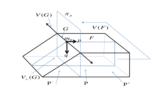
Figure 5. Transitivity.

See Figure 5 that visualizes Proposition 9.1 and Lemma 9.1.

Definition 9.1.

Let $V$ be a subspace of $\mathbb{R}^{n}$. Denote a projection from $\mathbb{R}^{n}$ to $V$ by $P_{V}$.

Lemma 9.1.

Let $\mathbb{P}$ be a polyhedron in $\mathbb{R}^{n}$ and $\mathbb{G}\preceq\mathbb{P}$. Given $\mathfrak{q}\in(\mathbb{G}^{*})^{\circ}|\mathbb{P}$, there exists $r>0$ depending only $\mathfrak{q}$ such that for any $\mathfrak{n}\in\mathbb{P}\setminus\mathbb{G}$ and $\mathfrak{m}\in\mathbb{G}$,

(9.1) $$\mathfrak{q}\cdot\frac{{\rm P}_{V^{\perp}(\mathbb{G})}(\mathfrak{n}-\mathfrak{m})}{|{\rm P}_{V^{\perp}(\mathbb{G})}(\mathfrak{n}-\mathfrak{m})|}\geq r>0.$$

Proof.

We start with the case that $\mathbb{G}=\{\mathfrak{m}_{0}\}$ is a vertex of $\mathbb{P}$. Observe that given a polyhedron $\mathbb{Q}$, there exists a small positive number $\epsilon$ such that

$$\left\{\frac{\mathfrak{n}}{|\mathfrak{n}|}:\mathfrak{n}\in\mathbb{Q}\setminus\{0\}\ \text{where $0$ is a vertex of $\mathbb{Q}$}\right\}=\left\{\frac{\mathfrak{n}}{|\mathfrak{n}|}:\mathfrak{n}\in\mathbb{Q},|\mathfrak{n}|\geq\epsilon\right\},$$

which is a closed set in the sphere $\mathbb{S}^{n-1}$. By this, we set a closed set in $\mathbb{S}^{n-1}$:

(9.2) $$S(\mathbb{P}-\mathfrak{m}_{0})=\left\{\frac{\mathfrak{n}-\mathfrak{m}_{0}}{|\mathfrak{n}-\mathfrak{m}_{0}|}:\mathfrak{n}\in\mathbb{P}\setminus\{\mathfrak{m}_{0}\}\right\}.$$

By $\mathfrak{q}\in(\mathbb{G}^{*})^{\circ}|\mathbb{P}$, we have for all $\mathfrak{n}\in\mathbb{P}\setminus\{\mathfrak{m}_{0}\},$

$$\mathfrak{q}\cdot\frac{\mathfrak{n}-\mathfrak{m}_{0}}{|\mathfrak{n}-\mathfrak{m}_{0}|}>0,\ \text{which with (\ref{s0}) implies that}\ \ \mathfrak{q}\cdot\mathfrak{s}>0\ \text{for}\ \mathfrak{s}\in S(\mathbb{P}-\mathfrak{m}_{0}).$$

A map $\mathfrak{s}\rightarrow\mathfrak{q}\cdot\mathfrak{s}$ is continuous on the compact set $S(\mathbb{P}-\mathfrak{m}_{0})$. So it has a minimum $r>0$:

(9.3) $$\mathfrak{q}\cdot\mathfrak{s}\geq r\ \text{for all}\ \ \mathfrak{s}\in S(\mathbb{P}-\mathfrak{m}_{0}).$$

From $V(\mathbb{G})=\{0\}$ and $V^{\perp}(\mathbb{G})=\mathbb{R}^{n}$,

$${\rm P}_{V^{\perp}(\mathbb{G})}(\mathfrak{n}-\mathfrak{m}_{0})=\mathfrak{n}-\mathfrak{m}_{0}.$$

From this together with (9.2),

$$S(\mathbb{P}-\mathfrak{m}_{0})=\left\{\frac{{\rm P}_{V^{\perp}(\mathbb{G})}(\mathfrak{n}-\mathfrak{m}_{0})}{|{\rm P}_{V^{\perp}(\mathbb{G})}(\mathfrak{n}-\mathfrak{m}_{0})|}:\mathfrak{n}\in\mathbb{P}\setminus\{\mathfrak{m}_{0}\}\right\}.$$

By this and (9.3),

$$\mathfrak{q}\cdot\frac{{\rm P}_{V^{\perp}(\mathbb{G})}(\mathfrak{n}-\mathfrak{m}_{0})}{|{\rm P}_{V^{\perp}(\mathbb{G})}(\mathfrak{n}-\mathfrak{m}_{0})|}\geq r\ \text{for all}\ \ \mathfrak{n}\in\mathbb{P}\setminus\{\mathfrak{m}_{0}\}.$$

We next consider the general case that $\mathbb{G}$ is a $k$-dimensional face of $\mathbb{P}$. We shall use the following two properties:

(9.4) $$\left\{{\bf x}:\rm{P}_{V^{\perp}(\mathbb{G})}({\bf x})=0\right\}=V(\mathbb{G})$$

and

(9.5) $$\ \text{If $\mathfrak{n}\in\mathbb{P}\setminus\mathbb{G}$ and $\mathfrak{m}\in\mathbb{G}$,\ then}\ \ \mathfrak{n}-\mathfrak{m}\notin V(\mathbb{G}).$$

Choose any $\mathfrak{m}_{0}\in\mathbb{G}\preceq\mathbb{P}$. Since an image of polyhedron under any linear transform is also a polyhedron, we see that $\rm{P}_{V^{\perp}(\mathbb{G})}(\mathbb{P}-\mathfrak{m}_{0})$ is a polyhedron in $V^{\perp}(\mathbb{G})$. Moreover,

(9.6) $0$ is a vertex of $\rm{P}_{V^{\perp}(\mathbb{G})}(\mathbb{P}-\mathfrak{m}_{0})$.

Proof of (9.6).

By Definition 2.10, we see that for $\mathfrak{q}\in(\mathbb{G}^{*})^{\circ}|\mathbb{P}$ and for $\mathfrak{m}\in\mathbb{G}$ and $\mathfrak{n}\in\mathbb{P}\setminus\mathbb{G}$,

(9.7) $$0<\mathfrak{q}\cdot(\mathfrak{n}-\mathfrak{m}).$$

Let $\rm{P}_{V^{\perp}(\mathbb{G})}(\mathfrak{n}-\mathfrak{m}_{0})\in\rm{P}_{V^{\perp}(\mathbb{G})}(\mathbb{P}-\mathfrak{m}_{0})\setminus\{0\}$, that is, $\rm{P}_{V^{\perp}(\mathbb{G})}(\mathfrak{n}-\mathfrak{m}_{0})\neq 0$. Then we have $\mathfrak{n}-\mathfrak{m}_{0}\notin V(\mathbb{G})$ by (9.4), that is, $\mathfrak{n}\notin\mathbb{G}$. Thus $\mathfrak{n}\in\mathbb{P}\setminus\mathbb{G}$. By (9.7),

$$\mathfrak{q}\cdot 0=0<\mathfrak{q}\cdot(\mathfrak{n}-\mathfrak{m})=\mathfrak{q}\cdot(\mathfrak{n}-\mathfrak{m}_{0})=\mathfrak{q}\cdot\rm{P}_{V^{\perp}(\mathbb{G})}(\mathfrak{n}-\mathfrak{m}_{0})$$

where $\mathfrak{q}\perp V(\mathbb{G})$ in the last equality. Thus the condition (2.3) of Definition 2.7 holds. ∎

In view of (9.2) and (9.6), we set a compact set

(9.8) $$K=S(\rm{P}_{V^{\perp}(\mathbb{G})}(\mathbb{P}-\mathfrak{m}_{0})-0)=\left\{\frac{\mathfrak{n}-0}{|\mathfrak{n}-0|}:\mathfrak{n}\in\rm{P}_{V^{\perp}(\mathbb{G})}(\mathbb{P}-\mathfrak{m}_{0})\setminus\{0\}\right\}.$$

In the above,

(9.9) $$\rm{P}_{V^{\perp}(\mathbb{G})}(\mathbb{P}-\mathfrak{m}_{0})\setminus\{0\}=\rm{P}_{V^{\perp}(\mathbb{G})}((\mathbb{P}\setminus\mathbb{G})-\mathbb{G}),$$

Proof of (9.9).

Let ${\bf z}\in\rm{P}_{V^{\perp}(\mathbb{G})}(\mathbb{P}-\mathfrak{m}_{0})\setminus\{0\}$. Then ${\bf z}=\rm{P}_{V^{\perp}(\mathbb{G})}(\mathfrak{n}-\mathfrak{m}_{0})\neq 0$ with $\mathfrak{n}\in\mathbb{P}$. From (9.4) $\mathfrak{n}-\mathfrak{m}_{0}\notin V(\mathbb{G})$, which also implies that $\mathfrak{n}\notin\mathbb{G}$. Thus ${\bf z}\in\rm{P}_{V^{\perp}(\mathbb{G})}((\mathbb{P}\setminus\mathbb{G})-\mathbb{G})$.
Let ${\bf z}\in\rm{P}_{V^{\perp}(\mathbb{G})}((\mathbb{P}\setminus\mathbb{G})-\mathbb{G})$. Then ${\bf z}=\rm{P}_{V^{\perp}(\mathbb{G})}(\mathfrak{n}-\mathfrak{m})$ with $\mathfrak{n}\in\mathbb{P}\setminus\mathbb{G}$ and $\mathfrak{m}\in\mathbb{G}$. Thus

$${\bf z} = \rm{P}_{V^{\perp}(\mathbb{G})}(\mathfrak{n}-\mathfrak{m}_{0}+\mathfrak{m}_{0}-\mathfrak{m})$$

$$= \rm{P}_{V^{\perp}(\mathbb{G})}(\mathfrak{n}-\mathfrak{m}_{0})+\rm{P}_{V^{\perp}(\mathbb{G})}(\mathfrak{m}_{0}-\mathfrak{m})$$

$$= \rm{P}_{V^{\perp}(\mathbb{G})}(\mathfrak{n}-\mathfrak{m}_{0})\neq 0$$

where the last inequality follows from (9.4) and (9.5). Hence ${\bf z}\in\rm{P}_{V^{\perp}(\mathbb{G})}(\mathbb{P}-\mathfrak{m}_{0})\setminus\{0\}$. ∎

By (9.9), we rewrite the compact set in (9.8) as

(9.10) $$K=\left\{\frac{\rm{P}_{V^{\perp}(\mathbb{G})}(\mathfrak{n}-\mathfrak{m})}{|\rm{P}_{V^{\perp}(\mathbb{G})}(\mathfrak{n}-\mathfrak{m})|}:\mathfrak{n}\in\mathbb{P}\setminus\mathbb{G},\mathfrak{m}\in\mathbb{G}\right\}.$$

By $\mathfrak{q}\in(\mathbb{G}^{*})^{\circ}|\mathbb{P}$, for all $\mathfrak{n}\in\mathbb{P}\setminus\mathbb{G}$ and $\mathfrak{m}\in\mathbb{G}$,

$$\mathfrak{q}\cdot\rm{P}_{V^{\perp}(\mathbb{G})}(\mathfrak{n}-\mathfrak{m})=\mathfrak{q}\cdot(\mathfrak{n}-\mathfrak{m})>0$$

because of $\mathfrak{q}\perp V(\mathbb{G})$ and Definition 2.10. Therefore

$$\mathfrak{q}\cdot\mathfrak{s}>0\ \text{for $\mathfrak{s}\in K$.}$$

From this combined with the compactness of $K$, there exists $r>0$ such that

$$\mathfrak{q}\cdot\mathfrak{s}\geq r\ \text{for all $\mathfrak{s}\in K$.}$$

By (9.10), for any $\mathfrak{n}\in\mathbb{P}\setminus\mathbb{G}$ and $\mathfrak{m}\in\mathbb{G}$,

$$\mathfrak{q}\cdot\frac{{\rm P}_{V^{\perp}(\mathbb{G})}(\mathfrak{n}-\mathfrak{m})}{|{\rm P}_{V^{\perp}(\mathbb{G})}(\mathfrak{n}-\mathfrak{m})|}\geq r>0.$$

This completes the proof of Lemma 9.1. ∎

Proof of Proposition 9.1.

It suffices to show that $0<\epsilon<\epsilon_{0}$ implies that for all $\mathfrak{n}\in\mathbb{P}\setminus\mathbb{G}$ and $\mathfrak{m}\in\mathbb{G}$,

(9.11) $$(\mathfrak{q}+\epsilon\mathfrak{p})\cdot(\mathfrak{n}-\mathfrak{m})>0.$$

We first observe from $\mathfrak{q}\in(\mathbb{F}^{*})^{\circ}|\mathbb{P}$,

(9.12) $$\mathfrak{q}\cdot(\mathfrak{n}-\mathfrak{m})\geq 0\ \ \text{for all $\mathfrak{n}\in\mathbb{P}\setminus\mathbb{G}$ and $\mathfrak{m}\in\mathbb{G}$}.$$

Moreover, combined with $\mathfrak{p}\in(\mathbb{G}^{*})^{\circ}|\mathbb{F}$,

(9.13) $$\mathfrak{q}\cdot(\mathfrak{n}-\mathfrak{m})>0\ \ \text{for all $\mathfrak{n}\in\mathbb{P}\setminus\mathbb{F}$ and $\mathfrak{m}\in\mathbb{G}$},$$

(9.14) $$\mathfrak{p}\cdot(\mathfrak{n}-\mathfrak{m})>0\ \ \text{for all $\mathfrak{n}\in\mathbb{F}\setminus\mathbb{G}$ and $\mathfrak{m}\in\mathbb{G}$}$$

Let $\pi_{\mathfrak{p}}$ be a supporting plane of $\mathbb{G}\preceq\mathbb{F}$,

$$\mathbb{G}\subset\pi_{\mathfrak{p}}\ \ \text{and}\ \ \mathbb{F}\setminus\mathbb{G}\subset(\pi_{\mathfrak{p}}^{+})^{\circ}.$$

Split

$$\mathbb{P}=\left(\mathbb{P}\cap\pi_{\mathfrak{p}}^{-}\right)\cup\left(\mathbb{P}\cap\pi_{\mathfrak{p}}^{+}\right)=\mathbb{P}^{-}\cup\mathbb{P}^{+}\ \text{that are visualized in Figure \ref{graph4}}.$$

Case 1. Suppose $\mathfrak{n}\in\mathbb{P}^{+}\setminus\mathbb{G}$. Then in view that $\mathfrak{n}\in\mathbb{P}^{+}\subset\pi_{\mathfrak{p}}^{+}$,

(9.15) $$\mathfrak{p}\cdot(\mathfrak{n}-\mathfrak{m})\geq 0\ \ \text{for all $\mathfrak{n}\in\mathbb{P}\setminus\mathbb{G}$ and $\mathfrak{m}\in\mathbb{G}$}.$$

By (9.12) and (9.15), we have $\geq$ in (9.11). Thus either (9.13) or (9.14) yields $>$ in (9.11).
Case 2. Suppose that $\mathfrak{n}\in\mathbb{P}^{-}\setminus\mathbb{G}$. Note that $\mathbb{G}\preceq\mathbb{P}^{-}$. Consider a hyperplane $\pi_{\mathfrak{q}}(\mathbb{F})$ containing $\mathbb{F}$ and whose normal vector is $\mathfrak{q}$. Then $\pi_{\mathfrak{q}}(\mathbb{F})$ is a supporting plane of $\mathbb{G}\preceq\mathbb{P}^{-}$. Thus

$$\mathfrak{q}\in(\mathbb{G}^{*})^{\circ}|(\mathbb{P}^{-},\mathbb{R}^{n}).$$

Hence by Lemma 9.1, for all $\mathfrak{n}\in\mathbb{P}^{-}\setminus\mathbb{G}$ and $\mathfrak{m}\in\mathbb{G}$,

(9.16) $$\mathfrak{q}\cdot\frac{{\rm P}_{V^{\perp}(\mathbb{G})}(\mathfrak{n}-\mathfrak{m})}{|{\rm P}_{V^{\perp}(\mathbb{G})}(\mathfrak{n}-\mathfrak{m})|}\geq r>0\ \ \text{and}\ \ {\rm P}_{V^{\perp}(\mathbb{G})}(\mathfrak{n}-\mathfrak{m})\neq 0$$

where the last follows from (9.4) and (9.5). Split

$$\mathfrak{n}-\mathfrak{m}={\rm P}_{V(\mathbb{G})}(\mathfrak{n}-\mathfrak{m})+{\rm P}_{V^{\perp}(\mathbb{G})}(\mathfrak{n}-\mathfrak{m}).$$

Since $\mathfrak{q}\in(\mathbb{G}^{*})^{\circ}|(\mathbb{P}^{-},\mathbb{R}^{n})$ and $\mathfrak{p}\in(\mathbb{G}^{*})^{\circ}|\mathbb{F}$, that is $\mathfrak{q},\mathfrak{p}\perp V(\mathbb{G})$,

$$\mathfrak{q}\cdot{\rm P}_{V(\mathbb{G})}(\mathfrak{n}-\mathfrak{m})=\mathfrak{p}\cdot{\rm P}_{V(\mathbb{G})}(\mathfrak{n}-\mathfrak{m})=0.$$

So

$$(\mathfrak{q}+\epsilon\mathfrak{p})\cdot(\mathfrak{n}-\mathfrak{m})=(\mathfrak{q}+\epsilon\mathfrak{p})\cdot{\rm P}_{V^{\perp}(\mathbb{G})}(\mathfrak{n}-\mathfrak{m}).$$

Choose $\epsilon_{0}=\frac{r}{100|\mathfrak{p}|}$ and $0<\epsilon<\epsilon_{0}$. Then, by (9.16),

$$(\mathfrak{q}+\epsilon\mathfrak{p})\cdot(\mathfrak{n}-\mathfrak{m}) = (\mathfrak{q}+\epsilon\mathfrak{p})\cdot{\rm P}_{V^{\perp}(\mathbb{G})}(\mathfrak{n}-\mathfrak{m})$$

$$\geq r\left|{\rm P}_{V^{\perp}(\mathbb{G})}(\mathfrak{n}-\mathfrak{m})\right|-\epsilon|\mathfrak{p}|\left|{\rm P}_{V^{\perp}(\mathbb{G})}(\mathfrak{n}-\mathfrak{m})\right|$$

$$\geq \frac{99}{100}r\left|{\rm P}_{V^{\perp}(\mathbb{G})}(\mathfrak{n}-\mathfrak{m})\right|>0.$$

This completes the proof of Proposition 9.1 ∎

Lemma 9.2.

Let $\mathbb{P}_{\nu}\subset\mathbb{R}^{n}$ be a polyhedron and $\mathbb{F}_{\nu},\mathbb{G}_{\nu}\in\mathcal{F}(\mathbb{P}_{\nu})$ such that $\mathbb{G}_{\nu}\preceq\mathbb{F}_{\nu}$. Suppose that $\mathfrak{q}\in\bigcap_{\nu}(\mathbb{F}_{\nu}^{*})^{\circ}|(\mathbb{P}_{\nu},\mathbb{R}^{n})$. Suppose $\mathfrak{p}\in\bigcap_{\nu}(\mathbb{G}_{\nu}^{*})^{\circ}|(\mathbb{F}_{\nu},\mathbb{R}^{n})$. Then there exists a vector ${\bf w}\in\bigcap(\mathbb{G}_{\nu}^{*})^{\circ}|(\mathbb{P}_{\nu},\mathbb{R}^{n})$.

Proof.

By Proposition 9.1, there exists $\epsilon_{\nu}>0$ such that for $0<\epsilon<\epsilon_{\nu}$, $\mathfrak{q}+\epsilon\mathfrak{p}\in(\mathbb{G_{\nu}}^{*})^{\circ}|(\mathbb{P}_{\nu},\mathbb{R}^{n}).$ Choose $\epsilon_{0}=\min\{\epsilon_{\nu}:\nu=1,\cdots,d\}$. Then for $0<\epsilon<\epsilon_{0}$, $\mathfrak{q}+\epsilon\mathfrak{p}\in\bigcap_{\nu=1}^{d}(\mathbb{G_{\nu}}^{*})^{\circ}|(\mathbb{P}_{\nu},\mathbb{R}^{n}).$ ∎

9.2. Lemma for Necessity

Lemma 9.3.

Let $\Lambda=(\Lambda_{\nu})$ with $\Lambda_{\nu}\subset\mathbb{Z}_{+}^{n}$ and let $P_{\Lambda}\in\mathcal{P}_{\Lambda}$. Fix $S\subset\{1,\cdots,n\}$. Given $\mathbb{F}=(\mathbb{F}_{\nu})\in\mathcal{F}({\bf N}(\Lambda,S))$, define

$$\mathcal{I}(P_{\mathbb{F}},\xi,r) = \int_{\prod(-r_{j},r_{j})}e^{i\left(\xi_{1}\sum_{\mathfrak{m}\in\mathbb{F}_{1}\cap\Lambda_{1}}c_{\mathfrak{m}}^{1}t^{\mathfrak{m}}+\cdots+\xi_{d}\sum_{\mathfrak{m}\in\mathbb{F}_{d}\cap\Lambda_{d}}c_{\mathfrak{m}}^{d}t^{\mathfrak{m}}\right)}\frac{dt_{1}}{t_{1}}\cdots\frac{dt_{n}}{t_{n}},$$

$$\mathcal{I}(P_{\mathbb{F}},\xi,a,b) = \int_{\prod\{a_{j}<|t_{j}|<b_{j}\}}e^{i\left(\xi_{1}\sum_{\mathfrak{m}\in\mathbb{F}_{1}\cap\Lambda_{1}}c_{\mathfrak{m}}^{1}t^{\mathfrak{m}}+\cdots+\xi_{d}\sum_{\mathfrak{m}\in\mathbb{F}_{d}\cap\Lambda_{d}}c_{\mathfrak{m}}^{d}t^{\mathfrak{m}}\right)}\frac{dt_{1}}{t_{1}}\cdots\frac{dt_{n}}{t_{n}}.$$

Suppose that

$$\sup_{r\in I(S),\xi\in\mathbb{R}^{d}}\left|\mathcal{I}(P_{\Lambda},\xi,r)\right|<\infty$$

where $I(S)$ is as defined in (1.3). Suppose also that

$${\bf u}=(u_{1},\cdots,u_{n})\in\bigcap_{\nu=1}^{d}(\mathbb{F}_{\nu}^{*})^{\circ}\neq\emptyset$$

where

(9.17) $$\text{ $u_{j}>0$ for $j\in S\setminus S_{0}$ and $u_{j}=0$ for $j\in S_{0}\subset S$ by Lemma \ref{lem132}}.$$

Then

(9.18) $$\sup_{\xi\in\mathbb{R}^{d},a,b\in I(S_{0})}\left|\mathcal{I}(P_{\mathbb{F}},\xi,a,b)\right| < \infty.$$

Proof of (9.18).

By the definition of $(\mathbb{F}_{\nu}^{*})^{\circ}$, there exists $\rho_{\nu}$ such that

(9.19) $${\bf u}\cdot\mathfrak{m}=\rho_{\nu}<{\bf u}\cdot\mathfrak{n}\ \ \text{for all $\mathfrak{m}\in\mathbb{F}_{\nu}$ and $\mathfrak{n}\in{\bf N}(\Lambda_{\nu},S)\setminus\mathbb{F}_{\nu}$}.$$

Let $a=(a_{j}),b=(b_{j})\in I(S_{0})$ where $I(S_{0})=\prod_{j=1}^{n}I_{j}$ where

(9.20) $$I_{j}=(0,\infty) j\in\{1,\cdots,n\}\setminus S_{0} I_{j}=(0,1) j\in S_{0}$$ for and for as in (1.3).

Let $\rho=(\rho_{\nu})$ with $\rho_{\nu}$ in (9.19). Set

$$I(a(\delta),b(\delta))=\prod_{j=1}^{n}\{a_{j}\delta^{u_{j}}<|t_{j}|<b_{j}\delta^{u_{j}}\}\ \ \text{and}\ \ \delta^{-\rho}\xi=(\delta^{-\rho_{1}}\xi_{1},\cdots,\delta^{-\rho_{d}}\xi_{d}).$$

Then

$$\mathcal{I}(P_{\Lambda},\delta^{-\rho}\xi,a(\delta),b(\delta))$$

$$\qquad\qquad=\int_{I(a(\delta),b(\delta))}e^{i\left(\delta^{-\rho_{1}}\xi_{1}\sum_{\mathfrak{m}\in\Lambda_{1}}c_{\mathfrak{m}}^{1}t^{\mathfrak{m}}+\cdots+\delta^{-\rho_{d}}\xi_{d}\sum_{\mathfrak{m}\in\Lambda_{d}}c_{\mathfrak{m}}^{d}t^{\mathfrak{m}}\right)}\frac{dt_{1}}{t_{1}}\cdots\frac{dt_{n}}{t_{n}}.$$

By (9.17) and (9.20), we find a sufficiently small $\delta$ such that

$$\delta^{u_{j}}a_{j},\delta^{u_{j}}b_{j}<1\ \ \text{for $j\in S\setminus S_{0}$\ \ and \ }\delta^{u_{j}}a_{j}=a_{j},\delta^{u_{j}}b_{j}=b_{j}<1\ \ \text{ for $j\in S_{0}\subset S$. }$$

Thus $a(\delta),b(\delta)\in I(S)$. Hence, by our hypothesis

(9.21) $$\left|\mathcal{I}(P_{\Lambda},\delta^{-\rho}\xi,a(\delta),b(\delta))\right|\leq C\ \text{uniformly in $\xi$ and $a,b,\delta$.}$$

Consider the difference of two multipliers given by

$$M(\xi,\delta,a,b) = \mathcal{I}(P_{\Lambda},\delta^{-\rho}\xi,a(\delta),b(\delta))-\mathcal{I}(P_{\mathbb{F}},\delta^{-\rho}\xi,a(\delta),b(\delta))$$

$$= \int_{I(a(\delta),b(\delta))}e^{i\left(\xi_{1}\delta^{-\rho_{1}}\sum_{\mathfrak{m}\in\Lambda_{1}}c_{\mathfrak{m}}^{1}t^{\mathfrak{m}}+\cdots+\xi_{d}\delta^{-\rho_{d}}\sum_{\mathfrak{m}\in\Lambda_{d}}c_{\mathfrak{m}}^{d}t^{\mathfrak{m}}\right)}\frac{dt_{1}}{t_{1}}\cdots\frac{dt_{n}}{t_{n}}$$

$$- \int_{I(a(\delta),b(\delta))}e^{i\left(\xi_{1}\delta^{-\rho_{1}}\sum_{\mathfrak{m}\in\mathbb{F}_{1}\cap\Lambda_{1}}c_{\mathfrak{m}}^{1}t^{\mathfrak{m}}+\cdots+\xi_{d}\delta^{-\rho_{d}}\sum_{\mathfrak{m}\in\mathbb{F}_{d}\cap\Lambda_{d}}c_{\mathfrak{m}}^{d}t^{\mathfrak{m}}\right)}\frac{dt_{1}}{t_{1}}\cdots\frac{dt_{n}}{t_{n}}.$$

By the mean value theorem and change of variable $t_{j}^{\prime}=\delta^{-u_{j}}t_{j}$ in the above two integrals,

$$|M(\xi,\delta,a,b)|$$

$$\quad\leq\int_{I(a,b)}\left|\xi_{1}\sum_{\mathfrak{n}\in\Lambda_{1}\setminus\mathbb{F}_{1}}\delta^{{\bf u}\cdot\mathfrak{n}-\rho_{1}}c_{\mathfrak{n}}^{1}t^{\mathfrak{n}}+\cdots+\xi_{d}\sum_{\mathfrak{n}\in\Lambda_{d}\setminus\mathbb{F}_{d}}\delta^{{\bf u}\cdot\mathfrak{n}-\rho_{d}}c_{\mathfrak{n}}^{d}t^{\mathfrak{n}}\right|\frac{dt_{1}}{|t_{1}|}\cdots\frac{dt_{n}}{|t_{n}|}$$

$$\quad\leq|\xi_{1}|\sum_{\mathfrak{n}\in\Lambda_{1}\setminus\mathbb{F}_{1}}\delta^{{\bf u}\cdot\mathfrak{n}-\rho_{1}}|c_{\mathfrak{n}}^{1}|C^{1}_{\mathfrak{n}}(a,b)+\cdots+|\xi_{d}|\sum_{\mathfrak{n}\in\Lambda_{d}\setminus\mathbb{F}_{d}}\delta^{{\bf u}\cdot\mathfrak{n}-\rho_{d}}|c_{\mathfrak{n}}^{d}|C^{d}_{\mathfrak{n}}(a,b).$$

The constants $C^{1}_{\mathfrak{m}}(a,b),\cdots,C^{d}_{\mathfrak{m}}(a,b)$ above are absolute value for the integral of $\frac{t^{\mathfrak{m}}}{|t_{1}|\cdots|t_{n}|}$ on the region $I(a,b)$. From ${\bf u}\cdot\mathfrak{n}-\rho_{\nu}>0$ in (9.19), we can choose $\delta>0$ so that $\delta^{{\bf u}\cdot\mathfrak{n}-\rho_{\nu}}$ above is small enough to satisfy

$$|M(\xi,\delta,a,b)| \leq 1.$$

By this and (9.21),

(9.22) $$\left|\mathcal{I}(P_{\mathbb{F}},\delta^{-\rho}\xi,a(\delta),b(\delta))\right|\leq C.$$

By (9.19) and the change of variables $\delta^{-u_{j}}t_{j}=t_{j}^{\prime}$ for all $j=1,\cdots,n$,

$$\mathcal{I}(P_{\mathbb{F}},\delta^{-\rho}\xi,a(\delta),b(\delta))$$

$$\quad=\int_{I(a(\delta),b(\delta))}e^{i\left(\xi_{1}\delta^{-\rho_{1}}\sum_{\mathfrak{m}\in\mathbb{F}_{1}}c_{\mathfrak{m}}^{1}t^{\mathfrak{m}}+\cdots+\xi_{d}\delta^{-\rho_{d}}\sum_{\mathfrak{m}\in\mathbb{F}_{d}}c_{\mathfrak{m}}^{d}t^{\mathfrak{m}}\right)}\frac{dt_{1}}{t_{1}}\cdots\frac{dt_{n}}{t_{n}}$$

$$\quad=\int_{I(a,b)}e^{i\left(\xi_{1}\sum_{\mathfrak{m}\in\mathbb{F}_{1}}c_{\mathfrak{m}}^{1}t^{\mathfrak{m}}+\cdots+\xi_{d}\sum_{\mathfrak{m}\in\mathbb{F}_{d}}c_{\mathfrak{m}}^{d}t^{\mathfrak{m}}\right)}\frac{dt_{1}}{t_{1}}\cdots\frac{dt_{n}}{t_{n}}=\mathcal{I}(P_{\mathbb{F}},\xi,a,b).$$

Hence this identity combined with (9.22) yields (9.18). ∎

9.3. Necessity Theorem

Definition 9.2.

To each subset $M=\{\mathfrak{q}_{1},\cdots,\mathfrak{q}_{N}\}\subset\mathbb{R}^{n}$, we associate a matrix:

$$\rm{Mtr}(M)=\left(\begin{matrix}&\mathfrak{q}_{1}&\\ &\vdots&\\ &\mathfrak{q}_{N}&\end{matrix}\right)$$

whose rows are vectors in $M$. We define a class of rank $m$-subsets in $\mathbb{R}^{n}$:

(9.23) $$\qquad\ \ \mathcal{M}_{m,n}=\biggl{\{}M\subset\mathbb{R}^{n}:\rm{Mtr}(M)\sim\left(\begin{matrix}1&0&\cdots&0&a_{1,m+1}&\cdots&a_{1,n}\\ 0&1&0&\vdots&a_{2,m+1}&\cdots&a_{2,n}\\ \vdots&0&1&0&\vdots&\cdots&\vdots\\ 0&\cdots&0&1&a_{m,m+1}&\cdots&a_{m,n}\end{matrix}\right)\biggl{\}}.$$

Here $\sim$ means row equivalence and $(a_{ij})_{1\leq i\leq m,\,m+1\leq j\leq n}$ a real $m\times(n-m)$ matrix.

Theorem 9.1 (Necessity Part of Main Theorems 1 through 3).

Let $\Lambda=(\Lambda_{\nu})$ where $\Lambda_{\nu}\subset\mathbb{Z}_{+}^{n}$ is a finite set for $\nu=1,\cdots,d$ and let $S\subset\{1,\cdots,n\}$. Suppose that there exist faces $\mathbb{F}\in\mathcal{F}({\bf N}(\Lambda,S))$ such that

(9.24) $$\bigcup_{\nu=1}^{d}\left(\mathbb{F}_{\nu}\cap\Lambda_{\nu}\right)\ \text{ is not an even set\,, }$$

and $\mathbb{F}\in\mathcal{F}_{\rm{lo}}({\bf N}(\Lambda,S))$, that is,

(9.25) $$\text{rank}\left(\bigcup_{\nu}\mathbb{F}_{\nu}\right)\leq n-1\ \ \text{and}\ \ \bigcap_{\nu}(\mathbb{F}_{\nu}^{*})^{\circ}|{\bf N}(\Lambda_{\nu},S)\neq\emptyset.$$

Then there exist a vector polynomial $P_{\Lambda}\in\mathcal{P}_{\Lambda}$ so that

$$\sup_{\xi\in\mathbb{R}^{d},r\in I(S)}\left|\mathcal{I}(P_{\Lambda},\xi,r)\right|=\infty.$$

Proof of Theorem 9.1.

Choose the integer $m$ such that

(9.26) $$m=\min\left\{\text{rank}\big{(}\bigcup_{\nu}\mathbb{F}_{\nu}\big{)}:\exists\ \mathbb{F}\in\mathcal{F}({\bf N}(\Lambda,S))\ \text{satisfying (\ref{912}), (\ref{913})}\right\}.$$

Then we have $\mathbb{F}=(\mathbb{F}_{\nu})$ with $\mathbb{F}_{\nu}\in\mathcal{F}({\bf N}(\Lambda_{\nu},S))$ such that

(9.27) $$\bigcup_{\nu=1}^{d}\left(\mathbb{F}_{\nu}\cap\Lambda_{\nu}\right)\ \text{ is not an even set\,, }$$

and

(9.28) $$\text{rank}\left(\bigcup_{\nu}\mathbb{F}_{\nu}\right)=m\leq n-1\ \ \text{and}\ \ \bigcap_{\nu}(\mathbb{F}_{\nu}^{*})^{\circ}|{\bf N}(\Lambda_{\nu},S)\neq\emptyset.$$

This with (9.23) implies that we can assume that without loss of generality,

(9.29) $$\text{Sp}\left(\bigcup_{\nu}\mathbb{F}_{\nu}\right)\in\mathcal{M}_{m,n}.$$

By (9.28) and (9.17), we have for some $S_{0}\subset S\subset N_{n}$

$$(u_{j})\in\bigcap_{\nu}(\mathbb{F}_{\nu}^{*})^{\circ}|{\bf N}(\Lambda_{\nu},S)\ \ \text{and}\ \ u_{j}=0\ \ \text{for $j\in S_{0}$ and $u_{j}>0$ for $j\in S\setminus S_{0}$}.$$

By Lemma 4.7,

(9.30) $$\{{\bf e}_{j}:j\in S_{0}\}\subset\text{Sp}\left(\bigcup_{\nu}\mathbb{F}_{\nu}\right).$$

Moreover by (9.26), for any $\mathbb{G}_{\nu}\preceq\mathbb{F}_{\nu}$,

(9.31) $$\bigcup\mathbb{G}_{\nu}\cap\Lambda_{\nu}\ \ \text{is even }\ \text{whenever}\ \text{rank}\,\big{(}\bigcup\mathbb{G}_{\nu}\big{)}\leq m-1\ \text{and}\ \bigcap(\mathbb{G}_{\nu}^{*})^{\circ}|{\bf N}(\Lambda_{\nu},S)\neq\emptyset.$$

In order to show Theorem 9.1, by Lemma 9.3, it suffices to find, under the assumption (9.27)-(9.31), a polynomial $P_{\Lambda}(t)=\left(\sum_{\mathfrak{q}\in\Lambda_{\nu}}c^{\nu}_{\mathfrak{q}}t^{\mathfrak{q}}\right)\in\mathcal{P}_{\Lambda}$ with an appropriate $c^{\nu}_{\mathfrak{q}}$ such that

(9.32) $$\sup_{\xi\in\mathbb{R}^{d},a,b\in I(S_{0})}\left|\mathcal{I}(P_{\mathbb{F}},\xi,a,b)\right| = \infty$$

where

$$\mathcal{I}(P_{\mathbb{F}},\xi,a,b)=\int_{\prod\{a_{j}<|t_{j}|<b_{j}\}}e^{i\left(\xi_{1}\sum_{\mathfrak{m}\in\mathbb{F}_{1}\cap\Lambda_{1}}c_{\mathfrak{m}}^{1}t^{\mathfrak{m}}+\cdots+\xi_{d}\sum_{\mathfrak{m}\in\mathbb{F}_{d}\cap\Lambda_{d}}c_{\mathfrak{m}}^{d}t^{\mathfrak{m}}\right)}\frac{dt_{1}}{t_{1}}\cdots\frac{dt_{n}}{t_{n}}.$$

Definition 9.3.

Let $1\leq m<n$. Using $\mathbb{R}^{n}=X\bigoplus Y$ with $X=\mathbb{R}^{m}\times\{0\}$ and $Y=\{0\}\times\mathbb{R}^{n-m}$, we write $a=(a_{1},\cdots,a_{n})\in\mathbb{R}^{n}$ as $a=(a_{X},a_{Y})$ so that

$$a_{X}=(a_{1},\cdots,a_{m})\in\mathbb{R}^{m}\ \ \text{and}\ \ a_{Y}=(a_{m+1},\cdots,a_{n})\in\mathbb{R}^{n-m}.$$

Note that $1_{X}(S_{0})$ is restricted to $\mathbb{R}^{m}$ so that

$$1_{X}(S_{0})=(r_{j})_{j=1}^{m} r_{j}=1 j\in S_{0} r_{j}=\infty j\in N_{m}\setminus S_{0}$$ with for and for  ,

and $I_{X}(S_{0})$ is also restricted to $\mathbb{R}^{m}$ in view of (1.3) so that

$$\qquad I_{X}(S_{0})=\prod_{j=1}^{m}I_{j}\ \text{ where $I_{j}=(0,1)$ for $j\in S_{0}$ and $I_{j}=(0,\infty)$ for $j\in N_{m}\setminus S_{0}$. }$$

To show (9.32), we prove that there exists $C(\xi)>0$,

(9.33) $$\left|\lim_{a_{X}\rightarrow 0,b_{X}\rightarrow 1_{X}(S_{0})}\mathcal{I}(P_{\mathbb{F}},\xi,a,b)\right|\geq C(\xi)\prod_{j=m+1}^{n}\log(b_{j}/a_{j})\rightarrow\infty\ \ \text{as}\ a_{j}\rightarrow 0\,,$$

where the integral $\mathcal{I}(P_{\mathbb{F}},\xi,a,b)$ is evaluated so that $\frac{dt_{1}}{t_{1}}\cdots\frac{dt_{m}}{t_{m}}$ first and $\frac{dt_{m+1}}{t_{m+1}}\cdots\frac{dt_{n}}{t_{n}}$ next:

$$\mathcal{I}(P_{\mathbb{F}},\xi,a,b)=\int_{\prod_{j=m+1}^{n}\{a_{j}<|t_{j}|<b_{j}\}}\left[\int_{\prod_{j=1}^{m}\{a_{j}<|t_{j}|<b_{j}\}}e^{i\xi\cdot P_{\mathbb{F}}(t)}\frac{dt_{1}}{t_{1}}\cdots\frac{dt_{m}}{t_{m}}\right]\frac{dt_{m+1}}{t_{m+1}}\cdots\frac{dt_{n}}{t_{n}}.$$

As a first step to show (9.33), we write the integral in (9.33) as

(9.34) $$\int_{\prod_{j=m+1}^{n}\{a_{j}<|t_{j}|<b_{j}\}}\left[\lim_{a_{X}\rightarrow 0,b_{X}\rightarrow 1_{X}(S_{0})}\int_{\prod_{j=1}^{m}\{a_{j}<|t_{j}|<b_{j}\}}e^{i\xi\cdot P_{\mathbb{F}}(t)}\frac{dt_{1}}{t_{1}}\cdots\frac{dt_{m}}{t_{m}}\right]\frac{dt_{m+1}}{t_{m+1}}\cdots\frac{dt_{n}}{t_{n}}.$$

This follows from the dominated convergence theorem. To apply the convergence theorem, we shall prove that for each $t_{Y}=(t_{m+1},\cdots,t_{n})\in\prod_{j=m+1}^{n}\{a_{j}<|t_{j}|<b_{j}\}$

(9.35) $$\sup_{\xi\in\mathbb{R}^{d},a_{X},b_{X}\in I_{X}(S_{0})}\left|\int_{\prod_{j=1}^{m}\{a_{j}<|t_{j}|<b_{j}\}}e^{i\xi\cdot P_{\mathbb{F}}(t)}\frac{dt_{1}}{t_{1}}\cdots\frac{dt_{m}}{t_{m}}\right|\leq C((a_{j})_{j=m+1}^{n},(b_{j})_{j=m+1}^{n}),$$

and that

(9.36) $$\lim_{a_{X}\rightarrow 0,b_{X}\rightarrow 1_{X}(S_{0})}\int_{\prod_{j=1}^{m}\{a_{j}<|t_{j}|<b_{j}\}}e^{i\xi\cdot P_{\mathbb{F}}(t)}\frac{dt_{1}}{t_{1}}\cdots\frac{dt_{m}}{t_{m}}\ \text{exists}.$$

Assume that (9.35) and (9.36) are proved in the next section. Then, by writing each integral in the $n$-tuple integral (9.34) as the sum of 2 integrals by separating the variables into the positive and negative parts, we decompose the above $n$-tuple integral into the sum of $2^{n}$ pieces. For this purpose, we denote $\,O=\{\sigma=(\sigma_{j})=(\underbrace{\pm 1,\cdots,\pm 1}_{\text{$n$ components}})\}\,,$ the sign-index set of $2^{n}$ elements. Next by using the change of variables $\,t_{1}=\sigma_{1}t_{1}^{\prime},\cdots,\,t_{n}^{\prime}=\sigma_{n}t_{n}^{\prime}\,$ in each integration, we write the integral (9.34) as

(9.37) $$\int_{\prod_{j=m+1}^{n}\{a_{j}<t_{j}<b_{j}\}}\mathcal{J}(P_{\mathbb{F}},\xi,(t_{m+1},\cdots,t_{n}))\,\frac{dt_{m+1}}{t_{m+1}}\cdots\frac{dt_{n}}{t_{n}}.$$

Here the integrand above is

$$\mathcal{J}(P_{\mathbb{F}},\xi,(t_{m+1},\cdots,t_{n}))$$

(9.38) $$\quad=\lim_{a_{X}\rightarrow 0,b_{X}\rightarrow 1_{X}(S_{0})}\int_{\prod_{j=1}^{m}\{a_{j}<t_{j}<b_{j}\}}\sum_{\sigma\in O}(-1)^{|\sigma|}\exp\left(iP_{\mathbb{F}}(\xi,\sigma t)\right)\frac{dt_{1}}{t_{1}}\cdots\frac{dt_{m}}{t_{m}}$$

where $|\sigma|$ is a number of $-1$ in the components of $\sigma\in O$ and $P_{\mathbb{F}}(\xi,\sigma t)$ is

$$P_{\mathbb{F}}(\xi,\sigma_{1}t_{1},\cdots,\sigma_{n}t_{n})=\sum_{\nu=1}^{d}\left(\sum_{\mathfrak{q}\in\mathbb{F}_{\nu}}c_{\mathfrak{q}}^{\nu}\sigma^{\mathfrak{q}}t^{\mathfrak{q}}\right)\xi_{\nu}.$$

The limit in (9.3) exists by (9.36). Moreover, $\mathcal{J}(P_{\mathbb{F}},\xi,(t_{m+1},\cdots,t_{n}))$ is finite by (9.35). We shall in the next section prove that it is independent of $t_{Y}=(t_{m+1},\cdots,t_{n})$:

(9.39) $$\mathcal{J}(P_{\mathbb{F}},\xi,(t_{m+1},\cdots,t_{n}))=\mathcal{J}(P_{\mathbb{F}},\xi)$$

and non-vanishing:

(9.40) $$\exists\,\text{ $P_{\Lambda}(t)$ and $\xi$ such that }\ \mathcal{J}(P_{\mathbb{F}},\xi)\neq 0.$$

Therefore (9.33) follows from (9.39) and (9.40) in (9.37). We shall prove (9.35) and (9.36) in the first part of Section 10, and show (9.39) and (9.40) in the last part of Section 10. ∎

10. Proof of Necessity

10.1. Proof of (9.35) and (9.36)

Let $\Omega=(\Omega_{\nu})$ where $\Omega_{\nu}\subset\mathbb{R}^{m}$ is given by

(10.1) $$\Omega_{\nu}=(\mathbb{F}_{\nu}\cap\Lambda_{\nu})_{X}=\{(q_{1},\cdots,q_{m}):(q_{1},\cdots,q_{n})\in\mathbb{F}_{\nu}\cap\Lambda_{\nu}\}.$$

For each $t_{Y}=(t_{m+1},\cdots,t_{n})\in\prod_{j=m+1}^{n}\{a_{j}<|t_{j}|<b_{j}\}$, define

$$\mathcal{I}(P_{\Omega},\xi,a_{X},b_{X},t_{Y})=\int_{\prod_{j=1}^{m}\{a_{j}<|t_{j}|<b_{j}\}}e^{i\xi\cdot P_{\mathbb{F}}(t_{1},\cdots,t_{m},t_{Y})}\frac{dt_{1}}{t_{1}}\cdots\frac{dt_{m}}{t_{m}}.$$

To show (9.35) and (9.36), it suffices to show that for all $P_{\Omega}\in\mathcal{P}_{\Omega}$,

(10.2) $$\sum_{J\in Z(S_{0})\cap\,\mathbb{Z}^{m}}|\mathcal{I}_{J}(P_{\Omega},\xi,a_{X},b_{X},t_{Y})|\leq C_{R}\prod_{\nu}\prod_{\mathfrak{q}\in\Lambda_{\nu}}(|D_{\mathfrak{q}}c^{\nu}_{\mathfrak{q}}|+1/|d_{\mathfrak{q}}c^{\nu}_{\mathfrak{q}}|)^{1/R}$$

where $Z(S_{0})=\prod_{i=1}^{m}Z_{i}$ with $Z_{i}=\mathbb{R}_{+}$ for $i\in S_{0}$ and $Z_{i}=\mathbb{R}$ as in Proposition 6.1. Here $D_{\mathfrak{q}}=\max\{\prod_{j=m+1}^{n}|t_{j}^{q_{j}}|:a_{j}<|t_{j}|<b_{j}\}$ and $d_{\mathfrak{q}}=\min\{\prod_{j=m+1}^{n}|t_{j}^{q_{j}}|:a_{j}<|t_{j}|<b_{j}\}$. By Theorem 6.1 with Remark 6.2, we obtain (10.2) with the similar bound in (6.21) because the hypotheses of Theorem 6.1 are satisfied as it is checked in the following proposition:

Proposition 10.1.

Suppose (9.26),(9.27),(9.28) and (9.29) hold. Then

$$\bigcup_{\nu=1}^{d}(\mathbb{K}_{\nu}\cap\Omega_{\nu})\ \ \text{ is an even set}$$

whenever $\mathbb{K}=(\mathbb{K}_{\nu})\in\mathcal{F}_{\rm{lo}}(\vec{{\bf N}}(\Omega,S_{0}))$ where $\mathcal{F}_{\rm{lo}}(\vec{{\bf N}}(\Omega,S_{0}))$ is

$$\left\{\mathbb{K}\in\mathcal{F}(\vec{{\bf N}}(\Omega,S_{0})):\rm{rank}\,\big{(}\bigcup_{\nu=1}^{d}\mathbb{K}_{\nu}\big{)}\leq m-1\ \ \text{ and}\ \ \bigcap_{\nu=1}^{d}(\mathbb{K}_{\nu}^{*})^{\circ}|{\bf N}(\Omega_{\nu},S_{0})\neq\emptyset\right\}.$$

To prove Proposition 10.1, we first observe that for $\mathbb{F}=(\mathbb{F}_{\nu})$ satisfying (9.27) and (9.28),

$$\big{\{}\mathfrak{q}\in\Sigma\left(\bigcup_{\nu=1}^{d}\left(\mathbb{F}_{\nu}\cap\Lambda_{\nu}\right)\right):\mathfrak{q}=(\underbrace{odd,\cdots,odd}_{\text{$m$ components}},*,\cdots,*)\big{\}}$$

(10.3) $$\qquad\qquad\qquad\subset\left\{\mathfrak{q}\in\Sigma\left(\bigcup_{\nu=1}^{d}\left(\mathbb{F}_{\nu}\cap\Lambda_{\nu}\right)\right):\mathfrak{q}=(\underbrace{odd,\cdots,odd}_{\text{$n$ components}})\right\}$$

where $\Sigma(A)$ with $A\subset\mathbb{Z}^{n}$ is defined below (3.1). The proof for (10.1) follows by taking $\mathbb{U}=\Sigma\left(\bigcup_{\nu=1}^{d}\left(\mathbb{F}_{\nu}\cap\Lambda_{\nu}\right)\right)$ in the following lemma:

Lemma 10.1.

Suppose $\text{Sp}\left(\mathbb{U}\right)=k\leq m$ and $\mathbb{U}\in\mathcal{M}_{k,n}$ where $\mathcal{M}_{k,n}$ is defined in (9.23). If there exists a vector $\mathfrak{p}=(odd,\cdots,odd)\in\mathbb{U}$, then

$$\qquad\big{\{}\mathfrak{q}\in\mathbb{U}:\mathfrak{q}=(\underbrace{odd,\cdots,odd}_{\text{$k$ components}},*,\cdots,*)\big{\}}\subset\left\{\mathfrak{q}\in\mathbb{U}:\mathfrak{q}=(odd,\cdots,odd)\right\}.$$

Proof.

Assume that there exists $\mu\in\{k+1,\cdots,n\}$ such that

(10.4) $$\mathfrak{q}=(\underbrace{\underbrace{odd,\cdots,odd}_{\text{$k$ components}},*,\cdots,*,even}_{\text{$\mu$ components}},*,\cdots,*)\in\mathbb{U}$$

where $\mathfrak{q}=(q_{j})$ with $q_{j}=\text{odd numbers}$ for $j=1,\cdots,k$ and $q_{\mu}=\text{even number}$. Thus

$$\mathfrak{r}=\mathfrak{q}+\mathfrak{p}=(\underbrace{\underbrace{even,\cdots,even}_{\text{$k$ components}},*,\cdots,*,odd}_{\text{$\mu$ components}},*,\cdots,*)\in\Sigma(\mathbb{U})$$

where $\mathfrak{r}=(r_{j})$ with $r_{j}=\text{even numbers}$ for $j=1,\cdots,k$ and $r_{\mu}=\text{even number}$. We add $\mathfrak{r}$ as the last row to the matrix in (9.23) in view of $\mathbb{U}\in\mathcal{M}_{k,n}$. Then,

(10.5) $$\quad\rm{Mtr}\left(\mathbb{U}\right)\sim\left(\begin{matrix}1&0&\cdots&0&c_{1,k+1}&\cdots&c_{1,\mu}&\cdots&c_{1,n}\\ 0&1&0&\vdots&c_{2,k+1}&\cdots&c_{2,\mu}&\cdots&c_{2,n}\\ \vdots&0&1&0&\vdots&\cdots&\vdots&\cdots&\vdots\\ 0&\cdots&0&1&c_{k,k+1}&\cdots&c_{k,\mu}&\cdots&c_{k,n}\\ even&\cdots&even&even&*&\cdots&odd&\cdots&*\end{matrix}\right).$$

Consider the $(k+1)\times(k+1)$ submatrix $\text{Mtr}_{\mu}(\mathbb{U})$ consisting of the first $k$ columns and the $\mu^{th}$ column of the matrix in (10.5):

$$\text{Mtr}_{\mu}(\mathbb{U})=\left(\begin{matrix}1&0&\cdots&0&c_{1,\mu}\\ 0&1&0&\vdots&c_{2,\mu}\\ \vdots&0&1&0&\vdots\\ 0&\cdots&0&1&c_{k,\mu}\\ even&\cdots&even&even&odd\end{matrix}\right).$$

Then we expand the entries of the last row multiplied by their minors to compute

$$\det(\text{Mtr}_{\mu}(\mathbb{U}))=odd\neq 0.$$

Thus $\text{rank}(\text{Mtr}_{\mu}(\mathbb{U}))=k+1$, which is a contradiction to $\mathbb{U}\in\mathcal{M}_{k,n}.$ Therefore there is no such $\mu$ satisfying (10.4). ∎

Proof of Proposition 10.1.

By (9.29),

$${\rm Sp}\left(\bigcup\mathbb{F}_{\nu}\right)\in\mathcal{M}_{mn}.$$

Thus a projection $P_{X}:{\rm Sp}\left(\bigcup\mathbb{F}_{\nu}\right)\rightarrow X=\mathbb{R}^{m}$ defined by

$$P_{X}(q_{1},\cdots,q_{m},q_{m+1},\cdots,q_{n})=(q_{1},\cdots,q_{m})$$

is an isomorphism. We shall denote $P_{X}(\mathfrak{q})=\mathfrak{q}_{X}$. To show Proposition 10.1, we use the invariance properties proved in the following three lemmas:

Lemma 10.2.

Let $\mathcal{T}:V\rightarrow W$ be an isomorphism where $V,W$ be inner product spaces in $\mathbb{R}^{n}$. Let $\mathbb{P}=\mathbb{P}(\Pi)$ with $\Pi=\{\pi_{\mathfrak{q}_{1},r_{1}},\cdots,\pi_{\mathfrak{q}_{N},r_{N}}\}$ be a polyhedron in $V$. Then

• $\mathcal{T}(\mathbb{P})$ is a polyhedron $\mathbb{P}(\Pi_{\mathcal{T}})$ with $\Pi_{\mathcal{T}}=\{\pi_{(\mathcal{T}^{-1})^{t}(\mathfrak{q}_{1}),r_{1}},\cdots,\pi_{(\mathcal{T}^{-1})^{t}(\mathfrak{q}_{N}),r_{N}}\}.$

• If $\mathbb{F}\in\mathcal{F}^{k}(\mathbb{P})$, then $\mathcal{T}(\mathbb{F})\in\mathcal{F}^{k}(\mathcal{T}(\mathbb{P}))$ for all $k\geq 0$.

• $(\mathcal{T}(\mathbb{F})^{*})^{\circ}|(\mathcal{T}(\mathbb{P}),W)=(\mathcal{T}^{-1})^{t}\left((\mathbb{F}^{*})^{\circ}|(\mathbb{P},V)\right)$ where $\mathcal{T}^{t}$ denotes a transpose of $\mathcal{T}$.

• For any set $B\subset V$, we have $\mathcal{T}(\rm{Ch}(B))=\rm{Ch}(\mathcal{T}(B)).$

Proof.

Our proof is based on

(10.6) $$\langle(\mathcal{T}^{-1})^{t}\mathfrak{q},\mathcal{T}({\bf x})\rangle=\langle\mathfrak{q},\mathcal{T}^{-1}\mathcal{T}({\bf x})\rangle=\langle\mathfrak{q},{\bf x}\rangle\ \ \text{ for $\mathfrak{q},{\bf x}\in V$.}$$

By (10.6),

$$\mathcal{T}(\pi_{\mathfrak{q}_{j},r_{j}})=\left\{\mathcal{T}({\bf x}):\langle\mathfrak{q}_{j},{\bf x}\rangle=r_{j}\right\}=\pi_{(\mathcal{T}^{-1})^{t}(\mathfrak{q}_{j}),r_{j}}\ \ \text{and}\ \ \mathcal{T}(\pi_{\mathfrak{q}_{j},r_{j}}^{+})=\pi_{(\mathcal{T}^{-1})^{t}(\mathfrak{q}_{j}),r_{j}}^{+}.$$

Thus $\mathcal{T}(\mathbb{P})=\mathbb{P}(\Pi_{\mathcal{T}})$ is a polyhedron because of Definition 2.3 and

$$\mathcal{T}(\mathbb{P})=\mathcal{T}\left(\bigcap\pi_{\mathfrak{q}_{j},r_{j}}^{+}\right)=\bigcap\mathcal{T}(\pi_{\mathfrak{q}_{j},r_{j}}^{+})=\bigcap\pi_{(\mathcal{T}^{-1})^{t}(\mathfrak{q}_{j}),r_{j}}^{+}.$$

Hence (1) is proved. If $\mathbb{F}\in\mathcal{F}(\mathbb{P})$, by (2.2), $\mathbb{F}=\pi_{\mathfrak{q}_{j},r_{j}}\cap\mathbb{P}$ and $\mathbb{P}\setminus\mathbb{F}\subset(\pi_{\mathfrak{q}_{j},r_{j}}^{+})^{\circ}$. So,

$$\mathcal{T}(\mathbb{F})=\pi_{(\mathcal{T}^{-1})^{t}(\mathfrak{q}_{j}),r_{j}}\cap\mathcal{T}(\mathbb{P})\ \ \text{and}\ \ \mathcal{T}(\mathbb{P})\setminus\mathcal{T}(\mathbb{F})=\mathcal{T}(\mathbb{P}\setminus\mathbb{F})\subset(\pi_{(\mathcal{T}^{-1})^{t}(\mathfrak{q}_{j}),r_{j}}^{+})^{\circ}.$$

This means $\mathcal{T}(\mathbb{F})\in\mathcal{F}(\mathcal{T}(\mathbb{P}))$. Moreover $V(\mathbb{F})$ and $V(\mathcal{T}(\mathbb{F}))$ are isomorphic. Hence $\mathcal{T}(\mathbb{F})\in\mathcal{F}^{k}(\mathcal{T}(\mathbb{P}))$. So (2) is proved. Next, (10.6) yields that

$$(\mathcal{T}(\mathbb{F})^{*})^{\circ}|(\mathcal{T}(\mathbb{P}),W)$$

$$=\left\{\mathfrak{q}\in W:\exists\,\rho\ \text{such that}\ \langle\mathfrak{q},\mathcal{T}({\bf u})\rangle=\rho<\mathfrak{q}\cdot\mathcal{T}({\bf y})\ \text{for all ${\bf u}\in\mathbb{F}$,\ ${\bf y}\in\mathbb{P}\setminus\mathbb{F}$}\right\}$$

$$=\{(\mathcal{T}^{-1})^{t}(\mathfrak{p})\ :\exists\,\rho\ \text{such that}\ \langle\mathfrak{p},{\bf u}\rangle=\rho<\langle\mathfrak{p},{\bf y}\rangle\ \text{for all ${\bf u}\in\mathbb{F}$,\ ${\bf y}\in\mathbb{P}\setminus\mathbb{F}$}\}$$

$$=(\mathcal{T}^{-1})^{t}\left((\mathbb{F}^{*})^{\circ}|(\mathbb{P},V)\right).$$

This proves (3). Finally,

$$T(\rm{Ch}(B)) = \left\{T(\sum_{j=1}^{N}c_{j}{\bf x}_{j}):{\bf x}_{j}\in B\ \text{and}\ \sum_{j=1}^{N}c_{j}=1\ \text{with}\ c_{j}\geq 0\right\}$$

$$= \left\{\sum_{j=1}^{N}c_{j}T({\bf x}_{j}):T({\bf x}_{j})\in T(B)\ \text{and}\ \sum_{j=1}^{N}c_{j}=1\ \text{with}\ c_{j}\geq 0\right\}$$

$$= \rm{Ch}(T(B))$$

which proves (4). ∎

Lemma 10.3.

Let $X=\mathbb{R}^{m}$ with $S_{0}\subset\{1,\cdots,m\}$. Then,

(10.7) $${\bf N}(P_{X}(\mathbb{F}_{\nu}\cap\Lambda_{\nu}),S_{0})=P_{X}\left({\bf N}(\mathbb{F}_{\nu}\cap\Lambda_{\nu},S_{0})\right),$$

(10.8) $$\mathbb{K}_{\nu}\in\mathcal{F}({\bf N}(P_{X}(\mathbb{F}_{\nu}\cap\Lambda_{\nu}),S_{0}))\ \text{if and only if}\ P_{X}^{-1}(\mathbb{K}_{\nu})\in\mathcal{F}({\bf N}(\mathbb{F}_{\nu}\cap\Lambda_{\nu}),S_{0})),$$

(10.9) $$\left(P_{X}^{-1}(\mathbb{K}_{\nu})^{*}\right)^{\circ}|{\bf N}(\mathbb{F}_{\nu}\cap\Lambda_{\nu},S_{0})=(\mathbb{K}_{\nu}^{*})^{\circ}|{\bf N}(P_{X}(\mathbb{F}_{\nu}\cap\Lambda_{\nu}),S_{0})).$$

Proof.

By (4) of Lemma 10.2 with Definition 2.11 and $P_{X}(B+\mathbb{R}_{+}^{S_{0}})=P_{X}(B)+\mathbb{R}_{+}^{S_{0}}$,

$$P_{X}\left({\bf N}(\mathbb{F}_{\nu}\cap\Lambda_{\nu},S_{0})\right) = P_{X}\left(\rm{Ch}\left((\mathbb{F}_{\nu}\cap\Lambda_{\nu})+\mathbb{R}_{+}^{S_{0}}\right)\right)$$

$$= \rm{Ch}\left(P_{X}\left((\mathbb{F}_{\nu}\cap\Lambda_{\nu})+\mathbb{R}_{+}^{S_{0}}\right)\right)$$

$$= \rm{Ch}\left(P_{X}\left(\mathbb{F}_{\nu}\cap\Lambda_{\nu}\right)+\mathbb{R}_{+}^{S_{0}}\right)$$

$$= {\bf N}\left(P_{X}\left(\mathbb{F}_{\nu}\cap\Lambda_{\nu}\right),S_{0}\right)$$

which yields (10.7). Next (10.8) follows from (10.7) and (2) of Lemma 10.2. Lastly, by (10.7) and (3) of Lemma 10.2,

$$\left(P_{X}^{-1}(\mathbb{K}_{\nu})^{*}\right)^{\circ}|{\bf N}(\mathbb{F}_{\nu}\cap\Lambda_{\nu},S_{0}) = \left(P_{X}^{-1}(\mathbb{K}_{\nu})^{*}\right)^{\circ}|P_{X}^{-1}\left({\bf N}(P_{X}(\mathbb{F}_{\nu}\cap\Lambda_{\nu})\right)$$

$$= [(P_{X}^{-1})^{-1}]^{t}(\mathbb{K}_{\nu}^{*})^{\circ}|{\bf N}(P_{X}(\mathbb{F}_{\nu}\cap\Lambda_{\nu}),S_{0}))$$

$$= (\mathbb{K}_{\nu}^{*})^{\circ}|{\bf N}(P_{X}(\mathbb{F}_{\nu}\cap\Lambda_{\nu}),S_{0})),$$

which proves (10.9). ∎

We continue the roof of Proposition 10.1. Let $\mathbb{K}_{\nu}\in\mathcal{F}\left({\bf N}(P_{X}(\mathbb{F}_{\nu}\cap\Lambda_{\nu}),S_{0})\right)$, where $\Omega_{\nu}=P_{X}(\mathbb{F}_{\nu}\cap\Lambda_{\nu})$ as in (10.1). By (10.8) of Lemma 10.3, there exists

$$\mathbb{G}_{\nu}=P_{X}^{-1}(\mathbb{K}_{\nu})\in\mathcal{F}\left({\bf N}(F_{\nu}\cap\Lambda_{\nu},S_{0})\right).$$

From $\bigcup_{\nu=1}^{d}\mathbb{G}_{\nu}=P_{X}^{-1}(\bigcup_{\nu=1}^{d}\mathbb{K}_{\nu}),$

(10.10) $$\text{rank}(\bigcup_{\nu=1}^{d}\mathbb{G}_{\nu})=\text{rank}\,\big{(}\bigcup_{\nu=1}^{d}\mathbb{K}_{\nu}\big{)}\leq m-1$$

because $P_{X}$ is an isomorphism. By (4.24) and (10.9),

$$\bigcap_{\nu=1}^{d}(\mathbb{G}_{\nu}^{*})^{\circ}|\mathbb{F}_{\nu} = \bigcap_{\nu=1}^{d}(\mathbb{G}_{\nu}^{*})^{\circ}|{\bf N}(\Lambda_{\nu}\cap\mathbb{F}_{\nu},S_{0})$$

$$= \bigcap_{\nu=1}^{d}\left(P_{X}^{-1}(\mathbb{K}_{\nu})^{*}\right)^{\circ}|{\bf N}(\mathbb{F}_{\nu}\cap\Lambda_{\nu},S_{0})$$

$$= \bigcap_{\nu=1}^{d}(\mathbb{K}_{\nu}^{*})^{\circ}|{\bf N}(\Omega_{\nu},S_{0})\neq\emptyset.$$

The last line follows from the second condition defining $\mathcal{F}_{\rm{lo}}(\vec{{\bf N}}(\Omega,S_{0}))$ in Proposition 10.1. By (9.28),

(10.12) $$\bigcap_{\nu=1}^{d}(\mathbb{F}_{\nu}^{*})^{\circ}|{\bf N}(\Lambda_{\nu},S)\neq\emptyset.$$

By applying Lemma 9.2 together with (10.1) and (10.12),

(10.13) $$\bigcap_{\nu=1}^{d}(\mathbb{G}_{\nu}^{*})^{\circ}|{\bf N}(\Lambda_{\nu},S)\neq\emptyset.$$

By (10.10),(10.13) and (9.31),

$$\bigcup_{\nu=1}^{d}\mathbb{G}_{\nu}\cap\Lambda_{\nu}\ \ \text{is an even set having no point of $(odd,\cdots,odd)$ in $\Sigma\left(\bigcup_{\nu=1}^{d}\mathbb{G}_{\nu}\cap\Lambda_{\nu}\right)$}.$$

By this together with (10.1),

$$\Sigma\left(\bigcup_{\nu=1}^{d}\mathbb{G}_{\nu}\cap\Lambda_{\nu}\right)\bigcap\left\{\mathfrak{q}\in\Sigma\left(\bigcup_{\nu=1}^{d}\left(\mathbb{F}_{\nu}\cap\Lambda_{\nu}\right)\right):\mathfrak{q}=(\underbrace{odd,\cdots,odd}_{\text{$m$ components}},*,\cdots,*)\right\}$$

$$\subset \Sigma\left(\bigcup_{\nu=1}^{d}\mathbb{G}_{\nu}\cap\Lambda_{\nu}\right)\bigcap\left\{\mathfrak{q}\in\Sigma\left(\bigcup_{\nu=1}^{d}\left(\mathbb{F}_{\nu}\cap\Lambda_{\nu}\right)\right):\mathfrak{q}=(\underbrace{odd,\cdots,odd}_{\text{$n$ components}})\right\}=\emptyset.$$

Therefore

$$\Sigma\left(\bigcup\mathbb{K}_{\nu}\cap\Omega_{\nu}\right)=P_{X}\left(\Sigma\left(\bigcup\mathbb{G}_{\nu}\cap\Lambda_{\nu}\right)\right)\ \text{contains no point of $(\underbrace{odd,\cdots,odd}_{\text{$m$ components}})$.}$$

Hence $\bigcup(\mathbb{K}_{\nu}\cap\Omega_{\nu})\ \text{ is an even set}$. Therefore, the proof of Proposition 10.1 is finished. ∎

10.2. Proof of (9.39) and (9.40)

We prove the independence (9.39) and the non-vanishing property (9.40) to finish the necessity proof for Theorems 1 through 3.

Proof of (9.39).

Recall (9.3)

$$\mathcal{J}(P_{\mathbb{F}},\xi,t_{Y})=\lim_{a_{X}\rightarrow 0,b_{X}\rightarrow 1_{X}(S_{0})}\mathcal{J}(P_{\mathbb{F}},\xi,t_{Y},a_{X},b_{X}),$$

with

(10.14) $$\qquad\mathcal{J}(P_{\mathbb{F}},\xi,t_{Y},a_{X},b_{X})=\int_{\prod_{j=1}^{m}\{a_{j}<t_{j}<b_{j}\}}\sum_{\sigma\in O}(-1)^{|\sigma|}\exp\left(iP_{\mathbb{F}}(\xi,\sigma t)\right)\frac{dt_{1}}{t_{1}}\cdots\frac{dt_{m}}{t_{m}}$$

where

$$P_{\mathbb{F}}(\xi,\sigma_{1}t_{1},\cdots,\sigma_{n}t_{n}) = \sum_{\nu=1}^{d}\left(\sum_{\mathfrak{q}\in\mathbb{F}_{\nu}}c_{\mathfrak{q}}^{\nu}\sigma^{\mathfrak{q}}t^{\mathfrak{q}}\right)\xi_{\nu}.$$

By (9.30), we let $S_{0}=\{1,\cdots,k\}\subset\{1,\cdots,m\}.$ In view of (9.29) and (9.30), choose $\{\mathfrak{q}_{1},\cdots,\mathfrak{q}_{m}\}\subset\mathbb{R}^{n}$ with ${\rm Sp}\left(\mathfrak{q}_{1},\cdots,\mathfrak{q}_{m}\right)={\rm Sp}\left(\bigcup\mathbb{F}_{\nu}\right)$ such that

• For $i=1,\cdots,m$, $\mathfrak{q}_{i}=(q_{ij})_{j=1}^{n}$ and $(\mathfrak{q}_{i})_{X}={\bf e}_{i}\in\mathbb{R}^{m}$,

• For $i=1,\cdots,k$, $\mathfrak{q}_{i}={\bf e}_{i}\in\mathbb{R}^{n}$.

Fix $t_{Y}=(t_{m+1},\cdots,t_{n})$ and use the change of variables:

(10.15) $$x_{1}=t^{\mathfrak{q}_{1}},\cdots,x_{m}=t^{\mathfrak{q}_{m}}.$$

As $\mathfrak{q}\in\bigcup_{\nu}(\mathbb{F}_{\nu}\cap\Lambda_{\nu})\subset{\rm Sp}\left(\bigcup\mathbb{F}_{\nu}\right)$ is expressed as a linear combination of $\mathfrak{q}_{1},\cdots,\mathfrak{q}_{m}$, there exists a vector $\mathfrak{b}(\mathfrak{q})=(b_{1},\cdots,b_{m})\in\mathbb{R}^{m}$ such that

$$t^{\mathfrak{q}}=t^{b_{1}\mathfrak{q}_{1}+\cdots+b_{m}\mathfrak{q}_{m}}=x_{1}^{b_{1}}\cdots x_{m}^{b_{m}}=x^{\mathfrak{b}(\mathfrak{q})}.$$

This implies that the phase function $P_{\mathbb{F}}(\xi,\sigma t)$ is written as

$$P_{\mathbb{F}}(\xi,\sigma_{1}t_{1},\cdots,\sigma_{n}t_{n}) = \sum_{\nu=1}^{d}\left(\sum_{\mathfrak{q}\in\mathbb{F}_{\nu}\cap\Lambda_{\nu}}c^{\nu}_{\mathfrak{q}}\sigma^{\mathfrak{q}}t^{\mathfrak{q}}\right)\xi_{\nu}$$

$$= \sum_{\nu=1}^{d}\left(\sum_{\mathfrak{q}\in\mathbb{F}_{\nu}\cap\Lambda_{\nu}}c^{\nu}_{\mathfrak{q}}\sigma^{\mathfrak{q}}x^{\mathfrak{b}(\mathfrak{q})}\right)\xi_{\nu}=Q_{\mathbb{F}}(\xi,\sigma,x).$$

By (i) and (ii) above, the $m\times m$ matrix whose $i$-th row given by $(\mathfrak{q}_{i})_{X}={\bf e}_{i}\in\mathbb{R}^{m}$, is the identity matrix:

$$I=\left(\begin{matrix}q_{11},\cdots,q_{1m}\\ \vdots\\ q_{m1},\cdots,q_{mm}\\ \end{matrix}\right).$$

Then compute for fixed $t_{Y}=(t_{m+1},\cdots,t_{n})$,

$$\frac{\partial(x_{1},\cdots,x_{m})}{\partial(t_{1},\cdots,t_{m})}=\det\left(\begin{matrix}\frac{q_{11}t^{\mathfrak{q}_{1}}}{t_{1}},\cdots,\frac{q_{1m}t^{\mathfrak{q}_{1}}}{t_{m}}\\ \vdots\\ \frac{q_{m1}t^{\mathfrak{q}_{m}}}{t_{1}},\cdots,\frac{q_{mm}t^{\mathfrak{q}_{m}}}{t_{m}}\\ \end{matrix}\right)=\det(I)\,\frac{x_{1}\cdots x_{m}}{t_{1}\cdots t_{m}}.$$

Takeing logarithms on both sides of (10.15),

$$\left(\begin{matrix}q_{11},\cdots,q_{1n}\\ \vdots\\ q_{m1},\cdots,q_{mn}\\ \end{matrix}\right)\left(\begin{matrix}\log t_{1}\\ \vdots\\ \log t_{n}\\ \end{matrix}\right)=\left(\begin{matrix}\log x_{1}\\ \vdots\\ \log x_{m}\\ \end{matrix}\right).$$

Then

(10.17) $$\left(\begin{matrix}\log t_{1}\\ \vdots\\ \log t_{m}\\ \end{matrix}\right)=\left(\begin{matrix}\log x_{1}-\left(q_{1,m+1}\log t_{m+1}+\cdots+q_{1,n}\log t_{n}\right)\\ \vdots\\ \log x_{m}-\left(q_{m,m+1}\log t_{m+1}+\cdots+q_{m,n}\log t_{n}\right)\\ \end{matrix}\right).$$

Solve $(t_{1},\cdots,t_{m})$ in (10.17) in terms of $(x_{1},\cdots,x_{m})$ and $t_{Y}=(t_{m+1},\cdots,t_{n})$,

$$t_{i}=\frac{x_{i}}{t_{m+1}^{q_{i,m+1}}\cdots t_{n}^{q_{i,n}}}\ \ \text{for}\ \ i=1,\cdots,m.$$

Note from this together with $\mathfrak{q}_{1}={\bf e}_{1},\cdots,\mathfrak{q}_{k}={\bf e}_{k}$ in (ii) above,

$$t_{1}=x_{1},\cdots,t_{k}=x_{k},t_{i}=x_{i}/(t_{m+1}^{q_{i,m+1}}\cdots t_{n}^{q_{i,n}})\ \ \text{for}\ \ i=k+1,\cdots,m.$$

So the region $\prod_{j=1}^{m}\{a_{j}<t_{j}<b_{j}\}$ in (9.3) is transformed to the region

(10.18) $$U(a_{X},b_{X},t_{Y})=\prod_{i=1}^{k}\{a_{i}<x_{i}<b_{i}\}\prod_{i=k+1}^{m}\left\{a_{i}<\frac{x_{i}}{t_{m+1}^{q_{i,m+1}}\cdots t_{n}^{q_{i,n}}}<b_{i}\right\}$$

Thus as $a_{X}=(a_{i})_{i=1}^{m}\rightarrow 0_{X}$ and $b_{X}=(b_{i})_{i=1}^{m}\rightarrow 1_{X}(S_{0})=(\underbrace{1,\cdots,1}_{\text{$k$ components}},\underbrace{\infty,\cdots,\infty}_{\text{$m-k$ components}})$,

$$\mathcal{J}(P_{\mathbb{F}},\xi,(t_{m+1},\cdots,t_{n}))$$

$$\quad=\lim_{a_{X}\rightarrow 0_{X},b_{X}\rightarrow 1_{X}(S_{0})}\int_{U(a_{X},b_{X},t_{Y})}\sum_{\sigma\in O}(-1)^{|\sigma|}\exp\left(iQ_{\mathbb{F}}(\xi,x)\right)\frac{dx_{1}}{x_{1}}\cdots\frac{dx_{m}}{x_{m}}\,,$$

is independent of $t_{Y}\in\prod_{j=m+1}^{n}\{a_{j}<t_{j}<b_{j}\}$ since $t_{m+1}^{q_{i,m+1}}\cdots t_{n}^{q_{i,n}}$ is absorbed in the limit of $a_{X}\rightarrow 0_{X}$ and $b_{X}\rightarrow 1_{X}(S_{0})$ in (10.18). ∎

Proof of (9.40).

Since $\mathcal{J}(P_{\mathbb{F}},\xi,(t_{m+1},\cdots,t_{n}))$ is independent of $t_{Y}=(t_{m+1},\cdots,t_{n})$, it suffices to show that for some choices of $\xi$ and coefficients in $P_{\mathbb{F}}$,

(10.19) $$\mathcal{J}(P_{\mathbb{F}},\xi)=\mathcal{J}(P_{\mathbb{F}},\xi,{\bf 1}_{Y})\neq 0\ \ \text{where}\ \ {\bf 1}_{Y}=\underbrace{(1,\cdots,1)}_{\text{$n-m$ components}}.$$

Let $\mathbb{Z}_{2}=\{0,1\}$ be the additive group and let $\mathbb{Z}_{2}^{n}=\left\{(v_{1},\cdots,v_{n}):v_{i}\in\mathbb{Z}_{2}\right\}$. Define a function $\Gamma:\mathbb{Z}^{n}\rightarrow\mathbb{Z}_{2}^{n}$ by

$$\Gamma(q_{1},\cdots,q_{n})=(\gamma(q_{1}),\cdots,\gamma(q_{n}))$$

where

$$\gamma(q_{i})=\begin{cases}0\ \text{ if }\ \ q_{i}\ \ \text{ is an even number,}\\ 1\ \text{ if }\ \ q_{i}\ \ \text{ is an odd number.}\end{cases}$$

We put

$$\Gamma\left(\bigcup_{\nu=1}^{d}(\mathbb{F}_{\nu}\cap\Lambda_{\nu})\right) = \{{\bf z}_{1},\cdots,{\bf z}_{L}\}\subset\mathbb{Z}_{2}^{n}.$$

For $\ell=1,\cdots,L,$ let

$$\Gamma^{-1}\{{\bf z}_{\ell}\} = \left\{\mathfrak{q}\in\bigcup_{\nu=1}^{d}(\mathbb{F}_{\nu}\cap\Lambda_{\nu}):\Gamma(\mathfrak{q})={\bf z}_{\ell}\right\}.$$

We then have

(10.20) $$\bigcup_{\nu=1}^{d}(\mathbb{F}_{\nu}\cap\Lambda_{\nu})=\bigcup_{\ell=1}^{L}\Gamma^{-1}\{{\bf z}_{\ell}\}.$$

Since $\bigcup_{\nu=1}^{d}(\mathbb{F}_{\nu}\cap\Lambda_{\nu})$ is an odd set, there exist ${\bf z}_{1},\cdots,{\bf z}_{s}\in\Gamma\left(\bigcup_{\nu=1}^{d}(F_{\nu}\cap\Lambda_{\nu})\right)$ such that

(10.21) $${\bf z}_{1}\oplus\cdots\oplus{\bf z}_{s}=(1,\cdots,1)\ \ \text{in}\ \mathbb{Z}_{2}^{n}.$$

Assume the contrary to (10.19). Then from (9.3) and (9.39), for all $\xi_{1},\cdots,\xi_{d}$ and all choices of coefficients $c_{\mathfrak{q}}^{\nu}\in\mathbb{R}\setminus\{0\}$, we have in (10.14),

$$\mathcal{J}(P_{\mathbb{F}},\xi,{\bf 1}_{Y}) = \lim_{a_{X}\rightarrow 0,b_{X}\rightarrow 1_{X}(S_{0})}\mathcal{J}(P_{\mathbb{F}},\xi,{\bf 1}_{Y},a_{X},b_{X})$$

$$= \lim_{a_{X}\rightarrow 0,b_{X}\rightarrow 1_{X}(S_{0})}\int_{\prod_{j=1}^{m}\{a_{j}<t_{j}<b_{j}\}}\sum_{\sigma\in O}(-1)^{|\sigma|}\exp\left(iP_{\mathbb{F}}(\xi,\sigma t)\right)\frac{dt_{1}}{t_{1}}\cdots\frac{dt_{m}}{t_{m}}$$

$$= 0.$$

In view of (10.2),

$$\qquad P_{\mathbb{F}}(\xi,\sigma t) = \sum_{\nu=1}^{d}\left(\sum_{\mathfrak{q}\in\mathbb{F}_{\nu}\cap\Lambda_{\nu}}c^{\nu}_{\mathfrak{q}}\sigma^{\mathfrak{q}}t^{\mathfrak{q}}\right)\xi_{\nu}$$

$$= \sum_{\mathfrak{q}\in\bigcup_{\nu=1}^{d}(\mathbb{F}_{\nu}\cap\Lambda_{\nu})}\xi_{\nu(\mathfrak{q})}c^{\nu(\mathfrak{q})}_{\mathfrak{q}}\sigma^{\mathfrak{q}}t^{\mathfrak{q}}\ \ \text{with}\ \ t=(t_{1},\cdots,t_{m},{\bf 1}_{Y}).$$

Rearrange monomials $t^{\mathfrak{q}}$ in (10.2) by using (10.20) and reset their coefficients so that

• $\xi_{\nu(\mathfrak{q})}c^{\nu(\mathfrak{q})}_{\mathfrak{q}}=\zeta_{\ell}$ if $\mathfrak{q}\in\Gamma^{-1}\{{\bf z}_{\ell}\}$ for each $\ell=1,\cdots,s$ ,

• $\xi_{\nu(\mathfrak{q})}c^{\nu(\mathfrak{q})}_{\mathfrak{q}}=\zeta_{s+1}$ if $\mathfrak{q}\in E=\bigcup_{\nu=1}^{d}(\mathbb{F}_{\nu}\cap\Lambda_{\nu})\setminus\bigcup_{\ell=1}^{s}\Gamma^{-1}\{{\bf z}_{\ell}\}$,

which is possible because (10.2) holds for all $\xi$ and all coefficients $c^{\nu}_{\mathfrak{q}}\in\mathbb{R}\setminus\{0\}$. Then,

$$P_{\mathbb{F}}(\xi,\sigma t) = \sum_{\ell=1}^{L}\sum_{\mathfrak{q}\in\Gamma^{-1}\{{\bf z}_{\ell}\}}\xi_{\nu(\mathfrak{q})}c^{\nu(\mathfrak{q})}_{\mathfrak{q}}\sigma^{\mathfrak{q}}t^{\mathfrak{q}}$$

$$= \zeta_{1}\sum_{\mathfrak{q}\in\Gamma^{-1}\{{\bf z}_{1}\}}\sigma^{\mathfrak{q}}t^{\mathfrak{q}}+\cdots+\zeta_{s}\sum_{\mathfrak{q}\in\Gamma^{-1}\{{\bf z}_{s}\}}\sigma^{\mathfrak{q}}t^{\mathfrak{q}}+\zeta_{s+1}\sum_{\mathfrak{q}\in E}\sigma^{\mathfrak{q}}t^{\mathfrak{q}}$$

$$= \sum_{\ell=1}^{s+1}Q_{\ell}(\sigma,t)\zeta_{\ell}.$$

Rewrite $\mathcal{J}(P_{\mathbb{F}},\xi,{\bf 1}_{Y},a_{X},b_{X})$ in (10.2) as

$$\mathcal{L}(\zeta,a_{X},b_{X}) = \int_{\prod_{j=1}^{m}\{a_{j}<t_{j}<b_{j}\}}\sum_{\sigma\in O}(-1)^{|\sigma|}\exp\left(i\sum_{\ell=1}^{s+1}Q_{\ell}(\sigma,t)\zeta_{\ell}\right)\frac{dt_{1}}{t_{1}}\cdots\frac{dt_{m}}{t_{m}}.$$

Then we see in view of (10.2) that for all $\zeta=(\zeta_{1},\cdots,\zeta_{s+1})\in\mathbb{R}^{s+1}$

(10.25) $$\mathcal{L}(\zeta)=\lim_{a_{X}\rightarrow 0,b_{X}\rightarrow 1_{X}(S_{0})}\mathcal{L}(\zeta,a_{X},b_{X})\,=\,0.$$

On the other hand by Lemma 10.1 and Theorem 6.1 with Remark 6.2,

$$\sup_{\xi,a_{X},b_{X}\in I_{X}(S_{0})}\left|\mathcal{J}(P_{\mathbb{F}},\xi,t_{Y},a_{X},b_{X})\right|\leq C_{R}\prod_{\nu}\prod_{\mathfrak{q}\in\Lambda_{\nu}}(|D_{\mathfrak{q}}c^{\nu}_{\mathfrak{q}}|+1/|d_{\mathfrak{q}}c^{\nu}_{\mathfrak{q}}|)^{1/R}.$$

Here $D_{\mathfrak{q}}=\max\{\prod_{j=m+1}^{n}|t_{j}^{q_{j}}|:a_{j}<|t_{j}|<b_{j}\}$ and $d_{\mathfrak{q}}=\min\{\prod_{j=m+1}^{n}|t_{j}^{q_{j}}|:a_{j}<|t_{j}|<b_{j}\}$. Thus, by simply plug $\xi_{\nu(\mathfrak{q})}=1$ where $\xi_{\nu(\mathfrak{q})}c^{\nu(\mathfrak{q})}_{\mathfrak{q}}=\zeta_{\ell}$ in (10.2),

(10.26) $$\quad\sup_{a_{X},b_{X}\in I_{X}(S_{0})}\left|\mathcal{L}(\zeta,a_{X},b_{X})\right|\leq C_{R}\prod_{\ell=1}^{s+1}(|\zeta_{\ell}|+1/|\zeta_{\ell}|)^{1/M}\ \text{for some large $M>0$}.$$

We now find a contradiction to (10.25). Let $f$ be a Schwartz function on $\mathbb{R}^{s+1}$ of the form $\widehat{f}(\zeta)=\prod_{\ell=1}^{s+1}\widehat{f}_{\ell}(\zeta_{\ell})$ with $f_{\ell}$ a Schwartz function on $\mathbb{R}$. Then from (10.26),

$$\sup_{a_{X},b_{X}\in I_{X}(S_{0})}|\mathcal{L}(\zeta,a_{X},b_{X})\widehat{f}(\zeta)|\leq C_{R}\prod_{\ell=1}^{s+1}(|\zeta_{\ell}|+1/|\zeta_{\ell}|)^{M}|\widehat{f}(\zeta)|$$

which is an integrable function on $\mathbb{R}^{s+1}$. This enables us to use the dominated convergence theorem for (10.25) multiplied by $\widehat{f}(\zeta)$ to obtain that

(10.27) $$\quad 0=\int_{\mathbb{R}^{s+1}}\mathcal{L}(\zeta)\widehat{f}(\zeta)d\zeta = \lim_{a_{X}\rightarrow 0,b_{X}\rightarrow 1_{X}(S_{0})}\int_{\mathbb{R}^{s+1}}\mathcal{L}(\zeta,a_{X},b_{X})\widehat{f}(\zeta)d\zeta.$$

Rewrite the integral of the righthand side as follows. Interchange, by Fubini’s theorem, the order of integration and apply the Fourier inversion formula for the Schwartz functions:

$$\int_{\mathbb{R}^{s+1}}\mathcal{L}(\zeta,a_{X},b_{X})\widehat{f}(\zeta)d\zeta$$

$$=\int_{\mathbb{R}^{s+1}}\int_{\prod_{j=1}^{m}\{a_{j}<t_{j}<b_{j}\}}\sum_{\sigma\in O}(-1)^{|\sigma|}\exp\left(i\sum_{\ell=1}^{s+1}Q_{\ell}(\sigma,t)\zeta_{\ell}\right)\widehat{f}(\zeta)\frac{dt_{1}}{t_{1}}\cdots\frac{dt_{m}}{t_{m}}d\zeta$$

$$=\int_{\prod_{j=1}^{m}\{a_{j}<t_{j}<b_{j}\}}\left[\int_{\mathbb{R}^{s+1}}\sum_{\sigma\in O}(-1)^{|\sigma|}\exp\left(i\sum_{\ell=1}^{s+1}Q_{\ell}(\sigma,t)\zeta_{\ell}\right)\widehat{f}(\zeta)d\zeta\right]\frac{dt_{1}}{t_{1}}\cdots\frac{dt_{m}}{t_{m}}$$

$$=\int_{\prod_{j=1}^{m}\{a_{j}<t_{j}<b_{j}\}}\sum_{\sigma\in O}(-1)^{|\sigma|}\prod_{\ell=1}^{s+1}f_{\ell}\big{(}Q_{\ell}(\sigma,t)\big{)}\frac{dt_{1}}{t_{1}}\cdots\frac{dt_{m}}{t_{m}}\,,$$

where $Q_{\ell}(\sigma,t)$ is defined in (10.2). Here we choose $f_{1},\cdots,f_{s}$ to be odd Schwartz functions on $\mathbb{R}$ that are positive on $[0,\infty)$, and $f_{s+1}(x)=e^{-x^{2}}$. By using $\sigma^{\mathfrak{q}}=\sigma^{\Gamma(\mathfrak{q})}=\sigma^{{\bf z}_{\ell}}$ for all $\mathfrak{q}\in\Gamma^{-1}({\bf z}_{\ell})$ and oddness of $f_{\ell}$,

$$\sum_{\sigma\in O}(-1)^{|\sigma|}\prod_{\ell=1}^{s+1}f_{\ell}\big{(}Q_{\ell}(\sigma,t)\big{)} = \sum_{\sigma\in O}(-1)^{|\sigma|}\prod_{\ell=1}^{s}f_{\ell}(\sigma^{\mathfrak{q}}\sum_{\mathfrak{q}\in\Gamma^{-1}({\bf z}_{\ell})}t^{\mathfrak{q}})\exp\big{(}-|\sum_{\mathfrak{q}\in E}\sigma^{\mathfrak{q}}t^{\mathfrak{q}}|^{2}\big{)}$$

$$= \sum_{\sigma\in O}(-1)^{|\sigma|}\sigma^{{\bf z}_{1}+\cdots+{\bf z}_{s}}\prod_{\ell=1}^{s}f_{\ell}(\sum_{\mathfrak{q}\in\Gamma^{-1}({\bf z}_{\ell})}t^{\mathfrak{q}})\exp\big{(}-|\sum_{\mathfrak{q}\in E}\sigma^{\mathfrak{q}}t^{\mathfrak{q}}|^{2}\big{)}$$

$$= \sum_{\sigma\in O}\prod_{\ell=1}^{s}f_{\ell}(\sum_{\mathfrak{q}\in\Gamma^{-1}({\bf z}_{\ell})}t^{\mathfrak{q}})\exp\big{(}-|\sum_{\mathfrak{q}\in E}\sigma^{\mathfrak{q}}t^{\mathfrak{q}}|^{2}\big{)}>0\,,$$

where the last equality follows from (10.21) and

$$\sigma^{{\bf z}_{1}+\cdots+{\bf z}_{s}}=\sigma^{{\bf z}_{1}\oplus\cdots\oplus{\bf z}_{s}}=(-1)^{|\sigma|}.$$

So, the limit in (10.27) is positive, which is a contradiction. Hence (10.19) is proved. ∎

11. Proofs of Corollary 3.1 and Main Theorem 3

11.1. Proof of Corollary 3.1

Proof of Corollary 3.1.

Sufficiency. Suppose that

(11.1) $$(\mathbb{F}_{n+1}\cap\Lambda_{n+1})\cup A \text{rank}(\mathbb{F}_{n+1}\cup A)\leq n-1$$ is an even set whenever

where $\mathbb{F}_{n+1}\in\mathcal{F}({\bf N}(\Lambda_{n+1},S))$ and $A\subset\{{\bf e}_{1},\cdots,{\bf e}_{n}\}.$ It suffices to deduce from (11.1) that the hypothesis of Main Theorem 2 holds for the case $\Lambda=(\{{\bf e}_{1}\},\cdots,\{{\bf e}_{n}\},\Lambda_{n+1})$, since we have already proved Main Theorem 2. Let $\text{rank}\left(\bigcup_{\nu=1}^{n+1}\mathbb{F}_{\nu}\right)\leq n-1$ and $\bigcap_{\nu=1}^{n+1}(\mathbb{F}_{\nu}^{*})^{\circ}\neq\emptyset$. We claim that $\bigcup_{\nu=1}^{n+1}(\mathbb{F}_{\nu}\cap\Lambda_{\nu})$ is an even set. Observe that for every nonempty face $\mathbb{F}_{\nu}\in\mathcal{F}({\bf N}(\{{\bf e}_{\nu}\},S))$,  $\mathbb{F}_{\nu}\cap\Lambda_{\nu}=\{{\bf e}_{\nu}\}$. Thus for $A=\{{\bf e}_{\nu}:\mathbb{F}_{\nu}\neq\emptyset\ \ \text{for}\ \nu=1,\cdots,n\}$, we write

$$\bigcup_{\nu=1}^{n+1}\mathbb{F}_{\nu}\cap\Lambda_{\nu}=\left(\mathbb{F}_{n+1}\cap\Lambda_{n+1}\right)\cup A.$$

By (11.1), $\bigcup_{\nu=1}^{n+1}\mathbb{F}_{\nu}\cap\Lambda_{\nu}$ is an even set.
Necessity. Suppose that (11.1) does not hold. Then there exists $A=\{{\bf e}_{\nu}:\nu\in I\}\subset\{{\bf e}_{1},\cdots,{\bf e}_{n}\}$ and $\mathbb{F}_{n+1}$ such that

$$\text{rank}\left(A\cup\mathbb{F}_{n+1}\right)\leq n-1\ \text{and}\ A\cup(\mathbb{F}_{n+1}\cap\Lambda_{n+1})\ \text{is odd.}$$

Let $\text{Sp}(\mathbb{F}_{n+1})\cap\{{\bf e}_{\nu}:\nu\in S\}=\{{\bf e}_{\nu_{1}},\cdots,{\bf e}_{\nu_{k}}\}$ where $\{\nu_{1},\cdots,\nu_{k}\}=S_{1}\subset S$. Choose

• For $\nu\in N_{n}\setminus I$, let $\mathbb{F}_{\nu}=\emptyset$ with $(\mathbb{F}_{\nu}^{*})^{\circ}=Z(S)\setminus\{0\}$.

• For $\nu\in I$, let $\mathbb{F}_{\nu}=\{{\bf e}_{\nu}\}+\mathbb{R}^{S_{1}}$ with

  $$(\mathbb{F}_{\nu}^{*})^{\circ}=\text{CoSp}^{\circ}(\{{\bf e}_{j}:j\in S\setminus S_{1}\}\cup\{\pm{\bf e}_{j}:j\in N_{n}\setminus S\}).$$

Then we can observe that $(\mathbb{F}_{n+1}^{*})^{\circ}\subset(\mathbb{F}_{\nu}^{*})^{\circ}$ for all $\nu=1,\cdots,n$. Therefore,

$$\text{rank}\left(\bigcup_{\nu=1}^{n+1}\mathbb{F}_{\nu}\right)=\text{rank}\left(A\cup\mathbb{F}_{n+1}\right)\leq n-1\ \text{and}\ \bigcap_{\nu=1}^{n+1}\left(\mathbb{F}^{*}_{\nu}\right)^{\circ}\neq\emptyset,$$

but $\bigcup_{\nu=1}^{n+1}\mathbb{F}_{\nu}\cap\Lambda_{\nu}=A\cup(\mathbb{F}_{n+1}\cap\Lambda_{n+1})$ is an odd set, which implies that the hypothesis of Main Theorem 2 breaks. Let $\mathfrak{q}=(q_{1},\cdots,q_{n})\in\bigcap_{\nu=1}^{d}(\mathbb{F}_{\nu}^{*})^{\circ}$ with $q_{j}=0$ for $j\in S_{0}\subset S$. We follow the same argument for the necessity proof in Section 9. Then we obtain (9.33) so that there exists $P_{\Lambda}\in\mathcal{P}_{\Lambda}$ such that

$$\left\|\mathcal{H}^{P_{\mathbb{F}}}_{1_{S_{0}}}\right\|_{L^{2}(\mathbb{R}^{d})\rightarrow L^{2}(\mathbb{R}^{d})}=\infty.$$

This implies $\left\|\mathcal{H}^{P}_{1_{S}}\right\|_{L^{2}(\mathbb{R}^{d})}=\infty$ by the following standard argument: For $\delta>0$, define a dilation

$$f_{\delta}(x_{1},\cdots,x_{n},x_{n+1})=f(\delta^{-q_{1}}x_{1},\cdots,\delta^{-q_{n}}x_{n},\delta^{-d}x_{n+1})$$

and a measure

$$\mu_{\delta}^{S}(\phi) = \int_{I(S)}\phi(\delta^{-q_{1}}t_{1},\cdots,\delta^{-q_{n}}t_{n},\delta^{-d}P(t_{1},\cdots,t_{n}))\frac{dt_{1}}{t_{1}}\cdots\frac{dt_{n}}{t_{n}}$$

satisfying $\mathcal{H}^{P}_{1_{S}}(f)=[\mu_{\delta}^{S}*f_{\delta^{-1}}]_{\delta}.$ By using

$$\lim_{\delta\rightarrow 0}\mu_{\delta}^{S}(\phi)=\int_{I(S_{0})}\phi(t_{1},\cdots,t_{n},P_{\mathbb{F}}(t_{1},\cdots,t_{n}))\frac{dt_{1}}{t_{1}}\cdots\frac{dt_{n}}{t_{n}},$$

we conclude that the boundedness of $\left\|\mathcal{H}^{P}_{1_{S}}\right\|_{L^{2}(\mathbb{R}^{d})\rightarrow L^{2}(\mathbb{R}^{d})}$ implies the boundedness of $\|\mathcal{H}^{P_{\mathbb{F}}}_{1_{S_{0}}}\|_{L^{2}(\mathbb{R}^{d})\rightarrow L^{2}(\mathbb{R}^{d})}$. ∎

11.2. Proof of Main Theorem 3

We now develop the argument of [16] for $n\geq 3$, and obtain Main Theorem 3.

Definition 11.1.

Let $P\in\mathcal{P}_{\Lambda}$ where $\Lambda=(\Lambda_{\nu})$ with $\Lambda_{\nu}\subset\mathbb{Z}_{+}^{n}$ and $S\subset\{1,\cdots,n\}$. Let $A\in GL(d)$. We set the collection of all $\vec{{\bf N}}(AP,S)$ with $A\in GL(d)$ in Definition 3.4,

$$\mathcal{N}(P,S)=\{\vec{{\bf N}}(AP,S):A\in GL(d)\}.$$

Consider the collection of equivalent classes $\mathcal{A}(P)=\{[A]:A\in GL(d)\}$ with the equivalence relation for $A,B\in GL(d)$,

$$A\sim B \Lambda(AP)=\Lambda(BP)$$ if and only if .

We see that $\mathcal{A}(P)$ is finite and write $\mathcal{A}(P)$ as $\{[A_{k}]:k=1,\cdots,N\ \}.$ Thus we can regard $\mathcal{N}(P,S)$ as the ordered $N$-tuples of $\vec{{\bf N}}(A_{k}P,S)$ (indeed, $Nd$ tuples of Newton Polyhedrons ${\bf N}((A_{k}P)_{\nu},S)$):

$$\mathcal{N}(P,S)=\left(\vec{{\bf N}}(AP,S)\right)_{[A]\in\mathcal{A}(P)}=\left(\vec{{\bf N}}(A_{k}P,S)\right)_{k=1}^{N}.$$

So, we define the class of all combinations of $Nd$-tuples of faces by

$$\mathcal{F}(\mathcal{N}(P,S)) = \left\{(\mathbb{F}_{[A]})_{[A]\in\mathcal{A}(P)}:\mathbb{F}_{[A]}\in\mathcal{F}\left(\vec{{\bf N}}(AP,S)\right)\right\}$$

$$= \left\{(\mathbb{F}_{A_{k}})_{k=1}^{N}:\mathbb{F}_{A_{k}}\in\mathcal{F}\left(\vec{{\bf N}}(A_{k}P,S)\right)\right\},$$

where $\mathbb{F}_{A_{k}}=((\mathbb{F}_{A_{k}})_{1},\cdots,(\mathbb{F}_{A_{k}})_{d})$ with $(\mathbb{F}_{A_{k}})_{\nu}\in\mathcal{F}\left({\bf N}((A_{k}P)_{\nu},S)\right).$

To prove Main Theorem 3, we apply the Proposition 6.1 for every $\vec{{\bf N}}(A_{k}P,S)$ with $k=1,\cdots,N$ to obtain the following general form of cone decomposition.

Lemma 11.1.

Let $P\in\mathcal{P}_{\Lambda}$ where $\Lambda=(\Lambda_{\nu})$ with $\Lambda_{\nu}\subset\mathbb{Z}_{+}^{n}$ and $S\subset\{1,\cdots,n\}$. Then,

$$\bigcup_{(\mathbb{F}_{[A]})_{[A]\in\mathcal{A}(P)}\in\mathcal{F}(\mathcal{N}(P,S))}\left(\bigcap_{[A]\in\mathcal{A}(P)}\rm{Cap}(\mathbb{F}_{[A]}^{*})\right)=Z(S).$$

Given $\Lambda$, there are finitely many Newton polyhedrons in $\{\vec{{\bf N}}(AP,S):A\in GL(d),P\in\mathcal{P}_{\Lambda}\}$.

Proof.

By (11.1), the left hand side above is

$$\bigcup_{(\mathbb{F}_{A_{k}})_{k=1}^{N}\in\mathcal{F}(\mathcal{N}(P,S))}\left(\bigcap_{k=1}^{N}\bigcap_{\nu=1}^{d}(\mathbb{F}_{A_{k}})^{*}_{\nu}\right)=\bigcap_{k=1}^{N}\bigcup_{\mathbb{F}_{A_{k}}\in\mathcal{F}\left(\vec{{\bf N}}\left(A_{k}P,S\right)\right)}\bigcap_{\nu=1}^{d}(\mathbb{F}_{A_{k}})^{*}_{\nu}.$$

For each fixed $A_{k}$, Proposition 6.1 yields that

$$\bigcup_{\mathbb{F}_{A_{k}}\in\mathcal{F}\left({\bf N}\left(A_{k}P,S\right)\right)}\bigcap_{\nu=1}^{d}(\mathbb{F}_{A_{k}})^{*}_{\nu}=Z(S),$$

which proves Lemma 11.1. ∎

To each $[A]\in\mathcal{A}(P)$, we first assign a $d$-tuple of faces $\mathbb{F}_{A}\in\mathcal{F}\left(\vec{{\bf N}}\left(AP,S\right)\right)$. Next, fix

(11.3) $$\left(\mathbb{F}_{A}\right)_{[A]\in\mathcal{A}(P)}.$$

To show Main Theorem 3, in view of Lemma 11.1, it suffices to show that

(11.4) $$\quad\left\|\sum_{J\in Z}H_{J}^{P_{\Lambda}}\right\|\leq C\ \text{where $Z=\bigcap_{[A]\in\mathcal{A}(P)}{\rm Cap}(\mathbb{F}^{*}_{A})$ with $\mathbb{F}_{A}$ chosen in (\ref{fc1})}.$$

To show (11.4), we can replace $H_{J}^{P_{\Lambda}}$ by $H_{J}^{UP_{\Lambda}}$ for some $U\in GL(d)$ and prove that

(11.5) $$\left\|\sum_{J\in Z}H_{J}^{P_{\Lambda}}\right\|=\left\|\sum_{J\in Z}H_{J}^{UP_{\Lambda}}\right\|\leq C$$

where the equality follows from

$$\int f(x-P(t))\prod_{\nu=1}^{d}\frac{\chi(2^{j_{\nu}}t_{\nu})}{t_{\nu}}dt=\int f(U^{-1}(Ux-UP(t))\prod_{\nu=1}^{d}\frac{\chi(2^{j_{\nu}}t_{\nu})}{t_{\nu}}dt.$$

Without the disjointness of $\Lambda_{\nu}$’s, we are lack of the decay condition (5.15) in Remark 5.3 and (6.18) of Theorem 6.1. In order to recover this, we shall modify the proof of [16] and find an appropriate $U$ to satisfy the desirable decay estimate in Lemma 11.2. We work this process for $d=3$. Let $[A_{1}]\in\mathcal{A}(P)$ with $A_{1}=I$. Then

$$(A_{1}P)(t)=P(t)=\left(\sum_{\mathfrak{m}\in\Lambda((A_{1}P)_{\nu})=\Lambda(P_{\nu})}c^{\nu}_{\mathfrak{m}}t^{\mathfrak{m}}\right)_{\nu=1}^{3}.$$

Take any vector $\mathfrak{m}(A_{1},1)\in(\mathbb{F}_{A_{1}})_{1}\cap\Lambda((A_{1}P)_{1})$ where $\mathbb{F}_{A_{1}}\in\mathcal{F}(\vec{{\bf N}}(A_{1}P,S))$ was chosen in (11.3) with $[A_{1}]\in\mathcal{A}(P)$. Define

$$A_{2}=\left(\begin{matrix}1&0&0\\ -\frac{c^{2}_{\mathfrak{m}(A_{1},1)}}{c^{1}_{\mathfrak{m}(A_{1},1)}}&1&0\\ -\frac{c^{3}_{\mathfrak{m}(A_{1},1)}}{c^{1}_{\mathfrak{m}(A_{1},1)}}&0&1\end{matrix}\right)\ \ \text{so that}\ \ A_{2}A_{1}P(t)=\left(\begin{matrix}(A_{1}P)_{1}(t)\\ (A_{1}P)_{2}(t)-\frac{c^{2}_{\mathfrak{m}(A_{1},1)}}{c^{1}_{\mathfrak{m}(A_{1},1)}}(A_{1}P)_{1}(t)\\ (A_{1}P)_{3}(t)-\frac{c^{3}_{\mathfrak{m}(A_{1},1)}}{c^{1}_{\mathfrak{m}(A_{1},1)}}(A_{1}P)_{1}(t)\end{matrix}\right)$$

where

• $t^{\mathfrak{m}(A_{1},1)}$ does not appear in each of $2^{th}$ and $3^{rd}$ components of $A_{2}A_{1}P(t)$.

Next choose $\mathfrak{m}(A_{2},2)\in\left(\mathbb{F}_{A_{2}A_{1}}\right)_{2}\cap\Lambda((A_{2}A_{1}P)_{2})$ where $\mathbb{F}_{A_{2}A_{1}}\in\mathcal{F}(\vec{{\bf N}}(A_{2}A_{1}P,S))$ was chosen in (11.3) with $[A_{2}A_{1}]\in\mathcal{A}(P)$. Define a matrix

$$A_{3}=\left(\begin{matrix}1&0&0\\ 0&1&0\\ 0&-\frac{c^{3}_{\mathfrak{m}(A_{2},2)}}{c^{2}_{\mathfrak{m}(A_{2},2)}}&1\end{matrix}\right)\text{ so that}\ A_{3}A_{2}A_{1}P(t)=\left(\begin{matrix}(A_{2}A_{1}P)_{1}(t)=(A_{1}P)_{1}(t)\\ (A_{2}A_{1}P)_{2}(t)\\ (A_{2}A_{1}P)_{3}(t)-\frac{c^{3}_{\mathfrak{m}(A_{2},2)}}{c^{2}_{\mathfrak{m}(A_{2},2)}}(A_{2}A_{1}P)_{2}(t)\end{matrix}\right)$$

where

(11.6) $$\text{ $t^{\mathfrak{m}(A_{1},1)}$ does not appear in each of $2^{th}$ and $3^{rd}$ components of $A_{3}A_{2}A_{1}P(t)$},$$

(11.7) $$t^{\mathfrak{m}(A_{2},2)} 3^{rd} A_{3}A_{2}A_{1}P(t)$$ does not appear in the component of .

Choose $\mathfrak{m}(A_{3},3)\in\left(\mathbb{F}_{A_{3}A_{2}A_{1}}\right)_{3}\cap\,\Lambda((A_{3}A_{2}A_{1}P)_{3})$ where $\mathbb{F}_{A_{3}A_{2}A_{1}}\in\mathcal{F}(\vec{{\bf N}}(A_{3}A_{2}A_{1}P,S))$ was chosen in (11.3) with $[A_{3}A_{2}A_{1}]\in\mathcal{A}(P)$. Since

$$\mathfrak{m}(A_{k},k)\in(\mathbb{F}_{A_{k}\cdots A_{1}})_{k}\ \ \text{and}\ \ J\in\bigcap_{[A]\in\mathcal{A}(P)}{\rm Cap}(\mathbb{F}^{*}_{A})\subset(\mathbb{F}_{A_{k}\cdots A_{1}})_{k}^{*}\ \ \text{for $k=1,\cdots,3$},$$

we have for each $k=1,2,3$,

(11.8) $$2^{-J\cdot\mathfrak{m}(A_{k},k)}\geq 2^{-J\cdot\mathfrak{m}}\ \ \text{for}\ \mathfrak{m}\in\Lambda((A_{k}\cdots A_{1}P)_{k})$$

where $\Lambda((A_{k}\cdots A_{1}P)_{k})=\Lambda((A_{3}A_{2}A_{1}P)_{k})$ for each $k$ by construction above.

Lemma 11.2.

Let $U=A_{3}A_{2}A_{1}$ and $\mathbb{F}_{U}=\mathbb{F}_{A_{3}A_{2}A_{1}}\in\mathcal{F}(\vec{{\bf N}}(UP,S))$ where $A_{1},A_{2},A_{3}$ and $\mathbb{F}_{A_{3}A_{2}A_{1}}$ were defined above. For $\mathbb{G}\in\mathcal{F}(\vec{{\bf N}}(UP,S))$ such that $\mathbb{G}\succeq\mathbb{F}_{U}$, let

$$\mathcal{I}_{J}([UP]_{\mathbb{G}},\xi)=\int e^{i\left(\sum_{\nu=1}^{3}\left(\sum_{\mathfrak{m}\in\mathbb{G}_{\nu}\cap\Lambda((UP)_{\nu})}2^{-J\cdot\mathfrak{m}}c^{\nu}_{\mathfrak{m}}t^{\mathfrak{m}}\right)\xi_{\nu}\right)}\prod_{\ell=1}^{n}h(t_{\ell})dt.$$

Then for $J\in Z=\bigcap_{A\in\mathcal{A}(P)}{\rm Cap}(\mathbb{F}^{*}_{A})\subset{\rm Cap}\left(\mathbb{F}_{U}^{*}\right)$, there exists $C>0$ and $\delta$ that are independent of $J,\xi$ satisfying:

(11.9) $$\left|\mathcal{I}_{J}([UP]_{\mathbb{G}},\xi)\right|\leq C\min\left\{|2^{-J\cdot\mathfrak{m}}\xi_{\nu}|^{-\delta}:\mathfrak{m}\in\Lambda((UP)_{\nu}),\ \nu=1,2,3\right\}.$$

Proof of (11.9).

By (11.8), it suffices to show that

(11.10) $$\left|\mathcal{I}_{J}([UP]_{\mathbb{G}},\xi)\right|\leq C|2^{-J\cdot\mathfrak{m}(A_{k},k)}\xi_{k}|^{-\delta}\ \ \text{for}\ \ k=1,2,3.$$

The case $k=1$ follows from (11.6). To show (11.10) for $k=2$, it suffices to consider $|2^{-J\cdot\mathfrak{m}(A_{2},2)}\xi_{2}|\gg|2^{-J\cdot\mathfrak{m}(A_{1},1)}\xi_{1}|$. This and (11.7) yield the desired result for $k=2$. Since (11.10) holds for $k=1,2$, we may assume that $|2^{-J\cdot\mathfrak{m}(A_{3},3)}\xi_{3}|\gg|2^{-J\cdot\mathfrak{m}(A_{k},k)}\xi_{k}|$ for $k=1,2$. So, the case $k=3$ is obtained by the Van der Corput lemma. ∎

Proof of (11.4).

The first hypothesis of Theorem 6.1 is satisfied by Lemma 11.2. The second hypothesis of Theorem 6.1 is also satisfied by the hypothesis (3.4) of Main Theorem 3 such that

$$\bigcup_{\nu=1}^{d}[\mathbb{K}_{U}]_{\nu}\cap[\Lambda(UP_{\Lambda})]_{\nu}\ \text{ is an even set}$$

whenever

$$\mathbb{K}_{U}\in\left\{\mathbb{K}_{U}\in\mathcal{F}(\vec{{\bf N}}(UP,S)):\bigcap_{\nu=1}^{d}([\mathbb{K}_{U}]_{\nu}^{*})^{\circ}\neq\emptyset\ \ \text{and}\ \ \text{rank}\left(\bigcup_{\nu=1}^{d}[\mathbb{K}_{U}]_{\nu}\right)\leq n-1\right\}.$$

Therefore by applying Theorem 6.1 for $Z=\bigcap_{[A]\in\mathcal{A}(P)}{\rm Cap}(\mathbb{F}^{*}_{A})\subset{\rm Cap}\mathbb{F}_{U}^{*}$ with $U=A_{3}A_{2}A_{1}$, we obtain (11.4). ∎

Finally, the proof of necessity part of Main Theorem 3 is the same as that of Main Theorems 1-3 once it is assumed that the evenness hypothesis (3.4) is broken with a fixed matrix $A$.

References

- [1] A. Carbery, S. Wainger, and J. Wright, Triple Hilbert transform along polynomial surfaces in , Rev. Mat. Iberoam. 25 (2009), 471–519.
- [2] A. Carbery, S. Wainger, and J. Wright, Singular integrals and the Newton diagram, Collect. Math. Vol. Extra (2006) 171–194.
- [3] A. Carbery, S. Wainger, and J. Wright, Hilbert transforms along polynomial surfaces in , Duke Math. J. 101 (2000), 499–513.
- [4] Y. Cho, S. Hong, J. Kim, C. W. Yang, Triple Hilbert transforms along polynomial surfaces, Integral Equations Operator Theory 65 (2009), 485–528.
- [5] Y. Cho, S. Hong, J. Kim, C. W. Yang, Multiparameter singular integrals and maximal operators along flat surfaces, Rev. Mat. Iberoam. 24 (2008), 1047–1073.
- [6] M. Christ, A. Nagel, E.M. Stein, and S. Wainger, Singular and maximal Radon transforms: Analysis and geometry, Ann. of Math. 150 (2000) 489–577.
- [7] W. Fulton, Introduction to Toric Varieties, Ann. of Math. Stud. 131, Princeton Univ. Press, Princeton, (1993).
- [8] M. Folch-Gabayet, J. Wright, Singular integral operators associated to curves with rational components, Trans. Amer. Math. Soc. 360 (2008), 1661–1679.
- [9] A. Nagel, F. Ricci, E.M. Stein, Singular integrals with flag kernels and analysis on quadratic CR manifolds, J. Funct. Anal. 181 (2001), 29–118.
- [10] A. Nagel, F. Ricci, E.M. Stein, S. Wainger, Singular integrals with flag kernels on homogeneous groups I, Rev. Mat. Iberoam. 28 (2012), 631-722.
- [11] A. Nagel, M. Pramanik, Maximal averages over linear and monomial polyhedra, Duke Math. J. 149 (2009), 209–277.
- [12] A. Nagel and S. Wainger, boundedness of Hilbert transforms along surfaces and convolution operators homogeneous with respect to a multiple parameter group, Amer. J. Math. 99 (1977), 761–785.
- [13] S. Patel, estimates for a double Hilbert transform, Acta Sci. Math. (Szeged) 75 (2009), 241–264
- [14] S. Patel, Double Hilbert transforms along polynomial surfaces in , Glasg. Math. J. 50 (2008), 395–428.
- [15] D. H. Phong and E. M. Stein, The Newton polyhedron and oscillatory integrals, Acta Math. 179 (1997), 105–152.
- [16] M. Pramanik, C. W. Yang, Double Hilbert transform along real-analytic surfaces in , J. Lond. Math. Soc. 77 (2008), 363–386.
- [17] F. Ricci and E. M. Stein, Multiparameter singular integrals and maximal functions, Ann. Inn. Fourier (Grenoble) 42 (1992), 637–670.
- [18] E. M. Stein, Harmonic Analysis: Real-Variable Methods, Orthogonality, and Oscillatory Integrals, Princeton press (1993).
- [19] E. M. Stein, B. Street, Multi-parameter singular Radon transforms, Math. Res. Lett. 18 (2011), 257–277.
- [20] E. M. Stein, B. Street, Multi-parameter singular Radon transforms III: Real analytic surfaces, Adv. Math. 229 (2012), 2210–2238.
- [21] E. M. Stein and S. Wainger, Problems in harmonic analysis related to curvature, Bull. Amer. Math. Soc. 84 (1978), 1230–1295.
- [22] B. Street, Multi-parameter singular radon transforms I: The theory, J. Anal. Math. 116 (2012), 83–162.
- [23] A. Varchenko, Newton polyhedra and estimations of oscillatory integrals, Functional Anal. Appl. 18 (1976), 175–196.