Fractional $BV$ spaces
and first applications
to scalar conservation laws

Abstract

The aim of this paper is to obtain new fine properties of entropy solutions of nonlinear scalar conservation laws. For this purpose, we study some “fractional $BV$ spaces” denoted $BV^{s}$, for $0<s\leq 1$, introduced by Love and Young in 1937. The $BV^{s}(\mathbb{R})$ spaces are very closed to the critical Sobolev space $W^{s,1/s}(\mathbb{R})$. We investigate these spaces in relation with one-dimensional scalar conservation laws. $BV^{s}$ spaces allow to work with less regular functions than BV functions and appear to be more natural in this context. We obtain a stability result for entropy solutions with $BV^{s}$ initial data. Furthermore, for the first time we get the maximal $W^{s,p}$ smoothing effect conjectured by P.-L. Lions, B. Perthame and E. Tadmor for all nonlinear degenerate convex fluxes.

AMS Classification: 35L65, 35L67, 35Q35.

Key words: generalized bounded variations, nonlinear convex flux, conservation laws, hyperbolicity, entropy solution, Riemann problem.

1 Introduction

The space of functions with bounded variation $BV$ plays a key role for scalar conservations laws. In particular, Oleinik [24] and Lax [15] obtained a $BV$ smoothing effect for uniformly convex fluxes: $f^{\prime\prime}\geq\delta>0$.

Fractional $BV$ spaces, denoted here $BV^{s}$, $0<s\leq 1$, were defined for all $s\in]0,1[$ in [20, 21, 22, 23]. For $s=1$, $BV^{1}$ is the space $BV$ of functions with bounded variation and the space $BV^{1/2}$ is known since $1924$ ([27]).

Notice that $BV^{s}$ is not an interpolated space between $L^{1}$ and $BV$. Indeed the interpolation between $L^{1}$ and $BV$ simply yields $W^{s,1}$ [26].

The spaces $BV^{s}$ share some properties with $BV$ and allow to work with less regular functions. For the one-dimensional scalar conservation laws, initial data in $BV^{s}$ yield weak entropy solutions which are still in $BV^{s}$. Furthermore, for a degenerate nonlinear convex flux with only $L^{\infty}$ data, we obtain a natural smoothing effect in $BV^{s}$. Such a smoothing effect is well known in the framework of Sobolev spaces ([18]). The best parameter $s$ quantifying the smoothing effect is not known in the multidimensional case. It is improved in [25] and bounded in [9, 14]. For the one dimensional case, the best smoothing effect in $W^{s,1}$ conjectured in [18] was first proved in [13]. We will improve this result in $W^{s,p}$ with $p=1/s$.

It is also well known that the solutions are not $BV$ in the case of a degenerate nonlinear flux, but they keep some properties of $BV$ functions ([7, 8]). $BV^{s}$ spaces appear to be natural in this context:

• we find the maximal $W^{s,p}$ smoothing effect for a nonlinear degenerate convex flux in one dimension, In this context, $BV^{s}$ is naturally related to a new one sided Hölder condition,

• $BV^{s}$ spaces share some properties with $BV$ and highlight the $BV$ like structure of entropy solutions ([7, 8]),

• $BV^{s}$ total variation is not increasing for all entropy solutions and all fluxes.

In section 2, we introduce the $BV^{s}$ spaces and give some usefull properties. We also investigate for the first time the relations with others classical functional spaces. In sections 3 and 4, we give some applications to scalar conservation laws: a stability result, the best smoothing effect in the case of $L^{\infty}$ data with a degenerate convex flux and new results about the asymptotic behavior of entropy solutions for large time.

2 $BV^{s}$ spaces

2.1 Definition

Let $I$ be a non empty interval of $\mathbb{R}$ and $s\in]0,1]$. We begin by defining the space $BV^{s}(I)$ which appears to be a generalization of $BV(I)$, space of functions with a bounded variation on $I$.
In the sequel, we note $\mathcal{S}(I)$ the set of the subdivisions of $I$, that is the set of finite subsets $\sigma=\{x_{0},x_{1},\cdots,x_{n}\}\subset I$ with $x_{0}<x_{1}<\cdots<x_{n}$.

Definition 2.1

Let be $\sigma=\{x_{0},x_{1},\cdots,x_{n}\}\in\mathcal{S}(I)$ and let $u$ be a real function on $I$. The $s$-total variation of $u$ with respect to $\sigma$ is

$$TV^{s}u\{\sigma\} = \sum_{i=1}^{n}|u(x_{i})-u(x_{i-1})|^{1/s}$$ (1)

and the $s$-total variation of $u(.)$ on $I$ is defined by

$$TV^{s}u\{I\}=\sup_{\sigma\in\mathcal{S}(I)}TV^{s}u\{\sigma\},$$ (2)

where the supremum is taken over all the subdivisions $\sigma$ of $I$.
The set $BV^{s}(I)$ is the set of functions $u:\,I\to\mathbb{R}$ such that $TV^{s}u\{I\}<+\infty$. We define the $BV^{s}$ semi-norm by:

$$|u|_{BV^{s}(I)}=\left(TV^{s}u\{I\}\right)^{s}.$$ (3)

We will make use of the following elementary properties:

Proposition 2.1

Let $I$ be a non empty interval of $\mathbb{R}$ and let $u$ be a real function on $I$.

1. For any subinterval $J\subset I$, $TV^{s}u\{J\}\leq TV^{s}u\{I\}$.

2. For any $(a,b,c)\in I^{3}$ with $a<b<c$,

   $$TV^{s}u\{]a,b[\}+TV^{s}u\{]b,c[\}\leq TV^{s}u\{]a,c[\}.$$

Remark 2.1

In the following section it is shown that if $u\in BV^{s}$ then this function have a finite limit on the right and on the left everywhere (Theorem 2.7), thus $u$ is measurable and the preceding definition can be extended to the class of measurable functions defined almost everywhere by setting:

$$TV^{s}u\{I\}~{}=~{}\inf_{v=u\,a.e.}TV^{s}v\{I\}.$$

Remark 2.2

For $s=1$, we recover the classical space $BV(I,\mathbb{R})=BV^{1}(I)$.

2.2 How to choose a convenient subdivision ?

In the sequel, we will have to compute explicitly the $s$-total variation of some functions, especially piecewise constant functions. To this purpose we must know how to get the supremum in (2). The following examples and lemmas show that this calculation can not be done like that of the total variation in $BV$.

Example 2.1 (an increasing function)

Let be $I=[0,1]$, $u(x)=x$ on $I$.
Then $TV^{s}u([0,1])=1$ but with the subdivision $\displaystyle\sigma_{n}=\left\{0,\frac{1}{n},\cdots,\frac{n-1}{n},1\right\}$ we have for all $s<1$, $\displaystyle\lim_{n\rightarrow+\infty}TV^{s}u\{\sigma_{n}\}=0$.

So the classical result in $BV$ for smooth function:

if $u\in C^{1}([0,1],\mathbb{R})$ then $TV^{s}u\{[0,1]\}=\displaystyle\lim_{n\rightarrow+\infty}TV^{s}u\left\{\sigma_{n}\right\}$

is never true for all $s<1$ and for non-constant function since the limit is always $0$. More generally, refining a subdivision is not always a good way to compute the $BV^{s}$ variation.

The following example shows two functions with the same $BV$ total variation but never the same $BV^{s}$ total variation for all $s<1$.

Example 2.2 (a non monotonic function)

Let $a,b$ be some positive numbers, let $u$ and $v$ be two functions defined by

$$u=a\,1\rm{I}_{[0,1[}+(a+b)\,1\rm{I}_{[1,+\infty[},\qquad v=a\,1\rm{I}_{[0,1[}+(a-b)\,1\rm{I}_{[1,+\infty[},$$

where we denote $1\rm{I}_{I}$ the indicator function of a set $I$, then $TV^{s}u\{\mathbb{R}\}>TV^{s}v\{\mathbb{R}\}$ for all $s<1$.

This simple phenomenon is related to the monotonicity of $u$ instead of $v$. We define two subdivisions $\sigma_{1}=\{-1,\,0,\,1\}$ and $\sigma_{2}=\{-1,\,1\}$. We get easily:

$$TV^{s}u\{\mathbb{R}\}=TV^{s}u\{\sigma_{2}\}=(a+b)^{1/s}>a^{1/s}+b^{1/s}=TV^{s}u\{\sigma_{1}\},$$

$$TV^{s}v\{\mathbb{R}\}=TV^{s}v\{\sigma_{1}\}=a^{1/s}+b^{1/s}>\left|a-b\right|^{1/s}=TV^{s}v\{\sigma_{2}\},$$

while $TVu\{\mathbb{R}\}=TVv\{\mathbb{R}\}=a+b=TVu\{\sigma_{1}\}=TVv\{\sigma_{1}\}$. This is an easy consequence of the following lemma, consequence of the strict convexity of the function $x\mapsto x^{1/s}$:

Lemma 2.1

For all $a,\,b$ in $\mathbb{R}_{+}^{*}$ and all $s\in]0,1[$ we have:

$$\left|a-b\right|^{1/s}<a^{1/s}+b^{1/s}<(a+b)^{1/s}.$$

More generally, if $(a_{i})_{1\leq i\leq n}$ is a finite sequence of positive real numbers:

$$\sum_{1\leq i\leq n}a_{i}^{1/s}<\left(\sum_{1\leq i\leq n}a_{i}\right)^{1/s}.$$

To formalize this, we propose the following definition:

Definition 2.2

Let $\sigma=\{x_{0}<x_{1}<\cdots<x_{n}\}$ be a subdivision of an interval $I$. The extremal points of $\sigma$ with respect to a function $u\,:\,I\rightarrow\mathbb{R}$ are $x_{0}$, $x_{n}$ and, for $1\leq i\leq n-1$, the points $x_{i}$ such that $\max(u(x_{i-1}),u(x_{i+1}))\leq u(x_{i})$ or $u(x_{i})\leq\min(u(x_{i-1}),u(x_{i+1}))$. We note $\sigma[u]$ the subdivision of $I$ associated to these extremal points.
A subdivision is said to be extremal with respect to $u$ if $\sigma[u]=\sigma$.

With this definition, we have the following properties

Proposition 2.2 ($BV^{s}$ variation with extremal subdivisions)

1. For any subdivision $\sigma$, the $s$-total variation of a function $u$ is less or equal to $s$-total variation on the extremal subdivision $\sigma[u]$:

   $$TV^{s}u\{\sigma\} \leq TV^{s}u\{\sigma[u]\},\qquad\forall\sigma.$$ (4)

2. Denote by $Ext(I,u)$ the set of the subdivisions of an interval $I$, extremal with respect to a function $u\,:\,I\to\mathbb{R}$. We have

   $$TV^{s}u\{I\}=\sup_{\sigma\in Ext(I,u)}TV^{s}u\{\sigma\}.$$ (5)

3. If u is a monotonic function on the interval $I$ then

   $$TV^{s}u\{I\}=\left(\sup_{I}u-\inf_{I}u\right)^{1/s}\hbox{ and }|u|_{BV^{s}(I)}=TVu\{I\}.$$

Proof:

1. Let $\sigma=\{x_{0}<x_{1}<\cdots<x_{n}\}$ be a subdivision of $I$ and $\sigma[u]=\{y_{0},\cdots,y_{N}\}$ the subdivision of $I$ associated to the extremal points with respect to $u$. We introduce the function $\phi:\{0,\cdots,N\}\to\{0,\cdots,n\}$, strictly increasing, such that $\phi(0)=0,\,\phi(N)=n$ and $y_{j}=x_{\phi(j)}$. Setting $u_{i}=u(x_{i})$ we have:

   $$TV^{s}u\{\sigma\}=\sum_{i=1}^{n}\mid u_{i}-u_{i-1}\mid^{1/s}=\sum_{j=1}^{N}\,\sum_{\phi(j-1)<i\leq\phi(j)}\mid u_{i}-u_{i-1}\mid^{1/s}.$$

   The sequence $(u_{i})$ is monotonic on $[y_{\phi(j-1)},y_{\phi(j)}]$ thus, by Lemma 2.1

   $$\sum_{\phi(j-1)<i\leq\phi(j)}\mid u_{i}-u_{i-1}\mid^{1/s}\leq\mid u_{\phi(j)}-u_{\phi(j-1)}\mid^{1/s}.$$

   Finally, $\displaystyle TV^{s}u\{\sigma\}\leq\sum_{j=1}^{N}\mid u_{\phi(j)}-u_{\phi(j-1)}\mid^{1/s}=TV^{s}u\{\sigma[u]\}$.

2. It is a direct consequence of the first item of Proposition 2.2.

3. The extremal subdivision for a monotonic function have only two points: $\sigma=\{\min\sigma,\max\sigma\}$ and the result follows.

$\square$

We have seen in Example 2.1 that we can have $\tau\subset\sigma$ but $TV^{s}u\{\tau\}>TV^{s}u\{\sigma\}$: take $\tau=\{0,1\}$ and $\sigma=\sigma_{n}$ with $n>1$. The following example shows that this problem can also occur for extremal subdivisions.

Example 2.3 (A piecewise monotonic function)

Let $I=[0,3]$, let $w$ be the continuous piecewise linear function defined by: $w(0)=0$, $w(1)=a$, $w(2)=a-\varepsilon$, $w(3)=b$, with $0<\varepsilon<a<b$, let $\tau=\{0,3\}$ and $\sigma=\{0,1,2,3\}$. $\tau$ and $\sigma$ are extremal subdivisions, we have $\tau\subset\sigma$ but $TV^{s}u\{\tau\}>TV^{s}u\{\sigma\}$ for all $s<1$ and $0<\varepsilon$ small enough.

Indeed we have

$$TV^{s}u\{\tau\}=b^{1/s}>a^{1/s}+(b-a)^{1/s}=TV^{s}u\{\sigma\}$$

and

$$TV^{s}u\{\sigma\}=a^{1/s}+\varepsilon^{1/s}+(b-a+\varepsilon)^{1/s}=g(\varepsilon).$$

We have also $g(0)=a^{1/s}+(b-a)^{1/s}<TV^{s}u\{\tau\}=b^{1/s}$ by Lemma 2.1 and $g$ is a continuous function, thus the inequality holds for $0<\varepsilon$ small enough.
Example 2.3 shows that the $TV^{s}$ variation of a function is not necessarily computed using all extremal points of this function.
Conversely, the following proposition is useful to compute $BV^{s}$ variation of oscillating functions with diminishing amplitudes.

Proposition 2.3 ( $BV^{s}$ variation of alternating diminishing oscillations)

Let $I=\bigcup_{k\geq 0}I_{k}$, $I_{k}=[x_{k},x_{k+1}[$, $x_{k}<x_{k+1}$ and $u$ be a monotonic function on each $I_{k}$, with successive different monotonicity: $(u(x)-u(y))(u(z)-u(t))\leq 0$ for all $x_{k}\leq x<y<x_{k+1}\leq z<t<x_{k+2}$. The oscillation of $u$ on the compact interval $\overline{I_{k}}$ is $a_{k}=\sup_{x,y\in[x_{k},x_{k+1}]}|u(x)-u(y)|$.

If the oscillation $(a_{k})_{k}$ is monotonic then

$$TV^{s}u\{I\} = \sum_{k}a_{k}^{1/s}.$$ (6)

Notice that if the sequence of successive amplitudes is not monotonic then (6) can be wrong. The result is still valid with a finite union of $I_{k}$. For the infinite case, the non increasing oscillations is the interesting case. In this case, the proposition states:

$$u\in BV^{s}(I)\mbox{ if and only if }(a_{n})\in l^{p}(\mathbb{N})\mbox{ with }s\;p=1.$$

Proof: to prove that $TV^{s}u\{I\}=\sum_{k}a_{k}^{s}$ we restrict ourselves to the case of a piecewise constant function. The general case follows.
Let $A_{N}=a_{0}-a_{1}+\cdots+(-1)^{N}a_{N}$ and $u(x)=A_{N}$ on $I_{N}$. The inequality $TV^{s}u\{I\}\geq\sum_{k}a_{k}^{s}$ is clear by taking the subdivision $\sigma*=\{x_{0},x_{1},\cdots\}$. Let $\sigma=\{y_{0},y_{1},\cdots\}$ be any other extremal subdivision. We can assume that there is at most one $y_{j}$ in each $I_{n}$ since the contribution is zero for two extremal points in the same interval.

Let us define $k(j)$ by the condition $x_{j}\in I_{k(j)}$. We have to prove that

$$\sum_{j}|u(y_{j+1})-u(y_{j})|^{p}\leq\sum_{i}|u(x_{i+1})-u(x_{i})|^{p}.$$

We have $|u(y_{j+1})-u(y_{j})|\leq|u(x_{k(j)+1})-u(x_{k(j)})|$ since $(A_{N})$ is the partial sum of an alternating series. This is enough to conclude the proof.        $\square$

Let us study a more complex example where the sequence of the increasing jumps belongs to $l^{1}$ and the sequence of the decreacreasing jumps belongs to $l^{2}$. Does the function belong to $BV^{1/2}$? The result is more surprising.

Example 2.4

Let $(a_{n})_{n}$ be a positive sequence which belongs to $l^{1}(\mathbb{N})$ such that $b_{n}=\sqrt{a_{n}}$ does not belong to $l^{1}(\mathbb{N})$. We set:

$$z(x)=\sum_{n}z_{n}1\rm{I}_{]n-1,n]}(x),\quad z_{2n+1}=z_{2n}+a_{n},\;z_{2n+2}=z_{2n+1}-b_{n},\;z_{0}=0.$$

$z$ does not belong to any $BV^{s}(\mathbb{R})$ for all $s$.

Proof 1: notice that $\sum a_{n}<\infty$ and $\sum b_{n}^{2}<\infty$ since $b_{n}^{2}=a_{n}\in l^{1}$.
$z_{2n+2}=(a_{0}+\cdots+a_{n})-(b_{0}+\cdots+b_{n})$ yields $\displaystyle\lim_{n\rightarrow+\infty}z_{2n}=-\infty$ and also $\displaystyle\lim_{n\rightarrow+\infty}z_{n}=-\infty$ . This implies $\displaystyle\lim_{x\rightarrow+\infty}z(x)=-\infty$: $z$ is not bounded and thus in none $BV^{s}$ thanks to Proposition 2.4 below.        $\square$

Proof 2: notice that $a_{n}=o(b_{n})$ and for $n$ large enough $TV^{s}u\{]2n+1,2n+3[\}\sim(b_{n}+b_{n+1})^{1/s}$ in a similar way as in Example 2.3. For any $k>0$, in a same way, we have $TV^{s}u\{]2n+1,2n+2k+1[\}\sim(b_{n}+\cdots+b_{n+k})^{1/s}$, but $\sum_{n}b_{n}=+\infty$ so the $BV^{s}$ total variation blows up.        $\square$

Proof 3: there is another way to interpret Example 2.4. Functions $L^{\infty}$ with total increasing varition bounded are $BV$. By construction, the total increasing variation $TV_{+}z=\sum_{n}a_{n}$ is bounded, but $z$ is not $BV$ since the total decreasing variation is not bounded: $TV_{-}z=\sum_{n}b_{n}=+\infty$. So, $z$ is not in $L^{\infty}$ and also in none $BV^{s}$.        $\square$

The problem is more complicated if we assume that $(a_{n})_{n}$ does not belongs to $l^{1}$ . The previous argument in $BV$ is not known in $BV^{s}$ for $s<1$. For instance, if $(a_{n})_{n}$ does not belong to $l^{1}$ but belongs to $l^{2}$, is $z$ in $BV^{1/4}$ ?

2.3 Some properties of $BV^{s}$ spaces

We begin with some properties of $BV^{s}(I)$ which arises directly from the definition:

Proposition 2.4

Let $I$ be an interval of $\mathbb{R}$. The following inclusions hold:

1. for all $s\in]0,1]$, $BV^{s}(I)\subset L^{\infty}(I)$,

2. if $0<s<t\leq 1$ and $I$ is not reduced to one point then $BV^{t}(I)\subsetneqq BV^{s}(I)$.

Proof:

1. Let $a\in I$. For any $x\in I$ one has $|u(x)-u(a)|\leq|u|_{BV^{s}(I)}$ thus $\|u\|_{L^{\infty}(I)}\leq|u(a)|+|u|_{BV^{s}(I)}$ then the first inclusion holds.

2. We can assume $I=]0,1[$ without loss of generality. The null function of course belongs to all spaces $BV^{s}$. Assume $u\neq 0$ and $u$ in $BV^{t}(I)$ for some $t\in]0,1]$ and let $s$ be such that $0<s<t$. First, $u\in L^{\infty}(I)$ and $v=\displaystyle\frac{u}{2\|u\|_{\infty}}\in BV^{t}$. Now $\|v\|_{\infty}=1/2$ thus for any variation $\Delta v$ of $v$ we have $|\Delta v|\leq 1$ and $|\Delta v|^{1/s}\leq|\Delta v|^{1/t}$ then the second inclusion follows.

   In order to prove that $BV^{t}(I)\neq BV^{s}(I)$, let us consider the function

   $$u(x)=\sum_{n=1}^{+\infty}a_{n}1\rm{I}_{n}(x)$$

   where $1\rm{I}_{n}$ is the indicator function of $I_{n}=](n+1)^{-1},n^{-1}]$ and $a_{n}=\displaystyle\sum_{p=1}^{n}\frac{(-1)^{p}}{p^{t}}$.
   On one hand, choosing the subdivision $\displaystyle\sigma_{n}=\{\frac{1}{p}\,;\,1\leq p\leq n\}$ (extremal with respect to $u$) we get $TV^{t}u\{]0,1[\}\geq\displaystyle\sum_{p=1}^{n}\frac{1}{p}$ and $u\notin BV^{t}(]0,1[)$. On the other hand, using the same family of subdivisions $\sigma_{n},\,n\geq 1$ and Proposition 2.3 we get, for $0<s=t-\varepsilon$, $TV^{s}u\{]0,1[\}=\displaystyle\sum_{n=1}^{\infty}\frac{1}{n^{\frac{t}{t-\varepsilon}}}<+\infty$ thus $u\in BV^{s}(]0,1[)$.

$\square$

Proposition 2.5

If $u\in BV^{s}(I)$ then $u$ is a regulated function.

This result is already found in [22]. We give a proof for the convenience of the reader.
Proof: let be $(a,\,b)\in I^{2}$ with $a<b$, let $\varepsilon>0$ and $\sigma\in\mathcal{S}(]a,b[)$ be such that

$$TV^{s}u\{\sigma\}\geq TV^{s}u\{]a,b[\}-\varepsilon.$$

There exists $\alpha>0$ such that $\sigma\in\mathcal{S}(]a+h,b[)$ for any $h\leq\alpha$ and we have (Proposition 2.1):

$$TV^{s}u\{]a,a+h[\}+TV^{s}u\{]a+h,b[\}\leq TV^{s}u\{]a,b[\},$$

thus $h\leq\alpha$ implies $TV^{s}u\{]a,a+h[\}\leq\varepsilon$ i.e. $\displaystyle\lim_{h\to 0}TV^{s}u\{]a,a+h[\}=0$. The oscillation of $u(.)$ on $]a,a+h[$ also tends to $0$ as $h\to 0$ and this is enough to get a right limit for $u$ at point $a$. For the existence of a left limit and the cases of $\alpha=\inf I$ and $\beta=\sup I$, the proof is very similar.        $\square$

Recall that for $\alpha>0$ and $p\geq 1$ a function $u$ belongs to the space $Lip(\alpha,L^{p}(\mathbb{R}))$ if there exists some constant $c\geq 0$ such that $||u(\cdot+h)-u||_{L^{p}}\leq c\,|h|^{\alpha}$ for all $h\in\mathbb{R}$ ([10]). The space $BV(\mathbb{R})$ is nothing but $Lip(1,L^{1}(\mathbb{R}))$ and if $u\in BV(\mathbb{R})$ we have

$$TV(u)=\sup_{h>0}\frac{1}{h}\int_{\mathbb{R}}|u(x+h)-u(x)|\,dx.$$

Dealing with the space $BV^{s}(\mathbb{R})$, we have a different result:

Proposition 2.6

For any $0<s<1$, $BV^{s}(\mathbb{R})\subset Lip(s,L^{1/s}(\mathbb{R}))$. More precisely, for $u\in BV^{s}(\mathbb{R})$:

$$\sup_{h>0}\frac{1}{h}\int_{\mathbb{R}}|u(x+h)-u(x)|^{1/s}dx\leq\displaystyle TV^{s}u\{\mathbb{R}\}$$ (7)

and this inequality generally cannot be replaced by an equality.

Proof: for $u\in BV^{s}(\mathbb{R})$ and $h>0$ we have:

$$\displaystyle\int_{\mathbb{R}}|u(x+h)-u(x)|^{1/s}\,dx = \sum_{k\in\mathbb{Z}}\int_{kh}^{kh+h}|u(x+h)-u(x)|^{1/s}\,dx$$

$$= \sum_{k\in\mathbb{Z}}\int_{0}^{h}|u((k+1)h+y)-u(kh+y)|^{1/s}\,dy$$

$$= \int_{0}^{h}\sum_{k\in\mathbb{Z}}|u((k+1)h+y)-u(kh+y)|^{1/s}\,dy$$

$$\leq \int_{0}^{h}TV^{s}u\{\mathbb{R}\}\,dy=h\,TV^{s}u\{\mathbb{R}\}.$$

Inequality (7) and the inclusion $BV^{s}(\mathbb{R})\subset Lip(s,L^{1/s}(\mathbb{R})))$ follow.

In order to prove that Inequality (7) may be strict, we consider the function $u(x)=x1\rm{I}_{[0,1]}$ and we set, for $p\geq 1$ and $h>0$:

$$I_{p}(h)=\displaystyle\frac{1}{h}\int_{\mathbb{R}}|u(x+h)-u(x)|^{p}\,dx.$$

On one hand $TV^{s}u\{\mathbb{R}\}=2$. On the other hand:

if $h\geq 1$, then

$$h\,I_{p}(h)=\int_{-h}^{1-h}|x+h|^{p}\,dx+\int_{1-h}^{0}0\,dx+\int_{0}^{1}x^{p}\,dx=\frac{2}{p+1},$$

thus $I_{p}(h)\displaystyle\leq\ I_{p}(1)=\frac{2}{p+1}<2$,

if $0<h\leq 1$, then

$$h\,I_{p}(h) = \int_{-h}^{0}|x+h|^{p}\,dx+\int_{0}^{1-h}h^{p}\,dx+\int_{1-h}^{1}x^{p}\,dx$$

$$= \frac{h^{p+1}}{p+1}+h^{p}(1-h)+\frac{1-(1-h)^{p+1}}{p+1},$$

and in particular $I_{1}(h)=2-h$. For $p>1$ $I_{p}(0^{+})=1$, thus $\displaystyle\sup_{h>0}I_{p}(h)=1$ or there exists $h_{0}>0$ such that $\displaystyle\sup_{h>0}I_{p}(h)=I_{p}(h_{0})$. Now, $I_{p}(h_{0})$ is non increasing with respect to $p$ because $|u(x+h)-u(x)|\leq 1$ thus $I_{p}(h_{0})\leq I_{1}(h_{0})<2$. Finally we get:

$$\sup_{h>0}\frac{1}{h}\int_{\mathbb{R}}|u(x+h)-u(x)|^{1/s}dx=\sup_{h>0}I_{1/s}(h)<2=TV^{s}u\{\mathbb{R}\}.$$

$\square$

Corollary 2.1

For any $0<s<1$ and any interval $I\subset\mathbb{R}$ (with $\mathring{I}\neq\emptyset$) we have

$$BV^{s}(I)\subset Lip(s,L^{1/s}(I)).$$

Moreover, with $I_{h}=\{x\in I,\;\mbox{ such that }x+h\in I\}$, we have:

$$\sup_{h>0}\frac{1}{h}\int_{I_{h}}|u(x+h)-u(x)|^{1/s}dx\leq TV^{s}u\{I\},$$

and this inequality generally cannot be replaced by an equality.

Proof: this result follows immediately from Proposition 2.6 thanks to the following lemma.        $\square$

Lemma 2.2

Let $I\subset\mathbb{R}$ be an interval. We set $a=\inf I$ and $b=\sup I$. For $u\,:\,I\to\mathbb{R}$ we note $\tilde{u}\,:\,\mathbb{R}\to\mathbb{R}$ the extension of $u$ such that:

-

if $a\in I$ then $\tilde{u}(x)=u(a)$ for $x\leq a$,

-

if $a\notin I$ and $a\neq-\infty$ then $\tilde{u}(x)=u(a^{+})$ for $x\leq a$,

-

if $b\in I$ then $\tilde{u}(x)=u(b)$ for $x\geq b$,

-

if $b\notin I$ and $b\neq+\infty$ then $\tilde{u}(x)=u(b^{-})$ for $x\geq a$,

then

$$\sup_{|h|<dist(x,\partial I)}\frac{1}{h}\int_{I}|u(x+h)-u(x)|^{1/s}dx\leq\sup_{h\neq 0}\frac{1}{h}\int_{\mathbb{R}}|\tilde{u}(x+h)-\tilde{u}(x)|^{1/s}dx$$

and $TV^{s}\tilde{u}\{\mathbb{R}\}=TV^{s}u\{I\}$.

Proof: the first inequality is obvious. Next, on one hand we have trivially $TV^{s}u\{I\}\leq TV^{s}\tilde{u}\{\mathbb{R}\}$. On the other hand, in order to get the converse inequality it suffices to consider the case $I=]-\infty,b]$. Let $\tau\in\mathcal{S}(\mathbb{R})$ be such that $\sigma\tau\cap I\neq\emptyset$ and $\tau\cap I^{c}\neq\emptyset$. If $\sigma=\{x_{0}<\cdots<x_{n}\}$ then we get easily:

$$TV^{s}\tilde{u}\{\tau\} = TV^{s}\tilde{u}\{\sigma\cup\{x_{n+1}\}\}$$

$$= TV^{s}\tilde{u}\{\sigma\cup\{b\}\}$$

$$= TV^{s}u\{\sigma\cup\{b\}\}\leq TV^{s}u\{I\},$$

thus $TV^{s}\tilde{u}\{\mathbb{R}\}\leq TV^{s}u\{I\}$.        $\square$

Some results of the next proposition can be found in [22]. There are the same properties for the space $BV$.

Proposition 2.7

Space $BV^{s}(I)$ is endowed with the following properties:

1. $BV^{s}(I)\cap L^{1/s}(I)$ with the norm $\|u\|_{s}=\|u\|_{L^{1/s}}+|u|_{BV^{s}(I)}$ is a Banach space,

2. the embedding $BV^{s}(I)\cap L^{1/s}(I)\hookrightarrow L^{1}_{loc}(I)$ is compact.

Proof:

1. the proof is classic ([22]).

2. Case $I=\mathbb{R}$: It suffices to prove that $BV^{s}(\mathbb{R})\cap L^{1/s}(\mathbb{R})$ is compactly imbedded in $L^{1/s}_{loc}(\mathbb{R})$ because $L^{1/s}_{loc}(\mathbb{R})\hookrightarrow L^{1}_{loc}(\mathbb{R})$. This is a direct consequence of the Riesz-Fréchet-Kolmogorov Theorem since $(u_{n})$ is bounded in $BV^{s}$ and we have from Proposition 2.6:

   $$\displaystyle\int_{\mathbb{R}}|u_{n}(x+h)-u_{n}(x)|^{1/s}dx \leq |h|\,TV^{s}u_{n}\{\mathbb{R}\}\leq C|h|.$$ (8)

   The proof is similar in the general case (see for example [22]).

$\square$

To end this section,we give two approximation results which will be usefull in the context of scalar conservation laws (see Section 3 below).

Proposition 2.8

Let $I$ be an interval of $\mathbb{R}$ and let $u$ be a function in $BV^{s}(I)$. There exists a sequence $(u_{n})_{n\geq 0}$ of step functions such that $u_{n}\to u$ in $L^{1}_{loc}$ and $TVu_{n}\{I\}\leq TVu\{I\}$.

Proof: we treat the case $I=\mathbb{R}$ for the sake of simplicity. Let $h>0$, we set $u^{h}=\displaystyle\sum_{p}u_{p}^{h}\,1\rm{I}_{]ph,(p+1)h]}$ with $\displaystyle u_{p}^{h}=\frac{1}{h}\int_{ph}^{(p+1)h}u(x)\,dx$: we have $u^{h}\to u$ in $L^{1}_{loc}$ as $h\to 0$.
For all $p\in\mathbb{N}$ there exists $x_{p}^{h},\,y_{p}^{h}\in]ph,(p+1)h[$ such that $u(x_{p}^{h})\leq u_{p}^{h}\leq u(y_{p}^{h})$. Let us consider a maximal finite sequence $p_{i},\,p_{i}+1,\cdots,p_{i+1}$ corresponding to a monotonic sequence $(u_{p_{i}}^{h},\cdots,u_{p_{i+1}}^{h})$: we set $x_{i}=x_{p_{i}}^{h}$ if the sequence is increasing, $x_{i}=y_{p_{i}}^{h}$ else. The maximality of the sequence of indexes ensures the consistency of this definition. Let $\sigma$ be a subdivision $\{x_{j}<x_{j+1}<\cdots<x_{j+k}\}$. By Lemma 2.1 we have clearly $TVu\{\mathbb{R}\}\geq TVu[\sigma]\geq TVu^{h}[\sigma]$ and thus $TVu\{\mathbb{R}\}\geq TVu^{h}\{\mathbb{R}\}$. Proposition 2.8 follows immediately.        $\square$

Proposition 2.9

Let $(u_{n})_{n\geq 0}$ be a sequence of $BV^{s}(\mathbb{R})$ functions such that $u_{n}\to u$ a.e., then $TV^{s}u\{\mathbb{R}\}\leq\liminf TV^{s}u_{n}\{\mathbb{R}\}$.

Proof: let $\sigma=\{x_{0}<x_{1}<\cdots<x_{p}\}$ be a subdivision of $\mathbb{R}$. We have $TV^{s}u_{n}[\sigma]=\displaystyle\sum_{i=1}^{p}|u_{n}(x_{i})-u_{n}(x_{i-1})|^{1/s}\to TV^{s}u[\sigma]$ as $n\to\infty$ and $TV^{s}u_{n}[\sigma]\leq TV^{s}u_{n}\{\mathbb{R}\}$. Thus $TV^{s}u[\sigma]\leq\liminf TV^{s}u_{n}\{\mathbb{R}\}$ and the result follows.        $\square$

2.4 Relations between $BV^{s}$ and $W^{s,1/s}$

Fractional Sobolev spaces are used in [18] to study the smoothing effect for nonlinear conservation laws. An aim of this paper is to show that $BV^{s}$ space are more appropriate to study the smoothing effect for nonlinear conservation laws.

Let us first compare $BV^{s}$ and $W^{s,p}$. Roughly speaking $BV^{s}\simeq W^{s,1/s}$ but $BV^{s}\neq W^{s,1/s}$. More precisely $W^{s,p}$, when $\displaystyle s\,p=1$ is the borderline Sobolev space in dimension one. Indeed the embedding in the space of continuous function just fails:

• $p>\frac{1}{s}\implies W^{s,p}(-1,1)\subset C^{0}([-1,1])$,

• $p<\frac{1}{s}\implies H\in W^{s,p}(-1,1)$ where $H$ is the Heaviside step function,

• For $p=\frac{1}{s}$, $H\notin W^{s,1/s}(-1,1)$, but some more complicated discontinuous functions are in $W^{s,1/s}(-1,1)$ such that $\ln\ln|x|$ which is not bounded and $\sin\ln\ln|x|$ which is bounded but discontinuous ([3]).

For the classical $BV$ space endowed with the norm: $\|u\|_{BV}=\|u\|_{L^{1}}+TVu$ we have:

$$W^{1,1}(\mathbb{R})\subsetneqq BV(\mathbb{R})\subsetneqq\bigcap_{s<1}W^{s,1}(\mathbb{R}).$$

Proposition 2.10 ($BV^{s}$ and $W^{s,p}$)

Let $I\subset\mathbb{R}$ be a nontrivial bounded interval, then

1. $W^{s,\infty}(I)\subset BV^{s}(I)$,

2. $\displaystyle BV^{s}(I)\subset\bigcap_{t<s}W^{t,1/s}(I)$,

3. $BV^{s}(I)\neq W^{s,1/s}$, more precisley we have $BV^{s}(I)\nsubseteq W^{s,1/s}$, $BV^{s}(I)\nsupseteq W^{s,1/s}$.

Proof:

1. Let $u\in W^{s,\infty}(I)$. There exists $C>0$ such that $|u(x)-u(y)|\leq C|x-y|^{s}$,

   $$TV^{s}u\{\sigma\}=\displaystyle\sum_{i=1}^{n}|u(x_{i})-u(x_{i-1})|^{1/s}\leq C^{1/s}\sum_{i=1}^{n}|x_{i}-x_{i-1}|\leq C^{1/s}|x_{n}-x_{0}|$$

   and $u\in BV^{s}_{loc}$.

2. An usual semi-norm on fractional Sobolev space is:

   $$|u|^{p}_{W^{s,p}(\mathbb{R})}=\int_{\mathbb{R}}\int_{\mathbb{R}}\frac{|u(x)-u(y)|^{p}}{|x-y|^{1+sp}}\,dx\,dy=\int_{\mathbb{R}}\int_{\mathbb{R}}\frac{|u(x+h)-u(x)|^{p}}{|h|^{1+sp}}\,dx\,dh.$$ (9)

   Now, assume $u\in BV^{s}(I)$. We note $p=1/s$. We bound $|u|_{\sigma}^{p}$ the intrinsic semi-norm of $W^{\sigma,p}(I)$ by:

   $$|u|_{\sigma}^{p} = \displaystyle\int_{-l}^{l}\int_{a}^{b-h}\frac{|u(x+h)-u(x)|^{p}}{|h|^{p\sigma+1}}dx\,dh$$

   $$\leq \displaystyle\int_{-l}^{l}\left(\frac{1}{|h|}\int_{a}^{b-h}|u(x+h)-u(x)|^{p}dx\right)\frac{dh}{|h|^{p\sigma}}$$

   $$\leq \displaystyle TV^{s}u\int_{-l}^{l}\frac{dh}{|h|^{p\sigma}}<+\infty$$

   thanks to Poposition 2.6 and because $p\,\sigma=p(s-\varepsilon)=1-\,p\,\varepsilon<1$.

3. More precisely there is no inclusions between $BV^{s}$ and $W^{s,1/s}$.

   1. $W^{s,1/s}$ is not a subspace of $BV^{s}$: the Heaviside function is in $BV^{s}$ but not in $W^{s,1/s}$: use the integral criterium (9).

   2. $BV^{s}$ is not a subspace of $W^{s,1/s}$: we have just to consider the following example (cf [3]):

      $\ln|\ln|x||\in W^{s,1/s}\mbox{ but }\ln|\ln|x||\notin BV^{s}\mbox{ (it is not bounded). }$

$\square$

Remark 2.3

$BV^{s}(I)$ is not a Sobolev space.

That is to say, the set $BV^{s}$ (resp. the $TV^{s}$ variation) is not a Sobolev space (resp. its semi-norm). Indeed, the $s$-total variation is invariant under dilations. Indeed, for any $\lambda\neq 0$, the function $u_{\lambda}$ defined by $u_{\lambda}(x)=u(\lambda x)$ satisfies $TV^{s}u_{\lambda}\{\mathbb{R}\}=TV^{s}u\{\mathbb{R}\}$. Thus for compactly spported functions the $s$-total variation is independent of the support. In particular, the $s$-total variation is not related to a Sobolev semi-norm except for $W^{s,p}$ with $sp=1$. But $W^{s,1/s}$ and $BV^{s}$ are different. So the $s$-total variation is not a Sobolev semi-norm.

3 $BV^{s}$ stability for scalar conservation laws

Theorem 3.1

Let $u_{0}\in BV^{s}(\mathbb{R})$, $f\in C^{1}(\mathbb{R},\mathbb{R})$ and $u$ be the unique entropy solution on $]0,+\infty[_{t}\times\mathbb{R}_{x}$ of

$$\partial_{t}u+\partial_{x}f(u)=0, u(0,x)=u_{0}(x),$$ (10)

then

$$\forall t>0\quad TV^{s}u(t,.)(\mathbb{R})\leq TV^{s}u_{0}(.)(\mathbb{R}).$$ (11)

This theorem means that the $s$-total variation is not increasing with respect to time.
Proof: in a first step we show that this property is achieved for an approximate solution obtained with the Front Tracking Algorithm ([2, 6]), thus we assume that the initial condition is piecewise constant and writes $u(0,x)=u^{0}(x)=\displaystyle\sum_{n}u_{n}^{0}1\rm{I}_{]a_{n},b_{n}]}(x)$. The key point is that the solution of the Riemann problem at each point of discontinuity, consisting in a composite wave, is piecewise constant and monotonic. Actually, in the framework of the Front Tracking Algorithm, we also assume that the flux function $f$ is piecewise affine, thus we have to deal with $K$ contact discontinuities for each Riemann Problem, where $1+K$ is the number of intervals where $f$ is affine. In a second step we show that we can pass to the limit in this approximation process in order to get (11).
First step - We denote by $t_{1}^{*}$ the time of the first interaction and, following [2], we can suppose that there exists an only interaction. For $t<t_{1}^{*}$, we denote

$$u(t,\cdot)=\sum_{n}\left(u_{n}1\rm{I}_{]a_{n}(t),b_{n}(t)]}+\sum_{m=1}^{K}u_{n,m}1\rm{I}_{]a_{n,m}(t),a_{n,m+1}(t)]}\right),$$

where $b_{n}<a_{n,1}<\cdots<a_{n,K+1}<a_{n+1}$ (zone corresponding to the wave fan denoted $F_{n}$: see Fig. 1), with the monotony condition:

$$u_{n}\leq u_{n,1}\leq\cdots\leq u_{n,K}\leq u_{n+1}\hbox{ or }u_{n}\geq u_{n,1}\geq\cdots\geq u_{n,K}\geq u_{n+1}$$

Let $\sigma=\{x_{0},\cdots,x_{p}\}$ and $TV^{s}u(t,.)\{\sigma\}=\sum\mid u(t,x_{i})-u(t,x_{i-1})\mid^{1/s}$. Let $\tilde{\sigma}$ be the subdivision obtained by removing the points $x_{i}$ located in a fan zone: $\tilde{\sigma}=\sigma\setminus\displaystyle\bigcup_{n}[b_{n}(t),a_{n+1}(t)]$. We are going to show that it is possible to add to $\tilde{\sigma}$ a finite set $P$ of points located in $\displaystyle\bigcup_{n}]a_{n}(t),b_{n}(t)[$ in such a way that $TV^{s}u(t,.)\{\tilde{\sigma}\cup P\}\geq TV^{s}u(t,.)\{\sigma\}$. This being carried out, we get $TV^{s}u(t,.)\{\sigma\}\leq TV^{s}u(t,.)\{\tilde{\sigma}\cup P\}\leq TV^{s}u_{0}$ and thus (11) holds for the exact solution of Problem (10) associated to the approximate initial condition and the approximate (piecewise affine) flux.

In the bounded interval $[\min\sigma,\max\sigma]$ there is a finite number of fan zones and we have just to consider the case of a single wave fan $F_{n}$ and the associated monotony zone $M_{n}=]a_{n}(t),b_{n+1}(t)[$ in which we assume (for instance) that $u(t,\cdot)$ is increasing.
If $\sigma\cap M_{n}=\emptyset$ then we have nothing to do, else we set $i(n)=\max\{0\leq i\leq p\,;\,x_{i}\leq b_{n}(t)\}$ (if exists) and $j(n)=\min\{0\leq i\leq p\,;\,x_{i}\geq a_{n+1}(t)\}$ (if exists).

• If $i(n)$ exists and $u(x_{i(n)})>u_{n}$ then we add to $\tilde{\sigma}$ any point $y_{i(n)}\in]a_{n}(t),b_{n}(t)]$,

• if $j(n)$ exists and $x_{j(n)}<u_{n+1}$ then we add to $\tilde{\sigma}$ any point
  $y_{j(n)}\in]a_{n+1}(t),b_{n+1}(t)]$, else we have nothing to do.

Let $P$ be the set of the added points according to the preceding procedure. Thanks to Lemma 2.1, we get immediately $TV^{s}u(t,.)\{\sigma^{*}\}\geq TV^{s}u(t,.)\{\sigma\}$ where $\sigma^{*}=\tilde{\sigma}\cup P$.
When the first interaction occurs ($t=t_{1}^{*}$), it appears a new monotony zone where the solution varies between two successive values taken by $u(t,\cdot)$ for $t$ in some interval $[t_{1}^{*}-\epsilon,t_{1}^{*}[$, thus the total variation does not increase.This concludes the first step.

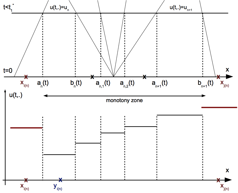
Figure 1: a zoom around a wave fan. The $\times$ symbols correspond to a subdivision in the neighborhood of a wave fan: we have here $P=\{y_{i(n)}\}$.

Second step - Let $(u_{0}^{n})_{n\geq 0}$ be a sequence of step functions in $BV^{s}$ such that $u_{0}^{n}\to u_{0}$ in $L^{1}_{loc}$ and a.e., with $TV^{s}u_{0}^{n}\leq TV^{s}u_{0}$ : this is ensured by Proposition 2.8.
Let $(f^{n})_{n\geq 0}$ be a sequence of piecewise affine functions such that $f^{n}\to f$ uniformly on every compact set.
Let $u^{n}$ be the solution of Problem (10) associated to the initial condition $u_{0}^{n}$ and the flux $f^{n}$. For all $t\geq 0$, $(u^{n}(t,\cdot))_{n\geq 0}$ is bounded in $L^{\infty}\cap BV^{s}$ thus it converges, extracting a subsequence if necessary, in $L^{1}_{loc}$ and a.e.
Similarly to the case of BV data ([2]), we can establish that the sequence $(u^{n})_{n\geq 0}$ is bounded in $Lip^{s}([0,+\infty[_{t},\,L^{1/s}_{loc}(\mathbb{R}_{x},\mathbb{R}))$: this is enough to get the convergence a.e. in $[0,+\infty[_{t}\times\mathbb{R}$ of some subsequence (still noted $(u^{n})$) towards a function $u$, entropy solution of the initial problem. Lastly Proposition 2.9 ensures that for all $t\geq 0$ and $n\in\mathbb{N}$, $TV^{s}u(t,\cdot)\leq TV^{s}u^{n}(t,\cdot)\leq TV^{s}u_{0}$, thus Theorem 3.1 holds.        $\square$

4 Smoothing effect for nonlinear degenerate convex fluxes

First we define the degeneracy of a nonlinear flux. Then we obtain a smoothing effect in the spirit of P.-D. Lax [15] and O. Oleinik [24]. Finally, we study the asymptotic behavior of entropy solutions as [19]. There is two main tools: the Lax-Oleinik formula and the $BV^{s}$ spaces. We refer the reader to the book of P.-D. Lax [17] for these results in the case of uniformly convex flux and also to [11] for detailed proofs.

4.1 Degenerate nonlinear flux

Definition 4.1 (degeneracy of a nonlinear convex flux)

Let $f$ belong to $C^{1}(I,\mathbb{R})$ where $I$ is an interval of $\mathbb{R}$. We say that the degeneracy of $f$ on $I$ is at least $p$ if the continuous derivative $a(u)=f^{\prime}(u)$ satisfies:

$$0<\inf_{I\times I}\frac{|a(u)-a(v)|}{|u-v|^{p}}$$ (12)

We call the lowest real number $p$, if it exists, the degeneracy measurement of uniform convexity on $I$. If there is no $p$ such that (12) is satisfied, we set $p=+\infty$.
Let $f\in C^{2}(I)$. We say that a real number $y\in I$ is a degeneracy point of $f$ in $I$ if $f^{\prime\prime}(y)=0$ (i.e. $y$ is a critical point of $a$).

If $f\in C^{2}(I)$ we can see easily that $p\geq 1$.

Remark 4.1

Condition (12) implies the strict monotonicity of $a(.)$ and then the strict convexity or concavity of the flux, but it is more general than the uniform convex case studied by P.-D. Lax in [15]. Indeed, (12) allows $f^{\prime\prime}$ to vanish as one can see below with the power law flux function.

We give some examples to illuminate this notion.

Example 4.1

Uniformly convex function: $\inf f^{\prime\prime}>0$.
The degeneracy is $p=1$.

This is the basic example studied by P.-D. Lax [15] with $I=\mathbb{R}$.

Example 4.2

Linear flux. The degeneracy is $p=+\infty$.

Example 4.3

Power convex functions $f(u)=\displaystyle\frac{|u|^{1+\alpha}}{1+\alpha}$, $\alpha>0$.
Let $I=[0,1]$, then $y=0$ is a degeneracy point and the degeneracy of $f$ in $I$ is $p=\max(1,\alpha)$.

This example is the basic example to obtain all the finite degeneracy $p\geq 1$.

Proof: the computation of $p$ is straightforward. The case $\alpha<1$ is left to the reader. The case $\alpha=1$ corresponds to the Burgers flux, the simplest example of an uniformly strictly convex flux. Let us study the more interesting case $\alpha>1$. It is clear that $p\geq\alpha$, else the fraction of Inequality (12) vanishes for $v=0$ and $u\rightarrow 0$. It suffices to study the case $p=\alpha$. Let $R(u,v)=\displaystyle\frac{|u^{\alpha}-v^{\alpha}|}{|u-v|^{\alpha}}$ for $u\neq v$. It suffices to study the case $u<v$ by symmetry: with $v=u+h,\;h>0$, $R(u,u+h)=\displaystyle\frac{(u+h)^{\alpha}-u^{\alpha}}{h^{\alpha}}=\phi(y)=(y+1)^{\alpha}-y^{\alpha}$, where $y=\displaystyle\frac{u}{h}\in[0,+\infty[$. Then $\displaystyle\inf_{y\geq 0}\phi(y)=2^{1-\alpha}>0$ which is enough to conclude.        $\square$

Example 4.4

Smooth degenerate convex flux.
Let $K$ be a compact interval, $f\in C^{\infty}(K,\mathbb{R})$ and let $a=f^{\prime}$ be an increasing function. We define classically the valuation of $f^{\prime\prime}$ by:

$$val[a](u)=\min\left\{k\geq 1,\frac{d^{k}a}{du^{k}}(u)\neq 0\right\}\in\{1,2,\dots\}\cup\{+\infty\}$$

then the degeneracy of $f$ on $K$ is $p=\displaystyle\max_{K}val[a]$.

We say that the flux is nonlinear if $p$ is finite.

This general example has been studied recently for the multidimensional case in [1, 14]. These examples allow to compute the parameter of degeneracy of any smooth flux given in the paper of P.-L. Lions, B. Perthame and E. Tadmor [18].

Proof: In the one dimensional case, the computation is easier. We give a simple proof for a nonlinear flux, i.e. the valuation is finite for each point of $K$. Let $R(u,v)=\displaystyle\frac{|a(u)-a(v)|}{|u-v|^{p}}$ for $u\neq v$. Since $R$ is a continuous function on $u\neq v$, positive outside the diagonal $\{u=v\}$, it suffices to study $R$ on the diagonal. Let $k$ be $val[a](u)$, $\displaystyle R(u,u)=\left\{\begin{array}[]{ccc}0&if&k>p,\\ |a^{(k)}(u)|&if&k=p,\\ +\infty&if&k<p.\end{array}\right.$
So the lowest $p$ in the neighborhood of $u$ is $p=val[a](u)$. Notice that the valuation is upper semi-continuous. So the maximum of the valuation on the compact $K$ exists and it is the lowest $p$ satisfying Definition 4.1 .        $\square$

4.2 Smoothing effect

We generalize the Oleinik one sided Lipschitz condition [24] to define an entropy solution on the scalar conservation law (10) and we prove that the Lax-Oleinik formula yields such condition for degenerate convex flux.

Definition 4.2 (One sided Hölder condition)

Let $f$ be a degenerate convex flux. Let $p\geq 1$ be a degeneracy parameter of $f$ on an interval $I$, and $0<s=\dfrac{1}{p}\leq 1$. Let be $u$ a weak solution of (10). Assume that $u$ belongs to $I$. This solution is called an entropy solution if for some positive constant $c$, for all $t>0$ and for almost all $(x,y)$ such that $x<y$ we have

$$u(t,y)-u(t,x) \leq c\,\frac{(y-x)^{s}}{t^{s}}.$$ (13)

If $-f$ is convex then we replace in Inequality (13) $u$ by $-u$.
As usual, the one sided condition implies the Lax entropy condition [6].

Theorem 4.1 ($BV^{s}$ smoothing effect for degenerate convex flux)

Let $K$ be the compact interval $[-M,M]$. Let $u_{0}$ belong to $L^{\infty}(\mathbb{R})$, $f\in C^{1}(\mathbb{R},\mathbb{R})$ and let $u$ be the unique entropy solution on $]0,+\infty[_{t}\times\mathbb{R}_{x}$ of the scalar conservation law (10) satisfying the one sided condition (13). Let $p$ be a degeneracy parameter of $f$ on $K$ and $0<s=\displaystyle\frac{1}{p}\leq 1$.
If $p$ is finite and $|u_{0}|\leq M$ then $u\in\mbox{\rm Lip}^{s}(]0,+\infty[_{t},L_{loc}^{1/s}(\mathbb{R}_{x},\mathbb{R}))$ and

$$\forall t>0,\,u(t,.)\in BV^{s}_{loc}(\mathbb{R}).$$

If $u_{0}$ is compactly supported then $u\in\mbox{\rm Lip}^{s}(]0,+\infty[_{t},L^{1/s}(\mathbb{R}_{x},\mathbb{R}))$ and there exists a constant $C$ such that

$$TV^{s}u(t,.)\leq C\left(1+\displaystyle\frac{1}{t}\right).$$

Remark 4.2

This entropy solution is the unique Kruzhkov entropy solution. It is well known for an uniformly convex flux [6], for the degenerate convex case see ([4].

Remark 4.3

This theorem gives the regularity conjectured by P.-L. Lions, B. Perthame and E. Tadmor in [18] for a non linear convex flux. This conjecture was stated in Sobolev spaces. The $W^{s,1}$ regularity with only $L^{\infty}$ initial data was first proved in [13]. We get the best $W^{s,p}$ regularity. Indeed by Proposition 2.10, this $BV^{s}$ regularity gives a $W^{s^{\prime},1/s}$ smoothing effect for all $s^{\prime}<s$.

Remark 4.4

We cannot expect a better regularity. Indeed, C. De Lellis and M. Westdickenberg give in [9] a piecewise smooth entropy solution which does not belong to $W^{s,1/s}$. Recently, in [4, 5], another examples, with continuous functions, are built. Indeed for each $\tau>s$ , there exists a smooth solution which belongs to $BV^{s}$ but not to $BV^{\tau}$.

Remark 4.5

For solutions with bounded entropy production and uniform convex flux, the optimal smoothing effect is reached in [12]. This class of solutions is larger than the class of entropy solutions. The optimal exponent is only $s=1/3$ ([9, 12]) instead of $s=1$ for uniformly convex fluxes.

Proof: we first recall the Lax-Oleinik formula for a general convex flux without assuming the uniform convexity. We assume only (12). With such an assumption the Lax-Oleinik formula is still valid ([4]). We know, thanks to Remark 4.1, that the function $a$ (or $-a$), is increasing. We assume here that the function $a$ is increasing on $K$. We can easily extend $a$ continuously on $\mathbb{R}$ with the same degeneracy parameter $p$ (using a suitable translated power function) then the function $a$ admits the inverse function $b$ on $\mathbb{R}$. The entropy solution is then given for all $t$ and almost all $x$ by the Lax-Oleinik formula:

$$u(t,x)=b\left(\frac{x-y}{t}\right)$$ (14)

where $y=y(t,x)$ minimizes, for $t$ and $x$ fixed, the function

$$G(t,x,y)=U_{0}(y)+t\,h\left(\frac{x-y}{t}\right)$$

with $\displaystyle U_{0}(y)=\int_{0}^{y}u_{0}(x)\,dx$, $a(0)=c$, $\displaystyle h(u)=\int_{c}^{u}b(v)\,dv$.

Geometrically, $y(t,x)$ has a simple interpretation. The function $u(.,.)$ is constant on the characteristic $x=y+ta(u_{0}(y))$: $u(t,x)=u_{0}(y)$ (before the formation of a shock). Indeed $a(u_{0}(y))=\displaystyle\frac{x-y}{t}$, so $b(a(u_{0}(y)))=b\left(\displaystyle\frac{x-y}{t}\right)=u_{0}(y)=u(t,x)$. The key point of the formula (14) is that $y(t,x)$ minimizes an explicit function, namely $y\mapsto G(t,x,y)$. Consequently $y(t,x)$ is not so far from $x$, more precisely:

$$|x-y(t,x)|\leq t\,\sup_{K}|a|.$$ (15)

Moreover, if $x_{1}<x_{2}$ then $y(t,x_{1})\leq y(t,x_{2})$, ([17, 11, 4]).

Condition (12) implies that $b$ belongs to $C^{s}(\mathbb{R},\mathbb{R})$ with $s=1/p$. Indeed we have for all $U,V\in a(K)$, with $u=b(U)$ and $v=b(V)$:

$$\frac{|b(U)-b(V)|}{|U-V|^{s}}=\frac{|u-v|}{|a(u)-a(v)|^{s}}=\left(\frac{|u-v|^{p}}{|a(u)-a(v)|}\right)^{s}\leq D^{s}=\frac{1}{C^{s}}$$

where $\displaystyle 0<C=\inf_{K\times K}\frac{|a(u)-a(v)|}{|u-v|^{p}}$.

We are now able to prove the $BV^{s}$ smoothing effect. Fix $T>0$ and $I=[a,b]$: we want to bound $TV^{s}u\{I\}$. Let $x_{1},\,x_{2}\in I$ and $y_{i}=y(t,x_{i})$, then

$$|u(T,x_{1})-u(T,x_{2})|^{p} = \displaystyle\left|b\left(\frac{x_{1}-y_{1}}{T}\right)-b\left(\frac{x_{2}-y_{2}}{T}\right)\right|^{p}$$

$$\leq \left(D^{s}\left|\frac{x_{1}-y_{1}}{T}-\frac{x_{2}-y_{2}}{T}\right|^{s}\right)^{p}.$$

The condition $sp=1$ yields

$$|u(T,x_{1})-u(T,x_{2})|^{p}\leq\displaystyle D\left|\frac{x_{1}-x_{2}}{T}\right|+D\left|\frac{y_{1}-y_{2}}{T}\right|.$$

We now compute $TV^{s}u\{\sigma\}$ for a subdivision $\sigma=\{x_{0}<x_{1}<\cdots<x_{n}\}$ of $I$. Then

$$TV^{s}u\{\sigma\}\leq\frac{D}{T}(x_{n}-x_{0}+y_{n}-y_{0})\leq\frac{D}{T}(2(b-a)+T\sup_{K}|a|).$$ (16)

Then $TV^{s}u\{I\}$ keeps the same bound.
We can precise the previous bounds. First, we obtain the one sided Hölder condition (13), which implies that the solution is an entropy solution. We know that if $x_{1}<x_{2}$ then

$$y_{1}=y(t,x_{1})\leq y(t,x_{2})=y_{2}.$$

Moreover

$$u(t,x_{2})-u(t,x_{1})=b\left(\frac{x_{2}-y_{2}}{t}\right)-b\left(\frac{x_{1}-y_{1}}{t}\right)\leq b\left(\frac{x_{2}-y_{2}}{t}\right)-b\left(\frac{x_{1}-y_{1}}{t}\right)$$

because $b$ is increasing. But, $b(\frac{x_{2}-y_{2}}{t})-b(\frac{x_{1}-y_{1}}{t})\geq 0$ because $x_{2}\geq x_{1}$. Then

$$u(t,x_{2})-u(t,x_{1})\leq\left|b\left(\frac{x_{2}-y_{2}}{t}\right)-b\left(\frac{x_{1}-y_{1}}{t}\right)\right|\leq D^{s}\left|\frac{x_{2}-x_{1}}{t}\right|^{s}=D^{s}\frac{(x_{2}-x_{1})^{s}}{t^{s}}.$$

We can improve the $TV^{s}$ bound for a compactly supported initial data. For any $t$, the solution stays compactly supported (but the size of this support depends on $t$). Fix $T=1$. Inequality (16) gives $u\in BV^{s}(\mathbb{R})$.
For $t\geq T$, Theorem 3.1 implies $TV^{s}u(t,.)\leq TV^{s}u(T,.)=C_{1}$ and for $0<t\leq T$, Inequality (16) implies $TV^{s}u(t,.)\leq C_{0}(1+\displaystyle\frac{1}{t})$, then $\forall t>0$, $TV^{s}u(t,.)\leq C(1+\displaystyle\frac{1}{t})$.
Theorem 3.1 shows that $u\in\mbox{\rm Lip}^{s}(]0,+\infty[_{t},L^{1/s}(\mathbb{R}_{x},\mathbb{R}))$.
Fo the general case, the estimate is only locally valid with respect to the space variable.        $\square$

Proposition 4.1

The unique entropy solution of Theorem 4.1 satisfies the folowing decay $\displaystyle TV^{s}_{+}u(T,.)\{[a,b]\}\leq D\frac{|b-a|}{T}$ for some positive constant $D$.

Proof: it is a direct consequence of the one sided condition (13).        $\square$

4.3 Asymptotic behavior of entropy solutions

The smoothing effect is sometimes related to the asymptotic behavior for large time ([15, 16, 17]). We investigate briefly classical decays under assumption (12). Indeed the decay of the solution with compact support depends on one more parameter.

Theorem 4.2 (Decay for large time)

Let be $u_{0}\in L^{1}\cap L^{\infty}(\mathbb{R})$, $|u_{0}|\leq M$, $K=[-M,M]$. Assume that $f\in C^{1}(\mathbb{R},\mathbb{R})$ satisfies Condition (12) with $a=f^{\prime}$, $p$ the degeneracy of $f$ on $K$, $s=1/p$. Let $u$ be the unique entropy solution on $]0,+\infty[_{t}\times\mathbb{R}_{x}$ of (10) and $b$ the inverse function of the function $a$ on $a(K)$.
If there exists $q>0$ such that

$$0<\inf_{U\in a(K)}\frac{|b(U-a(0))|}{|U|^{q}}$$ (17)

then there exists $C>0$ such that

$$|u(t,x)|\leq\frac{C}{t^{d}},\qquad d=\frac{s}{1+q}.$$

Originally, P.-D. Lax found this optimal decay in the 50’ for strictly convex flux with $d=\displaystyle\frac{1}{2}$ since $s=q=1$ [15].
For power function $f(u)=|u|^{1+\alpha}$, $\alpha>1$, we have $d=\displaystyle\frac{s}{1+s}<\displaystyle\frac{1}{2}$ since $s=\displaystyle q=1/\alpha$. For the simplest degenerate convex case: the cubic convex flux, we only have $d=\displaystyle\frac{1}{3}$. This decay is slower than classical Lax decay which is $\displaystyle\frac{1}{\sqrt{t}}$.
Remark that $q\geq s$. Assume that without loss of generality $a(0)=0$ and $J=a(K)=[0,1]$. Then $|b(x)-b(y)|\leq C|x-y|^{s}$ since $b$ is in $C^{s}(J)$. Moreover, there exists $D>0$ such that $D|x|^{q}\leq|b(x)|$ by (17), so $Dx^{q}\leq Cx^{s}$ on $[0,1]$ then we have $q\geq s$.
We give some examples with $q>s$. On $K=J=[0,1]$, with $f(u)=\displaystyle\frac{u^{1+\alpha}}{1+\alpha},\,0<\alpha<1$ we have $s=1,\,q=\displaystyle\frac{1}{\alpha}>1=s$.

Proof: the proof is a slight modification of the original Lax’s proof, [17]. We use the Lax-Oleinik formula with the notations of the proof of Theorem 4.1, so we have to extend the function $a$ on $\mathbb{R}$. We have

$$\forall y\in\mathbb{R},\,-d_{2} \leq U_{0}(y)=\int_{0}^{y}u_{0}(x)\,dx$$

$$\leq d_{2}=\max\left(\int_{0}^{+\infty}|u_{0}(x)|dx,\int^{0}_{-\infty}|u_{0}(x)|dx\right).$$

Notice that $\min G\leq d_{2}$. Since $h$ is a convex nonnegative function which vanishes only at $c=a(0)$, it suffices to take $y=x-c\,t$ so $G(t,x,y)=U_{0}(y)$. Integrating Inequality (17), there exists a constant $d_{1}>0$ such that for $z\in J=a(K)$,

$$h(z)\geq d_{1}|z-c|^{1+q}.$$

Let $y=y(t,x)$ be the minimizer of $G(t,x,.)$.
Notice that $\displaystyle\frac{x-y}{t}\in J$ since $x-y=t\,a(u_{0}(y))$. Now, we have the inequality

$$d_{2}\geq G(t,x,y)\geq-d_{2}+td_{1}\left|\frac{x-y}{t}-c\right|^{1+q}$$

then

$$2\,d_{2}\geq t\,d_{1}\left|\frac{x-y}{t}-c\right|^{1+q}$$

and then

$$\displaystyle\left(\frac{2d_{2}}{d_{1}t}\right)^{1/(1+q)} \geq \left|\frac{x-y}{t}-c\right|.$$ (18)

Since $b\in C^{s}$, we have $|b(z)|=|b(z)-b(c)|\leq D^{s}|z-c|^{s}$ .
The Lax-Oleinik formula (14) and Inequality (18) conclude the proof:

$$\displaystyle|u(t,x)|=\left|b\left(\frac{x-y}{t}\right)\right| \leq \displaystyle D^{s}\left(\frac{2\,d_{2}}{d_{1}t}\right)^{s/(1+q)}.$$

$\square$

The periodic case is much simpler and only depends on the degeneracy of $f$.

Theorem 4.3 (Decay for periodic solutions)

Let $u_{0}$ be a P-periodic bounded function, $m=\displaystyle\frac{1}{P}\int_{0}^{P}u_{0}(x)dx$, $|u_{0}|\leq M$,
$K=[-M,M]$, let $u$ be the unique entropy solution on $]0,+\infty[_{t}\times\mathbb{R}_{x}$ of (10), $f\in C^{1}(\mathbb{R},\mathbb{R})$. If the degeneracy $p$ of $f$ on $K$ is finite then there exists a constant $C$ such that

$$|u(t,x)-m|\leq\frac{C}{t^{s}},\,s=\frac{1}{p}.$$

For uniform convex flux we have the classical case with $s=1$, [15].
For power function $f(u)=|u|^{1+\alpha}$ with $\alpha>1$ we have $s=\displaystyle 1/\alpha$. For instance, for the cubic convex flux, $s=\displaystyle\frac{1}{2}$.

Proof: first notice that $u(t,.)$ is periodic with the same period $P$ and the same mean value $m$. We have thanks to the one side condition (13) the inequality

$$u(t,y)-u(t,x)\leq C\frac{(y-x)^{s}}{t^{s}}\leq C\frac{P^{s}}{t^{s}}$$

for $0\leq y-x\leq P$. Assume that $m=0$ without loss of generality. Fix $x$. If $u(t,x)<0$, there exists $y$ in $[x,x+P]$ such that $u(t,y)>0$ since $m=0$. Then

$$|u(t,x)|\leq|u(t,x)|+|u(t,y)|\leq|u(t,y)-u(t,x)|=u(t,y)-u(t,x)\leq C\frac{P^{s}}{t^{s}}.$$

The same argument holds if $u(t,x)>0$, which concludes the proof.        $\square$

References

- [1] F. Berthelin, S. Junca. Averaging lemmas with a force term in the transport equation. J. Math. Pures Appl., (), , No , , .
- [2] A. Bressan. Hyperbolic Systems of Conservation Laws, The One-Dimensional Cauchy Problem. Oxford lecture series in mathematics and its applications. Oxford University Press, , .
- [3] H. Brezis, L. Nirenberg. Degree theory and BMO; Part I: Compact Manifolds without boundaries. Selecta Mathematica, New series, Vol . , No., .
- [4] P. Castelli. Lois de conservation scalaires, exemples de solutions et effet régularisant (in French). Master Thesis. Université de Nice Sophia Antipolis .
- [5] P. Castelli, S. Junca. Oscillating waves and the maximal smoothing effect for one dimensional nonlinear conservation laws. (oai:hal.archives-ouvertes.fr:hal-00785529), .
- [6] C.-M Dafermos. Hyperbolic Conservation Laws in Continuum Physics. Springer Verlag, Berlin-Heidelberg, .
- [7] C. De Lellis, F. Otto, M. Westdickenberg. Structure of entropy solutions for multidimensional scalar conservation laws. Arch. ration. Mech. Anal. 170, No. , , .
- [8] C. De Lellis, T. Rivière. The rectifiability of entropy measures in one space dimension. J. Math. Pures Appl. (9) 82, no. 10, 1343–1367, .
- [9] C. De Lellis, M. Westdickenberg. On the optimality of velocity averaging lemmas. Ann. I. H. Poincaré AN, , No. , , .
- [10] R.-A. DeVore. Nonlinear Approximation. Acta Numerica, , .
- [11] L.-C. Evans. Partial Differential Equations. Graduate Studies in Mathematics, A.M.S., , .
- [12] F. Golse, B. Perthame. Optimal regularizing effect for scalar conservation laws. (arXiv:1112.2309v2), (2012).
- [13] P.-E. Jabin. Some regularizing methods for transport equations and the regularity of solutions to scalar conservation laws. Séminaire: Equations aux Dérivées Partielles, Ecole Polytech. Palaiseau. 20082009, Exp. No. XVI, .
- [14] S. Junca. High frequency waves and the maximal smoothing effect for nonlinear scalar conservation laws. oai:hal.archives-ouvertes.fr:hal-00576662, .
- [15] P.-D. Lax. Hyperbolic systems of conservation laws, II. Comm. Pure Appl. Math., , , .
- [16] P.-D. Lax. The formation and decay of shock waves. Amer. Math. Monthly, .
- [17] P.-D. Lax. Hyperbolic partial differential equations. Courant Lecture Notes in Mathematics, . American Mathematical Society, Providence, RI, .
- [18] P.-L. Lions, B. Perthame, E. Tadmor. A kinetic formulation of multidimensional scalar conservation laws and related equations. J. Amer. Math. Soc., , , .
- [19] T.-P. Liu, M. Pierre. Source-solutions and asymptotic behavior in conservation laws. Journal of hyperbolic Differential Equations, , , .
- [20] E.-R. Love, L.-C. Young. Sur une classe de fonctionnelles linéaires. Fund. Math., , , .
- [21] J. Musielak, W. Orlicz. On space of functions of finite generalized variation. Bull. Acad. Pol. Sc. , , .
- [22] J. Musielak, W. Orlicz. On generalized variations. Studia mathematica XVIII, , .
- [23] J. Musielak. Orlicz spaces and modular spaces Lecture Notes in mathematics, Springer Verlag, Berlin, , .
- [24] O.-A. Oleinik. Discontinuous solutions of nonlinear differential equations, (in russian 1957), Transl. Amer. Math. Soc., Ser. , , , .
- [25] E. Tadmor, T. Tao. Velocity averaging, kinetic formulations, and regularizing effectsin quasi-linear PDEs. Comm. Pure Appl. Math. , No. , , .
- [26] L. Tartar. An introduction to Sobolev Spaces and Interpolation Spaces. Lecture Notes of the Unione Matematica Italiana, Springer, .
- [27] N. Wiener. The quadratic variation of a function and its Fourier coefficients. Journ. Mass. Inst. of Technology , , .