Thirring model at finite density in $0+1$ dimensions
with stochastic quantization: Crosscheck with an exact solution

Abstract

We consider a generalized Thirring model in $0+1$ dimensions at finite density. In order to deal with the resulting sign problem we employ stochastic quantization, i.e., a complex Langevin evolution. We investigate the convergence properties of this approach and check in which parameter regions complex Langevin evolutions are applicable in this setting. To this end we derive numerous analytical results and compare directly with numerical results. In addition we employ indirect indicators to check for correctness. Finally we interpret and discuss our findings.

I Introduction

Despite all efforts, one of the outstanding problems of lattice field theory until this day is the sign problem. The introduction of a finite chemical potential $\mu>0$ renders the path integral measure complex and rapidly oscillating in many theories of interest, like quantum chromodynamics (QCD) in $3+1$ dimensions. The oscillatory behavior significantly increases the numerical costs, in particular in the continuum limit. A hard sign problem exists for theories where the costs grow more than polynomially with the volume. This obstacle hinders numerical ab initio studies of strongly interacting matter under extreme conditions and the understanding of the phase diagram of QCD. There is no satisfactory solution known to the sign problem, despite the large number of proposed solutions.

Among the proposed solutions we can find reweighting techniques, Taylor expansions about $\mu=0$, extrapolations from imaginary chemical potential, the introduction of dual variables and a canonical ensemble approach. For recent reviews see e.g. de Forcrand (2009); Lombardo (2007). However, due to the overlap problem reweighting techniques are computationally expensive and can only be used for small $\mu$, while the numerical determination of Taylor coefficients is noisy and the expansion converges slowly Karsch et al. (2011). Also the continuation from imaginary chemical potential is a nontrivial task Lombardo (2006). The application of dual variables and the canonical ensemble approach is still under active research, see e.g. Schmidt et al. (2012); Mercado et al. (2013) for dual observables and Alexandru et al. (2005); Alexandru and Wenger (2011) for simulations with canonical ensembles.

In this paper we employ a different approach. Parisi proposed already in 1983 that stochastic quantization Parisi and Wu (1981)—for a review see e.g. Damgaard and Huffel (1987)—could circumvent the sign problem in terms of a complex Langevin evolution Parisi (1983). However, it is well known that the Langevin evolution may converge towards unphysical fixed points. It has been successfully applied to the SU(3) spin model Karsch and Wyld (1985); Aarts and James (2012), to an effective theory of QCD in the strong-coupling limit Bilic et al. (1988), simple models of quantum chromodynamics Aarts and Stamatescu (2008); Aarts and Splittorff (2010) and to the relativistic Bose gas Aarts (2009a, b) at finite density. Furthermore it has been applied to quantum fields in Minkowski time Berges et al. (2007); Berges and Sexty (2008), also in nonequilibrium Berges and Stamatescu (2005). Counterexamples are given by the three-dimensional XY model at finite chemical potential for small $\beta$ Aarts and James (2010a) and in cases of gauge theories with static charges Ambjorn et al. (1986). Early investigations of complex Langevin evolutions can be found in Hamber and Ren (1985); Flower et al. (1986); Ilgenfritz (1986), while for reviews see e.g. Aarts (2012, 2009c). Recently, a set of consistency conditions indicating correct convergence could be derived Aarts et al. (2010a, 2011a, 2011b). When truncating this infinite tower of identities one obtains necessary conditions for correctness.

In this work we apply a complex Langevin evolution to a generalized Thirring model at finite density. Here it serves us as a model theory to check for the applicability of this method. Our results extend the studies carried out in Spielmann (2010), which led to ambiguous results. In this paper we restrict ourselves to the case of $0+1$ dimensions and deal with the question of whether a complex Langevin evolution can enable finite density calculations in this setting. Further investigations of this approach in the $2+1$-dimensional generalized Thirring model are presented in Pawlowski and Zielinski (2013). The $2+1$-dimensional model appears for example in effective theories of high temperature superconductors and graphene, see e.g. Gies and Janssen (2010) and references given therein. It is also worth mentioning that in the case of the three-dimensional massless Thirring model, a fermion bag approach was successfully applied in Chandrasekharan and Li (2012).

We organized the paper as follows: In Sec. II we introduce a generalized Thirring model and its formulation on the lattice. We discuss the Langevin equation and its numerical implementation. In Sec. III we present a closed expression for the partition function of the lattice theory and derive some observables of interest. We also discuss additional indicators to evaluate the convergence properties of the complex Langevin evolution. In Sec. IV we discuss the results of the numerical part of this work and aim to answer the question in which parameter regime results are reliable. We end this paper with concluding remarks in Sec. V.

II The Generalized Thirring Model

II.1 Continuum formulation

We consider a generalization of the Thirring model. The historical model was introduced in 1958 by Walter E. Thirring and is one of the rare examples of an exactly solvable quantum field theory Thirring (1958). While the original model describes self-interaction fermions in $1+1$ dimensions, we consider $N_{f}$ fermion flavors at finite density.

We begin with a generalization to $d$ dimensions and then later specialize to the case of $0+1$ dimensions. The Euclidean Lagrangian in the continuum reads

$$\mathscr{L}_{\Psi}=\sum_{i=1}^{N_{f}}\overline{\Psi}_{i}\left(\not{\partial}+m_{i}+\mu_{i}\gamma_{0}\right)\Psi_{i}\\ +\frac{g^{2}}{2N_{f}}\left(\sum_{i=1}^{N_{f}}\overline{\Psi}_{i}\gamma_{\nu}\Psi_{i}\right)^{2}.$$ (1)

The index $i=1,\ldots,N_{f}$ enumerates fermion flavors, $m_{i}$ and $\mu_{i}$ denote the bare mass and bare fermion chemical potential of the respective flavor and $g^{2}$ is the bare coupling strength. The $\gamma$ matrices satisfy the Clifford algebra $\left\{\gamma_{\mu},\gamma_{\nu}\right\}=2\delta_{\mu\nu}\mathbbm{1}$.

The model shows breaking of chiral symmetry at $\mu=0$ in $2+1$ dimensions Christofi et al. (2007). For the $1+1$-dimensional Thirring model, the equivalence to the sine-Gordon model can be shown Coleman (1975); Benfatto et al. (2009).

The four-point interaction can be resolved with the introduction of an auxiliary field $A_{\nu}$. This formulation reads

$$\mathscr{L}=\sum_{i}\overline{\Psi}_{i}\left(\not{\partial}+\textrm{i}\not{A}+m_{i}+\mu_{i}\gamma_{0}\right)\Psi_{i}+N_{f}\beta A_{\nu}^{2}.$$ (2)

Here we introduced the inverse coupling $\beta=1/\left(2g^{2}\right)$. When integrating $A_{\nu}$ out, we recover (1). Although the auxiliary field $A_{\nu}$ is not a gauge field, the model can be interpreted as a more general gauge theory after gauge fixing, see e.g. Itoh et al. (1995). After integrating out the fermionic degrees of freedom we find

$$Z =\intop\mathscr{D}A\,\left(\prod_{i}\det K_{i}\right)\,e^{-S_{A}}=\intop\mathscr{D}A\,e^{-S_{\textrm{eff}}},$$

$$S_{A} =N_{f}\beta\intop_{0}^{1/T}\textrm{d}t\intop\textrm{d}^{d-1}\mathbf{x}\,A_{\nu}^{2}.$$ (3)

Here we introduced the temperature $T$ and $K_{i}=\not{\partial}+\textrm{i}\not{A}+m_{i}+\mu_{i}\gamma_{0}$. Including the fermion determinant in the exponential term yields

$$S_{\textrm{eff}}=S_{A}-\sum_{i}\operatorname{Tr}\log K_{i}.$$ (4)

For the fermion determinant the relation

$$\det K_{i}\left(\mu\right)=\left[\det K_{i}\left(-\mu^{\star}\right)\right]^{\star}$$ (5)

holds, thus rendering the path integral measure complex for $\mu>0$. At vanishing or purely imaginary chemical potential, the determinant is real and the theory is free of a sign problem. If the fermion determinant is replaced by its modulus, we refer to this as the phase-quenched case. Physically this corresponds to the introduction of an isospin chemical potential.

Like quantum chromodynamics, the Thirring model exhibits Silver Blaze behavior Cohen (2003); Splittorff and Verbaarschot (2007). It implies that at vanishing temperature there is a threshold $\mu_{c}$, so that observables are independent of the chemical potential $\mu$ for $\mu<\mu_{c}$. While in the full theory the onset is given by the physical fermion mass $m_{\textrm{phys}}$, in the phase-quenched theory we have $\mu_{c}=m_{\pi}/2$, where $m_{\pi}$ is the physical pion mass.

II.2 Lattice formulation

We consider the case of $0+1$ dimensions—corresponding to a quantum mechanical system—with lattice spacing $a$ and $N_{t}$ lattice points. We employ staggered fermions Kogut and Susskind (1975); Banks et al. (1976, 1977); Susskind (1977) and denote the number of lattice flavors, i.e., the number of staggered fermion fields, by $\mathcal{N}$. Furthermore we assume that $N_{t}$ is even, as otherwise the formulation of staggered fermions is conceptually problematic and (5) is violated. In order to introduce a finite chemical potential $\mu$, we use the prescription by Hasenfratz and Karsch Hasenfratz and Karsch (1983). For notational ease we refer to the one-component auxiliary field as $A_{t}=A_{0}(x=t)$ and all dimensionful quantities are scaled dimensionless by appropriate powers of $a$. Furthermore we introduce the hopping parameter $\kappa=1/\left(2m\right)$. The temperature corresponds to the inverse temporal extension $T=N_{t}^{-1}$.

Using this formulation the lattice partition function reads

$$Z=\intop_{-\infty}^{\infty}\prod_{t=1}^{N_{t}}\textrm{d}A_{t}\,\left(\prod_{i}\det K_{i}\right)\,e^{-S_{A}}$$ (6)

with $S_{A}=\frac{1}{2}\mathcal{N}\beta\sum_{t}A_{t}^{2}$ and flavor index $i=1,\ldots,\mathcal{N}$. The fermion matrix takes the form

$$K_{i}\left(t,\tau\right)=\frac{1}{2}\left(1+\textrm{i}A_{t}\right)e^{\mu_{i}}\delta_{t+1,\tau}\\ -\frac{1}{2}\left(1-\textrm{i}A_{\tau}\right)e^{-\mu_{i}}\delta_{t-1,\tau}+m_{i}\delta_{t\tau},$$ (7)

where we impose antiperiodic boundary conditions, cf. Del Debbio and Hands (1996); Spielmann (2010). In our analysis we focus on a few observables, namely the fermion density and condensate, the energy density and the phase factor of the fermion determinant. In the following, sums over the flavor index $i$ are not implied. The fermion density of a given flavor is given by

$$\left\langle n_{i}\right\rangle=\frac{1}{N_{t}}\left(\frac{\partial\log Z}{\partial\mu_{i}}\right)_{T}=\frac{1}{N_{t}}\left\langle\operatorname{Tr}\left(\frac{\partial K_{i}}{\partial\mu_{i}}K_{i}^{-1}\right)\right\rangle.$$ (8)

The fermion condensate follows from

$$\left\langle\overline{\chi}_{i}\chi_{i}\right\rangle=\frac{1}{N_{t}}\left(\frac{\partial\log Z}{\partial m_{i}}\right)_{T,\mu_{i}}=\frac{1}{N_{t}}\left\langle\operatorname{Tr}K_{i}^{-1}\right\rangle$$ (9)

and the energy density reads

$$\left\langle\varepsilon_{i}\right\rangle=-\left(\frac{\partial\log Z}{\partial N_{t}}\right)_{\mu_{i}}+\mu_{i}\left\langle n_{i}\right\rangle,$$ (10)

which we normalize to $\left\langle\varepsilon_{i}\right\rangle\left(\mu=0\right)=0$.

The phase factor of the determinant is defined by $\exp\left(\textrm{i}\phi\right)=\det K/\left|\det K\right|$. It can be expressed in terms of the partition function

$$Z_{\mathcal{N}}=\intop_{-\infty}^{\infty}\prod_{t}\textrm{d}A_{t}\,\left(\det K\right)^{\mathcal{N}}\,e^{-S_{A}},$$ (11)

for $\mathcal{N}$ degenerated flavors and $Z_{\mathcal{N}}^{\textrm{pq}}$ for the phase-quenched case, where the fermion determinant in (11) is replaced by its modulus. The expectation value of $\exp\left(\textrm{i}\mathcal{N}\phi\right)$ follows in the $\mathcal{N}$ flavor phase-quenched theory Han and Stephanov (2008); Andersen et al. (2010) as

$$\left\langle e^{\textrm{i}\mathcal{N}\phi}\right\rangle_{\mathcal{N}}^{\textrm{pq}}=\frac{Z_{\mathcal{N}}}{Z_{\mathcal{N}}^{\textrm{pq}}}\in\left[0,1\right].$$ (12)

A value close to zero indicates a rapidly oscillating path integral measure with a severe sign problem.

II.3 Complex Langevin evolution

The idea of stochastic quantization is that observables in a Euclidean quantum field theory can be obtained as the equilibrium values of a statistical system coupled to a heat bath Damgaard and Huffel (1987). The problem of quantizing a field theory is then reduced to finding the static solutions of an associated Langevin equation. If the action is real and bounded from below, correctness of this approach can be ensured. We can also formally generalize to the case of a complex action Parisi (1983). This situation naturally arises when considering field theories at finite density. Until this day there is a lack of rigor mathematical understanding regarding the validity of this procedure. However, in cases where it is converging correctly one has a very elegant solution for the sign problem at hand.

We aim to check for the applicability of complex Langevin evolutions to the Thirring model. To this end we have to find the static solution of the Langevin equation

$$\frac{\partial}{\partial\Theta}A_{t}\left(\Theta\right)=-\frac{\delta S_{\textrm{eff}}\left[A\right]}{\delta A_{t}\left(\Theta\right)}+\sqrt{2}\,\eta_{t}\left(\Theta\right),$$ (13)

where $\Theta$ denotes a fictitious time. The noise term $\eta_{t}\left(\Theta\right)$ follows a Gaussian distribution with

$$\left\langle\eta_{t}\left(\Theta\right)\right\rangle =0,$$

$$\left\langle\eta_{t}\left(\Theta\right)\eta_{t^{\prime}}\left(\Theta^{\prime}\right)\right\rangle =\delta\left(t-t^{\prime}\right)\delta\left(\Theta-\Theta^{\prime}\right).$$ (14)

A simple approach to solve the Langevin equation numerically is a first order integration scheme with fixed stepsize $\epsilon_{L}$. Higher order integration schemes of $\mathcal{O}(\epsilon_{L}^{3/2})$ have been employed in the literature too Chang (1987); Aarts and James (2012). However, in some models fixed stepsize integration schemes fail due to the occurrence of run-away trajectories, which can be avoided by the use of an adaptive stepsize Ambjorn and Yang (1985); Aarts et al. (2010b). Although a constant stepsize proved here to be sufficient Spielmann (2010), we employ an adaptive stepsize algorithm due to better convergence properties. For $\mathcal{N}$ degenerated flavors our discretization of (13) reads

$$A_{t}\left(\Theta+\epsilon_{L}\right)=A_{t}\left(\Theta\right)+\epsilon_{L}D_{t}\left(\Theta\right)+\sqrt{2\epsilon_{L}}\,\eta_{t}\left(\Theta\right)$$ (15)

with drift term

$$D_{t}\left(\Theta\right)=-\mathcal{N}\beta A_{t}\left(\Theta\right)\\ +\frac{\mathcal{N}\textrm{i}}{2}\left[K^{-1}\left(t+1,t\right)e^{\mu}+K^{-1}\left(t,t+1\right)e^{-\mu}\right].$$ (16)

After each integration step the stepsize $\epsilon_{L}$ will be updated according to

$$\epsilon_{L}\equiv\epsilon_{L}\left(\Theta\right)=\frac{\delta}{\max_{t}\left|D_{t}\left(\Theta\right)\right|}$$ (17)

with stepsize parameter $\delta=10^{-3}$ (compare to Spielmann (2010)).

It is possible to generalize the real noise term in (15) to an imaginary one Spielmann (2010) via the replacement

$$\eta_{t}\left(\Theta\right)\;\to\;\sqrt{\mathcal{I}+1}\operatorname{Re}\eta_{t}\left(\Theta\right)+\textrm{i}\sqrt{\mathcal{I}}\operatorname{Im}\eta_{t}\left(\Theta\right)$$ (18)

with $\mathcal{I}\geq 0$. The noise correlators then read

$$\left\langle\operatorname{Re}\eta_{t}\left(\Theta\right)\operatorname{Re}\eta_{t^{\prime}}\left(\Theta^{\prime}\right)\right\rangle =\left\langle\operatorname{Im}\eta_{t}\left(\Theta\right)\operatorname{Im}\eta_{t^{\prime}}\left(\Theta^{\prime}\right)\right\rangle$$

$$=\delta\left(t-t^{\prime}\right)\delta\left(\Theta-\Theta^{\prime}\right)$$ (19)

and $\left\langle\operatorname{Re}\eta_{t}\left(\Theta\right)\operatorname{Im}\eta_{t^{\prime}}\left(\Theta^{\prime}\right)\right\rangle=0$. Assuming correctness of the complex Langevin evolution and numerical stability, we expect expectation values to be independent of $\mathcal{I}$.

III Analytical Results

III.1 Exact partition function

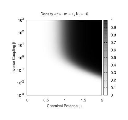
(a) Plot of the fermion density $\left\langle n\right\rangle$.

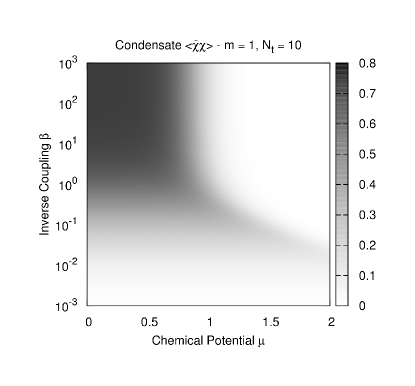
(b) Plot of the fermion condensate $\left\langle\overline{\chi}\chi\right\rangle$.

Figure 1: In the phase structure in $d=0+1$ we find a condensed phase for large $\mu$.

We begin with the partition function for one staggered fermion field, i.e., $\mathcal{N}=1$. We incorporate antiperiodic boundary conditions and for brevity we introduce

$$\mathfrak{B}_{\pm} =\frac{1}{2\left(2\kappa\right)^{N_{t}}}\left(1\pm\sqrt{\mathfrak{B}_{c}/\beta}\right)^{N_{t}},$$

$$\mathfrak{B}_{c} =\beta+4\left(\beta+1\right)\kappa^{2}.$$ (20)

Then the partition function (6) reads

$$Z_{1}=2\left(\frac{\pi}{2\beta}\right)^{N_{t}/2}\left[\mathfrak{B}_{+}+\mathfrak{B}_{-}+\cosh\left(N_{t}\mu\right)\right].$$ (21)

This can be shown for example by systematic saturation of the Grassmann integral or the help of the determinant identities in Molinari (2008). For the fermion density we find

$$\left\langle n\right\rangle=\frac{\sinh\left(\mu/T\right)}{\mathfrak{B}_{+}+\mathfrak{B}_{-}+\cosh\left(\mu/T\right)},$$ (22)

while the fermion condensate is given by

$$\left\langle\overline{\chi}\chi\right\rangle=\frac{2\kappa\sqrt{\beta/\mathfrak{B}_{c}}\left(\mathfrak{B}_{+}-\mathfrak{B}_{-}\right)}{\mathfrak{B}_{+}+\mathfrak{B}_{-}+\cosh\left(\mu/T\right)}.$$ (23)

The expression for the energy density is rather lengthy and we will not quote it here explicitly. Figure 1 shows the dependence of these observables on both $\beta$ and $\mu$. For large $\mu$ we find a condensed phase, which is well separated for large $N_{t}$.

As it turns out, we can take the continuum limit of the density $\left\langle n\right\rangle$ analytically. To this end we recover the physical units of all dimensionful quantities by reintroducing the lattice spacing $a$. We fix the dimensionful temperature $T^{-1}=aN_{t}$, express the lattice spacing $a$ as a function of the number of lattice points $N_{t}$ and take the limit $N_{t}\to\infty$. We obtain

$$\left\langle n\right\rangle_{\textrm{cont}}=\frac{\sinh\left(\frac{\mu}{T}\right)}{\frac{1}{2}\exp\left(\frac{\kappa-\beta}{2T\beta\kappa}\right)\left[1+\exp\left(\frac{1}{T\kappa}\right)\right]+\cosh\left(\frac{\mu}{T}\right)},$$ (24)

where all units are explicitly dimensionful. In the zero temperature limit $T\to 0$ we find $\left\langle n\right\rangle_{\textrm{cont}}=\Theta\left(\mu-m_{\textrm{phys}}\right)$ with physical fermion mass $m_{\textrm{phys}}=m+g^{2}$ and bare mass $m$.

III.2 Several flavors

We also considered the case of more than one lattice flavor, but only quote here the simplest case of (11) for $N_{t}=2$ lattice points and $\mathcal{N}=2$ staggered fermion fields

$$Z_{2}=\frac{\pi}{32\beta^{3}\kappa^{4}}\left[2\beta^{2}+4\beta\kappa^{2}+8\beta^{2}\kappa^{2}+5\kappa^{4}\right.\\ +12\beta\kappa^{4}+12\beta^{2}\kappa^{4}+8\beta^{2}\kappa^{2}\cosh\left(2\mu\right)\\ +\kappa^{4}\cosh\left(4\mu\right)+8\beta\kappa^{4}\cosh\left(2\mu\right)-4\beta\kappa^{4}\cosh\left(4\mu\right)\\ \left.+16\beta^{2}\kappa^{4}\cosh\left(2\mu\right)+4\beta^{2}\kappa^{4}\cosh\left(4\mu\right)\right].$$ (25)

We observe that for two flavors the density, condensate and energy density have plateaus in the range of $\beta\approx 0.3\text{--}1.2$, see also Fig. 9. They appear between the onset to the condensed phase and saturation of the density. The height of the plateau depends on the masses of the flavors, and in the case of degenerated flavors it is exactly at half of the maximum value of $\left\langle n\right\rangle$ or $\left\langle\overline{\chi}\chi\right\rangle$, respectively. If $\beta$ is very small or large, the plateaus eventually disappear. For large $\beta$ this can be understood from the weak coupling limit, see Sec. III.3. The existence of these plateaus on the lattice is further confirmed by a heavy dense limit Pawlowski and Zielinski (2013) and the Monte-Carlo studies in Sec. IV.4. In the general case of $\mathcal{N}$ flavors, we can find up to $\mathcal{N}-1$ intermediate plateaus in these observables. We give a natural explanation of these structures in the Appendix.

III.3 Weak coupling limit

In the limit of $\beta\gg 1$ the path integral measure has a strong peak at the origin and can be approximated by a Dirac $\delta$ function. For $\mathcal{N}$ flavors we find

$$\mathcal{Z}_{1}^{\textrm{weak}}=\left(\frac{2\pi}{\mathcal{N}\beta}\right)^{\frac{N_{t}}{2}}\left(\frac{2}{2^{N_{t}}}\right)^{\mathcal{N}}\\ \times\prod_{i}\left[\mathcal{B}_{i}^{+}+\mathcal{B}_{i}^{-}+\cosh\left(N_{t}\mu\right)\right]$$ (26)

for the partition function in the weak coupling limit. Here we introduced

$$\mathcal{B}_{i}^{\pm}=\frac{1}{2\left(2\kappa_{i}\right)^{N_{t}}}\left(1\pm\sqrt{1+4\kappa_{i}^{2}}\right)^{N_{t}}.$$ (27)

This can be shown again using the identities in Molinari (2008). Note that in this limit the contribution from different flavors factorize and the phase-quenched case equals the full theory. For $\mathcal{N}$ degenerated flavors, i.e., $\mathcal{B}_{i}^{\pm}=\mathcal{B}_{\pm}$, the total fermion density is given by

$$\left\langle n\right\rangle=\frac{\mathcal{N}\sinh\left(\mu/T\right)}{\mathcal{B}_{+}+\mathcal{B}_{-}+\cosh\left(\mu/T\right)}$$ (28)

and the fermion condensate by

$$\left\langle\overline{\chi}\chi\right\rangle=\frac{2\kappa\,\mathcal{N}\left(\mathcal{B}_{+}-\mathcal{B}_{-}\right)}{\sqrt{1+4\kappa^{2}}\left(\mathcal{B}_{+}+\mathcal{B}_{-}+\cosh\left(\mu/T\right)\right)}.$$ (29)

While approaching the noninteracting limit, the plateau structures observed for $\mathcal{N}>1$ disappear.

III.4 Analyticity in $\mu^{2}$

An observable $\mathcal{O}$ which is even in $\mu$ can be interpreted as a function of $\mu^{2}$. Assuming analyticity in $\mu^{2}$, we can analytically continue $\mathcal{O}$ to purely imaginary chemical potential, i.e., $\mu^{2}\leq 0$. In this case the fermion determinant is real and free of a sign problem due to (5) and we can employ a real Langevin evolution. For $\mu^{2}>0$ we employ a complex Langevin evolution.

Assuming the correctness of the complex Langevin evolution, $\mathcal{O}$ should be analytic at $\mu^{2}=0$. Any nonanalyticity would be an indicator for incorrect convergence. This criterion was previously employed in Aarts and James (2012) and in this work we apply it to the condensate $\left\langle\overline{\chi}\chi\right\rangle$.

III.5 Consistency conditions

In Aarts et al. (2011b) the authors derived a set of identities indicating correct convergence of expectation values obtained by a complex Langevin evolution. These consistency conditions state that for all entire holomorphic observables $\mathcal{O}$ the expectation value $\left\langle L\mathcal{O}\right\rangle=0$ has to vanish. Here

$$L_{t}=\left(\frac{\textrm{d}}{\textrm{d}A_{t}}+D_{t}\right)\frac{\textrm{d}}{\textrm{d}A_{t}}$$ (30)

denotes the Langevin operator and $D_{t}=-\textrm{d}S_{\textrm{eff}}/\textrm{d}A_{t}$ the drift term.

As this defines an uncountable number of identities, we restrict the analysis to a finite subset. We follow Aarts et al. (2011b) and consider here observables $\mathcal{O}\left(t,k\right)=\exp\left(\textrm{i}kA_{t}\right)$. The resulting conditions take the form

$$\left\langle L_{t}\mathcal{O}\left(t,k\right)\right\rangle=\left\langle\textrm{i}k\left[\textrm{i}k+D_{t}\right]e^{\textrm{i}kA_{t}}\right\rangle=0,$$ (31)

which have to hold for $\forall t$ and $\forall k$. Without loss of generality we set $t=1$. Besides $\mathcal{O}\left(t,k\right)$, we also check the consistency conditions for the fermion density and the condensate.

III.6 Propagator at finite density

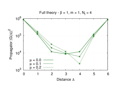
Figure 2: The propagator at different values of $\mu$.

We define the propagator at finite temperature $T=N_{t}^{-1}$ and chemical potential $\mu$ by

$$\left\langle\chi\left(t_{1}\right)\overline{\chi}\left(t_{2}\right)\right\rangle=\frac{1}{Z_{1}}\left\langle K^{-1}\left(t_{1},t_{2}\right)\right\rangle$$ (32)

with partition function $Z_{1}$ given by (21). It is helpful to introduce the notation

$$G\left(\Delta\right)=\left\langle\chi\left(1\right)\overline{\chi}\left(1+\hat{\Delta}\right)\right\rangle$$ (33)

with $\hat{\Delta}=\Delta\,\textrm{mod}\,N_{t}$. For small lattices, the inversion of the fermion matrix and the calculation of the expectation value can be done analytically. A typical example can be found in Fig. 2. For small distances the propagator $G\left(\Delta\right)$ falls off exponentially, but due to the finite lattice extension eventually rises again. The introduction of a finite chemical potential $\mu$ shifts the minimum and results in $G\left(\Delta\right)\neq G\left(-\Delta\right)$.

IV Numerical Results

IV.1 Implementation

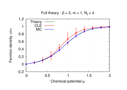
Figure 3: Typical errors estimated by the standard deviation.

In the previous section we derived numerous analytical results, which allow us to benchmark the complex Langevin evolution and check for its correctness. For the numerical simulations we implemented an adaptive numerical integration scheme of the associated Langevin equation as described in Sec. II.3. Using a computer algebra system, we can determine the inverse of the fermion matrix in (7) and find an analytical expression of the drift term in (16) for small lattices in order to minimize numerical errors.

The evaluation of the observables for a given set of parameters begins with a hot start, i.e., the random initialization of the auxiliary field, followed by typically $10^{4}$ steps for thermalization. The field configuration is then sampled about $\mathcal{O}\left(10^{5}\right)$ times and used to evaluate the observables. To reduce potential autocorrelation effects, two subsequent samples are separated by ten dummy steps. In all following plots, numerical values obtained by a complex Langevin evolution will be denoted by “CLE,” while analytical results are denoted by “Theory.”

A simple method to estimate the error is to take the standard deviation of the different samples of a given observable in a particular run. However, the resulting errors are much larger than the empirical observed statistical fluctuations between different runs and are overestimated, see Fig. 3 for a typical example. In order to obtain more reliable error bounds, we employ a bootstrap analysis DeGrand and Detar (2006). Besides the statistical error, we also have to deal with systematic errors induced by a finite stepsize. To this end we checked that the stepsize parameter $\delta$ in (17) is sufficiently small.

As an additional test we used an adaptive quasi-Monte Carlo strategy Morokoff and Caflisch (1995) for the direct evaluation of expectation values, which works well for sufficiently small $N_{t}$ and $\mu$. On larger lattices the sign problem is severe and the algorithm fails. As the path integral measure falls off rapidly for large field configurations, we replace the numerically difficult noncompact integration over the auxiliary field by a compact domain $\left[-\Lambda,\Lambda\right]^{N_{t}}$. We parametrize this ad hoc cutoff $\Lambda$ by

$$\Lambda=\sqrt{\frac{2\sigma}{\mathcal{N}\beta}}.$$ (34)

If the geometric mean of the field configuration is $\Lambda$, then the path integral measure is dampened by a factor of $\exp\left(-\sigma\right)$. If we choose $\sigma$ too small, we introduce a large cutoff effect. If $\sigma$ is very large, we still have the problem that the integrand is close to zero in most of the integration region. As a compromise here we use $\sigma=10$. In figures, we refer to numerical results obtained by this method as “MC.”

IV.2 Comparison of results

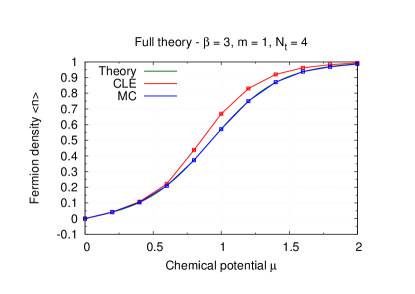
(a) Fermion density $\left\langle n\right\rangle$.

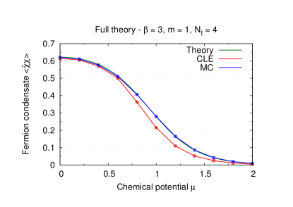
(b) Fermion condensate $\left\langle\overline{\chi}\chi\right\rangle$.

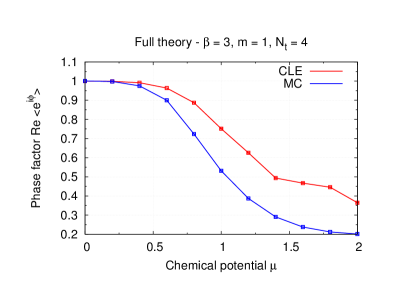
(c) Phase factor of determinant $\left\langle e^{\textrm{i}\phi}\right\rangle$.

Figure 4: Benchmarking results for $\beta=3$.

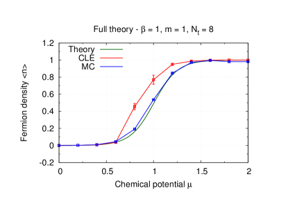
(a) Fermion density $\left\langle n\right\rangle$.

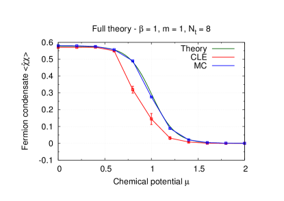
(b) Fermion condensate $\left\langle\overline{\chi}\chi\right\rangle$.

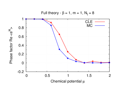
(c) Phase factor of determinant $\left\langle e^{\textrm{i}\phi}\right\rangle$.

Figure 5: Benchmarking results for $\beta=1$.

We can see the results of a typical run for two different sets of parameters in Figs. 4 and 5. Because of the high sample size, the error bars tend to be very small. We see that the results obtained with an adaptive Monte-Carlo method are in good agreement with analytical results.

The numerical results obtained with a complex Langevin evolution show some deviations for intermediate $\mu$. We systematically observe that the gap widens for decreasing values of $\beta$, i.e., stronger couplings. In addition the numerical evaluation becomes more noisy as the relative magnitude of the noise term $\eta_{t}$ increases. For large $\beta$ the agreement becomes better and the numerics are very stable.

From the phase factor of the fermion determinant, we see how the sign problem gets more severe for increasing lattice sizes. However, our approach is not affected by this. It is interesting to note that the sign problem seems to be less pronounced when using complex Langevin evolutions.

In Fig. 5 we can already see how in the limit $T\to 0$ the Silver Blaze behavior becomes apparent. In the limit $N_{t}\to\infty$ the observables will eventually become independent of the chemical potential $\mu$ up to some threshold $\mu_{c}$. It seems that the position of this onset differs slightly from analytical predictions. However, for large $\beta$ they are in good agreement.

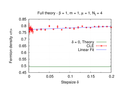
(a) Fermion density $\left\langle n\right\rangle$.

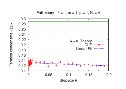
(b) Fermion condensate $\left\langle\overline{\chi}\chi\right\rangle$.

Figure 6: Extrapolation to vanishing stepsize $\delta\to 0$.

That the observed deviations are not just an effect of a finite stepsize can be seen in Fig. 6. For a typical set of parameters we calculate the fermion density and condensate for varying stepsize factors $\delta$. The extrapolation shows that also in the limit $\delta\to 0$ there is a discrepancy between theory and complex Langevin evolutions.

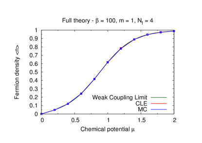
Figure 7: Density in the weak coupling regime.

IV.3 Coupling parameter dependence

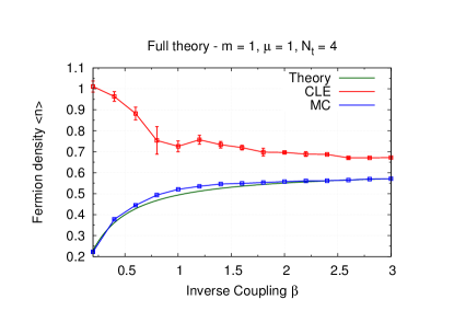
(a) Fermion density $\left\langle n\right\rangle$.

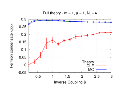
(b) Fermion condensate $\left\langle\overline{\chi}\chi\right\rangle$.

Figure 8: Observables as function of $\beta$.

In the weak coupling limit of Sec. III.3, we observe very good agreement of all numerical and analytical results. For increasing $\beta$ the numerical results are asymptotically approaching analytical results. In Figure 7 we see that for $\beta\gtrsim\mathcal{O}\left(100\right)$ the method is then able to deliver reliable results. In the XY model at finite density Aarts and James (2010b) a similar behavior was observed. For small $\beta$ the authors observed incorrect convergence, while for large $\beta$ they found agreement. However, in the XY model there is a clear separation between both regimes.

As already pointed out, the applicability of complex Langevin evolutions depend on the magnitude of $\beta$. In Figure 8 we find the density and condensate as a function of $\beta$. We observe that for weak couplings, i.e., in the limit $\beta\to\infty$, it slowly converges towards the analytical results. For $\beta=\mathcal{O}\left(100\right)$ and above we then find good agreement. Contrariwise for strong couplings we observe a large discrepancy. Moreover for $\beta\lesssim 1$ the evaluation of observables is very noisy, resulting in large error bars.

IV.4 Several flavors

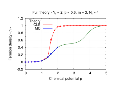
(a) Fermion density $\left\langle n\right\rangle$.

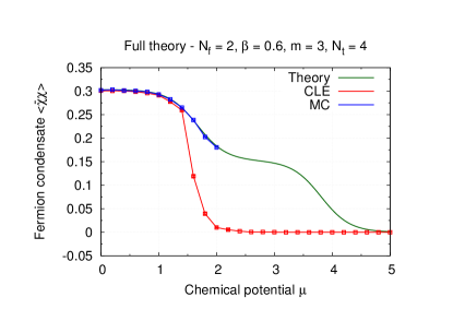
(b) Fermion condensate $\left\langle\overline{\chi}\chi\right\rangle$.

Figure 9: Observables for $\mathcal{N}=2$ degenerated flavors.

In Sec. III.2 we found that in a certain range of $\beta$, the density, the condensate and the energy density show up to $\mathcal{N}-1$ intermediate plateaus when considering $\mathcal{N}$ flavors.

We give an example for $\mathcal{N}=2$ flavors at a coupling of $\beta=0.6$ in Fig. 9. For small lattice sizes and small $\mu$ Monte Carlo studies confirm these predictions. Because of the sign problem we are restricted to $\mu\lesssim 2$ with these particular parameters, before the numerical evaluation breaks down.

When trying to reproduce the plateaus with a complex Langevin evolution, we notice that for every value of $\beta$ the result qualitatively resembles the $\mathcal{N}=1$ case. Directly after the onset the fermion density rises until it reaches saturation. Only in the limit of large $\beta$ the plateaus disappear in the analytical solution and there is agreement with numerical results.

IV.5 Analyticity at $\mu^{2}=0$

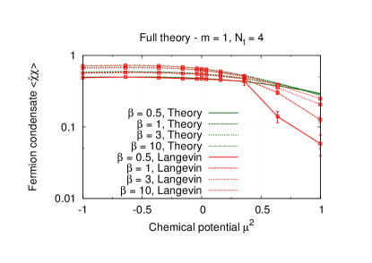
Figure 10: Logarithmic plot of $\left\langle\overline{\chi}\chi\right\rangle$ over $\mu^{2}$.

As described in Sec. III.4, we check for possible nonanalytic behavior of the condensate $\left\langle\overline{\chi}\chi\right\rangle$ at $\mu^{2}=0$. In Fig. 10 we see that for $\mu^{2}\leq 0$ the real Langevin evolution is, as expected, in agreement with theory. Because of the absence of a sign problem numerical results are reliable in this regime. Also for small $\mu^{2}\gtrsim 0$ there is no statistically significant deviation. Hence the condensate $\left\langle\overline{\chi}\chi\right\rangle$ is analytic within our numerical accuracy.

If we increase $\mu$ further, we observe that at some point a disagreement becomes apparent. The resulting gap is more pronounced for small $\beta$. It does not appear suddenly, but develops smoothly and is visible for all nonlarge $\beta$.

IV.6 Consistency conditions

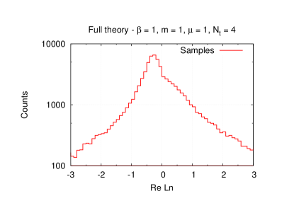
(a) Histogram of $\left\langle Ln\right\rangle$.

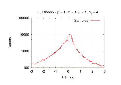
(b) Histogram of $\left\langle L\overline{\chi}\chi\right\rangle$.

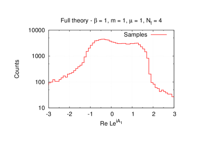
(c) Histogram of $\left\langle L\mathcal{O}\left(1,1\right)\right\rangle$.

Figure 11: Histograms for different consistency conditions.

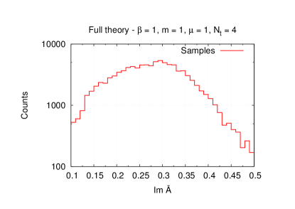
Figure 12: Distribution of $\left\langle\operatorname{Im}\overline{A}\right\rangle$.

We checked the consistency conditions of Sec. III.5 for the density $\left\langle n\right\rangle$, the condensate $\left\langle\overline{\chi}\chi\right\rangle$, and $\mathcal{O}\left(t=1,k\right)$ for different sets of parameters at $\delta=10^{-3}$. Before we begin with the interpretation of the consistency conditions, we point out again the problem of using the standard deviation to estimate error bounds. The resulting error is much larger than the actual observed statistical fluctuations and typically we obtain results like e.g. $\operatorname{Re}\left\langle L\mathcal{O}\left(1,1\right)\right\rangle=0.0152\pm 6.1221$ for $N_{t}=4$, $\mathcal{I}=0$, $\mathcal{N}=\beta=m=\mu=1$. Here $N_{t}$ denotes the temporal extension of the lattice, $\mathcal{N}$ the number of degenerated flavors, $\mathcal{I}$ the imaginary noise, $\beta$ the inverse coupling constant, $m$ the mass and $\mu$ the chemical potential. The overestimation of the error makes a meaningful interpretation of the conditions impossible. Hence we estimate the error with a bootstrap analysis.

We begin with the consistency conditions of the density and the condensate. The evaluation is extremely noisy and only becomes slightly more stable for large values of $\beta$. Without loss of generality we restrict ourselves to the case of $t=1$. As an example we quote $\operatorname{Re}\left\langle Ln\right\rangle=\left(143\pm 305\right)\times 10^{3}$ and $\operatorname{Re}\left\langle L\overline{\chi}\chi\right\rangle=\left(-52\pm 167\right)\times 10^{3}$ for $N_{t}=4$, $\mathcal{I}=0$, $\mathcal{N}=\beta=m=\mu=k=1$. The resulting expressions seem to be numerically ill-defined and despite large sample sizes, we are unable to draw any conclusions about the validity of the conditions. In our case both observables proved to be unsuitable to check for the correctness of the complex Langevin evolution.

The evaluation of the conditions for the observable $\left\langle\mathcal{O}\left(t,k\right)\right\rangle$ on the other hand is stable for all checked parameter sets. If we take the error bounds seriously, we have to conclude that some conditions are not compatible with a vanishing value and are violated. We quote here $\operatorname{Re}\left\langle L\mathcal{O}\left(t,k\right)\right\rangle=-0.1395\pm 0.0110$ for $N_{t}=4$, $\mathcal{I}=0$, $\mathcal{N}=\beta=m=k=1$, $\mu=3$ as a typical example of a violated condition and $\operatorname{Re}\left\langle L\mathcal{O}\left(t,k\right)\right\rangle=0.0061\pm 0.0208$ for $N_{t}=4$, $\mathcal{I}=0$, $\mathcal{N}=\beta=m=\mu=k=1$ as one which is compatible with a vanishing value. We also checked the conditions for $k=2,3$, which turned out to be more noisy compared to the $k=1$ case. We interpret the violated conditions as an indicator for incorrect convergence of the complex Langevin evolution.

When considering the distributions of the evaluated consistency conditions, we can gain further insights. In Fig. 11 we find histograms of $Ln$, $L\overline{\chi}\chi$, and $L\mathcal{O}\left(1,1\right)$. In general the distributions are asymmetrical and non-Gaussian. In the case of the density and condensate we saw that the distribution falls off extremely slowly and we observed values with an absolute value of up to $\mathcal{O}\left(10^{9}\right)$, resulting in a very noisy evaluation. In contrast the distribution of $L\mathcal{O}\left(1,1\right)$ falls off rapidly.

It is also interesting to check the distribution of the imaginary part of the auxiliary field itself. In the derivation of the consistency condition, one assumes that boundary terms of the field would vanish. It is then important to check that the imaginary part falls off rapidly enough. In Fig. 12 we find a typical histogram of the average imaginary part $\operatorname{Im}\overline{A}=N_{t}^{-1}\sum_{t}\operatorname{Im}A_{t}$ with $10^{5}$ samples. We see that the resulting distribution appears to be compatible with our hypothesis.

IV.7 Eigenvalues of the fermion matrix

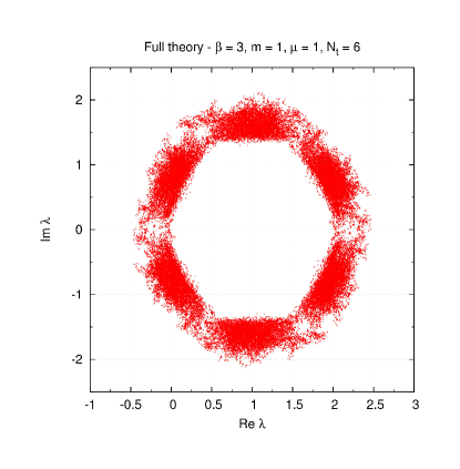
Figure 13: Eigenvalues of the fermion matrix.

In Figure 13 we find a scatter plot of the eigenvalues of the fermion matrix $K$ defined in (7). We sampled approximately $6\times 10^{4}$ eigenvalues during a complex Langevin evolution. Eigenvalues come in point-reflected pairs at point $\left(m,0\right)$, where $m$ denotes the mass of the fermion. For a vanishing chemical potential $\mu=0$ all eigenvalues lie on the line $\operatorname{Re}\lambda=m$.

IV.8 Imaginary noise

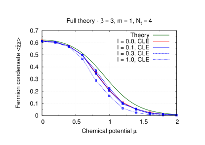
Figure 14: Condensate $\left\langle\overline{\chi}\chi\right\rangle$ with imaginary noise $\mathcal{I}$.

Assuming correct convergence of the complex Langevin evolution, observables should turn out independent of the imaginary noise term controlled by $\mathcal{I}$. However, in Fig. 14 we actually observe such a dependence. This was observed previously in other systems too Aarts et al. (2011a). Attempts to fine-tune $\mathcal{I}$ so that the complex Langevin evolution is deformed and correctly reproduces analytical results did not succeed. In almost all cases an imaginary noise $\mathcal{I}>0$ caused a more severe disagreement between numerical and analytical results.

IV.9 Periodic continuation of the imaginary part

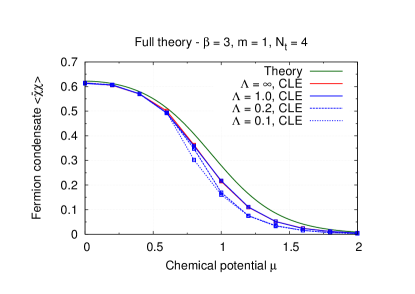
Figure 15: Condensate $\left\langle\overline{\chi}\chi\right\rangle$ with periodic cutoff $\Lambda$.

A necessary condition for the correctness of the complex Langevin evolution is that the distributions of the imaginary parts of the fields have to fall off rapidly enough. Although in the generalized Thirring model this seems to be the case, we can restrict the imaginary part of the field to the interval $\left[-\Lambda,+\Lambda\right]$ and make a periodic continuation. A similar approach was employed in Aarts et al. (2011a) (see also Aarts et al. (2010a)), where a fine-tuning of the cutoff enabled simple toy models to reproduce correct results. However, in Fig. 15 we see that every finite value of $\Lambda$ widens the gap to the correct results. Hence in this simple form this approach cannot be applied to the generalized Thirring model.

V Conclusions

In this paper we applied a complex Langevin evolution to a generalized Thirring model in $0+1$ dimensions in order to deal with the resulting sign problem for $\mu>0$. For intermediate values of the chemical potential we found a gap between analytical and numerical results, which size depends on the inverse coupling $\beta$. While for small $\beta$ the discrepancy is large, we observe agreement for large $\beta$. In particular, for $\beta\gtrsim\mathcal{O}\left(100\right)$ we are usually able to reproduce analytical results with high accuracy. Furthermore for small $\mu\gtrsim 0$ we did not observe any significant deviations to theoretical predictions and the fermion condensate is analytic at $\mu^{2}=0$.

However, in the case of more than one flavor we observed a qualitative disagreement. Our approach seems to be unable to reproduce the plateaus we found for certain ranges of $\beta$. Another interesting observation is the violation of several consistency conditions, indicating that the complex Langevin evolution might not converge correctly in general. Attempts to force correct convergence by an ad hoc fine-tuning of a periodic cutoff $\Lambda$ or an imaginary noise term $\mathcal{I}$ did not succeed.

In a subsequent paper, we will present our findings for the generalized Thirring model in $2+1$ dimensions Pawlowski and Zielinski (2013). Further investigations have to deal with the question of how to address the aforementioned problems. In particular, coordinate transformations as suggested in Aarts et al. (2013) and gauge cooling procedures like the one employed in Seiler et al. (2012) might allow a stabilization of the complex Langevin evolution.

Appendix: Plateaus

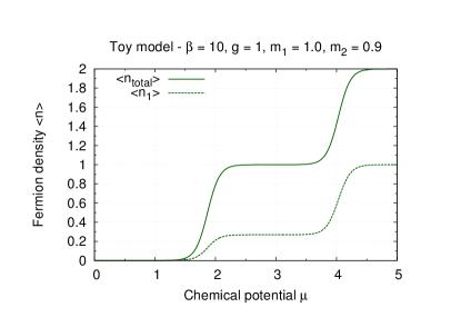
Figure 16: Densities in the toy model.

As previously discussed, in the case of $\mathcal{N}>1$ flavors we observe intermediate plateaus in the considered observables. In the nonlinear O(2) sigma model, the authors of Banerjee and Chandrasekharan (2010) found similar structures. They explained this finite size behavior with the crossing of energy levels at finite chemical potential. However, here we reproduce them with the help of a continuum model, which corresponds to the $0+1$ dimensional generalized Thirring model. To this end we consider the Hamiltonian

$$H=\sum_{i=1}^{N_{f}}m_{i}\left(n_{i}+\overline{n}_{i}\right)+g^{2}\left(\sum_{i=1}^{N_{f}}Q_{i}\right)^{2}$$ (35)

with flavor index $i=1,\dots,N_{f}$ and bare masses $m_{i}$. We introduced $Q_{i}\equiv n_{i}-\overline{n}_{i}$, the particle number operator $n_{i}=a_{i}^{\dagger}a_{i}$ and the antiparticle number operator $\overline{n}_{i}=b_{i}^{\dagger}b_{i}$, which are given in terms of ladder operators. From the grand canonical partition function

$$Z=\operatorname{Tr}\exp\left[-\beta_{T}\left(H-\sum_{i}\mu_{i}Q_{i}\right)\right]$$ (36)

with $\beta_{T}=T^{-1}$ and temperature $T$, we can derive the fermion densities

$$\left\langle n\right\rangle_{i}=\frac{1}{\beta_{T}}\frac{\partial\log Z}{\partial\mu_{i}},\quad\left\langle n\right\rangle_{\textrm{total}}=\sum_{i}\left\langle n\right\rangle_{i}.$$ (37)

The plateaus are a result of the competition between the $Q_{i}$ and $Q_{i}^{2}$ terms. A typical plot for $N_{f}=2$ can be found in Fig. 16. Like in the Thirring model they appear for intermediate values of $g^{2}$ and eventually disappear in the limit of small and large values.

References

- de Forcrand (2009) P. de Forcrand, PoS LAT2009, 010 (2009), arXiv:1005.0539 [hep-lat] .
- Lombardo (2007) M. P. Lombardo, Mod.Phys.Lett. A22, 457 (2007), arXiv:hep-lat/0509180 [hep-lat] .
- Karsch et al. (2011) F. Karsch, B.-J. Schaefer, M. Wagner, and J. Wambach, Phys.Lett. B698, 256 (2011), arXiv:1009.5211 [hep-ph] .
- Lombardo (2006) M. P. Lombardo, PoS CPOD2006, 003 (2006), arXiv:hep-lat/0612017 [hep-lat] .
- Schmidt et al. (2012) A. Schmidt, Y. D. Mercado, and C. Gattringer, PoS LATTICE2012, 098 (2012), arXiv:1211.1573 [hep-lat] .
- Mercado et al. (2013) Y. D. Mercado, C. Gattringer, and A. Schmidt, Comput.Phys.Commun. 184, 1535 (2013), arXiv:1211.3436 [hep-lat] .
- Alexandru et al. (2005) A. Alexandru, M. Faber, I. Horvath, and K.-F. Liu, Phys.Rev. D72, 114513 (2005), arXiv:hep-lat/0507020 [hep-lat] .
- Alexandru and Wenger (2011) A. Alexandru and U. Wenger, Phys.Rev. D83, 034502 (2011), arXiv:1009.2197 [hep-lat] .
- Parisi and Wu (1981) G. Parisi and Y. Wu, Sci.Sin. 24, 483 (1981).
- Damgaard and Huffel (1987) P. H. Damgaard and H. Huffel, Phys.Rept. 152, 227 (1987).
- Parisi (1983) G. Parisi, Phys.Lett. B131, 393 (1983).
- Karsch and Wyld (1985) F. Karsch and H. W. Wyld, Phys.Rev.Lett. 55, 2242 (1985).
- Aarts and James (2012) G. Aarts and F. A. James, JHEP 1201, 118 (2012), arXiv:1112.4655 [hep-lat] .
- Bilic et al. (1988) N. Bilic, H. Gausterer, and S. Sanielevici, Phys.Rev. D37, 3684 (1988).
- Aarts and Stamatescu (2008) G. Aarts and I.-O. Stamatescu, JHEP 0809, 018 (2008), arXiv:0807.1597 [hep-lat] .
- Aarts and Splittorff (2010) G. Aarts and K. Splittorff, JHEP 1008, 017 (2010), arXiv:1006.0332 [hep-lat] .
- Aarts (2009a) G. Aarts, Phys.Rev.Lett. 102, 131601 (2009a), arXiv:0810.2089 [hep-lat] .
- Aarts (2009b) G. Aarts, JHEP 0905, 052 (2009b), arXiv:0902.4686 [hep-lat] .
- Berges et al. (2007) J. Berges, S. Borsanyi, D. Sexty, and I.-O. Stamatescu, Phys.Rev. D75, 045007 (2007), arXiv:hep-lat/0609058 [hep-lat] .
- Berges and Sexty (2008) J. Berges and D. Sexty, Nucl.Phys. B799, 306 (2008), arXiv:0708.0779 [hep-lat] .
- Berges and Stamatescu (2005) J. Berges and I.-O. Stamatescu, Phys.Rev.Lett. 95, 202003 (2005), arXiv:hep-lat/0508030 [hep-lat] .
- Aarts and James (2010a) G. Aarts and F. A. James, JHEP 1008, 020 (2010a), arXiv:1005.3468 [hep-lat] .
- Ambjorn et al. (1986) J. Ambjorn, M. Flensburg, and C. Peterson, Nucl.Phys. B275, 375 (1986).
- Hamber and Ren (1985) H. W. Hamber and H. Ren, Phys.Lett. B159, 330 (1985).
- Flower et al. (1986) J. Flower, S. W. Otto, and S. Callahan, Phys.Rev. D34, 598 (1986).
- Ilgenfritz (1986) E.-M. Ilgenfritz, Phys.Lett. B181, 327 (1986).
- Aarts (2012) G. Aarts, PoS LATTICE2012, 017 (2012), arXiv:1302.3028 [hep-lat] .
- Aarts (2009c) G. Aarts, PoS LAT2009, 024 (2009c), arXiv:0910.3772 [hep-lat] .
- Aarts et al. (2010a) G. Aarts, E. Seiler, and I.-O. Stamatescu, Phys.Rev. D81, 054508 (2010a), arXiv:0912.3360 [hep-lat] .
- Aarts et al. (2011a) G. Aarts, F. A. James, E. Seiler, and I.-O. Stamatescu, Eur.Phys.J. C71, 1756 (2011a), arXiv:1101.3270 [hep-lat] .
- Aarts et al. (2011b) G. Aarts, F. A. James, E. Seiler, and I.-O. Stamatescu, PoS LATTICE2011, 197 (2011b), arXiv:1110.5749 [hep-lat] .
- Spielmann (2010) D. Spielmann, Aspects of confinement in QCD from lattice simulations, Ph.D. thesis, Ruprecht–Karls–Universität Heidelberg (2010).
- Pawlowski and Zielinski (2013) J. M. Pawlowski and C. Zielinski, Phys.Rev. D87, 094509 (2013), arXiv:1302.2249 [hep-lat] .
- Gies and Janssen (2010) H. Gies and L. Janssen, Phys.Rev. D82, 085018 (2010), arXiv:1006.3747 [hep-th] .
- Chandrasekharan and Li (2012) S. Chandrasekharan and A. Li, Phys.Rev.Lett. 108, 140404 (2012), arXiv:1111.7204 [hep-lat] .
- Thirring (1958) W. E. Thirring, Annals Phys. 3, 91 (1958).
- Christofi et al. (2007) S. Christofi, S. Hands, and C. Strouthos, Phys.Rev. D75, 101701 (2007), arXiv:hep-lat/0701016 [hep-lat] .
- Coleman (1975) S. R. Coleman, Phys.Rev. D11, 2088 (1975).
- Benfatto et al. (2009) G. Benfatto, P. Falco, and V. Mastropietro, Commun.Math.Phys. 285, 713 (2009), arXiv:0711.5010 [hep-th] .
- Itoh et al. (1995) T. Itoh, Y. Kim, M. Sugiura, and K. Yamawaki, Prog.Theor.Phys. 93, 417 (1995), arXiv:hep-th/9411201 [hep-th] .
- Cohen (2003) T. D. Cohen, Phys.Rev.Lett. 91, 222001 (2003), arXiv:hep-ph/0307089 [hep-ph] .
- Splittorff and Verbaarschot (2007) K. Splittorff and J. J. M. Verbaarschot, Phys.Rev.Lett. 98, 031601 (2007), arXiv:hep-lat/0609076 [hep-lat] .
- Kogut and Susskind (1975) J. B. Kogut and L. Susskind, Phys.Rev. D11, 395 (1975).
- Banks et al. (1976) T. Banks, L. Susskind, and J. B. Kogut, Phys.Rev. D13, 1043 (1976).
- Banks et al. (1977) T. Banks et al. (Cornell-Oxford-Tel Aviv-Yeshiva Collaboration), Phys.Rev. D15, 1111 (1977).
- Susskind (1977) L. Susskind, Phys.Rev. D16, 3031 (1977).
- Hasenfratz and Karsch (1983) P. Hasenfratz and F. Karsch, Phys.Lett. B125, 308 (1983).
- Del Debbio and Hands (1996) L. Del Debbio and S. Hands, Phys.Lett. B373, 171 (1996), arXiv:hep-lat/9512013 [hep-lat] .
- Han and Stephanov (2008) J. Han and M. A. Stephanov, Phys.Rev. D78, 054507 (2008), arXiv:0805.1939 [hep-lat] .
- Andersen et al. (2010) J. O. Andersen, L. T. Kyllingstad, and K. Splittorff, JHEP 1001, 055 (2010), arXiv:0909.2771 [hep-lat] .
- Chang (1987) C. C. Chang, Math. Comp. 49, 523 (1987).
- Ambjorn and Yang (1985) J. Ambjorn and S. K. Yang, Phys.Lett. B165, 140 (1985).
- Aarts et al. (2010b) G. Aarts, F. A. James, E. Seiler, and I.-O. Stamatescu, Phys.Lett. B687, 154 (2010b), arXiv:0912.0617 [hep-lat] .
- Molinari (2008) L. G. Molinari, Linear Algebra and its Applications 429, 2221 (2008).
- DeGrand and Detar (2006) T. DeGrand and C. E. Detar, Lattice methods for quantum chromodynamics (World Scientific, 2006).
- Morokoff and Caflisch (1995) W. J. Morokoff and R. E. Caflisch, Journal of Computational Physics 122, 218 (1995).
- Aarts and James (2010b) G. Aarts and F. A. James, PoS LATTICE2010, 321 (2010b), arXiv:1009.5838 [hep-lat] .
- Aarts et al. (2013) G. Aarts, F. A. James, J. M. Pawlowski, E. Seiler, D. Sexty, et al., JHEP 1303, 073 (2013), arXiv:1212.5231 [hep-lat] .
- Seiler et al. (2012) E. Seiler, D. Sexty, and I.-O. Stamatescu, (2012), arXiv:1211.3709 [hep-lat] .
- Banerjee and Chandrasekharan (2010) D. Banerjee and S. Chandrasekharan, Phys.Rev. D81, 125007 (2010), arXiv:1001.3648 [hep-lat] .