The GALEX Time Domain Survey I. Selection and Classification of Over a Thousand UV Variable Sources

Abstract

We present the selection and classification of over a thousand ultraviolet (UV) variable sources discovered in $\sim$ 40 deg² of GALEX Time Domain Survey (TDS) $NUV$ images observed with a cadence of 2 days and a baseline of observations of $\sim 3$ years. The GALEX TDS fields were designed to be in spatial and temporal coordination with the Pan-STARRS1 Medium Deep Survey, which provides deep optical imaging and simultaneous optical transient detections via image differencing. We characterize the GALEX photometric errors empirically as a function of mean magnitude, and select sources that vary at the 5$\sigma$ level in at least one epoch. We measure the statistical properties of the UV variability, including the structure function on timescales of days and years. We report classifications for the GALEX TDS sample using a combination of optical host colors and morphology, UV light curve characteristics, and matches to archival X-ray, and spectroscopy catalogs. We classify 62% of the sources as active galaxies (358 quasars and 305 active galactic nuclei), and 10% as variable stars (including 37 RR Lyrae, 53 M dwarf flare stars, and 2 cataclysmic variables). We detect a large-amplitude tail in the UV variability distribution for M-dwarf flare stars and RR Lyrae, reaching up to $|\Delta m|=4.6$ mag and 2.9 mag, respectively. The mean amplitude of the structure function for quasars on year timescales is 5 times larger than observed at optical wavelengths. The remaining unclassified sources include UV-bright extragalactic transients, two of which have been spectroscopically confirmed to be a young core-collapse supernova and a flare from the tidal disruption of a star by dormant supermassive black hole. We calculate a surface density for variable sources in the UV with $NUV<23$ mag and $|\Delta m|>0.2$ mag of $\sim$ 8.0, 7.7, and 1.8 deg^-2 for quasars, AGNs, and RR Lyrae stars, respectively. We also calculate a surface density rate in the UV for transient sources, using the effective survey time at the cadence appropriate to each class, of $\sim 15$ and $52$ deg^-2 yr^-1 for M dwarfs and extragalactic transients, respectively.

1. Introduction

Unlike the optical, X-ray, and $\gamma$-ray sky, which have been systematically studied in the time domain in the search for supernovae (SNe) and gamma-ray bursts (GRBs), the wide-field UV time domain is a relatively unexplored parameter space. The launch of the GALEX satellite with its 1.25 deg diameter field of view, and limiting sensitivity per 1.5 ks visit of $\sim$23 mag in the $FUV$ ($\lambda_{\rm eff}=1539$ Å) and $NUV$ ($\lambda_{\rm eff}=2316$ Å) (Martin et al., 2005; Morrissey et al., 2007), enabled the discovery of UV variable sources in repeated observations over hundreds of square degrees for the first time.

The UV waveband is particularly sensitive to hot ($\approx 10^{4}$ K) thermal emission from such transient and variable phenomena as young core-collapse SNe, the inner regions of the accretion flow around accreting supermassive black holes (SMBHs), and the flaring states of variable stars. The characterstic timescales of variables and transients in the UV range from minutes to years. M dwarf flare stars have strong magnetic activity that manifests itself in flares of thermal UV emission on the timescale of minutes (Kowalski et al., 2009). RR Lyrae stars have periodic pulsations which drive temperature fluctuations from $\sim 6000$ to 8000 K that cause periodic variability in the UV on a timescale of $\sim 0.5$ d (Wheatley et al., 2012). Core-collapse supernovae (SNe) remain bright in the UV for hours up to several days following shock breakout, depending on the radius of the progenitor star (Nakar & Sari, 2010; Rabinak & Waxman, 2011), and the presence of a dense wind (Ofek et al., 2010; Chevalier & Irwin, 2011; Svirski et al., 2012). Active galactic nuclei (AGN) and quasars demonstrate stronger variability with decreasing wavelength and longer timescales of years (Vanden Berk et al., 2004).

UV variability studies of GALEX data observed as part of the All-Sky, Medium, and Deep Imaging baseline mission surveys (AIS, MIS, DIS) from 2003 to 2007, yielded the detection of M-dwarf flare stars (Welsh et al., 2007), RR Lyrae stars, AGN, and quasars (Welsh et al., 2005; Wheatley et al., 2008; Welsh et al., 2011), and flares from the tidal disruption of stars around dormant supermassive black holes (Gezari et al., 2006, 2008a, 2009). Serendipitous overlap of 4 GALEX DIS fields with the optical CFHT Supernova Legacy Survey, enabled the extraction of simultaneous optical light curves from image differencing for 2 of the tidal disruption event (TDE) candidates (Gezari et al., 2008a), and enabled the association of transient UV emission with two Type IIP supernovae (SNe) within hours of shock breakout (Schawinski et al., 2008; Gezari et al., 2008b). Chance overlap of GALEX observations with the survey area of the optical Palomar Transient Factory (PTF) detected a Type IIn SN whose rising UV emission over a few days was interpreted as a delayed shock breakout through a dense circumstellar medium (Ofek et al., 2010).

Motivated by the promising results from the analysis of random repeated GALEX observations, and the demonstrated value of overlap with optical time domain surveys, we initiated a dedicated GALEX Time Domain Survey (TDS) to systematically study UV variability on timescales of days to years with multiple epochs of $NUV$ images observed with a regular cadence of 2 days. The GALEX TDS fields were selected to overlap with the Pan-STARRS1 Medium Deep Survey (PS1 MDS) (Kaiser et al., 2010). GALEX TDS and PS1 MDS are well-matched in field of view, sensitivity, and cadence (shown in Table 1). Here we present the analysis of 42 GALEX TDS fields which intersect with the PS1 MDS footprint, for a total area on the sky of 39.91 deg², which were monitored over a baseline of 3.32 years (February 2008 $-$ June 2011). In this paper we use PS1 MDS deep stack catalogs to characterize the optical hosts of GALEX TDS sources. Simultaneous UV and optical variability of GALEX TDS sources culled from matches with the PS1 transient alerts (Huber et al., 2011) will be presented in future papers.

The paper is structured as follows. In §2 we describe the GALEX TDS survey design, and in §3 we describe our statistical methods for selecting UV-variable sources and characterizing their UV variability. In §4 we describe the multiwavelength catalog data used to identify the hosts of the UV-variable sources, including archival optical data, a deep PS1 MDS catalog, and archival redshift and X-ray catalogs. In §5 we describe our sequence of steps for classifying the GALEX TDS sources, in §6 we summarize our classification results, and the UV variability properties of our classified sources. In §7 we conclude with implications for future surveys.

2. GALEX TDS Observations

GALEX TDS monitored 6 out of 10 total PS1 MDS fields, with 7 GALEX TDS pointings (labeled PS_fieldname_MOSpointing) at a time to cover the PS1 7 deg² field of view. During the window of observing visibility of each GALEX TDS field (from $2-4$ weeks, $1-2$ times per year), they were observed with a cadence of 2 days, and a typical exposure time per epoch of 1.5 ks (or a 5$\sigma$ point-source limit of $m_{AB}\sim 23.3$ mag), with a range from 1.0 to 1.7 ks. The $NUV$ detector developed a problem on 2010 May 4 during observations of PS_ELAISN1, and so we do not include epochs observed between this time and when the the instrument was fixed on 2010 June 23 in our analysis. Figure 1 shows the position of the GALEX TDS fields relative to the PS1 MDS fields, and Table 2 lists the R.A. and Dec of their centers, the Galactic extinction ($E(B-V)$) for each field from the Schlegel et al. (1998) dust maps, and the number of epochs per field. The median number of epochs per field is 24. PS_CDFS_MOS00 is an exception with 114 epochs, because it was monitored with a rapid cadence ($|\Delta t|\sim 3$ hours) over a period of 10 days in 2010 November. Some offsets in the GALEX pointings from the footprint of the PS1 MDS fields were necessary in order to avoid UV-bright stars in the field of view that would violate the detector’s bright-source count limits.

Figure 2 shows the temporal sampling of GALEX TDS observations in the $NUV$ in comparison to the PS1 MDS observations in the $g_{\rm P1}$, $r_{\rm P1}$, $i_{\rm P1}$, $z_{\rm P1}$, and $y_{\rm P1}$ bands from February 2008 to June 2011. PS1 began taking commissioning data of the MDS fields in May 2009, but did not begin full survey operations until a year later. The GALEX $FUV$ detector became non-operational in May 2009, and so we only include $NUV$ images in our study.

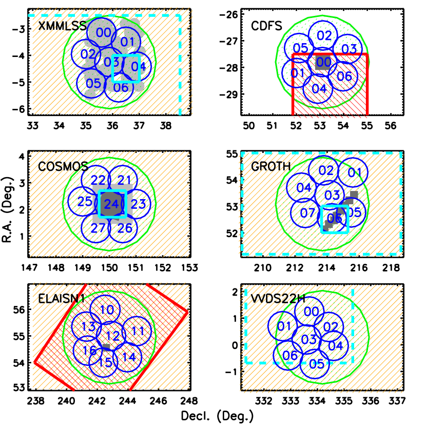
Figure 1.— GALEX TDS $1.1\deg$ diameter field pointings shown in blue, and the PS1 MDS $3.5\deg$ diameter field pointings shown in green. Orange hatched regions show the coverage of SDSS in the optical, red hatched regions shows the coverage of SWIRE in the optical, and cyan rectangles indicate the coverage of the CFHTLS Deep (solid lines) and Wide (dashed lines) surveys in the optical. Light grey regions show the coverage of XMM-Newton X-ray observations, and dark grey regions show the coverage of Chandra X-ray observations.

Figure 2.— Dates of GALEX TDS $NUV$ observations compared to PS1 MDS observations in the $g_{\rm P1}$, $r_{\rm P1}$, $i_{\rm P1}$, $z_{\rm P1}$, and $y_{\rm P1}$ bands. Dotted lines show yearly intervals.

3. Statistical Measurements

3.1. Selection of Variable Sources

Since most galaxies are unresolved by the GALEX $NUV$ 5.3 arcsec full-width at half-maximum (FWHM) point spread function (PSF), we can use simple aperture photometry instead of image differencing to measure variability. We create a master list of unique source positions from the pipeline-generated catalogs (Morrissey et al., 2007) for all the individual epochs, as well as deep stacks of all the epochs, using a clustering radius of 5 arcsec. This radius is chosen such that for the typical astrometry error of GALEX of $0\farcs 5$, the Bayesian probability that the match is real is larger than the Bayesian probability that the match is spurious (Budavári & Szalay, 2008). The final master list includes 419,152 sources.

In order to select intrinsically variable sources in our survey, we first need to characterize the photometric errors. Although the GALEX images are Poisson-limited, the Poisson error underestimates the total error in the GALEX catalog magnitudes by a factor of $\sim 2$ (Trammell et al., 2007). This discrepancy is attributed to systematic errors such as uncertainties in the detector background and flat-field. Thus, we measure the photometric error empirically by calculating the standard deviation of aperture magnitudes in bins of mean magnitude, $\langle m\rangle$. We only include objects in the pipeline-generated catalogs that are detected in all or $\geq$10 epochs. In each bin of $N$ objects with $\langle m\rangle_{i}=(\sum_{k=1}^{n}m_{i,k})/n$ (each bin typically has $N$ = 50 to 1000 sources), we calculate for each epoch $k$ of a total of $n$ epochs,

$$\sigma(\langle m\rangle,k)=\sqrt{\frac{1}{N-1}\sum_{i=1}^{N}(m_{i,k}-\langle m\rangle_{i})^{2}}$$ (1)

where $m_{i,k}$ is the magnitude (in the AB system) given by $m_{i,k}=-2.5\log(f_{6})+zp+C_{\rm ap}-8.2E(B-V)$, $f_{6}$ is the background-subtracted flux in a 6 arcsec radius aperture, $zp$ = 20.08, the aperture correction is $C_{\rm ap}=-0.23$ mag (Morrissey et al., 2007), and we correct for Galactic extinction using the values for $E(B-V)$ listed in Table 2. We use 3$\sigma$ clipping to remove outliers in the calculation of $\sigma(\langle m\rangle,k)$ which can arise from artifacts.

The astrometric precision depends on the signal-to-noise of the source, thus we also empirically measure a magnitude-dependent clustering radius. We do so by measuring the cumulative distribution of spatial separations between the position in each epoch and the mean position for sources in bins of $\langle m\rangle$, and record $d_{95}(\langle m\rangle,k)$, the value for which 95% of sources have a separation less than or equal to that value. The resulting value for $d_{95}$ is a strong function magnitude, increasing from $\sim$ 1 arcsec for $\langle m\rangle=18.0$ mag to $\sim$ 4 arcsec for $\langle m\rangle=23.0$ mag. Figures 3 and 4 show $\sigma(\langle m\rangle,k)$ and $d_{95}(\langle m\rangle,k)$ for an example GALEX TDS field PS_COSMOS_MOS23, a quadratic fit to the median function for all epochs in that field, and the median function fit over all fields.

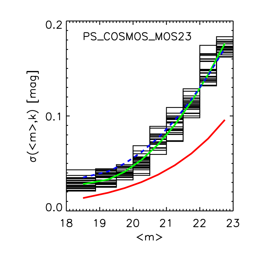
Figure 3.— Empirical determination of 1$\sigma$ photometric errors as a function of mean magnitude from the standard deviation of sources detected by the pipeline catalogs in $\geq$ 10 epochs for one of the GALEX TDS fields PS_COSMOS_MOS23. Solid green line shows a quadratic fit to the error function for the field PS_COSMOS_MOS23, and dashed blue line shows a quadratic fit to the median error function for all of the GALEX TDS fields. Solid red line shows the expected 1$\sigma$ Poisson error, which underestimates the total photometric error by a factor of $\sim 2$.

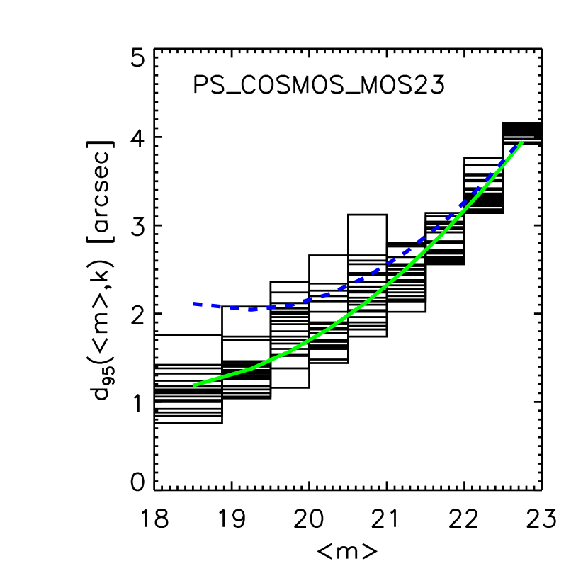
Figure 4.— Maximum spatial separation from the mean for 95% of the sources as a function of mean magnitude from the cumulative distribution of sources detected by the pipeline catalogs in $\geq$ 10 epochs for one of the GALEX TDS fields PS_COSMOS_MOS23. Solid green line shows a quadratic fit to the error function for the field PS_COSMOS_MOS23, and dashed blue line shows a quadratic fit to the median distance function for all of the GALEX TDS fields. Note that due to systematic differences in the PSF between fields, the distance function radius for PS_COSMOS_MOS23 is up to $\sim 1$ arcsec smaller than the median for all fields, since for $\langle m\rangle\ {\raise-2.15277pt\hbox{$\buildrel<\over{\sim}$}}\ 20$ mag, $d_{95}\sim 2$ arcsec in the PS_XMMLSS, PS_CDFS, PS_GROTH, and PS_ELAISN1 fields and $d_{95}\sim 3$ arcsec in the PS_VVDS22H fields.

In our master list of source positions, we include all sources detected, including sources detected in only one epoch, and fix the centroid to the epoch for which the source is detected with maximum flux. We measure forced aperture magnitudes at the positions of each source in epochs where the source was not detected by the pipeline or the spatial separation of the matched source is greater than $d_{95}(\langle m\rangle,k)$. When the aperture magnitude is fainter than $m_{\rm lim}$ in an epoch, it is flagged as an upper limit and replaced with $m_{\rm lim}$, where $m_{\rm lim}=-2.5\log(5\sqrt{(B_{\rm sky}N_{\rm pix}/T_{\rm exp})}+zp+C_{\rm ap}$, where $B_{\rm sky}=3\times 10^{-3}$ counts s^-1 pixel^-1, $N_{\rm pix}=16\pi$ and $T_{\rm exp}$ is the exposure time of that epoch in seconds.

We select sources that have at least one epoch for which $|m_{k}-\langle m\rangle|>5\sigma(\langle m\rangle,k)$, where $\langle m\rangle$ is calculated only from epochs that have a magnitude above the detection limit of that epoch. We use this selection method to be sensitive to short-term and long-term variability, as well as transients. This 5$\sigma$ selection is quite conservative, and requires variability amplitudes increasing from $|\Delta m|>0.1$ mag for $\langle m\rangle\sim 18$ mag up to $|\Delta m|>1.0$ mag for $\langle m\rangle\sim 23$ mag.

We make the following cuts to the $5\sigma$ variable source sample to remove artifacts:

• We remove sources with pipeline artifact flags indicating window bevel reflections or ghosts from the dichroic beam splitter.

• We remove the brightest objects, with $\langle m\rangle<18.0$, due to the large area subtended by the PSF which causes uncertainty in the background subtraction.

• We select sources within a radius of $0.55$ deg of the center of the field, in order to avoid glints and PSF distortions, which are more prominent on the edges of the image, from un-corrected spatial distortions of photons recorded by the detectors.

• We do not include objects that are within 1.5 arcmin of a $m<17$ mag source, to avoid regions affected by the bright source’s PSF and ghost artifacts. Ghost artifacts can appear within $30-60$ arcsec above and below a bright source in the Y detector direction. Ghosts are point-like, and thus can only be identified from their Y detector position relative to a bright source. While ghosts do not usually appear in the GALEX pipeline catalogs, we apply this cut since our forced aperture photometry could mistake ghosts for transient sources.

• We veto objects for which in the epoch of maximum $|m_{k}-\langle m\rangle|/\sigma(\langle m\rangle,k)$ or maximum flux, the aperture flux ratio of the object has $f_{6}/f_{3.8}>R_{90}$, where $f_{6}$ is the 6.0 arcsec radius aperture flux, $f_{3.8}$ is the 3.8 arcsec radius aperture flux, and $R_{90}$ is the maximum cumulative aperture flux ratio measured for 90% of the sources in the reference source sample used to calculate $\sigma(\langle m\rangle,k)$ in that epoch. This cut removes fluctuations in the background due to reflections from bright stars just outside the field-of-view, as well as epochs where the PSF is distorted due to a degradation in resolution which sometimes occurs in the Y detector direction. This also vetoes cases when the pipeline shreds a source into multiple sources, and the source is detected as variable because the center of the aperture is off-center from the peak source flux.

• Finally, we visually inspect all of the remaining variable sources to remove any remaining artifacts that passed through the cuts above.

Figure 5 shows a gallery of good sources and vetoed variable sources from our automated cuts (for a bright reflection in panel a, an off-center source in panel b, and a likely ghost in panel c) and manual cuts (for a diffuse reflection in panel d). Our final GALEX TDS 5$\sigma$ variable sample after the cuts listed above has a total of 1078 sources.

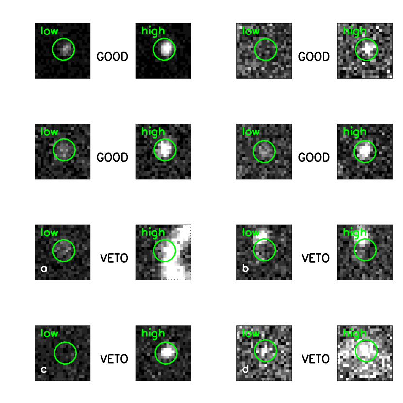
Figure 5.— Left: Gallery of good and vetoed variable sources during their epochs of minimum (“low”) and maximum (“high”) flux. Green circle shows a 6 arcsec (4 pixel) aperture radius. Sources vetoed for $f_{6}/f_{3.8}>R_{90}$ shown in panels $a$ and $b$, a source vetoed as a likely ghost within 1.5 arcmin of a $m<17$ mag source shown in panel $c$, and a manually vetoed source shown in panel $d$. For each source the grayscale is linear, and is scaled to the peak of the source in its “high” state.

3.2. Variability Statistics

We characterize the variability of each 5$\sigma$ variable UV source using several statistical measures. We measure the structure function (following di Clemente et al. (1996)),

$$V(\Delta t)=\sqrt{\frac{\pi}{2}\langle|\Delta m_{ij}|\rangle_{\Delta t}^{2}-\langle\sigma_{i}^{2}+\sigma_{j}^{2}\rangle_{\Delta t}}$$ (2)

where brackets denote averages for all pairs of points on the light curve of an individual source with $i<j$ and $t_{j}-t_{i}=\Delta t$. The 2 day cadence of the observations combined with the seasonal visibility of the fields results in a distribution of time intervals between observations (shown in Figure 6) that fall into 6 characteristic timescale bins: $\Delta t_{\rm 2d}$ = $2\pm 0.5$ d, $\Delta t_{\rm 4d}$ = $4\pm 0.5$ d, $\Delta t_{\rm 6d}$ = $6\pm 0.5$ d, $\Delta t_{\rm 8d}$ = $8\pm 0.5$ d, $\Delta t_{\rm 1yr}=0.96\pm 0.14$ yr, and $\Delta t_{\rm 2yr}=1.96\pm 0.04$ yr. We measure the structure function in these 6 bins, and define $S_{\rm d}$ to be the maximum value of the structure function evaluated for $\Delta t_{\rm 2d},\Delta t_{\rm 4d},\Delta t_{\rm 6d}$, and $\Delta t_{\rm 8d}$, and $S_{\rm yr}$ to be the maximum value of the structure function evaluated for $\Delta t_{\rm 1yr}$ and $\Delta t_{\rm 2yr}$. We also measure the intrinsic variability as defined by Sesar et al. (2007), $\sigma_{int}=\sqrt{\Sigma^{2}-\xi^{2}}$, where $\Sigma^{2}=\frac{1}{n-1}\sum_{k=1}^{n}(m_{k}-\langle m\rangle)^{2}$ and $\xi^{2}=\frac{1}{n}\sum_{k=1}^{n}\sigma(\langle m\rangle,k)^{2}$, and the maximum amplitude of variability, max($|\Delta m|$).

Figure 6.— Histogram of the time intervals between all pairs of observations for the 42 fields in GALEX TDS. Hatched regions show the time intervals over which the structure function is measured for all of the sources.

3.3. UV Light Curve

In order to flag possible transient UV events that may be associated with a SN or TDE, we differentiate between stochastic variability and flaring variability. We identify flaring UV variability as sources that show a constant flux $\geq$ 10 days before the peak of the light curve, and do not fade more than 2$\sigma$ below the faintest pre-peak magnitude (measured $\geq 10$ days before the peak). This selection criteria is tailored to the $NUV$ rise times observed in SNe (Gezari et al., 2008b; Brown et al., 2009; Gezari et al., 2010; Milne et al., 2010; Ofek et al., 2010) and TDE candidates (Gezari et al., 2006, 2008a, 2009). We define constant pre-peak flux as a light curve with a reduced $\chi_{\nu}^{2}/<3~{}(\chi^{2}_{\nu}=\sum_{k=1}^{p}(m_{k}-\langle m\rangle)^{2}/(\sigma(\langle m\rangle,k)^{2}/(n-1)$, where $n$ is the number of epochs $\geq 10$ days before the peak). For those sources for which there are only upper limits $\geq$ 10 days before the peak, $\chi^{2}_{\nu}$ is set to 1. Flaring sources with no detections before the peak are further labeled as transients. Sources with $\chi_{\nu}^{2}/\geq 3$, or that fade below 2$\sigma$ of the faintest magnitude measured $\geq 10$ days before the peak are labeled as stochastically variable. We flag 116 flares, 145 transients, 595 stochastically variable sources, and remain with 222 sources with neither light-curve classification flag. In Figure 7 we show example light curves of sources flagged as stochastically variable (’V’), flares (’F’), and transients (’T’).

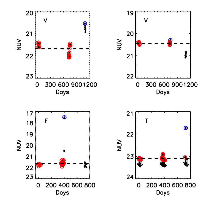
Figure 7.— Example light curves of sources flagged as stochastically variable (’V’), flares (’F’), and transient flares (’T’). Epochs $\geq 10$ days before the epoch of peak flux are circled in red, and the epoch of peak flux is circled in blue. Thick dashed line indicates the mean flux $\geq 10$ days before the peak.

4. Host Properties

4.1. Archival Optical Imaging Catalogs

We first characterize the host properties of the UV variable sources using archival optical $u$, $g$, $r$, $i$, and $z$ photometry and morphology from matches to the SDSS Photometric Catalog, Release 8 (Aihara et al., 2011) ($m_{\rm lim}\sim 22$ mag), the CFHTLS Deep Fields D1, D2, and D3 ($m_{\rm lim}\sim 26.5$ mag) and Wide Fields W1, W3, and W4 ($m_{\rm lim}\sim 25$ mag) merged catalogs version T0005 , and the SWIRE ELAIS N1 and CDFS Region catalogs ($m_{\rm lim}\sim 24$ mag) (Surace et al., 2004). For sources with matches in multiple catalogs, we use the match from the deepest catalog. We convert the CFHTLS magnitudes to the SDSS system using the conversions in Regnault et al. (2009), and the SWIRE Vega magnitudes to the SDSS system using the transformations measured for stellar objects available at the INT WFS web site . We then correct for Galactic extinction using the Schlegel et al. (1998) dust map values for $E(B-V)$ listed in Table 2. Figure 1 shows the overlap of the GALEX TDS fields with the available archival optical catalogs.

4.2. Pan-STARRS1 Medium Deep Survey

The GALEX TDS fields overlap with the PS1 MDS fields MD01 (PS_XMMLSS), MD02 (PS_CDFS), MD04 (PS_COSMOS), MD07 (PS_GROTH), MD08 (PS_ELAISN1), and MD09 (PS_VVDS22H). The Pan-STARRS1 observations are obtained through a set of five broadband filters, ($g_{\rm P1}$, $r_{\rm P1}$, $i_{\rm P1}$, $z_{\rm P1}$, and $y_{\rm P1}$). Further information on the passband shapes is described in Stubbs et al. (2010). The PS1 MD fields are observed with a typical cadence in a given filter of 3 days, with an observation in the $g_{\rm P1}$ and $r_{\rm P1}$ bands on night one, in the $i_{\rm P1}$ band on night two, and the $z_{\rm P1}$ band on night three, with $y_{\rm P1}$-band observations during each of three nights on either side of the Full Moon. Image differencing is performed on the nightly stacked images, reaching a typical 5$\sigma$ detection limit of $\sim 23.3$ mag per epoch in the $g_{\rm P1}$, $r_{\rm P1}$, $i_{\rm P1}$ bands and $\sim 21.7$ mag in the $y_{\rm P1}$ band. Image difference detections from the PS1 Image Processing Pipeline (IPP; Magnier (2006)) and an independent pipeline hosted by Harvard/CfA (Rest et al., 2005) are internally distributed to the PS1 Science Consortium as transient alerts for visual inspection and classification.

Deep stacks of the multi-epoch observations were generated to provide deep imaging with a 5$\sigma$ point-source limiting magnitude of $\sim$ 24.9, 24.7, 24.7, 24.3, 23.2 mag in the $g_{\rm P1}$, $r_{\rm P1}$, $i_{\rm P1}$, $z_{\rm P1}$, and $y_{\rm P1}$ bands, respectively, and typical seeing (PSF FWHM) of $\sim 1.4,1.3,1.0,1.0,1.0$ arcsec in the 5 bands respectively. The magnitudes are in the “natural” Pan-STARRS1 system, $m=-2.5$log(flux)+$m^{\prime}$, with a relative zeropoint adjustment $m^{\prime}$ made in each band for each individual epoch (Schlafly et al., 2012) before stacking to conform to the absolute flux calibration in the AB magnitude system (Tonry et al., 2012). We convert the PS1 magnitudes to the SDSS system using the bandpass transformations measured for stellar SEDs in Tonry et al. (2012), and correct for Galactic extinction using the Schlegel et al. (1998) dust map values for $E(B-V)$ listed in Table 2. We obtain morphology information from the PS1 IPP output parameters in the $i_{\rm P1}$ filter for the PSF magnitude (PSF_INST_MAG), the aperture magnitude (PSF_AP_MAG), and the PSF-weighted fraction of unmasked pixels PSF_QF, to define a point source or extended source as: IF PSF_INST_MAG$-$PSF_AP_MAG $<0.04$ mag AND PSF_QF $>0.85$ THEN class = pt IF PSF_INST_MAG$-$PSF_AP_MAG $>0.04$ mag AND PSF_QF $>0.85$ THEN class = ext We calibrated these parameter cuts by comparing sources detected in both the PS1 MDS and archival optical catalogs. Figure 8 shows the PS1 star/galaxy separation criteria for 110,804 sources detected in both PS1 and SDSS catalogs in the PS_GROTH field, and for 169,461 sources detected in both PS1 and CFHT catalog in the PS_GROTH field, with $i<22$ mag, the faintest magnitude for 96% of the optical hosts of the GALEX TDS sources, and the magnitude limit where all three catalogs are complete. Even though the CFHT catalogs are deeper than SDSS, they do not attempt to separate stars and galaxies for $i\ {\raise-2.15277pt\hbox{$\buildrel>\over{\sim}$}}\ 21$ mag, and classify all sources fainter than this magnitude as point sources. However, it is clear from both comparison plots, that the PS1 criterion of PSF_INST_MAG$-$PSF_AP_MAG $<0.04$ mag does an even better job of separating the locus of stars from galaxies than both catalogs down to $i\sim 22$ mag.

Figure 8.— Comparison of the star/galaxy separator used in the PS1 MD catalogs (thick dashed lines) to matches in the SDSS (left) and CFHT (right) archival catalogs in the PS_GROTH field as a function of $i$-band magnitude.

4.3. Archival Redshift and X-ray Catalogs

We also take advantage of the many archival X-ray and spectroscopic catalogs available from the overlap of the GALEX TDS survey with legacy survey fields. In the PS_CDFS field we us X-ray catalogs from the 0.3 deg² Chandra Extended CDFS survey (Giacconi et al., 2002; Lehmer et al., 2005; Virani et al., 2006), and redshift catalogs from the VIMOS VLT Deep Survey (VVDS) (Le Fèvre et al., 2004), and a compilation of redshift catalogs from GOODS and SWIRE . In the PS_XMMLSS field we use X-ray catalogs from the 5.5 deg² XMM-LSS survey (Chiappetti et al., 2005; Pierre et al., 2007), and redshift catalogs from VVDS (Le Fèvre et al., 2005). In the PS_COSMOS field, we use X-ray catalogs from the 1.9 deg² XMM-Newton Wide-Field Survey (Hasinger et al., 2007) and the 0.9 deg² Chandra COSMOS survey (Elvis et al., 2009), and redshifts from the Magellan COSMOS AGN survey (Trump et al., 2007, 2009), the VLT zCOSMOS bright catalog (Lilly et al., 2007, 2009), and the Chandra COSMOS Survey catalog (Civano et al., 2012). In the PS_GROTH field we use X-ray catalogs from the 0.67 deg²Chandra Extended Groth Strip (Nandra et al., 2005; Laird et al., 2009) and redshift catalogs from the DEEP2 Galaxy Redshift Survey (Newman et al., 2012). For PS_ELAISN1 we use the X-ray catalog from the 0.08 deg² Chandra ELAIS-N1 deep X-ray survey (Manners et al., 2003). Figure 1 shows the overlap of the GALEX TDS fields with the archival X-ray surveys. Finally, we also match the sources with the ROSAT All-Sky Bright Source and All-Sky Survey Faint Source catalogs (Voges et al., 1999, 2000).

5. Classification

We classify the GALEX TDS sources using a combination of optical host photometry and morphology, UV variability statistics, and matches with archival X-ray and redshift catalogs. Table 3 summarizes the sequence of steps we use to classify the sources, which we describe in detail below.

5.1. Cross-Match with Optical Catalogs

We first cross-matched our 1078 GALEX TDS sources with the archival $u,g,r,i,z$ catalogs described in §4.1 with a matching radius of 3 arcsec. This radius is recommended for matches between GALEX and ground-based optical catalogs (Budavári & Szalay, 2008), and corresponds to a spurious match rate of only $1-2\%$ at the high Galactic latitudes of the GALEX TDS fields (Bianchi et al., 2011). However, we found that there was a population of “orphans” (no optical match within 3 arcsec) that were detected in their $NUV$ low-state, and had a match between $3-4$ arcsec with an optically identified quasar. Given the strong likelihood that these are real matches, we increased our matching radius to 4 arcsec. We use the star/galaxy classifications from the catalogs to label sources as point sources (pt) or extended sources (ext). This results in 878/1078 optical matches (81%), with the majority of sources without matches in PS_CDFS, which is only partially covered by the archival catalogs.

We then match the sources that do not have archival optical matches to the PS1 MDS catalog described in 4.2, this increases the number of sources with optical photometry and morphology (albeit without the $u$ band) to 1057/1078 (98%). Figure 9 shows a histogram of the $r$-band magnitude of the optical hosts, and the $NUV-r$ colors of the GALEX TDS sources in their low-state. The optical hosts have a distribution that peaks at $r\sim 21$ mag, over 3 magnitudes brighter than the detection limit of PS1 MDS, and $NUV-r\sim 1$ mag. Sources not detected in their $NUV$ low-state are shown as upper limits in the $NUV-r$ color histogram, and peak at $NUV-r>2$ mag.

Figure 9.— Left: Histogram of $r$ magnitudes of optical matches. Right: Histogram of $NUV-r$ colors of optical matches for those sources detected in the $NUV$ during their low-state (solid lines), and those sources with upper limits during their low-state (dashed lines).

5.2. Orphans

We visually inspected the PS1 stack images at the locations of the 21 sources with no optical matches, and confirm that they are true orphan events. Furthermore, all of the orphans are undetected in their low-state in the $NUV$, with upper limits of $NUV>(22.3-23.1$) mag. Thus the orphan hosts are likely distant stars or faint galaxies (i.e., dwarf galaxies or high-redshift galaxies) that are undetected during their low-state in the optical and $NUV$.

5.3. Color and Morphology Cuts

We first use the color and morphology of the optical hosts to classify the GALEX TDS 5$\sigma$ UV variable sources. We define quasars as sources with optical point-source hosts with

$$u-g<0.7$$ (3)

$$-0.1<g-r<1.0$$

in order to avoid the stellar locus and white dwarfs (Richards et al., 2002). Note that this color selection can be contaminated by catacylismic variable stars (CVs), which overlap in color-color space with the quasar sample. Indeed, two of the sources classified by color as quasars are in fact spectroscopically confirmed CVs (VVDS22H_MOS05-05 and ELAISN1_MOS15-02). VVDS22H_MOS05-05 is ROTSE3 J221519.8-003257.2, a confirmed cataclysmic variables with a dwarf-nova type spectrum. We observed ELAISN1_MOS15-02 with the APO 3.5m telescope Dual Imaging Spectrograph (DIS) on 2011 May 3 and detected broad Balmer emission lines from a Galactic source, characteristic of a CV/dwarf nova spectrum. While these sources stood out easily because of their extreme magnitude of variability of $|\Delta m|>4$ mag, shown in Figure 10, there may be lower amplitude CV events that are still hiding in our quasar sample. However, given the low surface density of CVs relative to quasars in the sky (Szkody et al., 2011), the expected contamination rate is consistent with the two CVs identified.

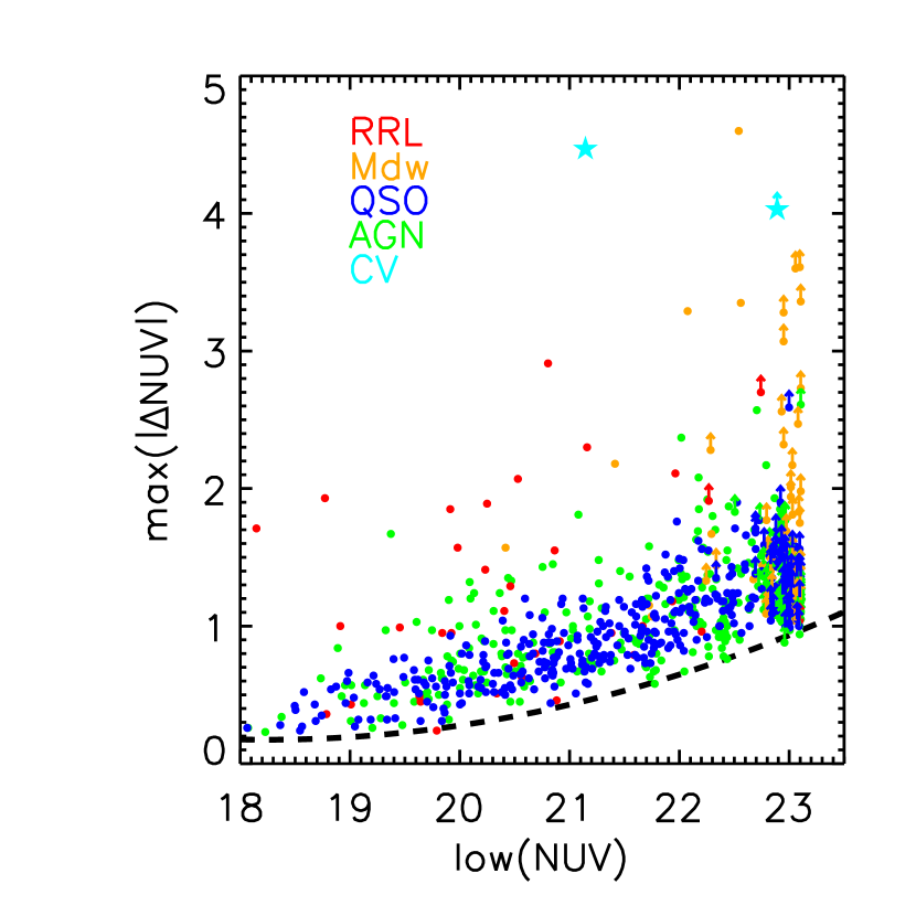
Figure 10.— Maximum $NUV$ variability amplitude as a function of low-state $NUV$ magnitude for sources classified as RR Lyrae (red), M dwarfs (yellow), quasars (blue) AGN (green), and CVs (cyan). Dashed line shows the median 5$\sigma$ error selection function used to select the variable sources.

We define RR Lyrae stars as sources with optical point source hosts with

$$0.75<u-g<1.45$$ (4)

$$-0.25<g-r<0.4$$

$$-0.2<r-i<0.2$$

$$-0.3<i-z<0.3$$

(Sesar et al., 2010). Note that the color cuts for quasars and RR Lyrae require the $u$-band, which is not available for sources with PS1-only matches. However, we define M dwarf stars as point sources with

$$r-i>0.42$$ (5)

$$i-z>0.24$$

$$g<22.2$$

$$r<22.2$$

$$i<21.3$$ (6)

(West et al., 2011), which does not require $u$-band data. We classify stars on the main stellar locus as those with

$$1.0<u-g<2.25$$ (7)

$$0.4<g-r<1.0$$

$$-0.2<r-i<2.0$$

$$-0.3<i-z<1.0$$

modified from Yanny et al. (2009). This color and morphology selection results in 37 RR Lyrae, 53 M-dwarf flare stars, 17 stars, and 325 quasars. Figure 11 shows the optical color-color diagram of the sources with optical point-source hosts and $u$-band data, and their classifications as quasars, RR Lyrae, M dwarfs, and stars.

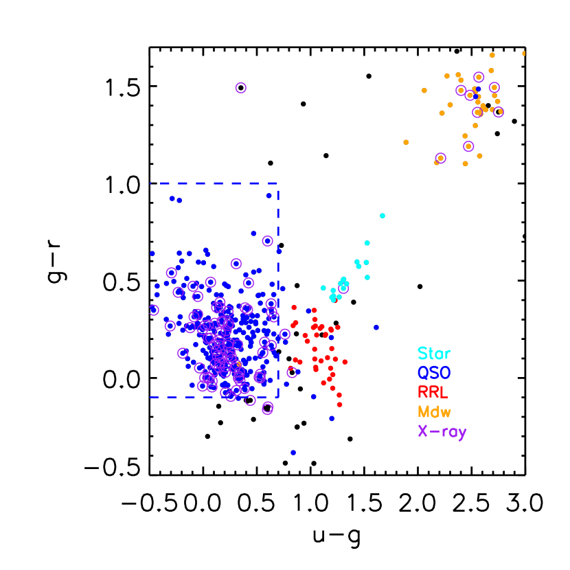
Figure 11.— Colors of archival optical matches to UV variable sources with point-like optical hosts (black points). Dashed blue line shows the region in color-color space used to define quasars from optical colors and morphology alone. Sources with classification are color coded as quasars in blue, RR Lyrae in red, and M dwarf stars in yellow, and main stellar locus stars in cyan. Sources with archival X-ray matches are circled in purple.

5.4. UV Variability Cuts

Figure 12 shows the structure function on timescales of days and years described in §3 for the sources classified as RR Lyrae and quasars in §5.3. In Figure 13 we show the ratio of the $NUV$ structure function on timescales of years to days ($S_{\rm yr}/S_{\rm d}$). While quasars demonstrate a wide range of $S_{\rm yr}/S_{\rm d}$, all RR Lyrae have $S_{\rm yr}/S_{\rm d}<3$. We use this UV variability property to relax our color constraints, and increase our photometric sample of quasars to all sources with optical point-source hosts with $S_{\rm yr}/S_{\rm d}\geq 3$. This is equivalent to a structure function power-law exponent cut of $\gamma>0.2$, where $S(\Delta t)\propto\Delta t^{\gamma}$ (Hook et al., 1994; Vanden Berk et al., 2004; Schmidt et al., 2010). This structure-function ratio selection results in the classification of another 30 quasars. Two additional sources with optical point-source hosts have archival quasar spectra, resulting in a final quasar sample of 358 . We define active galactic nuclei (AGN), as sources with optically extended hosts that show stochastic UV variability (see §3.3), have an X-ray catalog match, and/or an archival spectroscopic classification. Figure 14 shows the optical color-color diagram of the sources with optically extended hosts, and those classified as AGN. This results in a sample of 305 AGN. We also add archival spectroscopic classifications for 6 stars. This yields a total of 776/1078 (72%) sources classified as an active galaxy (quasar or AGN) or variable star.

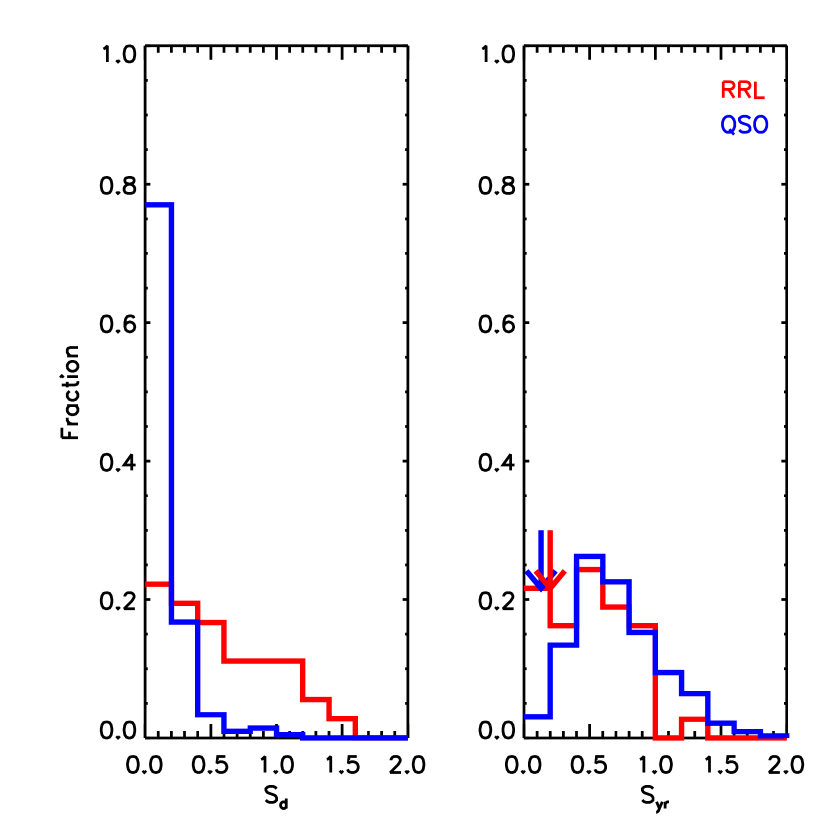
Figure 12.— Histogram of the $NUV$ structure function of sources classified as RR Lyrae (red) and quasars (blue) on a timescale of days and years. Red arrow and Blue arrow indicate the mean of S_yr measured in the SDSS $r$-band for RR Lyrae and quasars, respectively from Schmidt et al. (2010).

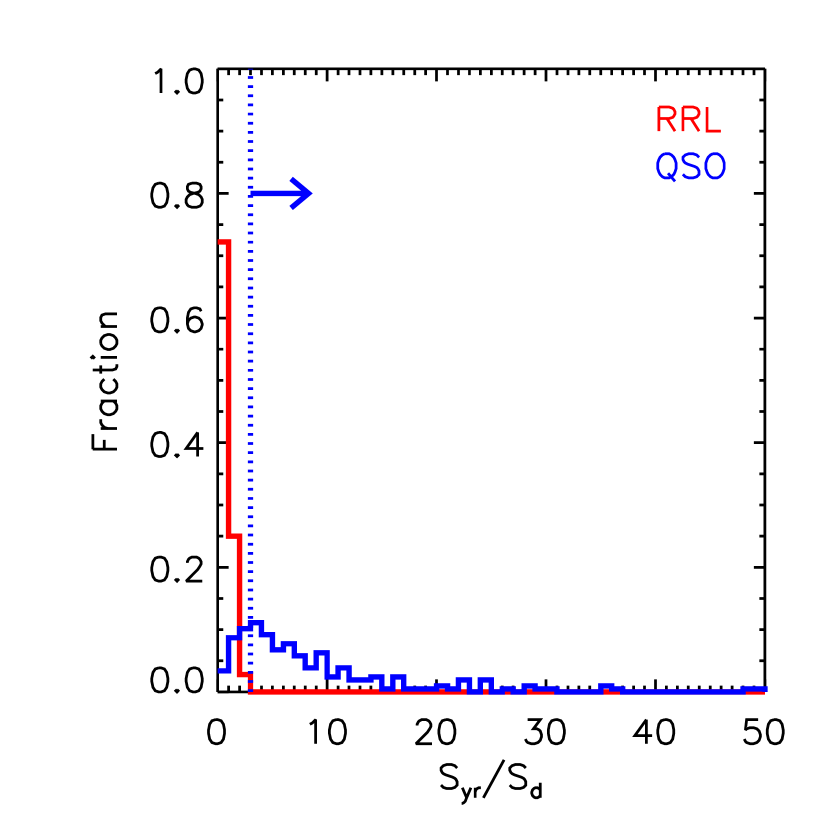
Figure 13.— Histogram of the ratio of the $NUV$ structure function on timescales of years and days for sources classified as RR Lyrae (red) and quasars (blue). Dotted line shows the selection criteria of $S_{\rm y}/S_{\rm d}\geq 3$ used to classify sources with optical point source hosts as quasars.

5.5. X-ray Sources

The archival X-ray catalogs overlap with $\sim 8.45$ deg² of the GALEX TDS survey area. Within this area, 81/89 quasars, 92/105 AGN, and 8/9 M-dwarf stars are detected in the X-rays. In addition, there are 9 optical point sources with X-ray matches that are likely quasars and M dwarfs just outside the quasar and M-dwarf color-color selection regions. UV variability selection appears to be selecting a similar population of active galaxies and M dwarfs as X-ray detection, since $\sim$ 90% of the UV variability-selected active galaxy and M dwarf sample is also detected in the X-rays. However, only 2% of all the X-ray sources (the majority of which are active galaxies) are detected as UV variable at the selection threshold of the GALEX TDS catalog.

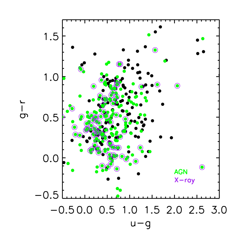
Figure 14.— Colors of archival optical matches to UV variables with extended optical hosts. Sources classified as AGN (by either stochastic UV variability, archival spectra, and/or an X-ray match) are color coded in green. Sources with matches with archival X-ray matches are circled in purple. Note that all galaxy sources with an archival X-ray match are defined as AGNs.

5.6. GUVV Catalog

We also cross-match our GALEX TDS sample with the first and second GALEX Ultraviolet Variability Catalogs (GUVV-1 & GUVV-2) from Welsh et al. (2005) and Wheatley et al. (2008). These catalogs include 894 UV variable sources ($\Delta m>0.6$ mag in the $NUV$) selected from an analysis of archival GALEX AIS, MIS, DIS, and Guest Investigator (GI) fields with repeated observations. With a cross-matching radius of 4 arcsec, we find a match with 36 GUVV sources. For the 15 matches that have GUVV classifications, are all classified by GUVV as active galaxies (AGN or quasars), which are in agreement with our GALEX TDS classifications. Of the 21 matches without GUVV classifications, we find 5 sources classified by GALEX TDS as RR Lyrae, 9 classified as active galaxies (AGN or quasars), 6 with optical point-source hosts, and 1 with a galaxy host.

5.7. Unclassified Sources

The remaining 302 unclassified sources include 91 with optical point-source hosts, which are likely stars, quasars with non-standard colors (high-redshift or reddened), or unresolved galaxies, 190 with galaxy hosts, and 21 orphans. The 190 galaxy hosts may either be faint AGN with poorly constrained UV light curves, or hosts of UV-bright extragalactic transients. In Figure 15 we show the maximum $|\Delta m|$ in the $NUV$ as a function of low-state $NUV$ magnitude of the remaining unclassified sources. The unclassified UV source with the most extreme amplitude, ELAISN1_MOS15-09 with $|\Delta m|>4.2$ mag, was spectroscopically confirmed to be from the nucleus of an inactive galaxy at $z=0.1696$, and its UV/optical flare detected by GALEX TDS and PS1 MDS was attributed to the tidal disruption of a star around a supermassive black hole (Gezari et al., 2012). Also in this sample is a UV transient spectroscopically confirmed to be a Type IIP SN 2010aq at z=0.086 (COSMOS_MOS26-29), whose UV/optical light curve from GALEX TDS and PS1 MDS was fitted with early emission following SN shock breakout in a red supergiant star (Gezari et al., 2010). Both of these spectroscopically classified extragalactic transients are labled in Figure 15.

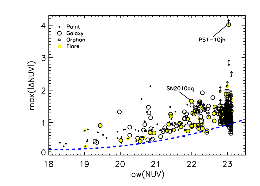
Figure 15.— Maximum $NUV$ variability amplitude for sources without a classification. Dashed blue line shows the median 5$\sigma$ variability selection function as a function of mean magnitude. The nature of the optical host is indicated (point source, galaxy, or orphan), and flaring sources (including transients) are marked in yellow.

Our 5$\sigma$ selection criteria translates to a limiting sensitivity to transients in a host galaxy with a magnitude $m_{\rm host}$ of a magnitude of

$$m_{\rm trans}=-2.5\log(10^{\frac{m_{\rm host}-5\sigma(m_{\rm host})}{-2.5}}-10^{\frac{m_{\rm host}}{-2.5}}),$$ (8)

which ranges from $m_{\rm trans}\sim 20.0$ mag for $m_{\rm host}=18$ mag to $m_{\rm trans}\sim 22.7$ mag for $m_{\rm host}=23$ mag. Thus, our variability selection threshold is less sensitive to transients in host galaxies with bright $NUV$ fluxes. On the red sequence of galaxies, where $M_{\rm NUV}\approx-14.5$ (Wyder et al., 2007), this selection effect is not as much of an issue, since already for $z>0.05$ one gets $m_{\rm host}$ $>$ 22 mag. However, star-forming galaxies on the blue sequence are 2.5 mag brighter in the $NUV$, and thus the host galaxy brightness can be a factor in reducing the senstivity to faint transients. For example, our GALEX TDS 5$\sigma$ sample does not include SN 2009kf, a luminous Type IIP SN in a star-forming galaxy at $z=0.182$ which we reported our GALEX TDS detection of in Botticella et al. (2010). This source varied at only the 4.25$\sigma$ level in the $NUV$ during its peak. However, because this transient was selected from a spatial and temporal coincidence with a PS1 transient alert, we could lower our threshold for variability selection in the UV. The systematic selection of SN and TDE candidates from the joint GALEX TDS and PS1 MDS transient detections will be presented in future papers.

6. Discussion

6.1. Classification Demographics

Figure 16 shows a pie diagram of the source classifications. Out of the total of 1078 GALEX TDS sources, 62% are classified as actively accreting supermassive black holes (quasars or AGN), and 10% as variable and flaring stars (including RR Lyrae, M dwarfs, and CVs). Note that the relative fraction of the different classes of sources is sensitive to both their intrinsic magnitude distribution, and the magnitude-dependent variability selection function of the sample. Table 4 gives the GALEX TDS catalog, sorted by decreasing $NUV$ amplitude, with the GALEX ID, R.A., Dec, low-state $NUV$ magnitude, maximum amplitude of $NUV$ variability ($|\Delta m_{\rm max}|$), intrinsic variability ($\sigma_{int}$), the structure function on day ($S_{\rm d}$) and year ($S_{\rm y}$) timescales, the characteristics of the $NUV$ light curve: flaring (F) or stochastically variable (V), the morphology of the matching optical host: point-source (pt) or extended (ext), the color classification of the matching optical host: RR Lyrae (RRL), M dwarf star (Mdw), star (Star), or quasar (QSO), the archival redshift, an X mark if there is a match with an archival X-ray source, and finally the GALEX TDS classification: RR Lyrae (RRL), M dwarf star (Mdw), star (star), quasar (QSO), AGN, UV flaring source or UV transient source with galaxy host (Galaxy Flare or Galaxy Trans), UV flaring source or transient source with point-source optical host (Point Flare or Point Trans) or UV flaring source or transient source with orphan optical host (Orphan Flare or Orphan Trans), stochastically variable source with a point-source optical host (Point Var), stochastically variable orphan (Orphan Var), or none of the above (?).

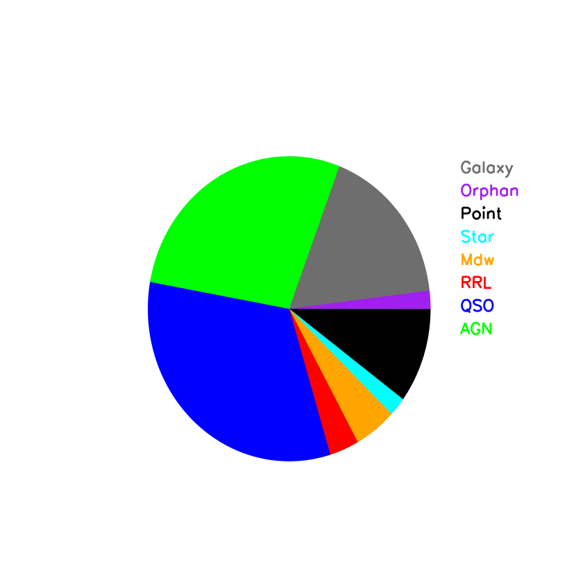
Figure 16.— Pie chart of GALEX TDS classifications: sources classified as stars (Star), M dwarfs (Mdw), RR Lyrae (RRL), quasars (QSO), and active galactic nuclei (AGN), and sources with no classification with galaxy hosts (Galaxy), no host (Orphan), and point-source hosts (Point).

In Figure 17 we show the cummulative surface density distribution of classified UV variable sources as a function of peak magnitude (high(NUV)) and maximum amplitude (max($|\Delta NUV|$)). For the variable UV sources, these correspond to total surface densities of $8.0\pm 3.1$, $7.7\pm 5.8$, and $1.8\pm 1.0$ deg^-2 for quasars, AGNs, and RR Lyrae, respectively. For the transient source, we can calculate a total surface density rate, $\#/(area\times t_{\rm eff})$, where $t_{\rm eff}$ is the effective survey time at the cadence that matches the characteristic timescale of the transient. For extragalactic transients such as young SNe and TDEs, which vary on a timescale of days, we use the time intervals for which the fields were observed with a cadence of $2.0\pm 0.5$ days. If we include all flaring or transient GALEX TDS sources with a galaxy host, this yields a surface density rate of $52\pm 38$ deg^-2 yr^-1 for extragalactic transients. For M dwarfs which vary on timescales shorter than an individual observation, we use the total exposure time for each epoch. If we assume a survey with a cadence of 2 days and $t_{\rm exp}=1.5$ ksec, this translates to a surface density rate for M dwarfs of $15\pm 10$ deg^-2 yr^-1.

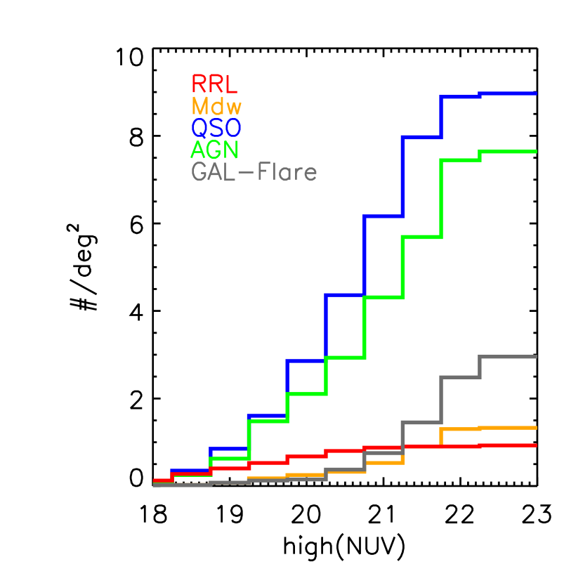
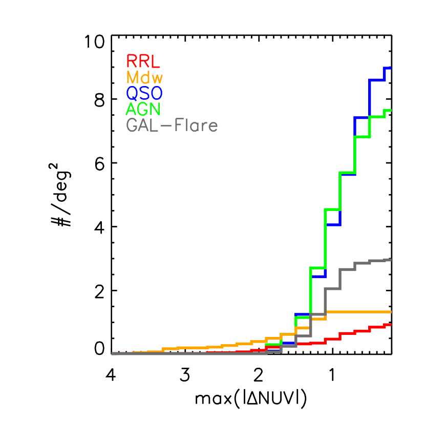
Figure 17.— Cummulative distribution of surface density of UV variable sources with GALEX TDS classifications: M dwarfs (Mdw), RR Lyrae (RRL), quasars (QSO), active galactic nuclei (AGN), and extragalactic transients (GAL-Flare) as a function of peak magnitude (high(NUV)) (left) and maximum amplitude (max($|\Delta NUV|$)) (right).

6.2. UV Variability Properties of Classified Sources

Various optical studies of rest-frame UV variability in high redshift quasars have demonstrated that the variability of AGN increases with decreasing rest wavelength (di Clemente et al., 1996; Vanden Berk et al., 2004; Wilhite et al., 2005). In Figure 18, we show histograms of $\sigma_{int}$ for the UV variable sources with classifications. Quasars show a distribution of $\sigma_{\rm int}$ with a mean that is $\sim 2$ times larger than measured at optical wavelengths from the SDSS Stripe 82 sample from Sesar et al. (2007). This effect is even more pronounced in the magnitude of the structure function on years timescales (S_y), which has a mean that is $5$ times larger than the mean measured in the $r$-band ($\lambda_{eff}=6231)$ from Schmidt et al. (2010). This trend is consistent with the wavelength dependent rise in variability amplitude observed in the structure function for quasars in the rest-frame UV (Vanden Berk et al., 2004) and observed UV (Welsh et al., 2011).

The fact that AGN become bluer during high states of flux (Giveon et al., 1999; Geha et al., 2003; Gezari et al., 2008a) has been attributed to increases in the characteristic temperature of the accretion disk in response to increases in the mass accretion rate (Pereyra et al., 2006; Li & Cao, 2008). However, Schmidt et al. (2012) argue that the color variability observed in individual quasars in their SDSS Stripe 82 sample is stronger than expected from just varying the accretion rate ($\dot{M}$) in accretion disk models. In a future study, we will use simultaneous UV and optical light curves from GALEX TDS and PS1 MDS for our 358 individual quasars to test this result with a larger dynamic range in wavelength.

For the subsample of 95 quasars with archival redshifts ($z_{\rm mean}=1.26$, $\sigma_{z}=0.39$), in Figure 19 we plot $\sigma_{int}$ vs. the low-state $NUV$ absolute magnitude, and find a steep negative correlation fitted by $\log(\sigma_{\rm int})=(1.6\pm 0.1)+\frac{\beta}{2.5}M_{NUV}$, where $\beta=0.24\pm 0.04$, in excellent agreement with the trend for increased variability in lower luminosity quasars seen from optical observations with $\beta=0.246\pm 0.005$ (Vanden Berk et al., 2004), and shallower than expected for a Poissonian process which has $\beta=0.5$ (Cid Fernandes et al., 2000). We also show the subset of 68 AGN with archival redshifts ($z_{\rm mean}=0.64$, $\sigma_{z}=0.55$), which clearly do not show a relation between $\sigma_{\rm int}$ and low-state $NUV$ absolute magnitude. This is most likely a result of dilution of the variability amplitude from the contribution of the host galaxy in the $NUV$.

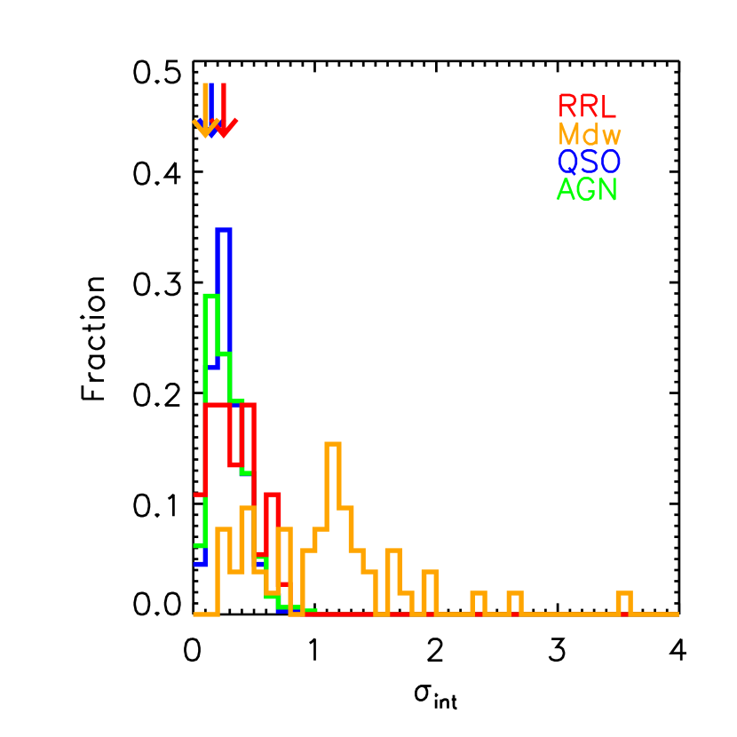
Figure 18.— Intrinsic $NUV$ variability as a function of low-state $NUV$ magnitude for sources classified as RR Lyrae (red), M dwarfs (yellow), quasars (blue) and AGN (green). Arrows shows the median $\sigma_{\rm int}$ measured in the optical for quasars (blue arrow), RR Lyrae (red arrow), and M dwarfs (orange arrow) from Sesar et al. (2007).

The largest values of $|\Delta m|$ (plotted in Figure 10) are found in RR Lyrae and M dwarfs, with a tail of large amplitude variations reaching up to $|\Delta m|=2.9$ mag in RR Lyrae and up to $|\Delta m|=4.6$ mag in M dwarfs. In the optical, the RR Lyrae structure function is very weakly dependent on timescale, with an amplitude of $0.1-0.2$ mag Schmidt et al. (2010). The $NUV$ structure function also shows a weak dependence of amplitude on timescale when comparing the structure function on days to years timescales, however, with an amplitude that is $\sim$3 times larger in the $NUV$ than in the optical. This wavelength dependence on variability amplitude can be explained if the variability is driven by variations in surface temperature from pulsations of the stellar envelope, where higher states of flux are associated with higher temperatures (Sesar et al., 2007).

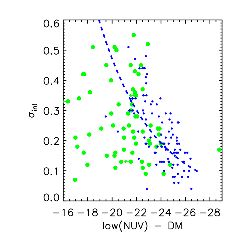
Figure 19.— Intrinsic $NUV$ variability as a function of low-state $NUV$ absolute magnitude, $M_{NUV}$ = low($NUV)-DM$ where $DM$ is the distance modulus, for the subsample of quasars (blue dots) and AGN (green circles) with catalog redshifts. Dashed blue line shows the fit to the quasars to $\log(\sigma_{int})\propto\frac{\beta}{2.5}M$. The spectroscopically classified extragalactic transients (TDE PS1-10jh and SN 2010aq) are labeled.

7. Conclusions

We provide a catalog of over a thousand UV variable sources and their classifications based on optical host properties, UV variability behavior, and cross-matches with archival X-ray and redshift catalogs. This yields a sample of 53 M dwarfs, 37 RR Lyraes, 358 quasars, and 305 AGN. We find median intrinsic UV variability amplitudes in RR Lyrae and quasars that are factors of $>3$ larger than at optical wavelengths, consistent with the expectation for higher temperatures during higher states of flux. The regular cadence and wide area of GALEX TDS enables us to systematically discover persistent and transient (i.e. tidal disruption of a star) accreting supermassive black holes over wide fields of view, study the contemporaneous UV and optical variability of variable stars, and catch young core-collapse supernovae within the first days after explosion. The overlap of the GALEX TDS with PS1 MDS and multiwavelength legacy survey fields will continue to be helpful for classifying transient sources in these heavily observed fields. We also measure the surface densities of variable sources and the surface density rates for transients as a function of class in the UV for the first time.

With GALEX TDS we are only scratching the surface of UV variability. Our 5$\sigma$ sample of 1078 sources is less than 0.3% of the 419,152 UV sources in the field (with an average density of $1.1\times 10^{4}$ UV sources per square degree down to $m_{\rm lim}=23$ mag). Looking to the future, the discovery rate for UV variable sources and UV transients could increase by several orders of magnitude with the launch of a space-based UV mission with a wide field of view (several deg²), a survey strategy of daily cadence observations over $\sim 100$ deg², and detectors with an order of magnitude improved photometric precision relative to GALEX. In the optical sky, 90% of quasars vary with $\sigma_{\rm int}>0.03$ mag on the timescales of years (Sesar et al., 2007). Given the factor of $\sim 2$ larger $\sigma_{\rm int}$ observed for quasars in the $NUV$, one could achieve a nearly complete sample of low-redshift quasars with photometric errors of $\sigma(m)\sim 0.01$ mag. In coordination with a ground-based optical survey, such as Pan-STARRS2 (Burgett, 2012) or LSST , this could yield the simultaneous UV and optical detection of $\approx 10^{4}$ variable quasars and $\approx 10^{3}$ RR Lyrae and M dwarfs, as well as increase the discovery rate of UV-bright extragalactic transients (young SNe and TDEs) by a factor of $\approx 100$.

Table 1GALEX TDS and PS1 MDS

Survey	Field of View	Plate Xcale	PSF FWHM	$m_{\rm lim}$ per Epoch	Cadence	Seasonal Visibility
	(deg)	(arcsec/pixel)	(arcsec)	(mag)	(days)	(months)
GALEX TDS	1.1	1.5	5.3	23.3	2	$\sim 1$
PS1 MDS	3.5	0.258	1.0	23.0	3	$\sim 6$

Table 2GALEX TDS Fields

Name	R.A. (J2000)	Dec (J2000)	$E(B-V)$	Epochs
	(deg)	(deg)	(mag)
PS_XMMLSS_MOS00	35.580	$-$3.140	0.028	27
PS_XMMLSS_MOS01	36.500	$-$3.490	0.025	27
PS_XMMLSS_MOS02	35.000	$-$3.950	0.020	14
PS_XMMLSS_MOS03	35.875	$-$4.250	0.026	27
PS_XMMLSS_MOS04	36.900	$-$4.420	0.026	27
PS_XMMLSS_MOS05	35.200	$-$5.050	0.022	26
PS_XMMLSS_MOS06	36.230	$-$5.200	0.027	24
PS_CDFS_MOS00	53.100	$-$27.800	0.008	114
PS_CDFS_MOS01	52.012	$-$28.212	0.008	30
PS_CDFS_MOS02	53.124	$-$26.802	0.009	29
PS_CDFS_MOS03	54.165	$-$27.312	0.012	30
PS_CDFS_MOS04	52.910	$-$28.800	0.009	30
PS_CDFS_MOS05	52.111	$-$27.276	0.010	30
PS_CDFS_MOS06	53.970	$-$28.334	0.010	6
PS_COSMOS_MOS21	150.500	$+$3.100	0.023	15
PS_COSMOS_MOS22	149.500	$+$3.100	0.027	16
PS_COSMOS_MOS23	151.000	$+$2.200	0.024	24
PS_COSMOS_MOS24	150.000	$+$2.200	0.020	26
PS_COSMOS_MOS25	149.000	$+$2.300	0.023	13
PS_COSMOS_MOS26	150.500	$+$1.300	0.023	26
PS_COSMOS_MOS27	149.500	$+$1.300	0.019	27
PS_GROTH_MOS01	215.600	$+$54.270	0.011	17
PS_GROTH_MOS02	213.780	$+$54.350	0.015	16
PS_GROTH_MOS03	214.146	$+$53.417	0.009	17
PS_GROTH_MOS04	212.400	$+$53.700	0.011	18
PS_GROTH_MOS05	215.500	$+$52.770	0.008	19
PS_GROTH_MOS06	214.300	$+$52.550	0.008	8
PS_GROTH_MOS07	212.630	$+$52.750	0.009	19
PS_ELAISN1_MOS10	242.510	$+$55.980	0.007	17
PS_ELAISN1_MOS11	244.570	$+$55.180	0.009	17
PS_ELAISN1_MOS12	242.900	$+$55.000	0.008	18
PS_ELAISN1_MOS13	241.300	$+$55.350	0.007	18
PS_ELAISN1_MOS14	243.960	$+$54.200	0.010	19
PS_ELAISN1_MOS15	242.400	$+$54.000	0.011	21
PS_ELAISN1_MOS16	241.380	$+$54.450	0.010	19
PS_VVDS22H_MOS00	333.700	$+$1.250	0.040	39
PS_VVDS22H_MOS01	332.700	$+$0.700	0.046	35
PS_VVDS22H_MOS02	334.428	$+$0.670	0.057	38
PS_VVDS22H_MOS03	333.600	$+$0.200	0.058	27
PS_VVDS22H_MOS04	334.610	$-$0.040	0.093	24
PS_VVDS22H_MOS05	333.900	$-$0.720	0.102	35
PS_VVDS22H_MOS06	332.900	$-$0.400	0.113	33

Table 3GALEX TDS Classifications

		Archive		PS1		Classification
Step	$N_{\rm unclass}$	pt	ext	pt	ext	orphan	QSO	RRL	Mdw	Star	AGN	pt	gal
optical match	1078	487	391	76	103	21
QSO color cut	1078	326					326
RRL color cut	753	37						37
Mdw color cut	716	44		9					53
stellar locus color cut	663	17								17
$S_{\rm yr}/S_{\rm d}\geq 3$	646	19		15			34
stochastic UV var	616		200		68						268
X-ray/spec match	346	8	37				2			5	37
	302					21	358	37	53	22	305	93	189

Table 4GALEX TDS Catalog

	NUV								Optical				X-ray	Class
ID	R.A.	Dec	mlow	$|\Delta m_{\rm max}|$	$\sigma_{int}$	Sd	Syr	LC	Morph	$r_{\rm AB}$	Color	$z$
GROTH_MOS01-21	216.1622	54.0911	22.54	4.60	1.04	0.80	1.13	V	pt	14.92	Mdw			Mdw
VVDS22H_MOS05-05	333.8326	-0.5491	21.14	4.47	0.99	0.90	0.74	F	pt	21.24	QSO			CV
ELAISN1_MOS15-02	242.0397	54.3586	$>$22.89	$>$4.03	1.37	0.84	2.93	V	pt	22.51	QSO			CV
ELAISN1_MOS15-09	242.3685	53.6738	$>$23.03	$>$4.02	1.23	0.01	2.15	F	ext	21.05				Galaxy Trans
GROTH_MOS07-09	212.5024	52.4153	$>$23.10	$>$3.61	3.51	0.09	0.69	F	pt	17.45	Mdw			Mdw
CDFS_MOS02-20	53.1682	-26.3564	$>$23.06	$>$3.60	0.73	0.95	0.78		$\cdots$	15.72	Mdw			Mdw
CDFS_MOS00-41	53.3453	-27.3361	$>$23.10	$>$3.36	0.36	0.39	0.15	V	$\cdots$	15.76				Mdw
COSMOS_MOS22-11	149.4973	3.1171	22.56	3.35	0.75	$\cdots$	0.58	F	pt	14.25	Mdw			Mdw
GROTH_MOS05-00	214.9435	52.9953	22.07	3.29	0.71	1.18	0.65	F	pt	14.15	Mdw		X	Mdw
XMMLSS_MOS06-22	36.6468	-5.0886	$>$22.95	$>$3.28	0.95	$<$0	4.04		pt	15.58	Mdw		X	Mdw

References

- Aihara et al. (2011) Aihara, H., et al. 2011, ApJS, 193, 29
- Bianchi et al. (2011) Bianchi, L., Efremova, B., Herald, J., Girardi, L., Zabot, A., Marigo, P., & Martin, C. 2011, MNRAS, 411, 2770
- Botticella et al. (2010) Botticella, M. T., et al. 2010, ArXiv e-prints, 1001.5427
- Brown et al. (2009) Brown, P. J., et al. 2009, AJ, 137, 4517
- Budavári & Szalay (2008) Budavári, T., & Szalay, A. S. 2008, ApJ, 679, 301
- Burgett (2012) Burgett, W. S. 2012, ArXiv e-prints, 1207.3460
- Chevalier & Irwin (2011) Chevalier, R. A., & Irwin, C. M. 2011, ApJ, 729, L6
- Chiappetti et al. (2005) Chiappetti, L., et al. 2005, A&A, 439, 413
- Cid Fernandes et al. (2000) Cid Fernandes, R., Sodré, Jr., L., & Vieira da Silva, Jr., L. 2000, ApJ, 544, 123
- Civano et al. (2012) Civano, F., et al. 2012, ArXiv e-prints, 1205.5030
- di Clemente et al. (1996) di Clemente, A., Giallongo, E., Natali, G., Trevese, D., & Vagnetti, F. 1996, ApJ, 463, 466
- Elvis et al. (2009) Elvis, M., et al. 2009, ApJS, 184, 158
- Geha et al. (2003) Geha, M., et al. 2003, AJ, 125, 1
- Gezari et al. (2008a) Gezari, S., et al. 2008a, ApJ, 676, 944
- Gezari et al. (2012) ——. 2012, Nature, 485, 217
- Gezari et al. (2008b) ——. 2008b, ApJ, 683, L131
- Gezari et al. (2009) ——. 2009, ApJ, 698, 1367
- Gezari et al. (2006) ——. 2006, ApJ, 653, L25
- Gezari et al. (2010) ——. 2010, ApJ, 720, L77
- Giacconi et al. (2002) Giacconi, R., et al. 2002, ApJS, 139, 369
- Giveon et al. (1999) Giveon, U., Maoz, D., Kaspi, S., Netzer, H., & Smith, P. S. 1999, MNRAS, 306, 637
- Hasinger et al. (2007) Hasinger, G., et al. 2007, ApJS, 172, 29
- Hook et al. (1994) Hook, I. M., McMahon, R. G., Boyle, B. J., & Irwin, M. J. 1994, MNRAS, 268, 305
- Huber et al. (2011) Huber, M., et al. 2011, in American Astronomical Society Meeting Abstracts 218, 328.12
- Kaiser et al. (2010) Kaiser, N., et al. 2010, in Society of Photo-Optical Instrumentation Engineers (SPIE) Conference Series, Vol. 7733, Society of Photo-Optical Instrumentation Engineers (SPIE) Conference Series
- Kowalski et al. (2009) Kowalski, A. F., Hawley, S. L., Hilton, E. J., Becker, A. C., West, A. A., Bochanski, J. J., & Sesar, B. 2009, AJ, 138, 633
- Laird et al. (2009) Laird, E. S., et al. 2009, ApJS, 180, 102
- Le Fèvre et al. (2005) Le Fèvre, O., et al. 2005, A&A, 439, 845
- Le Fèvre et al. (2004) ——. 2004, A&A, 428, 1043
- Lehmer et al. (2005) Lehmer, B. D., et al. 2005, ApJS, 161, 21
- Li & Cao (2008) Li, S.-L., & Cao, X. 2008, MNRAS, 387, L41
- Lilly et al. (2009) Lilly, S. J., et al. 2009, ApJS, 184, 218
- Lilly et al. (2007) ——. 2007, ApJS, 172, 70
- Magnier (2006) Magnier, E. 2006, in The Advanced Maui Optical and Space Surveillance Technologies Conference
- Manners et al. (2003) Manners, J. C., et al. 2003, MNRAS, 343, 293
- Martin et al. (2005) Martin, D. C., et al. 2005, ApJ, 619, L1
- Milne et al. (2010) Milne, P. A., et al. 2010, ApJ, 721, 1627
- Morrissey et al. (2007) Morrissey, P., et al. 2007, ApJS, 173, 682
- Nakar & Sari (2010) Nakar, E., & Sari, R. 2010, ApJ, 725, 904
- Nandra et al. (2005) Nandra, K., et al. 2005, MNRAS, 356, 568
- Newman et al. (2012) Newman, J. A., et al. 2012, ArXiv e-prints, 1203.3192
- Ofek et al. (2010) Ofek, E. O., et al. 2010, ApJ, 724, 1396
- Pereyra et al. (2006) Pereyra, N. A., Vanden Berk, D. E., Turnshek, D. A., Hillier, D. J., Wilhite, B. C., Kron, R. G., Schneider, D. P., & Brinkmann, J. 2006, ApJ, 642, 87
- Pierre et al. (2007) Pierre, M., et al. 2007, MNRAS, 382, 279
- Rabinak & Waxman (2011) Rabinak, I., & Waxman, E. 2011, ApJ, 728, 63
- Regnault et al. (2009) Regnault, N., et al. 2009, A&A, 506, 999
- Rest et al. (2005) Rest, A., et al. 2005, ApJ, 634, 1103
- Richards et al. (2002) Richards, G. T., et al. 2002, AJ, 123, 2945
- Schawinski et al. (2008) Schawinski, K., et al. 2008, Science, 321, 223
- Schlafly et al. (2012) Schlafly, E. F., et al. 2012, ApJ, 756, 158
- Schlegel et al. (1998) Schlegel, D. J., Finkbeiner, D. P., & Davis, M. 1998, ApJ, 500, 525
- Schmidt et al. (2010) Schmidt, K. B., Marshall, P. J., Rix, H.-W., Jester, S., Hennawi, J. F., & Dobler, G. 2010, ApJ, 714, 1194
- Schmidt et al. (2012) Schmidt, K. B., Rix, H.-W., Shields, J. C., Knecht, M., Hogg, D. W., Maoz, D., & Bovy, J. 2012, ApJ, 744, 147
- Sesar et al. (2010) Sesar, B., et al. 2010, ApJ, 708, 717
- Sesar et al. (2007) ——. 2007, AJ, 134, 2236
- Stubbs et al. (2010) Stubbs, C. W., Doherty, P., Cramer, C., Narayan, G., Brown, Y. J., Lykke, K. R., Woodward, J. T., & Tonry, J. L. 2010, ApJS, 191, 376
- Surace et al. (2004) Surace, J. A., et al. 2004, VizieR Online Data Catalog, 2255, 0
- Svirski et al. (2012) Svirski, G., Nakar, E., & Sari, R. 2012, ApJ, 759, 108
- Szkody et al. (2011) Szkody, P., et al. 2011, AJ, 142, 181
- Tonry et al. (2012) Tonry, J. L., et al. 2012, ApJ, 750, 99
- Trammell et al. (2007) Trammell, G. B., Vanden Berk, D. E., Schneider, D. P., Richards, G. T., Hall, P. B., Anderson, S. F., & Brinkmann, J. 2007, AJ, 133, 1780
- Trump et al. (2009) Trump, J. R., et al. 2009, ApJ, 696, 1195
- Trump et al. (2007) ——. 2007, ApJS, 172, 383
- Vanden Berk et al. (2004) Vanden Berk, D. E., et al. 2004, ApJ, 601, 692
- Virani et al. (2006) Virani, S. N., Treister, E., Urry, C. M., & Gawiser, E. 2006, AJ, 131, 2373
- Voges et al. (1999) Voges, W., et al. 1999, VizieR Online Data Catalog, 9010, 0
- Voges et al. (2000) ——. 2000, VizieR Online Data Catalog, 9029, 0
- Welsh et al. (2005) Welsh, B. Y., et al. 2005, AJ, 130, 825
- Welsh et al. (2011) Welsh, B. Y., Wheatley, J. M., & Neil, J. D. 2011, A&A, 527, A15
- Welsh et al. (2007) Welsh, B. Y., et al. 2007, ApJS, 173, 673
- West et al. (2011) West, A. A., et al. 2011, AJ, 141, 97
- Wheatley et al. (2012) Wheatley, J., Welsh, B. Y., & Browne, S. E. 2012, PASP, 124, 552
- Wheatley et al. (2008) Wheatley, J. M., Welsh, B. Y., & Browne, S. E. 2008, AJ, 136, 259
- Wilhite et al. (2005) Wilhite, B. C., Vanden Berk, D. E., Kron, R. G., Schneider, D. P., Pereyra, N., Brunner, R. J., Richards, G. T., & Brinkmann, J. V. 2005, ApJ, 633, 638
- Wyder et al. (2007) Wyder, T. K., et al. 2007, ApJS, 173, 293
- Yanny et al. (2009) Yanny, B., et al. 2009, AJ, 137, 4377