Time-evolution of tripartite quantum discord and entanglement under local and non-local random telegraph noise

Abstract

Few studies explored the dynamics of non-classical correlations besides entanglement in open multipartite quantum systems. Here, we address the time-evolution of quantum discord and entanglement in a model of three non-interacting qubits subject to a classical random telegraph noise in common and separated environments. Two initial entangled states of the system are examined, namely the GHZ- and W-type states. The dynamics of quantum correlations results to be strongly affected by the input configuration of the qubits, the type of the system-environment interaction, and the memory properties of the environmental noise. When the qubits are non-locally coupled to the random telegraph noise, the GHZ-type states partially preserve, at long times, both discord and entanglement, regardless the correlation time of the environmental noise. The survived entangled states turn out to be also detectable by means of suitable entanglement witnesses. On the other hand, in the same conditions, the decohering effects suppress all the quantum correlation of the W-type states which are thus less robust than the GHZ-type ones. The long-time survival of tripartite discord and entanglement opens interesting perspectives in the use of multipartite entangled states for practical applications in quantum information science.

.

I Introduction

Entanglement is a peculiar feature of quantum mechanics which constitutes a valuable resource for a number of features of quantum information processing, such as quantum communication, cryptography, and computation Nielsen and Chuang (2000). However, the major limitation of the use of entanglement in practical applications is due to the unavoidable interaction of the real quantum systems with their surroundings, resulting in decoherence processes, and, as a consequence, in degradation of the entangled states Joos et al. (2003). Therefore, many research efforts focused on the investigation of the decoherence processes and of the dynamics of entanglement in different quantum systems ranging from quantum optics Yu and Eberly (2004); Bellomo et al. (2008); Maniscalco et al. (2008); An et al. (2011) to nanophysics (Buscemi et al., 2009; *Buscemi2010; *Buscemi2011). The decohering effects of the environments with different memory properties have widely been studied in bipartite systems where entanglement can exhibit peculiar features including sudden death and transitions, revivals, and trapping Yu and Eberly (2004); Bellomo et al. (2007, 2008); Maniscalco et al. (2008). On the other hand, only recently the time evolution of the entanglement has begun to be analyzed in multipartite open quantum systems, since in such systems the characterization and quantification of the quantum correlations still represent a hard task. Specifically, different approaches have been used Casagrande et al. (2009); Altintas and Eryigit (2010); Man et al. (2010); Anza et al. (2010); An et al. (2011); Siomau and Fritzsche (2010); Siomau (2012); Ma et al. (2010); Ann and Jaeger (2008); Liu et al. (2010); Weinstein (2009, 2010). Some of them involve the generalization of entanglement measures ranging from negativity (Casagrande et al., 2009; *Altintas; *Zhong-Xiao; *Anza) to concurrence An et al. (2011); Siomau and Fritzsche (2010); *Siomau2 or Bell nonlocality disequalities (Ma et al., 2010; *Ann; *Liu) commonly adopted in bipartite systems. Multipartite entanglement has also been investigated by means of suitable entanglement witnesses (EWs), namely observables that can detect the presence of the entanglement itself Acin et al. (2000); Weinstein (2009, 2010).

Apart from entanglement, quantum states can exhibit other correlations not present in classical systems. In particular, in the last years quantum discord (QD) has received an increasing attention as a mean to estimate the quantum correlations encoded in a system and potentially usable for applications in quantum informations processing Ollivier and Zurek (2001); Henderson and Vedral (2001); Werlang et al. (2009a); Mazzola et al. (2010); Fanchini et al. (2010). Indeed, it was shown theoretically Datta et al. (2008), and later experimentally Lanyon et al. (2008), that bipartite separable mixed states with nonzero discord may provide computational speedup compared to classical states in some quantum computation protocols. Under suitable conditions quantum discord is also found to be more robust than entanglement in noisy environments Werlang et al. (2009a). While the characterization of quantum discord in terms of the discrepancy between two quantum analogues of the classical mutual information has well been grasped and widely used in bipartite systems, its extensions in multipartite systems is still discussed and tackled with different approaches Kaszlikowski et al. (2008); Rulli and Sarandy (2011); Chakrabarty et al. (2011); Grimsmo et al. (2012); Giorgi et al. (2011); Zhao et al. (2012). Recently, Giorgi et al. Giorgi et al. (2011) introduced a measure of genuine total, classical, and quantum correlations relying on the use of relative entropy to quantify the distance between two density matrices. Like other proposed measures of correlations in quantum systems Rulli and Sarandy (2011); Chakrabarty et al. (2011); Zhao et al. (2012), the approach of Ref. Giorgi et al. (2011) involves difficult extremization procedures over operators or states which makes the calculations very hard. This justifies the scarse number of works exploring the time evolution of quantum correlations in multipartite open systems.

In this paper, we investigate the dynamics of the quantum correlations in a physical model consisting of three qubits, not interacting among each other, and subject to a classical random telegraph noise (RTN). Two different initial configurations are examined, namely GHZ and W Werner type-states. The influence of the classical environmental noise on the system is described by means of a stochastic Hamiltonian with a coupling term mimicking a random telegraph signal. The dynamics of the two qubits is evaluated by averaging the time-evolved states over the noise. Even if in similar systems of two qubits the time evolution of quantum correlations has already been investigated Zhou et al. (2010); De et al. (2011); Möttönen et al. (2006); Bordone et al. (2012); *BenedettiAr, the analysis of the tripartite regime seems quite promising since here the correlations derive from a more complex scenario, and, as a consequence, more peculiar phenomena are expected.

The use of a stochastic Hamiltonian allows us to evaluate the dynamics of qubits in both separated common environments in a straightforward way. While in the former case each subsystem is locally coupled to a source of RTN, in the latter a non-local interaction between the entire system and the environment occurs, being the qubits collectively coupled to the same source of RTN. This gives us the chance to analyze how the local or non-local nature of the qubits-environment coupling and the memory properties of the environment itself affect the dynamics of quantum correlation and its possible sudden death, revival, or trapping. From this point of view, the choice of a classical environment does not represent a strict constraint of the model, since a quantum environment not affected by the system or influenced in a way that does not result in back-action, can be mimicked by a classical noise Saira et al. (2007) that was already shown to be able to lead, in bipartite systems, to sudden death and revival of entanglement and discord Zhou et al. (2010); Benedetti et al. (2012); Lo Franco et al. (2012).

Here, we focus on the quantum correlations in the form of tripartite entanglement and quantum discord. Being the characterization of tripartite mixed entangled states still debated, two different estimators are adopted to evaluate analytically the entanglement in agreement with what was done in other works Weinstein (2009, 2010). One estimator is the tripartite negativity Sabin and Garcia-Alcaine (2008), which was shown to play a key role in quantum information protocols since states exhibiting nonzero tripartite negativity are distillable to GHZ states. The other estimator relies on the concept of detectable entanglement and uses suitable EWs Acin et al. (2000). The quantum discord is numerically quantified by using the approach developed in Ref. Giorgi et al. (2011). Unlike the tripartite negativity and the expectation value of the EWs, in this case we need to use numerical techniques apt to optimize, over positive operator-valued measures (POVM’s) and subsystems, the conditional entropies appearing in the definition of discord. The comparison between the time evolution of these estimators for two different initial configurations of the qubits can represent a valid guideline to shed some light on the discrepancies and the analogies between the two forms of correlation in our model.

The paper is organized as follows: in Sec. II, we introduce the estimators used to quantify tripartite quantum discord, entanglement, and detectable entanglement. In Sec. III, we illustrate the physical model consisting of three qubits subject to a classical RTN within common or different environments. Sec. IV reports the time evolution of quantum correlations for two initial configurations of the qubits in the case of local and non-local system-environment interaction. Finally, conclusions and discussions are summarized in Sec. V.

II Quantum correlation measures in tripartite systems

In this section, we briefly expose the correlations measures adopted in our work to quantify and characterize the tripartite quantum discord and entanglement.

II.1 Tripartite Quantum Discord

Here, we illustrate the criterion adopted to quantify the genuine total, classical, and quantum correlations in a tripartite system. By following the approach used in Ref. Giorgi et al. (2011), the genuine total correlations $\mathcal{T}^{(3)}(\rho)$, of a mixed state $\rho$ can be expressed as:

$$\mathcal{T}^{(3)}(\rho)=\mathcal{T}(\rho)-\mathcal{T}^{(2)}(\rho),$$ (1)

where $\mathcal{T}(\rho)$ is the quantum extension of the Shannon classical mutual information

$$\mathcal{T}(\rho)=S(\rho_{A})+S(\rho_{B})+S(\rho_{C})-S(\rho)$$ (2)

with $S(\rho_{K})$=$-\textrm{Tr}\big{(}\rho_{K}\ln_{2}{\rho_{K}}\big{)}$ indicating the the von Neumann entropy of $\rho_{K}$. $\mathcal{T}^{(2)}(\rho)$ is given by the maximum of the total bipartite correlations among two qubits of the system, namely

$$\mathcal{T}^{(2)}(\rho)=\max{\left[\mathcal{I}^{(2)}(\rho_{A,B}),\mathcal{I}^{(2)}(\rho_{A,C}),\mathcal{I}^{(2)}(\rho_{B,C})\right]}$$ (3)

with $\mathcal{I}^{(2)}(\rho_{I,J})$=$S(\rho_{I})+S(\rho_{J})-S(\rho_{IJ})$ denoting the bipartite quantum mutual information of the subsystem consisting of the two qubits $I$ and $J$. By inserting Eqs. (2) and (3) in (1), one finds

$$\mathcal{T}^{(3)}(\rho)=$$ (4)

$$\min{\left[\mathcal{I}^{(2)}(\rho_{A,BC}),\mathcal{I}^{(2)}(\rho_{B,AC}),\mathcal{I}^{(2)}(\rho_{C,AB})\right]},$$

that is the total correlations of the state $\rho$ are the lowest bipartite mutual information between the one-qubit part and the two-qubit part. As indicated in Ref. Giorgi et al. (2011), $\mathcal{T}^{(3)}(\rho)$ estimates the amount of genuine tripartite correlations that cannot be accounted for considering any of the possible subsystems.

Analogously with $T^{(3)}(\rho)$ , also the genuine classical correlations $\mathcal{J}^{(3)}(\rho)$ can be defined in terms of the difference between the total classical ones $\mathcal{J}(\rho)$ and the maximum among bipartite correlations $\mathcal{J}^{(2)}(\rho)$:

$$\mathcal{J}^{(3)}(\rho)=\mathcal{J}(\rho)-\mathcal{J}^{(2)}(\rho).$$ (5)

Here

$$\mathcal{J}(\rho)=$$ (6)

$$\max_{I,J,K}{\left[S(\rho_{I})-S(\rho_{I|J})+S(\rho_{K})-S(\rho_{K|IJ})\right]},$$

denotes the maximum over the six possible quantum extensions of the conditional entropy which, in turn, is maximized on the complete measurement on two subparties where

$$S(\rho_{I|J})=\min_{\{E^{m}_{J}\}}\sum_{m}p_{m}S(\rho_{I|E_{m}^{J}})\quad\textrm{with}\quad p_{m}=\textrm{Tr}_{IJ}\left(E_{m}^{J}\rho_{IJ}\right),\rho_{I|E_{m}^{J}}=\frac{\textrm{Tr}_{J}E_{m}^{J}\rho_{IJ}}{p_{m}}$$ (7)

$$S(\rho_{K|IJ})=\min_{\{E^{I}_{l},E^{J}_{m}\}}\sum_{l,m}p_{lm}S(\rho_{K|E_{m}^{J}E_{l}^{I}})\quad\textrm{with}\quad p_{lm}=\textrm{Tr}_{IJK}\left(E_{l}^{I}E_{m}^{J}\rho\right),\rho_{K|E_{m}^{J}E_{l}^{I}}=\frac{\textrm{Tr}_{IJ}E_{l}^{I}E_{m}^{J}\rho}{p_{lm}}.$$

In the above expressions, $\{E^{I}_{l}\}$, and $\{E^{J}_{m}\}$ indicate the POVM’s acting on the qubits $I$ and $J$, respectively. On the other hand, $\mathcal{J}^{(2)}(\rho)$ corresponds to the maximum of the classical bipartite correlations among two qubits of the system

$$\mathcal{J}^{(2)}(\rho)=$$ (8)

$$\max{\left[\mathcal{J}^{(2)}(\rho_{A,B}),\mathcal{J}^{(2)}(\rho_{A,C}),\mathcal{J}^{(2)}(\rho_{B,C})\right]},$$

where $\mathcal{J}^{(2)}(\rho_{I,J})$=$\max\left[\mathcal{J}^{(2)}_{I:J}(\rho_{I,J}),\mathcal{J}^{(2)}_{J:I}(\rho_{I,J})\right]$ with $\mathcal{J}^{(2)}_{I:J}(\rho_{I,J})$=$S(\rho_{I})-S(\rho_{I|J})$.

In agreement with the usual definition for two-qubit systems Ollivier and Zurek (2001); Henderson and Vedral (2001), the tripartite quantum discord $\mathcal{D}^{(3)}(\rho)$ can be expressed as

$$\mathcal{D}^{(3)}(\rho)=\mathcal{T}^{(3)}(\rho)-\mathcal{J}^{(3)}(\rho).$$ (9)

Given the optimization procedures over the indices and POVMs appearing in the formal expression of $\mathcal{T}^{(3)}(\rho)$ and $\mathcal{J}^{(3)}(\rho)$, the evaluation of Eq. (9) is not immediate. For symmetrical states, namely those systems whose state is invariant under the permutations of the three parties, it can be shown that the tripartite total, classical, and quantum correlations can be evaluated by means of simple expressions. After a straightforward calculation, one finds

$$\mathcal{T}^{(3)}(\rho) = S(\rho_{C})+S(\rho_{AB})-S(\rho)$$

$$\mathcal{J}^{(3)}(\rho) = S(\rho_{C})-S(\rho_{C|AB})$$

$$\mathcal{D}^{(3)}(\rho) = S(\rho_{AB})+S(\rho_{C|AB})-S(\rho).$$ (10)

These are formally equivalent to the forms reported in Ref. Zhao et al. (2012) but here, in agreement with the approach developed by Giorgi et al. Giorgi et al. (2011) the von Neumann entropy of the measurement-based conditional density operator $\rho_{C|AB}$ is minimized over the set of two-qubit POVM’s factorizable in terms of single-qubit POVM’s $E_{m}^{A}\otimes E_{n}^{B}$. The use of the latter as optimal POVM in the definition of classical tripartite correlations has been discussed Zhao et al. (2012). In our numerical approach the von Neumann entropy of the measurement-based conditional density operator given in Eqs. (7) has been estimated by using projective measurements described by the complete set of orthogonal projectors $\Pi^{AB}_{mn}(\theta_{A},\theta_{B},\Phi_{A},\Phi_{B})$=$\sum_{m,n}|\widetilde{m}_{A}\widetilde{n}_{B}\rangle\langle\widetilde{n}_{B}\widetilde{m}_{A}|$ (with $m,n=0,1$) defined by the orthogonal states

$$|\widetilde{0}_{A(B)}\rangle = \cos{\theta_{A(B)}}|0\rangle+e^{i\Phi_{A(B)}}\sin{\theta_{A(B)}}|1\rangle$$

$$|\widetilde{1}_{A(B)}\rangle = e^{-i\Phi_{A(B)}}\sin{\theta_{A(B)}}|0\rangle-\cos{\theta_{A(B)}}|1\rangle.$$ (11)

The conditional entropy $S(\rho_{C|AB})$ has been minimized over the phases $\theta_{A}$, $\theta_{B}$, $\Phi_{A}$, and $\Phi_{B}$.

In the followings, we will use Eqs. (II.1) to evaluate the dynamics of quantum discord since at any time $t$ the system investigated is invariant under the permutations of the three qubits.

II.2 Tripartite Negativity

In order to quantify the three-qubit entanglement of a mixed state $\rho$, we use the tripartite negativity $\mathcal{N}^{(3)}$ which is given by Sabin and Garcia-Alcaine (2008):

$$\mathcal{N}^{(3)}(\rho)=\sqrt[3]{\mathcal{N}_{A-BC}\mathcal{N}_{B-AC}\mathcal{N}_{C-AB}}.$$ (12)

It is the geometric mean of the bipartite negativities $\mathcal{N}_{I-JK}$ (where $I$=$A,B,C$ and $JK$=$BC,AC,AB$), which, in turn, are defined as $\mathcal{N}_{I-JK}$=$\sum_{i}\left|a_{i}(\rho^{T_{I}})\right|-1$, with $a_{i}(\rho^{T_{I}})$ the eigenvalues of the partial transpose $\rho^{T_{I}}$ of the total density matrix with respect to the subsystem $I$. For symmetrical tripartite quantum systems, $\mathcal{N}^{(3)}$ reduces to the bipartite negativity of any bipartition of the system. Recently, $\mathcal{N}^{(3)}$ has also been used to estimate the entanglement of tripartite bosonic and fermionic systems Buscemi and Bordone (2011).

Even if the positivity of the tripartite negativity ensures that the state of the system under investigation is not separable and distillable to a GHZ state, $\mathcal{N}^{(3)}$ cannot be used to classify and fully characterize the entanglement of general mixed tripartite states Sabin and Garcia-Alcaine (2008) Apart from pure states, null tripartite negativity could indeed not imply the absence of entanglement.

II.3 Entanglement Witnesses

Multipartite entanglement can also be investigated by means of entanglement witnesses (EWs), namely suitable observables that, at least in principle, can be experimentally implemented to detect the presence of entanglement Acin et al. (2000); Weinstein (2009, 2010). Following the classification of Ref. Acin et al. (2000), four classes of three-qubit mixed states can be defined: separable states (S), biseparable states (B), W states, and GHZ states. Note that each class includes within it the previous classes as special cases. EWs are suitable observables whose expectation value is zero or positive for all the states belonging to a specific class and negative for at least one state of higher class, namely a more inclusive class. Thus the use of EWs allows one to determine which class a given state belongs.

Specifically, in this work we will use those EWs that permit to identify whether a state is in the $W$-$B$ class, namely a state with true tripartite entanglement either of the GHZ-type or W-type and not biseparable. As shown in Refs. Acin et al. (2000); Weinstein (2009), GZH-type states in the $W$-$B$ class can be detected by means of

$$\mathcal{W}_{W2}=\frac{1}{2}I-P_{GHZ},$$ (13)

where $P_{GHZ}$ is the projector onto $|GHZ\rangle$. On the other hand, for W-type states, we will use the EW

$$\mathcal{W}_{W1}=\frac{2}{3}I-P_{W}.$$ (14)

with $P_{W}$ the projector onto $|W\rangle$. Negative expectation values of the observables of the Eqs. (13) and (14) indicate the appearance of tripartite entanglement experimentally detectable in the system. However, zero or positive values do not guarantee the absence of entanglement.

III The model

Here, we describe a model consisting of three non-interacting qubits subject to an environmental classical RTN. The system-environment coupling is here analyzed in two different conditions. In the first one, each qubit locally interacts with its environment. In the other case, all the qubits are coupled with a unique common source of RTN thus mimicking a non-local interaction between the qubits themselves and environment. In both configurations, the dynamics of the system is ruled by the Hamiltonian

$$\mathcal{H}(t)=\mathcal{H}_{A}(t)\otimes I_{BC}+\mathcal{H}_{B}(t)\otimes I_{AC}+\mathcal{H}_{C}(t)\otimes I_{AB},$$ (15)

where $I_{JK}$ is the identity operator in the subspace of the two qubits $J$ and $K$ and $\mathcal{H}_{L}(t)$ denotes the single-qubit Hamiltonian Bordone et al. (2012); Benedetti et al. (2012)

$$\mathcal{H}_{L}(t)=\varepsilon I_{L}+\nu\eta_{L}(t){\sigma_{x}}_{L},$$ (16)

with ${\sigma_{x}}_{L}$ indicating the Pauli matrix of the subspace of the qubit $L$. $\varepsilon$ is the qubit energy in the absence of noise (energy degeneracy is assumed), $\nu$ is the system-environment coupling constant. The RTN is here introduced by means the stochastic process denoted by $\eta_{L}(t)$ describing a fluctuator randomly flipping between the values -1 and 1 at rate $\gamma$. The two-particle form of the model defined by Eqs. (15) and (16) has already been used to evaluate the time behavior of entanglement and quantum discord (Bordone et al., 2012; *BenedettiAr). Furthermore its extension to qudits case allows also to analyze the quantum walks of not-interacting particles in one-dimensional lattices Benedetti et al. (2012).

Given the random nature of the telegraph processes, the time-dependent Hamiltonian of Eq. (15) leads to a stochastic evolution of the quantum states. In order to obtain the time-evolution of the system under the influence of RTN, we need to average over different noise configurations Möttönen et al. (2006); Bordone et al. (2012); Benedetti et al. (2012). Therefore, the dynamics of the system density matrix can be written as

$$\rho(t)=\left\langle U\left(\{\eta\},t\right)\rho(0)U^{{\dagger}}\left(\{\eta\},t\right)\right\rangle_{\{\eta\}}$$ (17)

where $\rho(0)$ is the initial state of the three qubits and $U\left(\{\eta\},t\right)$=$U_{A}\left(\eta_{A},t\right)\otimes U_{B}\left(\eta_{B},t\right)\otimes U_{C}\left(\eta_{C},t\right)$ indicates the unitary time evolution operator of the system at time $t$ for a given noise configuration $\{\eta\}$=$\{\eta_{A},\eta_{B},\eta_{C}\}$ (where $\eta_{A}(t)\neq\eta_{B}(t)\neq\eta_{C}(t)$ in the case of qubits locally coupled to their environments and $\eta_{A}(t)$=$\eta_{B}(t)$=$\eta_{C}(t)$ for non-local interaction of three subsystems with a common source of noise). The single-qubit time-evolution operator $U_{L}\left(\eta_{L},t\right)$ can be written as:

$$U_{L}\left(\eta_{L},t\right)=\exp{\left[-i\int_{0}^{t}{\mathcal{H}_{L}(t^{\prime})}dt^{\prime}\right]}$$ (20)

$$=\exp{\left(-i\epsilon t\right)}\left(\begin{array}[]{cc}\cos{\phi_{L}(t)}&i\sin{\phi_{L}(t)}\\ i\sin{\phi_{L}(t)}&\cos{\phi_{L}(t)}\end{array}\right),$$

where $\hbar$=1 and $\phi_{L}(t)$=-$\nu\int_{0}^{t}\eta_{L}(t^{\prime})dt^{\prime}$ is the random phase picked up during the time interval $[0,t]$. The evaluation of the time-evolved density matrix of Eq. (17) requires the estimate of the averaged terms of the type $\langle[\cos{\phi(t)}]^{m}[\sin{\phi(t)]^{k}}\rangle$. These can be expressed in terms of the average of the phase factor $\langle e^{in\phi(t)}\rangle$, whose the explicit form reads Bergli et al. (2009):

$$\langle e^{in\phi(t)}\rangle=\langle\cos{n\phi(t)}\rangle+i\langle\sin{n\phi(t)}\rangle$$ (21)

with

$$\langle\cos{n\phi(t)}\rangle = G_{n}(t)=\left\{\begin{array}[]{ccc}e^{-\gamma t}\left[\cosh{\left(\delta_{n\nu}t\right)}+\frac{\gamma}{\delta_{n\nu}}\sinh{\left(\delta_{n\nu}t\right)}\right]&\quad\textrm{for}&\gamma>n\nu\\ e^{-\gamma t}\left[\cos{\left(\delta_{n\nu}t\right)}+\frac{\gamma}{\delta_{n\nu}}\sin{\left(\delta_{n\nu}t\right)}\right]&\quad\textrm{for}&\gamma<n\nu\end{array}\right.$$ (24)

$$\langle\sin{n\phi(t)}\rangle = 0,$$ (25)

where $\delta_{n\nu}$=$\sqrt{|\gamma^{2}-(n\nu)^{2}|}$ (with $m,k,n\in\mathbb{N}$). Here, we examine the time-evolution of two classes of entangled states: the GHZ and W Werner-type states. The former reads:

$$\rho_{G}(0)=r\rho_{GHZ}+\frac{1-r}{8}I_{8},$$ (26)

where $\rho_{GHZ}$=$\frac{1}{2}\left(|000\rangle+|111\rangle\right)\left(\langle 000|+\langle 111|\right)$, $r$ is the purity ranging from 0 to 1, and $I_{8}$ is the identity matrix of dimension 8. The explicit evaluation of the time-evolved state for both local and non-local system-environment coupling is reported in Appendix A. The different features of the classical environmental noise of three qubits plays a key role into the dynamics of GHZ-type state. When the three qubits are coupled to different environments, the time-evolved density matrices takes an X shape as shown in Eq. (33). Instead when the interaction between the tripartite system and a common source of RTN is considered, all the elements of the three-qubit density matrix are non-vanishing after the initial time (see Eq. (35)). Such a behavior differs from what was found in the two-qubit model Benedetti et al. (2012) where the time-evolved density matrices of any initial Werner state has an X shape regardless of local and non-local qubit-environment interaction Benedetti et al. (2012).

In the other initial configuration, the three qubits are taken in the W Werner-type state

$$\rho_{W}(0)=r\rho_{w}+\frac{1-r}{8}I_{8},$$ (27)

with $\rho_{w}$=$\frac{1}{3}\left(|001\rangle+|010\rangle+|100\rangle\right)\left(\langle 001|+\langle 010|+\langle 100|\right)$. Unlike the GHZ Werner-type state, the time-evolved density matrix of the system, reported in Eqs. (37) and (38) takes the same form for local and non-local system-environment interaction. As it will be shown in the following, the peculiar dynamics exhibited by GHZ and W Werner-type states is crucial in suppressing or preserving the quantum correlations among the three qubits.

It is worth noting that given the initial states of Eqs. (26) and (27) and the form of the Hamiltonian written in Eq. (15), the time-evolved states are still invariant under the permutations of the three parties, regardless the local or non local nature of the system-environment coupling. This allows us to evaluate more simply both tripartite negativity and quantum discord.

IV Results

In this section, we evaluate the time evolution of the tripartite entanglement and quantum discord in the physical model introduced in the previous section. The dynamics of quantum correlations is investigated for the GHZ- and W-type states in the cases of local and non-local system-environment interaction.

IV.1 GHZ-type states

IV.1.1 Different Environments

Here the effects of the dephasing on the state of Eq. (26) are examined. When the qubits are coupled to different sources of RTN, the time-evolved state takes an X shape which allows one to calculate easily the tripartite negative and the expectation value of the EW given in Eq. (13). Their analytical forms are:

$$\mathcal{N}^{(3)}(t)=\frac{1}{4}\max{\left[0,4rG^{2}_{2}(t)-(1-r)\right]}$$

$$\textrm{Tr}[\mathcal{\rho}_{G}(t)\mathcal{W}_{W2}]=-\frac{1}{4}\left[3rG^{2}_{2}(t)-\frac{3-r}{2}\right],$$ (28)

respectively. Such expressions indicate that both the tripartite negativity and the expectation value of the $\mathcal{W}_{W2}(t)$ can be expressed in terms of $G^{2}_{2}(t)$. Specifically, we note that, at initial time for $r$ ranging from 1/5 to 3/7 the negativity is different from zero while the expectation value of $\mathcal{W}_{W2}$ is zero or positive. This means that the EW does not detect the tripartite entanglement which is known to be present via the tripartite negativity measure. This is in agreement with previous results in literature Weinstein (2010). In the limit of long times, $G^{2}_{2}(t)$ goes to zero, and, as a consequence $\mathcal{N}^{(3)}$ vanishes and $-\langle\mathcal{W}_{W2}(t)\rangle$ becomes positive. In other words, the initial quantum correlations in the form of entanglement disappear in the limit of long times.

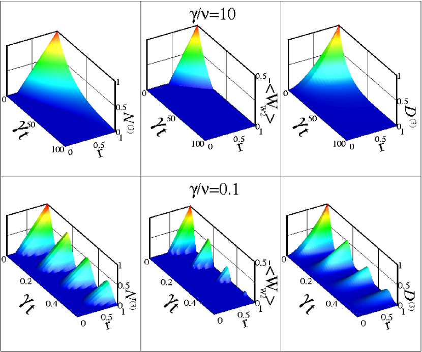
Figure 1: (Color online) Top panels: Negativity (left), opposite of the expectation value of the EW $\mathcal{W}_{W2}$ (center), and tripartite quantum discord (right) as a function of $\gamma t$ and the purity $r$ in the Markov regime with $\gamma/\nu$=10, when the three qubits, initially prepared in the state $\rho_{G}(0)$, are coupled to different sources of classical noise. Bottom panels: same as in the top panels in the non-Markov regime with $\gamma/\nu=0.1$.

In Fig. 1, we report $\mathcal{N}^{(3)}$, $-\langle\mathcal{W}_{W2}\rangle$, and $\mathcal{D}^{(3)}$ as a function of the time and the initial purity of the state for two different values of $\gamma/\nu$, namely 10 and 0.1, corresponding to the Markovian and non-Markovian dynamics of quantum correlations, respectively. In the first case, the RTN leads to a monotonic decay of entanglement and discord, while in the non-Markovian regime all quantities are damped oscillating functions of time and display sudden death and revival phenomena. Now let us compare qualitatively the behavior of the three estimators of quantum correlations. Even if the tripartite negativity and quantum discord present substantially the same qualitative behavior, nevertheless we find that $\mathcal{D}^{(3)}$ can take non-vanishing values in regions whereas $\mathcal{N}^{(3)}$ is zero. As it can clearly be seen in the non-Markovian regime, the peaks of the tripartite negative found at a given value of $\gamma t$ decrease for smaller $r$’s at higher rate than the corresponding peaks of the tripartite discord, and, as consequence vanish at smaller values of the purity of initial state. Such a behavior results to be consistent with was found in bipartite systems of initially entangled qubits evolving under local decohering channels where separable states can exhibit nonzero discord Mazzola et al. (2010); Werlang et al. (2009b); Fanchini et al. (2010). On the other hand, the entanglement and quantum correlations quantified in terms of $\mathcal{N}^{(3)}$ and $\mathcal{D}^{(3)}$ result to be higher, both in Markovian and non-Markovian regime, than the one detected by the tripartite entanglement witnesses.

IV.1.2 Common Environment

Now let us evaluate the dynamics of the quantum correlations initially present in the state $\rho_{G}(0)$ when the three qubits are coupled to a common source of RTN. The time-evolved tripartite negativity and expectation value of the witness $\mathcal{W}_{W2}$ can be expressed as:

$$\mathcal{N}^{(3)}(t)=\frac{1}{4}\max{\left[0,2r\sqrt{2\left(G^{2}_{4}(t)+1\right)}-(1-r)\right]}$$

$$\textrm{Tr}[{\rho}_{G}(t)\mathcal{W}_{W2}]=-\frac{1}{2}\left[\frac{3}{4}rG_{4}(t)-\left(\frac{3}{4}-r\right)\right].$$ (29)

It is worth noting that, unlike the case of local system-environment interaction, here quantum correlations are not totally destroyed at long times. Indeed, the asymptotic forms of Eqs. (IV.1.2), holding for any degree of qubit-environment coupling, are given by

$$\lim_{t\rightarrow\infty}\mathcal{N}^{(3)}(t)=\frac{1}{4}\max{\left[0,(2\sqrt{2}+1)r-1\right]}$$

$$-\lim_{t\rightarrow\infty}\textrm{Tr}[{\rho}_{G}(t)\mathcal{W}_{W2}]=\left(\frac{r}{2}-\frac{3}{8}\right).$$ (30)

This means that the saturation values of $\mathcal{N}^{(3)}$ and $\langle{\rho}_{G}\mathcal{W}_{W2}\rangle$ do not depend upon the parameter $\gamma$ that is, in terms, upon the Markovianity of the regimes. For an initial state with purity $r$ greater than $3/4$, the entanglement quantified in terms of the negativity and that part of entanglement detectable by means of the witness $\mathcal{W}_{W2}$ do not vanish in the long time limit. The partial preservation of the entanglement can be ascribed to the indirect interaction among the qubits stemming from the coupling of the global system to a common noisy environment. Unlike the local system-environment interaction, here the environment is no longer only the source of decohering effects, but also represents a sort of interaction mediator between the subsystem. Such an interaction somehow hinders the destruction of quantum correlations. The survival of quantum correlations has already been observed for the bipartite entanglement of two-qubit systems interacting with quantum environments Maniscalco et al. (2008); Bellomo et al. (2008); Ma et al. (2012). When the purity ranges from $3/4$ to $1/(2\sqrt{2}+1)$, the residual amount of tripartite entanglement at large times as quantified by $\mathcal{N}^{(3)}$ is not detectable by means of the EW $\mathcal{W}_{W2}$.

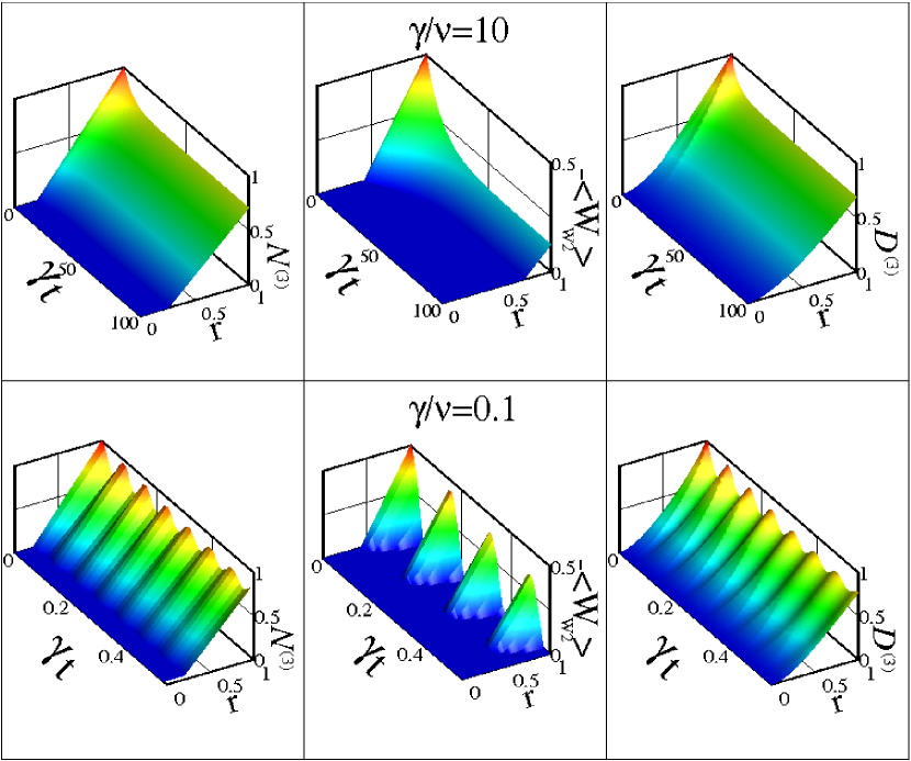
Figure 2: (Color online) Top panels: Negativity (left), opposite of the expectation value of EW $\mathcal{W}_{W2}$ (center), and tripartite quantum discord (right) as a function of $\gamma t$ and the purity $r$ in the Markov regime with $\gamma/\nu$=10, when the three qubits, initially prepared in the state $\rho_{GHZ}$, are coupled to a common source of classical noise. Bottom panels: same as in the top panels in the non-Markov regime with $\gamma/\nu=0.1$.

As shown in Fig. 2, also the tripartite quantum discord can survive the decohering effects due to the RTN. In the Markovian regime, we find that all the estimators decay monotonically with time until they reach the corresponding saturation values depending upon $r$. In the non-Markovian dynamics, both $\mathcal{N}^{(3)}$ and $\mathcal{D}^{(3)}$ exhibit damped oscillations but no sudden death of the correlations occurs for not-separable initial states. Indeed, the indirect interaction among the qubits not only counteracts the total suppression of of negativity and discord at long times but also prevents the disappearance of quantum correlations at finite times. The survival of $\mathcal{N}^{(3)}$ and $\mathcal{D}^{(3)}$ in the long time limit represents the major discrepancy with what was found in the two-qubit form of the model of Eqs. (15) and (16) Benedetti et al. (2012). There both bipartite entanglement and discord disappear at long times, regardless the local or non-local character of the interaction among the qubits and the environment.

Finally, the time behavior exhibited by the detectable entanglement in the non-Markovian regime appears to be peculiar. Indeed, the expectation value of the EW $\mathcal{W}_{W2}$ takes positive or null values at finite times in correspondence of the non-vanishing minima of the tripartite negativity. This implies that the suppression of the sudden death of entanglement cannot be detected while, as indicated by Eqs.(IV.1.2), the long-time entanglement protection can successfully be revealed.

IV.2 W-type states

IV.2.1 Different Environments

The dynamics of the quantum correlations, initially present in the state $\rho_{W}(0)$ of Eq. (27), is here analyzed for the case of qubit locally interacting with their environments. Unlike GHZ-type states discussed in the previous section, the tripartite negativity can not be put in a compact analytical form, while the expectation value of the EW $\mathcal{W}_{W1}$ can be expressed as:

$$\textrm{Tr}[{\rho}_{W}(t)\mathcal{W}_{W1}]=$$ (31)

$$-\frac{1}{24}\left[r\left(7G^{3}_{2}(t)+5G^{2}_{2}(t)+5G_{2}(t)+4\right)-13\right].$$

At the initial time for $r$=1, the expectation value of $\mathcal{W}_{W1}$ is $-1/3$, and the tripartite negativity is equal to 0.94. The EW detects entanglement when $r>13/21$, while $\mathcal{N}^{(3)}$ is nonzero for $r>0.2096$.

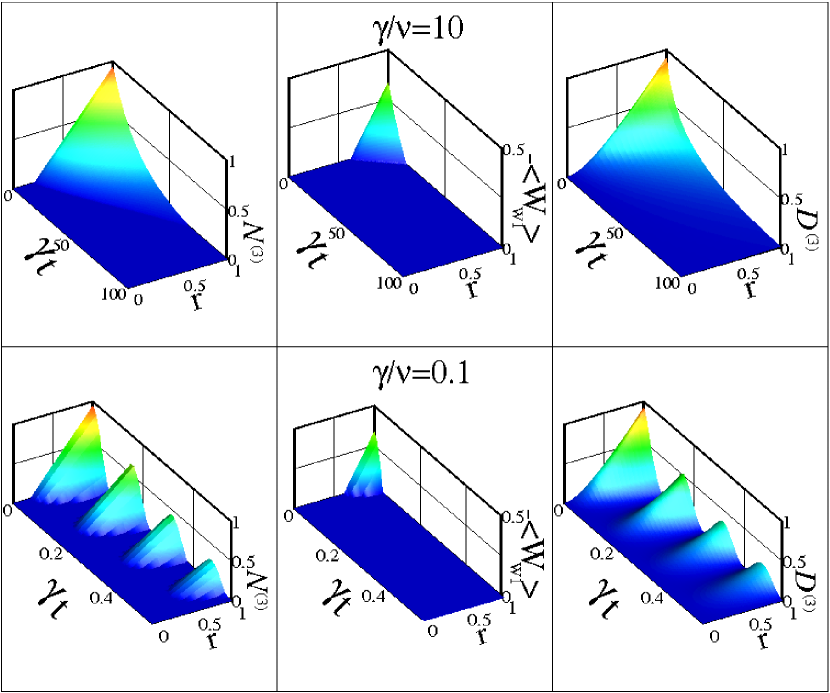
Figure 3: (Color online) Top panels: Negativity (left), opposite of the expectation value of EW $\mathcal{W}_{W1}$ (center), and tripartite quantum discord (right) as a function of $\gamma t$ and the purity $r$ in the Markov regime with $\gamma/\nu$=10, when the three qubits, initially prepared in the state $\rho_{W}(0)$, are coupled to different sources of classical noise. Bottom panels: same as in the top panels in the non-Markovian regime with $\gamma/\nu=0.1$.

Fig. 3 displays the tripartite negativity, the detectable entanglement and the discord as a function of time and initial purity of the state for two different values of $\gamma/\nu$, corresponding to Markov and non-Markov regime. In the first case, we find again the monotonic decay of $\mathcal{N}^{(3)}$ and $\mathcal{D}^{(3)}$ both vanishing at very long times. On the other hand the witness $\mathcal{W}_{W1}$ turns out to be unable to detect entanglement after a finite time. In the non-Markovian dynamics both the tripartite negativity and quantum discord exhibit revivals and sudden death phenomena, while the entanglement detectable by means of $\mathcal{W}_{W1}$ still decays monotonically with time and vanishes at short times. Also for this qubits configuration, the state can be separable even with a non-zero discord.

IV.2.2 Common Environment

Finally, we estimate the time evolution of the quantum correlations when the three qubits, initially set in the state $\rho_{W}(0)$, are subject to the decohering effects of a common source of RTN. The expectation value of the EW $\mathcal{W}_{W1}$ takes the form

$$\textrm{Tr}[{\rho}_{W}(t)\mathcal{W}_{W1}]=$$ (32)

$$-\left[\frac{r}{32}\left(9G_{6}(t)+6G_{4}(t)+7G_{2}(t)+6\right)-\frac{13}{24}\right].$$

Unlike what was found in the previous section, at long times entanglement cannot be detected independently from the value of $r$.

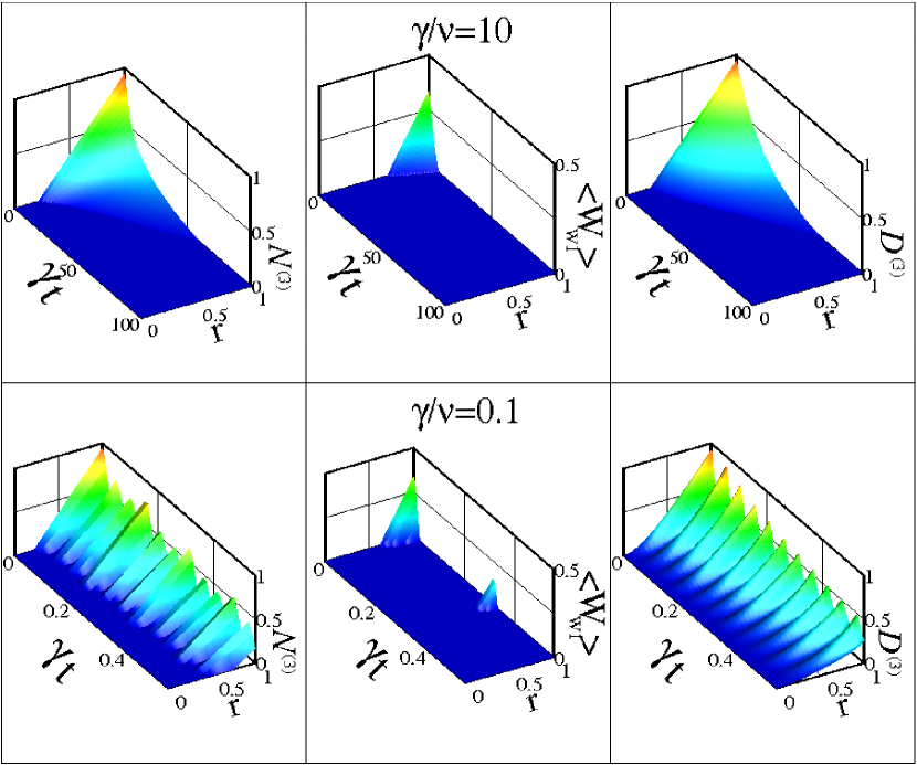
Figure 4: (Color online) Top panels: Negativity (left), opposite of the expectation value of EW $\mathcal{W}_{W1}$ (center), and tripartite quantum discord (right) as a function of $\gamma t$ and the purity $r$ in the Markov regime with $\gamma/\nu$=10, when the three qubits, initially prepared in the state $\rho_{W}$, are coupled to a common source of classical noise. Bottom panels: same as in the top panels in the non-Markovian regime with $\gamma/\nu=0.1$.

As it can be seen from Fig. 4, in the Markovian dynamics, the usual decay of quantum correlations is observed with tripartite negativity and quantum discord vanishing at long times. When the non Markovian dynamics is examined, $\mathcal{N}^{(3)}$ and $\mathcal{D}^{(3)}$ show damped oscillations without sudden death phenomena, even if they vanish in the long time limit (not displayed in the bottom panels of Fig. 4). On the other hand, a revival and sudden death of the detectable entanglement are observed. These results together with the ones shown in the previous subsection clearly indicate that the quantum correlations initially present in the W-type states are less robust than those of the GHZ-type states. Indeed, both tripartite entanglement and quantum discord of the state $\rho_{W}(0)$ are completely suppressed not only in the case of subsystems each locally coupled to its environment but also for non-local system-environment coupling.

V Conclusions

Recently, a number of theoretical works examined the dynamics of non-classical correlations in tripartite systems coupled to external environments characterized by different memory properties  Casagrande et al. (2009); Altintas and Eryigit (2010); Man et al. (2010); Anza et al. (2010); An et al. (2011); Siomau and Fritzsche (2010); Siomau (2012); Ma et al. (2010); Ann and Jaeger (2008); Liu et al. (2010); Weinstein (2009, 2010); Grimsmo et al. (2012). While different approaches have been adopted to estimate entanglement Casagrande et al. (2009); *Altintas; *Zhong-Xiao; *Anza; An et al. (2011); Siomau and Fritzsche (2010); *Siomau2; Weinstein (2009, 2010) and Bell non-locality Ma et al. (2010); Ann and Jaeger (2008); Liu et al. (2010), few studies focus on the time evolution of tripartite quantum correlations in terms of quantum discord Grimsmo et al. (2012).

In this paper, we address the dynamics of quantum correlations in a model consisting of three initially entangled qubits, not interacting among each other and coupled to different sources or to a common source of classical RTN. Specifically, two initial configurations have been considered, namely GHZ and W Werner-type states. Unlike previous analyses Siomau and Fritzsche (2010); Ann and Jaeger (2008); Altintas and Eryigit (2010); Liu et al. (2010); Ma et al. (2010); Weinstein (2009), here we have provided an estimate of the tripartite quantum discord by using the approach recently introduced in Ref. Giorgi et al. (2011) which allows one to quantify the amount of genuine tripartite quantum correlations of the system. These have then been compared with the entanglement evaluated by means of the tripartite negativity and with the detection ability of suitable EWs.

Our results show that both entanglement and quantum discord are strongly affected not only by the initial configuration of the qubits but also by the local or non-local nature of the system-environment interaction. In particular, for a GHZ-type initial state the indirect interaction between the qubits due to their coupling to a common source of RTN allows for a long-time tripartite entanglement and quantum discord preservation, regardless the Markov or non-Markov character of the environment itself. Furthermore, we find that the survived entanglement can be detected by means of the witnesses. On the other hand, quantum correlations are completely destroyed when the subsystems are coupled to different environments. The survival of entanglement and quantum discord and the disappearance of sudden death phenomena, which have already been observed in a number of bipartite systems interacting with quantum environments Maniscalco et al. (2008); Bellomo et al. (2008); Ma et al. (2012) are here closely related to the tripartite nature of the system. Indeed, in the two-qubit model analogous to the one here investigated the number of quantum correlations vanish in the long time limit under any condition Benedetti et al. (2012). By using approaches already used elsewhere De et al. (2011); Falci et al. (2005); Kuopanportti et al. (2008); Bergli et al. (2009), it could certainly be of interest to extend our investigation to the case of $1/f^{\alpha}$ noises stemming from a collection of random telegraph sources with different switching rates. So, we could verify the survival of quantum correlations when a large number of decoherence channels is considered.

In the other initial configuration, that is the qubits prepared in a W Werner-type state, no preservation of quantum correlations is found. Specifically, some of the standard features of Markov and non-Markov regime are observed. Indeed, the former exhibits a monotonic decay of quantum correlation while in the latter sudden death and revival phenomena occur only when the qubits are locally coupled to different sources of RTN. Anyway, both the entanglement and quantum discord of W Werner-type state turn out to be less robust than those of the GHZ-type state.

Finally, the tripartite quantum discord deserves a brief comment. It almost shows the same qualitative behavior of the negativity for all the physical conditions examined. Nevertheless, in agreement with what was previously found in bipartite systems Mazzola et al. (2010); Werlang et al. (2009b); Fanchini et al. (2010); Ali et al. (2010), the amount of tripartite quantum correlations quantified by discord can be different from zero for states without entanglement. From this point of view, our analysis seems to further validate the measure introduced in Ref. Giorgi et al. (2011) as a good estimator of the genuine tripartite quantum correlations which are not entanglement.

Appendix A Evaluation of the time-evolved states

Here, we give the explicit forms of the time-evolved state of the two different initial configurations of the qubits, namely GHZ and W Werner-type state, for the case of local and non-local system-environment interaction.

In order to evaluate the dynamics of the system, first we calculate the evolution of the initial state for a given choice of the noise parameter, as indicated in Eq. (17). Then, the obtained density matrix is averaged over noise (see Eq.(21)). For the input GHZ-type state $\rho_{G}(0)$ of Eq. (26), we find that, in the case of local system-environment coupling, the time-evolved density matrix of the system takes the form

$$\rho_{G}^{L}(t)=\left[\begin{array}[]{cccccccc}\alpha(t)&0&0&0&0&0&0&\sigma(t)\\ \vskip 6.0pt plus 2.0pt minus 2.0pt\cr 0&\theta(t)&0&0&0&0&\beta(t)&0\\ \vskip 6.0pt plus 2.0pt minus 2.0pt\cr 0&0&\theta(t)&0&0&\beta(t)&0&0\\ \vskip 6.0pt plus 2.0pt minus 2.0pt\cr 0&0&0&\theta(t)&\beta(t)&0&0&0\\ \vskip 6.0pt plus 2.0pt minus 2.0pt\cr 0&0&0&\beta(t)&\theta(t)&0&0&0\\ \vskip 6.0pt plus 2.0pt minus 2.0pt\cr 0&0&\beta(t)&0&0&\theta(t)&0&0\\ \vskip 6.0pt plus 2.0pt minus 2.0pt\cr 0&\beta(t)&0&0&0&0&\theta(t)&0\\ \vskip 6.0pt plus 2.0pt minus 2.0pt\cr\sigma(t)&0&0&0&0&0&0&\alpha(t)\end{array}\right],$$ (33)

with

$$\alpha(t)=\frac{1}{8}\left(1+3rG_{2}^{2}(t)\right),\quad\beta(t)=\frac{r}{8}\left(1-G_{2}^{2}(t)\right),$$

$$\theta(t)=\frac{1}{8}\left(1-rG_{2}^{2}(t)\right),\quad\textrm{and}\quad\sigma(t)=\frac{r}{8}\left(1+3G^{2}_{2}(t)\right).$$

On the other hand, for the case of non local qubit-environment interaction the dynamics of the system initially in $\rho_{G}(0)$ results into:

$$\rho_{G}^{NL}(t)=\left[\begin{array}[]{cccccccc}\frac{1}{8}+3\mu(t)&-\lambda(t)&-\lambda(t)&-\lambda(t)&-\lambda(t)&-\lambda(t)&-\lambda(t)&\frac{r}{8}+3\mu(t)\\ \vskip 6.0pt plus 2.0pt minus 2.0pt\cr-\lambda(t)&\frac{1}{8}-\mu(t)&\lambda(t)&\lambda(t)&\lambda(t)&\lambda(t)&\lambda(t)&-\lambda(t)\\ \vskip 6.0pt plus 2.0pt minus 2.0pt\cr-\lambda(t)&\lambda(t)&\frac{1}{8}-\mu(t)&\lambda(t)&\lambda(t)&\lambda(t)&\lambda(t)&-\lambda(t)\\ \vskip 6.0pt plus 2.0pt minus 2.0pt\cr-\lambda(t)&\lambda(t)&\lambda(t)&\frac{1}{8}-\mu(t)&\lambda(t)&\lambda(t)&\lambda(t)&-\lambda(t)\\ \vskip 6.0pt plus 2.0pt minus 2.0pt\cr-\lambda(t)&\lambda(t)&\lambda(t)&\lambda(t)&\frac{1}{8}-\mu(t)&\lambda(t)&\lambda(t)&-\lambda(t)\\ \vskip 6.0pt plus 2.0pt minus 2.0pt\cr-\lambda(t)&\lambda(t)&\lambda(t)&\lambda(t)&\lambda(t)&\frac{1}{8}-\mu(t)&\lambda(t)&-\lambda(t)\\ \vskip 6.0pt plus 2.0pt minus 2.0pt\cr-\lambda(t)&\lambda(t)&\lambda(t)&\lambda(t)&\lambda(t)&\lambda(t)&\frac{1}{8}-\mu(t)&-\lambda(t)\\ \vskip 6.0pt plus 2.0pt minus 2.0pt\cr\frac{r}{8}+3\mu(t)&-\lambda(t)&-\lambda(t)&-\lambda(t)&-\lambda(t)&-\lambda(t)&-\lambda(t)&\frac{1}{8}+3\mu(t)\end{array}\right],$$ (35)

where

$$\mu(t)=\frac{r}{16}\left(1+G_{4}(t)\right),\quad\textrm{and}\quad\lambda(t)=\frac{r}{16}\left(1-G_{4}(t)\right).$$ (36)

These results clearly show that the form of the time-evolved density matrix of three qubits initially in a GHZ-type state depend upon the local or non-local nature of the system-environment coupling.

Now let us focus on the time evolution of the system initially prepared in the W-type state $\rho_{W}(0)$ given in Eq. (27). When each qubit interacts locally with its environment, the density matrix of the system at time $t$ takes the form:

$$\rho_{W}^{L}(t)=\left[\begin{array}[]{cccccccc}\frac{\kappa(t)}{8}+\varsigma&0&0&\frac{\kappa(t)}{12}&0&\frac{\kappa(t)}{12}&\frac{\kappa(t)}{12}&0\\ \vskip 6.0pt plus 2.0pt minus 2.0pt\cr 0&\frac{\tau(t)}{24}+\varsigma&\frac{\iota(t)}{12}&0&\frac{\iota(t)}{12}&0&0&\frac{\chi(t)}{12}\\ \vskip 6.0pt plus 2.0pt minus 2.0pt\cr 0&\frac{\iota(t)}{12}&\frac{\tau(t)}{24}+\varsigma&0&\frac{\iota(t)}{12}&0&0&\frac{\chi(t)}{12}\\ \vskip 6.0pt plus 2.0pt minus 2.0pt\cr\frac{\kappa(t)}{12}&0&0&\frac{\xi(t)}{24}+\varsigma&0&\frac{\varphi(t)}{12}&\frac{\varphi(t)}{12}&0\\ \vskip 6.0pt plus 2.0pt minus 2.0pt\cr 0&\frac{\iota(t)}{12}&\frac{\iota(t)}{12}&0&\frac{\tau(t)}{24}+\varsigma&0&0&\frac{\chi(t)}{12}\\ \vskip 6.0pt plus 2.0pt minus 2.0pt\cr\frac{\kappa(t)}{12}&0&0&\frac{\varphi(t)}{12}&0&\frac{\xi(t)}{24}+\varsigma&\frac{\varphi(t)}{12}&0\\ \vskip 6.0pt plus 2.0pt minus 2.0pt\cr\frac{\kappa(t)}{12}&0&0&\frac{\varphi(t)}{12}&0&\frac{\varphi(t)}{12}&\frac{\xi(t)}{24}+\varsigma&0\\ \vskip 6.0pt plus 2.0pt minus 2.0pt\cr 0&\frac{\chi(t)}{12}&\frac{\chi(t)}{12}&0&\frac{\chi(t)}{12}&0&0&\frac{\chi(t)}{8}+\varsigma\end{array}\right],$$ (37)

where

$$\kappa(t)=r\big{(}1+G_{2}(t)\big{)}^{2}\big{(}1-G_{2}(t)\big{)},\quad\varsigma=\frac{1}{8}(1-r),\quad\chi(t)=r\big{(}1-G_{2}(t)\big{)}^{2}\big{(}1+G_{2}(t)\big{)},$$

$$\tau(t)=r\big{(}1+G_{2}(t)\big{)}\big{[}\big{(}1+G_{2}(t)\big{)}^{2}+2\big{(}1-G_{2}(t)\big{)}^{2}\big{]},\quad\iota(t)=r\big{(}1+G_{2}(t)\big{)}\left(1+G_{2}^{2}(t)\right),$$

$$\ \xi(t)=r\big{(}1-G_{2}(t)\big{)}\big{[}2\big{(}1+G_{2}(t)\big{)}^{2}+\big{(}1-G_{2}(t)\big{)}^{2}\big{]},\quad\varphi(t)=r\big{(}1-G_{2}(t)\big{)}\left(1+G_{2}^{2}(t)\right).$$

When all the three qubits are coupled to a common source of RTN, the time-evolved state of the system can written as:

$$\rho_{W}^{NL}(t)=\left[\begin{array}[]{cccccccc}\frac{1}{8}+\Lambda(t)&0&0&\Xi(t)&0&\Xi(t)&\Xi(t)&0\\ \vskip 6.0pt plus 2.0pt minus 2.0pt\cr 0&\frac{1}{8}+\Upsilon(t)&\Omega(t)&0&\Omega(t)&0&0&\Gamma(t)\\ \vskip 6.0pt plus 2.0pt minus 2.0pt\cr 0&\Omega(t)&\frac{1}{8}+\Upsilon(t)&0&\Omega(t)&0&0&\Gamma(t)\\ \vskip 6.0pt plus 2.0pt minus 2.0pt\cr\Xi(t)&0&0&\frac{1}{8}+\Phi(t)&0&\Delta(t)&\Delta(t)&0\\ \vskip 6.0pt plus 2.0pt minus 2.0pt\cr 0&\Omega(t)&\Omega(t)&0&\frac{1}{8}+\Upsilon(t)&0&0&\Gamma(t)\\ \vskip 6.0pt plus 2.0pt minus 2.0pt\cr\Xi(t)&0&0&\Delta(t)&0&\frac{1}{8}+\Phi(t)&\Delta(t)&0\\ \vskip 6.0pt plus 2.0pt minus 2.0pt\cr\Xi(t)&0&0&\Delta(t)&0&\Delta(t)&\frac{1}{8}+\Phi(t)&0\\ \vskip 6.0pt plus 2.0pt minus 2.0pt\cr 0&\Gamma(t)&\Gamma(t)&0&\Gamma(t)&0&0&\frac{1}{8}+\Psi(t)\end{array}\right],$$ (38)

with

$$\Lambda(t)=r\left(\frac{1}{16}+\frac{3G_{2}(t)}{32}-\frac{3G_{4}(t)}{16}-\frac{3G_{6}(t)}{32}\right),\quad\Xi(t)=r\left(\frac{1}{16}+\frac{3G_{2}(t)}{32}-\frac{G_{4}(t)}{16}-\frac{3G_{6}(t)}{32}\right),$$

$$\Upsilon(t)=r\left(\frac{-1}{48}+\frac{7G_{2}(t)}{96}+\frac{G_{4}(t)}{16}+\frac{3G_{6}(t)}{32}\right),\quad\Omega(t)=r\left(\frac{5}{48}+\frac{7G_{2}(t)}{96}+\frac{G_{4}(t)}{16}+\frac{3G_{6}(t)}{32}\right),$$

$$\Gamma(t)=r\left(\frac{1}{16}-\frac{3G_{2}(t)}{32}-\frac{G_{4}(t)}{16}+\frac{3G_{6}(t)}{32}\right),\quad\Phi(t)=r\left(\frac{-1}{48}-\frac{7G_{2}(t)}{96}+\frac{G_{4}(t)}{16}-\frac{3G_{6}(t)}{32}\right),$$

$$\Delta(t)=r\left(\frac{5}{48}-\frac{7G_{2}(t)}{96}+\frac{G_{4}(t)}{16}-\frac{3G_{6}(t)}{32}\right),\quad\Psi(t)=r\left(\frac{1}{16}-\frac{3G_{2}(t)}{32}-\frac{3G_{4}(t)}{16}+\frac{3G_{6}(t)}{32}\right).$$

Unlike the GHZ Werner-type state, we note that in this case the time-evolved density matrix of the system takes the same form for local and non-local system-environment interaction. Indeed, in both the matrices of Eqs. (37) and (38) the diagonal 4$\times$4 subblocks have an X shape, while in the antidiagonal ones the diagonal and antidiagonal elements are zero.

References

- Nielsen and Chuang (2000) M. Nielsen and I. Chuang, Quantum Computation and Quantum Information (Cambridge University Press, Cambridge, England, 2000).
- Joos et al. (2003) E. Joos, H. Zeh, C. Kiefer, D. Giulini, J. Kupsch, and I. Stamatescu, Decoherence and the Appearance of a Classical World in Quantum Theory (Springer, Berlin, 2003).
- Yu and Eberly (2004) T. Yu and J. H. Eberly, Phys. Rev. Lett. 93, 140404 (2004).
- Bellomo et al. (2008) B. Bellomo, R. Lo Franco, S. Maniscalco, and G. Compagno, Phys. Rev. A 78, 060302 (2008).
- Maniscalco et al. (2008) S. Maniscalco, F. Francica, R. L. Zaffino, N. Lo Gullo, and F. Plastina, Phys. Rev. Lett. 100, 090503 (2008).
- An et al. (2011) N. B. An, J. Kim, and K. Kim, Phys. Rev. A 84, 022329 (2011).
- Buscemi et al. (2009) F. Buscemi, P. Bordone, and A. Bertoni, J. Phys. Cond. Matter 21, 305303 (2009).
- Buscemi et al. (2010) F. Buscemi, P. Bordone, and A. Bertoni, Phys. Rev. B 81, 045312 (2010).
- Buscemi (2011) F. Buscemi, Phys. Rev. A 83, 012302 (2011).
- Bellomo et al. (2007) B. Bellomo, R. Lo Franco, and G. Compagno, Phys. Rev. Lett. 99, 160502 (2007).
- Casagrande et al. (2009) F. Casagrande, A. Lulli, and M. G. A. Paris, Phys. Rev. A 79, 022307 (2009).
- Altintas and Eryigit (2010) F. Altintas and R. Eryigit, Physics Letters A 374, 4283 (2010).
- Man et al. (2010) Z.-X. Man, Y.-J. Xia, and N. B. An, New Journal of Physics 12, 033020 (2010).
- Anza et al. (2010) F. Anza, B. Militello, and A. Messina, J. Phys. B 43, 205501 (2010).
- Siomau and Fritzsche (2010) M. Siomau and S. Fritzsche, Phys. Rev. A 82, 062327 (2010).
- Siomau (2012) M. Siomau, Journal of Physics B: Atomic, Molecular and Optical Physics 45, 035501 (2012).
- Ma et al. (2010) X. S. Ma, G. S. Liu, G. Zhao, and A. M. Wang, Physica A 389, 5103 (2010).
- Ann and Jaeger (2008) K. Ann and G. Jaeger, Physics Letters A 372, 6853 (2008).
- Liu et al. (2010) B.-Q. Liu, B. Shao, and J. Zou, Physics Letters A 374, 1970 (2010).
- Weinstein (2009) Y. S. Weinstein, Phys. Rev. A 79, 012318 (2009).
- Weinstein (2010) Y. S. Weinstein, Phys. Rev. A 82, 032326 (2010).
- Acin et al. (2000) A. Acin, A. Andrianov, L. Costa, E. Jane, J. I. Latorre, and R. Tarrach, Phys. Rev. Lett. 85, 1560 (2000).
- Ollivier and Zurek (2001) H. Ollivier and W. H. Zurek, Phys. Rev. Lett. 88, 017901 (2001).
- Henderson and Vedral (2001) L. Henderson and V. Vedral, J. Phys. A 34, 6899 (2001).
- Werlang et al. (2009a) T. Werlang, S. Souza, F. F. Fanchini, and C. J. Villas Boas, Phys. Rev. A 80, 024103 (2009a).
- Mazzola et al. (2010) L. Mazzola, J. Piilo, and S. Maniscalco, Phys. Rev. Lett. 104, 200401 (2010).
- Fanchini et al. (2010) F. F. Fanchini, T. Werlang, C. A. Brasil, L. G. E. Arruda, and A. O. Caldeira, Phys. Rev. A 81, 052107 (2010).
- Datta et al. (2008) A. Datta, A. Shaji, and C. M. Caves, Phys. Rev. Lett. 100, 050502 (2008).
- Lanyon et al. (2008) B. P. Lanyon, M. Barbieri, M. P. Almeida, and A. G. White, Phys. Rev. Lett. 101, 200501 (2008).
- Kaszlikowski et al. (2008) D. Kaszlikowski, A. Sen(De), U. Sen, V. Vedral, and A. Winter, Phys. Rev. Lett. 101, 070502 (2008).
- Rulli and Sarandy (2011) C. C. Rulli and M. S. Sarandy, Phys. Rev. A 84, 042109 (2011).
- Chakrabarty et al. (2011) I. Chakrabarty, P. Agrawal, and A. Pati, Eur. Phys. J. D 65, 605 (2011).
- Grimsmo et al. (2012) A. L. Grimsmo, S. Parkins, and B.-S. K. Skagerstam, Phys. Rev. A 86, 022310 (2012).
- Giorgi et al. (2011) G. L. Giorgi, B. Bellomo, F. Galve, and R. Zambrini, Phys. Rev. Lett. 107, 190501 (2011).
- Zhao et al. (2012) L. Zhao, X. Hu, R.-H. Yue, and H. Fan, (2012), arXiv:1206.1908 [quant-ph] .
- Zhou et al. (2010) D. Zhou, A. Lang, and R. Joynt, Quantum Information Processing 9, 727 (2010).
- De et al. (2011) A. De, A. Lang, D. Zhou, and R. Joynt, Phys. Rev. A 83, 042331 (2011).
- Möttönen et al. (2006) M. Möttönen, R. de Sousa, J. Zhang, and K. B. Whaley, Phys. Rev. A 73, 022332 (2006).
- Bordone et al. (2012) P. Bordone, F. Buscemi, and C. Benedetti, Fluctuation and Noise Letters 11, 1242003 (2012).
- Benedetti et al. (2012) C. Benedetti, F. Buscemi, P. Bordone, and M. G. A. Paris, (2012), arXiv:1209.4201 [quant-ph] .
- Saira et al. (2007) O.-P. Saira, V. Bergholm, T. Ojanen, and M. Möttönen, Phys. Rev. A 75, 012308 (2007).
- Lo Franco et al. (2012) R. Lo Franco, B. Bellomo, E. Andersson, and G. Compagno, Phys. Rev. A 85, 032318 (2012).
- Sabin and Garcia-Alcaine (2008) C. Sabin and G. Garcia-Alcaine, Eur. Phys. J. D 48, 435 (2008).
- Buscemi and Bordone (2011) F. Buscemi and P. Bordone, Phys. Rev. A 84, 022303 (2011).
- Benedetti et al. (2012) C. Benedetti, F. Buscemi, and P. Bordone, Phys. Rev. A 85, 042314 (2012).
- Bergli et al. (2009) J. Bergli, Y. M. Galperin, and B. L. Altshuler, New Journal of Physics 11, 025002 (2009).
- Werlang et al. (2009b) T. Werlang, S. Souza, F. F. Fanchini, and C. J. Villas Boas, Phys. Rev. A 80, 024103 (2009b).
- Ma et al. (2012) J. Ma, Z. Sun, X. Wang, and F. Nori, Phys. Rev. A 85, 062323 (2012).
- Falci et al. (2005) G. Falci, A. D’Arrigo, A. Mastellone, and E. Paladino, Phys. Rev. Lett. 94, 167002 (2005).
- Kuopanportti et al. (2008) P. Kuopanportti, M. Möttönen, V. Bergholm, O.-P. Saira, J. Zhang, and K. B. Whaley, Phys. Rev. A 77, 032334 (2008).
- Ali et al. (2010) M. Ali, A. R. P. Rau, and G. Alber, Phys. Rev. A 81, 042105 (2010).