An Analytical Model of Radiation-Induced Charge Transfer Inefficiency for CCD Detectors

Abstract

The European Space Agency’s Gaia mission is scheduled for launch in 2013. It will operate at L2 for 5 years, rotating slowly to scan the sky so that its two optical telescopes will repeatedly observe more than one billion stars. The resulting data set will be iteratively reduced to solve for the position, parallax and proper motion of every observed star. The focal plane contains 106 large area silicon CCDs continuously operating in a mode where the line transfer rate and the satellite rotation are in synchronisation.

One of the greatest challenges facing the mission is radiation damage to the CCDs which will cause charge deferral and image shape distortion. This is particularly important because of the extreme accuracy requirements of the mission. Despite steps taken at hardware level to minimise the effects of radiation, the residual distortion will need to be calibrated during the pipeline data processing. Due to the volume and inhomogeneity of data involved, this requires a model which describes the effects of the radiation damage which is physically realistic, yet fast enough to implement in the pipeline. The resulting charge distortion model was developed specifically for the Gaia CCD operating mode. However, a generalised version is presented in this paper and this has already been applied in a broader context, for example to investigate the impact of radiation damage on the Euclid dark-energy mission data.

1 Introduction

Gaia is a European Space Agency mission, planned for launch in 2013, which aims to perform global astrometry on approximately one percent of the estimated galactic stellar population to unprecedented accuracy(see Perryman et al., 2001; Lindegren et al., 2008). The scanning satellite will operate at the earth/moon-sun Lagrangian point for 5 years, rotating slowly so that its two optical telescopes will repeatedly observe more than a thousand million stars. The resulting dataset will be iteratively reduced to solve for the position, parallax and proper motion of every observed star (additionally, dispersed spectra will be obtained for a subset of these objects). The mission requirements for the astrometric precision are in the micro-arcsecond ($\mu$as) regime. These stringent astrometric requirements translate into milli-pixel-level accuracies on the stellar image location per individual CCD observation, e.g., Prod’homme et al. (2011).

The Gaia focal plane (e.g., de Bruijne et al., 2010), the largest to date to be sent to space, contains 106 large-area silicon CCDs continuously operating in Time Delay Integration (TDI) mode at a line-clocking rate which is in synchronisation with the satellite rotation rate. Each CCD was custom-made by e2v technologies for the Gaia project and consists of 4500 $\times$ 1966 (parallel $\times$ serial) pixels of physical dimension 10 $\times$ 30 $\mu\mathrm{m}$ (for further detail see Prod’homme et al., 2011). Due to a combination of the large number of transfers of the charge packet (parallel) and fast clocking speed (serial), the limits placed on the amount of radiation shielding due to mass-budget constraints, the predicted radiation environment at L2, and the extreme accuracy requirements on the image location estimates, Charge Transfer Inefficiency (CTI) of the CCDs was identified as a challenge for the Gaia mission at an early stage.

CTI during the transfer of electron packets from pixel to pixel is due to the stochastic capture and release of signal electrons into and out of trapping sites in the silicon lattice structure. This will have two major effects upon Gaia data:

1. the removal of charge from the signal within the windowed image resulting in a loss of signal and a corresponding irretrievable degradation in the signal-to-noise ratio.

2. A distortion and centroid shift of the image due to the emission of electrons into charge packets different to those which they were captured from.

These effects are schematically illustrated in Figure 1 and Figure 2.

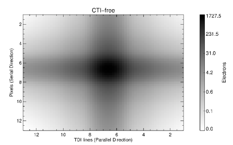
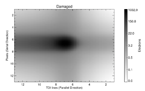
Figure 1: Upper Panel: Simulation of a 5 $\times$ oversampled image in the abscence of CTI. Lower Panel: The effect of parallel CTI on the image in the top panel. The CTI effect was simulated using the model described in this paper. Note that unrealistic model parameters were chosen in order to exaggerate the effect for clarity. The readout direction is to the right.

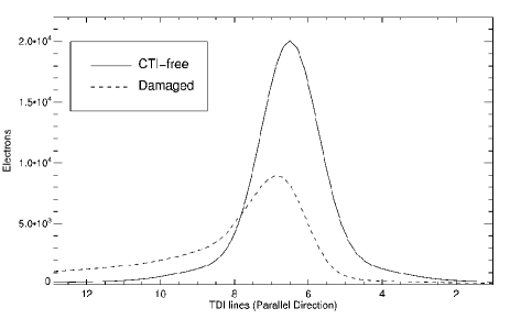
Figure 2: Simulation of a 5 $\times$ oversampled image that is binned in the serial direction (the vast majority of Gaia observations will have on-chip binning applied in the serial direction). The effect of parallel CTI on the image is plotted in dashed. The CTI effect was simulated using the model described in this paper. Note that unrealistic model parameters were chosen in order to exaggerate the effect for clarity. The readout direction is to the right.

The distortion of the image shape, if uncalibrated, will introduce a systematic bias on the measured image location and result in a degradation of the end-of-mission astrometric accuracies from $\mu$as to mas levels. Indeed, based on simulations, Prod’homme et al. (2011) estimate a bias of up to $\sim 0.2$ pixels in the CCD location measurement ($\sim 10$ mill-arcseconds) as a result of CTI in the uncalibrated case, which is in agreement with on-ground test data. The main reasons that the effect on the performance is so large is due to the harsh radiation environment at L2 (dominated by energetic solar protons) and the stringent mission requirements on the image location measurements. It is well established that the interaction of high-energy protons with CCD devices can result in displacement damage in the silicon structure and the generation of ‘new’ energy levels in the semiconductor band-gap, otherwise known as ‘traps’, that can capture and, after some time, release the electrons. These radiation-induced traps dramatically increase the CTI of the detector and raise the radiation issue to being mission-critical in the absence of adequate mitigation. For further discussion of radiation-induced CTI see Hardy et al. (1998); Janesick (2001).

In order to minimise the CTI effects, a number of hardware solutions has been implemented for Gaia. For example, a mechanism for the periodic injection of charge into lines of the CCD in order to keep traps filled has been implemented (charge injection). A supplementary buried channel has also been incorporated into the CCD design to funnel charge from small electron packets into a smaller pixel volume during transfer in order to minimise the number of traps that will be encountered at low signals (for further reading see Seabroke et al., 2013). However, in order for Gaia to meet its scientific requirements, a calibration of the residual effects of radiation-induced CTI is mandatory.

The entire set of Gaia observations will be used to solve for the astrometric parameters of each star, as well as the satellite attitude parameters and calibration parameters using the Astrometric Global Iterative Solution (AGIS) described in Lindegren et al. (2012). Radiation-induced distortions of the images are a source of systematic error which, given a suitable model, could be removed as part of the global solution. Therefore, the current baseline approach to tackle the calibration of radiation-induced trapping effects in Gaia data is through the application of a forward modelling technique in the pipeline processing. Under this scheme, the parameters of the CTI-free image (location and integrated flux) and the parameters of a model which can replicate the CTI effects on the CTI-free image are iteratively adjusted until the predicted distorted image best matches the observed image. This approach requires a model that can replicate the distortion of a sampled image due to radiation-induced trapping effects, we call this a Charge Distortion Model (CDM). The forward-modelling approach is preferable to a corrective approach in order to preserve the noise properties of the data, as well as having the flexibility to treat dispersed spectra and non-point source objects in the same manner as isolated single stars in the data processing. However, the CDM must be realistic and flexible enough to reproduce the distortion effectively, whilst simultaneously being fast enough for implementation in the data processing pipeline. The CDM can be empirical and need not be based upon detailed physical modelling of electron trapping and release. However, any model based upon physical considerations is certain to be superior in terms of application over a broad parameter space using the fewest possible variables. Since computational speed is of high concern, the model need not treat individual pixel transfers, but instead, approximate the trapping and release during the transit of an entire CCD column (or, indeed, the readout register) in a single calculation. In order to treat the non-integrating (non-TDI) charge injection lines, transfer through the serial register and also for general applicability, the model should also have the capability to treat the charge transfer when the signal is non-integrating (imaging mode).

During the course of Gaia development and preparation studies, a great deal has been learned regarding the phenomenological interpretation of trapping, de-trapping and electron confinement from the very large to the very small signal regimes. Over the course of five radiation test campaigns, many datasets have been acquired in TDI mode using partially-irradiated Gaia CCDs in order to characterise the CTI effects. Monte-Carlo (e.g., Prod’homme et al., 2011) and analytical models have also been developed which go some way to reproducing Gaia radiation test data. However, the sub-pixel level Monte Carlo CCD models developed for Gaia are far too computationally expensive to be applied as a CDM in the forward modelling scheme which needs to run on $\sim 10^{12}$ separate CCD observations collected over the course of the mission In this paper, we present a model, based upon a physical understanding of trapping effects, but with some very significant simplifications such that it can be incorporated into the data processing pipeline. Further discussions and quantitative predictions on the performance of Gaia in the presence of CTI (including the use of this CDM for CTI-mitigation) can be found within Prod’homme et al. (2011) and Holl et al. (2012).

The paper is structured as follows. In Section 2 we address the constraints imposed on the model from the analysis of Gaia-specific test data acquired in TDI mode. The details of the model are then presented in Section 3. In Section 4 we show an overview of the application of the model to test data and, finally, in Section 5 we present our conclusions.

2 Background to the Model

The objective is to derive an analytical CDM that takes into account recent illumination and charge injection history and is based upon accepted physical theory, i.e. Shockley-Read-Hall theory (e.g., Hardy et al., 1998) and knowledge gained from Gaia testing. The first iteration of such a CDM was proposed by Lindegren (2008), however, his model is not based on physical theory and was always intended as a place-holder.

In order to apply the Shockley-Read-Hall equations it is necessary to model the volume and density of the electron packets as they move through the CCD. This will give the numbers of traps encountered by an electron packet according to the trap density, as well as the probability that a trap captures or releases an electron. In this respect, the models developed for Gaia fall into two broad categories: Confinement Volume (or volume driven) models and Density Distribution (or density driven) models.

CCD models usually consider electrons to be contained in charge packets resting in potential minima defined by the applied electrode potentials. The electron cloud is typically assumed to have a finite confinement volume which increases as more electrons are added. Hence a model such as:

$$\frac{V_{c}}{V_{g}} =\left(\frac{N_{e}}{FWC}\right)^{\beta}$$ (1)

might be adopted for the volume of the charge cloud ($V_{c}$), where $N_{e}$ is the number of electrons in a pixel, $FWC$ is the pixel $Full$ $Well$ $Capacity$ in electrons and $V_{g}$ is the assumed maximum geometrical volume that electrons can occupy within a pixel (i.e. the volume of the electron cloud when $N_{e}=FWC$). In most models, the value of $\beta$ would be assumed to be close to 1, the density of confined electrons would be almost constant and high enough for trapping within the electron packet volume to be considered instantaneous. We may refer to models with these properties as volume driven models where all vacant traps within the electron packet will capture an electron whilst those outside cannot, and the amount of trapping observed will be driven by the electron packet volume. Early models developed for Gaia were all volume driven. However, there was a major shortcoming of this assumption which causes them to fail for Gaia.

Volume driven models are unable to reproduce or to explain the observed effect that a small number of background electrons can have upon overall trap occupancy. It is observed that very low level optical background (fat zero) is able to suppress a disproportionate fraction of slow traps (e.g., Brown & van Leeuwen, 2008; Short, 2006). According to volume driven models, this would require that background electrons must occupy a volume many thousands of times larger than an equivalent number of signal electrons. In addition, Gaia testing clearly indicates that a diffuse optical background preferentially eliminates traps with long release time constants (slow traps) but does little or nothing to suppress faster traps. The effect of background upon the traps suggests that a different model must be applied allowing electrons to reach the traps in the first place. In other words, we must assume that $\beta$ in equation 1 is closer to 0 rather than 1 and that it is primarily the density of electrons rather than the volume which increases as more electrons are added. In this way, all electron packets will encounter a similar population of traps but the probability that a given trap captures an electron in a given time will depend upon the local electron density which increases with signal size.

3 Model Description

In this section we break down the model description into four differerent sections. We describe the modelling of the electron trapping in TDI mode, the trapping in imaging mode, electon release and, finally, the tracking of the trap occupancies as a function of time.

3.1 Electron trapping in TDI mode

3.1.1 Interaction volume

We take equation 1 as a starting point, noting that $\beta$ is not constrained to values close to 1 but may take any value between 0 and 1 allowing complete flexibility with regard to the question of volume or density driven models. Clearly, if $\beta$ is equal to 0 then $V_{c}=V_{g}$ is a constant. Only the electron density increases as electrons are added and trapping is entirely density driven. If $\beta$ is equal to 1 then $V_{c}$ grows linearly with $N_{e}$, electron density is constant and trapping is entirely driven by the interaction volume of the electrons with the traps. Figure 3 illustrates the variation of electron confinement volume, $V_{c}$ as a function of $N_{e}$ and $\beta$ (according to equation 1).

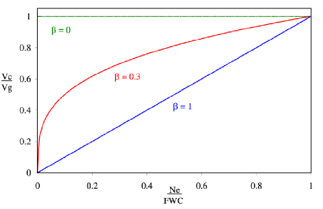
Figure 3: Variation of electron confinement volume, $V_{c}$ with number of electrons, $N_{e}$ according to equation 1.

Since we intend to treat the trapping along the column in a single step, we may derive the fraction of the total volume of silicon in the column that was “seen” by a given sample ($S$), by integrating equation 1 as the signal electrons accumulate along the CCD column from $N_{e}=0$ to $N_{e}=S$:

$$\frac{\mbox{volume that sees electrons}}{\mbox{volume of column}} =\frac{1}{S}\int_{0}^{S}\left(\frac{N_{e}}{FWC}\right)^{\beta}\,\mathrm{d}N_{e}$$

$$=\frac{1}{1+\beta}\left(\frac{S}{FWC}\right)^{\beta}$$ (2)

where it should be understood that $S$, the input to the CDM is the size of the sample (in electrons) that would be read out of the CCD in the absence of trapping, i.e. the un-distorted sample. Assuming that $N_{T}$ traps are distributed uniformly throughout the volume of the column, then the fraction of these traps with which the $S$ electrons can interact is equal to the interacting fraction of the column volume. However, if we assume that $N_{o}$ of the traps within the column are already occupied, then we can write the fraction of all traps in the column that will interact with the $S$ electrons and that are vacant:

$$F_{T} =\frac{\mbox{vacant traps that see electrons}}{\mbox{total number of traps}}$$

$$=\frac{1}{1+\beta}\left(\frac{S}{FWC}\right)^{\beta}-\frac{N_{o}}{N_{T}}$$ (3)

Similarly, we may write the fraction of signal electrons, $S$, that see vacant (rather than occupied) traps:

$$F_{e} =\frac{\mbox{electrons that see vacant traps}}{\mbox{total number of electrons}}$$

$$=\frac{\frac{1}{1+\beta}\left(\frac{S}{FWC}\right)^{\beta}-\frac{N_{o}}{N_{T}}}{\frac{1}{1+\beta}\left(\frac{S}{FWC}\right)^{\beta}}$$ (4)

If trapping were allowed to proceed until all of the vacant traps were occupied or all of the available electrons were captured, then the number of captures, $N_{c}$ would be equal to the number of available traps or the number of available electrons (whichever is fewer). This may be expressed:

$$N_{c}|_{t\rightarrow\infty} =\frac{N_{T}F_{T}SF_{e}}{N_{T}F_{T}+SF_{e}}$$

$$=\frac{N_{T}\left(\frac{1}{1+\beta}\left(\frac{S}{FWC}\right)^{\beta}-\frac{N_{o}}{N_{T}}\right)S\frac{\left(\frac{1}{1+\beta}\left(\frac{S}{FWC}\right)^{\beta}-\frac{N_{o}}{N_{T}}\right)}{\frac{1}{1+\beta}\left(\frac{S}{FWC}\right)^{\beta}}}{N_{T}\left(\frac{1}{1+\beta}\left(\frac{S}{FWC}\right)^{\beta}-\frac{N_{o}}{N_{T}}\right)+S\frac{\left(\frac{1}{1+\beta}\left(\frac{S}{FWC}\right)^{\beta}-\frac{N_{o}}{N_{T}}\right)}{\frac{1}{1+\beta}\left(\frac{S}{FWC}\right)^{\beta}}}$$

$$=\frac{\gamma S^{\beta}-N_{o}}{\gamma S^{\beta-1}+1}\qquad\mbox{where}\qquad\gamma=\frac{N_{T}}{\left(1+\beta\right)FWC^{\beta}}$$ (5)

When implementing the model, it is more general to use a trap density, $n_{t}$, rather than a number of traps in the column, $N_{T}$. Thus, substituting $N_{T}=2n_{t}V_{g}x$ where $x$ is the number of TDI transfers or the column length in pixels, we get:

$$\gamma=\frac{2n_{t}V_{g}x}{\left(1+\beta\right)FWC^{\beta}}$$ (6)

3.1.2 Finite trapping time

Equation 5 may be used to model electron trapping in TDI mode in the event that capture times are always short in relation to electron-trap interaction times (i.e. semi instantaneous trapping). However, it is well established through Gaia testing, that the very low electron densities being transferred in TDI mode give rise to electron capture times that are on the order of the pixel dwell time and it is therefore not appropriate to consider instantaneous trapping. Instead, we must evaluate the probability of electron capture according to electron density. In TDI mode the electron density is increasing as the signal integrates along the CCD column. Therefore, most Gaia models evaluate the probability of capture (and release) per line transfer or intra-pixel CCD phase (4 500 transfers or 18 000 phases, since each pixel contains four individual gate electrodes). However, for the purposes of this high speed model, we require an expression giving the column-averaged probability of capture for a transit as a function of (integrating) signal size and trap occupancy.

If we assume that traps in the CCD column interact with the electrons of a given sample for a period equal to half the TDI period ($t$) then the probability ($P_{c}$) that a vacant trap will capture an electron is:

$$P_{c}=1-\mbox{e}^{-\frac{t}{2\tau_{c}}}$$ (7)

where $\tau_{c}$ is the capture time constant:

$$\tau_{c}=\frac{1}{\sigma v_{t}n_{e}}$$ (8)

The quantity $\sigma$ is the trap capture cross-section, $n_{e}$ is the electron density in the vicinity of the trap and $v_{t}$ is the electron thermal velocity:

$$\frac{1}{2}m_{e}^{*}v_{t}^{2}=\frac{3}{2}kT\qquad\Rightarrow\qquad v_{t}=\sqrt{\frac{3kT}{m_{e}^{*}}}$$ (9)

where $m_{e}^{*}$ is the effective electron mass in silicon which approximately equals half the free electron rest mass.

If we assume that a number of electrons ($N_{e}$) are contained within an effective confinement volume ($V_{c}$), then:

$$\tau_{c}=\frac{V_{c}}{\sigma v_{t}N_{e}}$$ (10)

Substituting into equation 7:

$$P_{c}=1-\exp\left(-\frac{t\sigma v_{t}N_{e}}{2V_{c}}\right)$$ (11)

and substituting for $V_{c}$ from equation 1:

$$P_{c}=1-\exp\left(-\frac{t\sigma v_{t}N_{e}}{2V_{g}}\left(\frac{FWC}{N_{e}}\right)^{\beta}\right)$$ (12)

Assuming that the TDI period, $t$, is constant, we then find:

$$P_{c}(N_{e})=1-\mbox{e}^{-\alpha N_{e}^{1-\beta}}\qquad\mbox{where}\qquad\alpha=\frac{t\sigma v_{t}FWC^{\beta}}{2V_{g}}$$ (13)

Equation 13 gives the capture probability (per vacant trap) as a function of the number of sample electrons, $N_{e}$. However, we require an effective capture probability for the entire column in which the number of electrons is increasing from $N_{e}=0$ to $N_{e}=S$ where $S$ is the size of the sample in the absence of trapping. To first order, we may evaluate an effective or column-average capture probability as a function of the input signal, $S$, using:

column average $$P_{c}(N_{e}) =\bar{P_{c}}(S)$$

$$=\frac{1}{S}\int_{0}^{S}P_{c}(N_{e})\,\mathrm{d}N_{e}$$

$$=\frac{1}{S}\int_{0}^{S}1-\mbox{e}^{-\alpha N_{e}^{1-\beta}}\,\mathrm{d}N_{e}$$ (14)

which yields:

$$\bar{P_{c}}(S) =$$

$$1-\frac{\alpha^{\frac{1}{\beta-1}}\Gamma\left(1+\frac{1}{1-\beta}\right)}{S}-\frac{\left(\alpha S^{1-\beta}\right)^{\left(\frac{\beta}{\beta-1}-1\right)}\Gamma\left(1-\frac{\beta}{\beta-1},\alpha S^{1-\beta}\right)}{\beta-1}$$ (15)

where

$$\Gamma\left(z\right)=\int_{0}^{\infty}u^{z-1}\mbox{e}^{-u}\,\mathrm{d}u$$ (16)

is the gamma function and

$$\Gamma\left(z,\xi\right)=\int_{\xi}^{\infty}u^{z-1}\mbox{e}^{-u}\,\mathrm{d}u$$ (17)

is the incomplete gamma function. Equation 15 may be used in a model but it is unwieldy and slow computationally to implement, especially when attempting to evaluate the initial (or equilibrium) trap occupancy prior to the transit of the first signal packet. Instead, we make a very simple approximation that $\bar{P_{c}}(S)\approx P_{c}(S/2)$ and then test the validity by comparison with equation 15. Thus

$$\mbox{assume }\bar{P_{c}}(S)\approx 1-\exp\left\{-\alpha\left(\frac{S}{2}\right)^{1-\beta}\right\}.$$ (18)

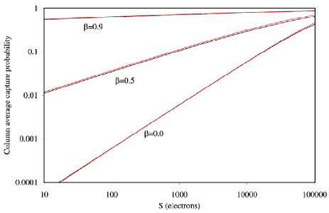
Figure 4: Column-average electron capture probability, $\bar{P_{c}}(S)$, according to equation 15 (black) and the simple approximation given in equation 18 (red). Note that a rather small value of capture cross-section ($3\times 10^{-18}$ cm²) has been used in this example to illustrate the dependence over a large signal range. Note that the difference is smaller for larger values of the capture cross section where the curve would be almost flat and close to unity.

Figure 4 illustrates equation 15 (black) and the simple approximation given in equation 18 (red). The agreement is certainly good enough to justify the use of the simpler expression. Hence, we may combine equations 5 and 18 to give an expression for the number of electrons, $N_{c}$, that will be captured by a given trap species during the transit of an integrating signal packet, $S$, as a function of physical trap parameters and the initial trap occupancy, $N_{o}$:

$$N_{c}=\frac{\gamma S^{\beta}-N_{o}}{\gamma S^{\beta-1}+1}\left(1-\exp\left\{-\alpha\left(\frac{S}{2}\right)^{1-\beta}\right\}\right)$$ (19)

Note that equation 19 can give negative trapping when the number of occupied traps exceeds the number of interacting electrons and vacant traps. If the de-trapping process were the reverse of the trapping process, then this could be used directly to model trapping and de-trapping. However, trapping and de-trapping time constants are very different so this is not the case. When implementing equation 19, it is therefore necessary to avoid negative trapping. Thus, in summary, we have a model for electron capture by one trap species in TDI mode:

$$N_{c}=\mbox{MAX}\left[\frac{\gamma S^{\beta}-N_{o}}{\gamma S^{\beta-1}+1}\left(1-\exp\left\{-\alpha\left(\frac{S}{2}\right)^{1-\beta}\right\}\right)\>,\>0\right]$$ (20)

$$\mbox{where}\qquad\gamma=\frac{2n_{t}V_{g}x}{\left(1+\beta\right)FWC^{\beta}}\qquad\mbox{and}\qquad\alpha=\frac{t\sigma v_{t}FWC^{\beta}}{2V_{g}}$$ (21)

3.2 Electron trapping in imaging mode (non-TDI)

There are several circumstances where it is necessary to model trapping in non-TDI mode. These include the treatment of charge-injection lines which are injected at the top of the CCD and do not integrate along the CCD, modelling transfer along the serial register and of course applying the model to other missions which are not operating in TDI mode at all.

There are only a couple of differences in the final equations related to the fact that the signal is not integrating during the transfer. In imaging mode, the model may be summarised:

$$N_{c}=\mbox{MAX}\left[\frac{\gamma S^{\beta}-N_{o}}{\gamma S^{\beta-1}+1}\left(1-\exp\left\{-\alpha S^{1-\beta}\right\}\right)\>,\>0\right]$$ (22)

$$\mbox{where}\qquad\gamma=\frac{2n_{t}V_{g}}{FWC^{\beta}}\left(x+i\right)\qquad\mbox{and}\qquad\alpha=\frac{t\sigma v_{t}FWC^{\beta}}{2V_{g}}$$ (23)

where $x$ indicates the position on the CCD (in pixels) of the image to be processed, i.e., small $x$ for an image close to the readout node and large $x$ for objects far from the readout node and $i$ is the pixel coordinate of each sample within the image to be processed.

3.3 Electron release

If we assume that every occupied trap in the column has a time equal to one TDI period ($t$) in which to release the captured electron into a given sample, then the probability, $P_{r}$, that the trap will release the electron into the sample is simply:

$$P_{r}=1-\mbox{e}^{-\frac{t}{\tau_{r}}}$$ (24)

where $\tau_{r}$ is the trap release time constant. The number of electrons released into the sample during a transit along the column is then simply:

$$N_{r}=N_{o}\left\{1-\mbox{e}^{-\frac{t}{\tau_{r}}}\right\}$$ (25)

3.4 Column state parameter and initial state

In implementing any CCD trapping model, it is very important to consider the state or occupancy of the traps (the value of $N_{o}$) at the beginning of the simulation. In the event that a continuous, unbroken stream of realistic data (including background etc.) were to be simulated (much longer than the capture or release time constants of the slowest traps), it would be sufficient to start with all traps empty or all traps full and to disregard the first few minutes of simulated data rather than to explicitly initialize $N_{o}$ with a realistic value. However, this is rarely practical, the state of the slower traps prior to the transit of a source will be dominated by two main factors. These are the time since the last charge injection and the level of constant or slowly varying optical background (some fraction of slow traps kept full). We may therefore treat these two dependencies explicitly in order to quickly determine the state of traps prior to the transit of an astronomical source (or test data image).

3.4.1 Diffuse optical background

The effect of a constant (or slowly varying) low-level optical background upon the occupancy of slow traps has been demonstrated during the Gaia radiation test campaigns (see Section 2). This reveals information about the temporal dependency or dynamics of trapping since the exposure time of traps to a constant background is radically different from the exposure time to transient sources. It also reveals something about the confinement volume of electrons within pixels since low levels of background appear capable of filling entire trap species.

Considering TDI mode for Gaia, the initial trap occupancy, $N_{o}|_{init}$ due to a constant optical background is determined as follows. It is assumed that in the continuous presence of background electrons, traps will reach an equilibrium state of occupancy when $N_{c}=N_{r}$. Thus:

$$\frac{\gamma S_{dob}^{\beta}-N_{o}|_{init}}{\gamma S_{dob}^{\beta-1}+1}\left(1-\exp\left\{-\alpha\left(\frac{S_{dob}}{2}\right)^{1-\beta}\right\}\right)$$

$$=N_{o}|_{init}\left\{1-\mbox{e}^{-\frac{t}{\tau_{r}}}\right\}$$ (26)

where $S_{dob}$ is the diffuse optical background level in electrons per pixel measured at the readout register.

Solving equation 26 for $N_{o}|_{init}$ gives:

$$N_{o}|_{init}=\frac{AB}{A+C}$$ (27)

where:

$$A=\frac{1-\exp\left\{-\alpha\left(\frac{S_{dob}}{2}\right)^{1-\beta}\right\}}{\gamma S_{dob}^{\beta-1}+1}\qquad\qquad\text{and}$$

$$B=\gamma S_{dob}^{\beta}\qquad\qquad\text{and}$$

$$C=1-\mbox{e}^{-\frac{t}{\tau_{r}}}$$ (28)

3.4.2 Time since charge injection

In the case of a high level of charge injection it may be sufficient to assume that the injection fills all traps which then subsequently empty at a rate determined by the exponential trap release time constant until they reach the occupancy level determined by the diffuse optical background. For example, adding an exponential term to equation 27, the initial state of the column would be given by:

$$N_{o}|_{init}=2n_{t}V_{g}x\mbox{e}^{-\frac{t_{ci}}{\tau_{r}}}+\frac{AB}{A+C}\left(1-\mbox{e}^{-\frac{t_{ci}}{\tau_{r}}}\right)$$ (29)

where $t_{ci}$ is the time elapsed since charge injection and $\tau_{r}$ is the trap release time constant.

However, in the case of lower levels of charge injection where it may not be adequate to assume that all traps are saturated, it is better to simulate the capture of electrons from the charge injection lines explicitly to determine the fraction of traps that are filled. These then empty according to the exponential trap release time constant as before. In order to simulate charge injection correctly, it is necessary to consider that charge injection is effectively in image mode rather than TDI mode.

4 Examples of Modelling Results

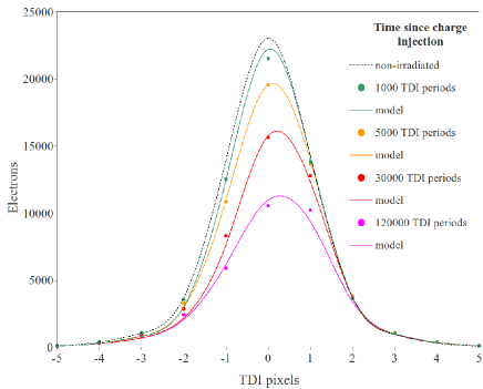
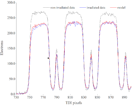
Figure 5: Left: Representive fits to Gaia test data for Gaia magnitude $\sim$15 point sources with varying time since charge injection. The non-irradiated curve is derived from data acquired on a section of a CCD which has not undergone radiation damage. The other curves are derived from data acquired from a radiation-damaged section of the same detector, with a uniform damage level throughout this section. Right: Similarly, a section of Gaia dispersed test data for Gaia magnitude $\sim$10 and with a diffuse optical background of 0.77 $\,\mathrm{e^{-}pix^{-1}s^{-1}}$ . These data are representative of what will be observed with the Radial Velocity Spectrometer (RVS) instrument onboard Gaia. For the fits shown in both plots model parameters are derived using a global fit to all test data from magnitude 13.25 to magnitude 20 and with delays since prior charge-injections from 30 ms to 120 s. Note that readout direction is to the left for both plots.

It is beyond the scope of this work to provide a detailed analysis of the application of the model to Gaia test data. Instead, we provide a limited graphical indication that the model is qualitatively capable of reproducing trapping effects observed in test data.

Figure 5 (left panel) indicates the distortion observed in the parallel direction in Gaia test data as a function of time since charge injection. The datapoints are measured data and the solid lines are CDM model results. Note that a single set of trap parameter values was used to generate all of these model curves. Figure 5 (right panel) shows the fit of the model to radiation damaged dispersed spectral data (similar to what will be observed with the Radial Velocity Spectrometer (RVS) instrument onboard Gaia). Curves are shown for data taken on non-irradiated and irradiated sections of a CCD, with the output of the CDM also over-plotted. Again, a single set of model parameters has been selected giving a reasonable fit to all data. The CDM has also been used to examine the effects of radiation damage on CTI in Euclid (e.g., see Laureijs et al., 2012; Cropper et al., 2013) CCDs.

5 Conclusions

The ESA astrometric mission Gaia, scheduled for launch in 2013, will be subject to a systematic bias in its measurements due to radiation damage-induced CTI in its CCD detectors. In order to sufficiently calibrate out this bias it is planned to forward model the charge distortion to the CCD images at the CCD sample level. The use of an analytical charge distortion model, which must be computationally inexpensive, is fundamental to Gaia reaching its scientific goals. It treats electron trapping and de-trapping within each CCD column (and serial register) in a single step ensuring that it is computationally fast, although still based on physical theory. A description of the model is presented, and its ability to qualitatively reproduce the CTI effects in Gaia test data is demonstrated. The model can be applied to CCDs operating in both TDI and imaging mode and hence is fully general.

References

- Brown & van Leeuwen (2008) Brown S., van Leeuwen F., 2008, Analysis of the CCN10 data set. CTI effects on a Gaia astrometric CCD [An internal Technical Note]
- Cropper et al. (2013) Cropper M., Hoekstra H., Kitching T., Amiaux J., Massey R., Miller L., Mellier Y., Rhodes J., Rowe B., Pires S., Saxton C., Scaramella R., MNRAS, submitted
- de Bruijne et al. (2010) de Bruijne J., Kohley R., Prusti T., 2010, in Society of Photo-Optical Instrumentation Engineers (SPIE) Conference Series Vol. 7731, Gaia: 1,000 million stars with 100 CCD detectors
- de Bruijne (2012) de Bruijne J. H. J., 2012, APSS, 341, 31
- Hardy et al. (1998) Hardy T., Murowinski R., Deen M. J., 1998, IEEE Transactions on Nuclear Science, 45, 154
- Holl et al. (2012) Holl B., Prod’homme T., Lindegren L., Brown A. G. A., 2012, MNRAS, 422, 2786
- Janesick (2001) Janesick J. R., 2001, Scientific charge-coupled devices
- Laureijs et al. (2012) Laureijs R., Gondoin, P., Duvet, L., Saavedra Criado, G., Hoar, J. et al., 2012, in Society of Photo-Optical Instrumentation Engineers (SPIE) Conference Series Vol. 8442, Euclid: ESA’s mission to map the geometry of the dark universe
- Lindegren (2008) Lindegren L., 2008, Modelling radiation damage effects for Gaia - A first-order Charge Distortion Model (CDM-01) [An internal Technical Note]
- Lindegren et al. (2008) Lindegren L., Babusiaux C., Bailer-Jones C., Bastian U., Brown A. G. A., Cropper M., Høg E., Jordi C., Katz D., van Leeuwen F., Luri X., Mignard F., de Bruijne J. H. J., Prusti T., 2008, in W. J. Jin, I. Platais, & M. A. C. Perryman ed., IAU Symposium Vol. 248 of IAU Symposium, The Gaia mission: science, organization and present status. pp 217–223
- Lindegren et al. (2012) Lindegren L., Lammers U., Hobbs D., O’Mullane W., Bastian U., Hernández J., 2012, A&A, 538, A78
- Perryman et al. (2001) Perryman M. A. C., de Boer K. S., Gilmore G., Høg E., Lattanzi M. G., Lindegren L., Luri X., Mignard F., Pace O., de Zeeuw P. T., 2001, A&A , 369, 339
- Prod’homme et al. (2011) Prod’homme T., Brown A. G. A., Lindegren L., Short A. D. T., Brown S. W., 2011, MNRAS, 414, 2215
- Seabroke et al. (2013) Seabroke G. M., Prod’homme T., Murray N. J., Crowley C., Hopkinson G., Brown A. G. A., Kohley R., Holland A., MNRAS, submitted
- Short (2006) Short A., 2006, Independent analysis of EADS Astrium CCN10 radiation test data [An internal Technical Note]