Shock creation and Painlevé property of colliding peakons in the Degasperis-Procesi Equation

Abstract

The Degasperis-Procesi equation (DP) is one of several equations known to model important nonlinear effects such as wave breaking and shock creation. It is, however, a special property of the DP equation that these two effects can be studied in an explicit way with the help of the multipeakon ansatz. In essence this ansatz allows one to model wave breaking as a collision of hypothetical particles (peakons and antipeakons), called henceforth collectively multipeakons. It is shown that DP multipeakons have Painlevé property which implies a universal wave breaking behaviour, that multipeakons can collide only in pairs, and that there are no multiple collisions other than, possibly simultaneous, collisions of peakon-antipeakon pairs at different locations. Moreover, it is demonstrated that each peakon-antipeakon collision results in creation of a shock thus making possible a multi shock phenomenon.

1 Introduction

The Degasperis-Procesi (DP) equation [9]

$$u_{t}-u_{txx}+4uu_{x}=3u_{x}u_{xx}+uu_{xxx}$$ (1.1)

belongs to a class of one-dimensional wave equations which have attracted considerable attention over the last decade, following the most studied equation in this class, namely, the Camassa-Holm (CH) equation [3]

$$u_{t}-u_{txx}+3uu_{x}=2u_{x}u_{xx}+uu_{xxx}.$$

Both these equations can be derived from the governing equations under the assumption of moderate amplitude [13, 7]. What makes them special is that, on one hand, both are Lax integrable, on the other, both exhibit wave breaking phenomenon not captured by linear theory or shallow water, small amplitude theory like the Korteweg-deVries equation. The most relevant to this paper study of the breakdown of solutions for the CH equation was done by H.P. McKean [22, 21]. In these works, it was argued that the breakdown of the CH waves is controlled by a kind of caricature of the higher dimensional vorticity, namely, $m=u-u_{xx}$ (see [20] ). In particular, it is the initial relative position of regions with positive $m$ versus negative $m$ that signals whether the breakdown will happen at some later, finite, time. One of the fascinating aspects of both the CH and DP equations is the existence of special solutions, peakons, which play the role of basic building blocks of the underlying full theory. Peakons are a simple superposition of exponential terms

$$u(x,t)=\sum_{j=1}^{n}m_{j}(t)e^{-|x-x_{j}(t)|}$$

for which the function $m$ referred to earlier is $m=2\sum_{j=1}^{n}m_{j}\delta_{x_{j}}$. Were we to take the analogy with vorticity at its face value, $m$ for peakons could be viewed as a collection of point vortices, situated at $x_{j}(t)$s, of strength $m_{j}(t)$ each, initially ordered in some fixed way, say, $x_{1}(0)<x_{2}(0)<\cdots<x_{n}(0)$. The case of CH peakons shows that if the strengths $\{m_{k}(0):1\leq k\leq n\}$ are not of the same sign then collisions can occur, meaning that $x_{j}(t_{c})=x_{j+1}(t_{c})$ for some $j$ and some time $t_{c}$. Each collision is accompanied by a blow-up of $m_{j}(t_{c})$ and $m_{j+1}(t_{c})$ resulting in the derivative $u_{x}(t_{c})$ becoming unbounded even though $u(t_{c})$ remains bounded, in fact continuous. Thus peakons can be used to test ideas about wave breaking, the advantage being that the peakon dynamics is described by a finite system of ODEs (see Section 2 ). The analysis of the CH peakon collisions in this case was done in [1] with the help of explicit formulas. In short, the CH peakon problem can be solved by Stieltjes’ formulas involving continued fractions [2]. Moreover, the underlying boundary value problem is self-adjoint, in fact it is equivalent to an inhomogeneous string which remains isospectral under the CH flow.

The case of the DP equation is superficially similar to the CH case. However, deeper analysis shows a remarkable number of new features. For example, the associated spectral problem, termed a cubic string in [19], is not self-adjoint and this has the immediate consequence that the inverse problem is by far more involved. The peakon problem in the case of the positive measure, that is when all weights $m_{j}$s are positive, was solved explicitly in [19]. However, the generalization to the case of a signed measure $m$ is not straightforward since the spectral data breaks up into several types depending on the degeneracy of the spectrum, as well as on certain coincidental phenomena of anti-resonances (eigenvalues $z_{i},z_{j}$ pairing according to $z_{i}+z_{j}=0$). By contrast, the distinction between peakons for positive measure $m$ and peakons for the signed measure $m$ is less sharp for the CH case where the formulas for peakons can be analytically continued from former to latter. This is not so for the DP case. This difficulty notwithstanding, in a way analogous to what happens in the CH case, the presence of a collision signals an occurrence of wave breaking; in the DP context the connection between wave breaking and peakon collisions was studied earlier by H. Lundmark in [17] for the case $n=2$ and further by the present authors in [23] for $n=3$. Important questions of stability and general analytic results dealing with DP peakons and the DP wave breaking have been addressed in [15, 14, 16, 10]. A considerable amount of work has been also done on adapting numerical schemes to deal with the DP equation; we just mention a few: an operator splitting method of Feng and Liu [11], or numerical schemes discussed by Coclite, Karlsen and Risebro in [6].

The DP equation, in contrast to the CH equation, admits shock solutions (see [4, 5] for a general, very thorough, discussion). It was H. Lundmark who introduced the concept of shockpeakons

$$u(x,t)=\sum_{j=1}^{n}\{m_{j}(t)-s_{j}(t)\operatorname{sgn}(x-x_{j}(t))\}e^{-|x-x_{j}(t)|},$$

for which

$$m=2\sum_{j=1}^{n}\{m_{j}\delta_{x_{j}}+s_{j}\delta_{x_{j}}^{\prime}\},$$ (1.2)

and showed that the solution describing a collision of two peakons has a unique entropy extension to shockpeakons. He also hypothesized that this might be a general phenomenon valid also for $n>2$. We prove his conjecture. More precisely we prove that the distributional limit of $m$ at the collision point $t_{c}$ indeed produces shockpeakon data (1.2) with positive shock strengths $s_{j}$ thus allowing a unique entropy weak extension (see Theorem 5.1 and Corollary 5.2).

Let us briefly describe our strategy. Instead of analyzing numerous spectral types we concentrate on analytic properties of $x_{j}(t),m_{j}(t)$ as functions of $t$. To this end we analyze the inverse spectral problem for the cubic string with the input data of a finite, signed measure. We prove that each $x_{j}(t)$ must be a holomorphic function at $t_{c}$, while $m_{j}(t)$ is in general only meromorphic (Theorem 3.5). Then we perform singularity analysis of the ODEs describing peakons (2.6) and prove their Painlevé property with the help of Theorems 3.5 and 3.6 followed by a singularity analysis at the time of collisions described by Theorem 4.5.

The plan of the paper is as follows: we review basic facts about the DP equation in Section 2, in Section 3 we discuss the inverse problem for peakons of both signs generalizing the uniqueness result known from the pure peakon case [19] and use this result to establish analytic properties of positions $x_{j}$s and masses $m_{j}$s. In Section 4 we analyze the singular behaviour at the time of collisions and establish a universal singularity pattern according to which, in the leading term, only the time of the blowup depends on the initial conditions not the residue. This fact is proven in Theorem 4.5. We furthermore rule out triple collisions in Theorem 4.7, and give an example of a simultaneous collision, in different positions, of two peakon-antipeakon pairs; finally in Section 5 we prove Theorem 5.1 stating that the distributional limit of colliding peakons is indeed a shockpeakon.

2 Basic Facts about the DP equation

The nonlinear equation

$$u_{t}-u_{xxt}+4uu_{x}=3u_{x}u_{xx}+uu_{xxx},$$ (2.1)

often written as

$$m_{t}+m_{x}u+3mu_{x}=0,\qquad m=u-u_{xx},$$ (2.2)

was introduced by Degasperis and Procesi [9] as an example of a nonlinear partial differential equation satisfying asymptotic integrability appearing in the family of third order dispersive equations:

$$u_{t}-\alpha^{2}u_{xxt}+\gamma u_{xxx}+c_{0}u_{x}=(c_{1}u^{2}+c_{2}u_{x}^{2}+c_{3}uu_{xx})_{x},$$

other examples of integrable equations in this family are the Korteweg-deVries equation (KdV) and the Camassa-Holm (CH) equation. Formal integrability for the DP equation was established by Degasperis, Holm and Hone [8] through the construction of a Lax pair and a bi-Hamiltonian structure. In particular, it was shown in [8] that the DP equation admits the Lax pair:

$$(\partial_{x}-\partial_{xxx})\Psi=zm\Psi,\qquad\Psi_{t}=[z^{-1}(1-\partial^{2}_{x})+u_{x}-u\partial_{x}]\Psi.$$ (2.3)

Moreover, one can impose additional boundary conditions provided they do not violate the compatibility of these equations. One such a pair of boundary conditions was introduced in [19]:

$$\Psi\rightarrow e^{x},\text{ as }x\rightarrow-\infty,\qquad\Psi\text{ is bounded as }x\rightarrow+\infty,$$ (2.4)

where it was also shown that the spectrum of this boundary value problem will remain time invariant (isospectral deformation). It suffices for our purposes to restrict our attention to the case in which $m$ is a finite discrete (signed) measure. Thus for the remainder of the paper we will use the multipeakon ansatz

$$u(x,t)=\sum_{i=1}^{n}m_{i}(t)\,e^{-|x-x_{i}(t)|}$$ (2.5)

where $x_{1}(0)<x_{2}(0)<\cdots<x_{n}(0)$ and $m_{i}(0)$ can have both positive and negative values. This ansatz produces $m=2\sum_{i=1}^{n}m_{i}\delta_{x_{i}}$. Moreover, with the proper interpretation of weak solutions to equation (2.1) we can easily check that $u$ is a weak solution to (2.1) provided $x_{i}(t),m_{i}(t)$ satisfy the following ODEs

$$\dot{x}_{k}(t)=u(x_{k})=\sum_{i=1}^{n}m_{i}(t)\,e^{-|x_{k}(t)-x_{i}(t)|},\qquad$$ (2.6a)

$$\dot{m}_{k}(t)=2\,m_{k}(t)\,\bigl{\langle}u_{x}(x_{k})\bigr{\rangle}=2\,m_{k}(t)\sum_{i=1}^{n}m_{i}(t)\operatorname{sgn}(x_{k}(t)-x_{i}(t))\,e^{-|x_{k}(t)-x_{i}(t)|},$$ (2.6b)

where $\bigl{\langle}f(x)\bigr{\rangle}=\lim_{\epsilon\to 0^{+}}\frac{1}{2}[f(x+\epsilon)+f(x-\epsilon)]$ is the average of $f$ at the point $x$. We will refer to $m_{j}$s as masses to emphasize their role in the spectral problem. We also need a bit of terminology regarding the phenomenon of breaking. We will say that a collision occurred at some time $t_{c}$ if $x_{i}(t_{c})=x_{i+1}(t_{c})$ for some $i$. We can make this concept more geometric by introducing a configuration space in which to study peakon solutions, namely the sector $X=\{{\bf x}\in\mathbf{R}^{n}\ |x_{1}<x_{2}<\cdots<x_{n}\}$. Then a collision corresponds to the solution $x_{i}$ hitting the boundary of $X$.

A very useful property of equations (2.6) is the existence of $n$ constants of motion. This follows readily from Theorem 2.10 in [19].

Lemma 2.1.

$M_{p}\,(1\leq p\leq n)$, given by:

$$M_{p}=\sum_{I\in{[1,k]}\choose p}\left(\prod_{i\in I}m_{i}\right)\left(\prod_{j=1}^{p-1}(1-e^{x_{i_{j}}-x_{i_{j+1}}})^{2}\right)$$

are $n$ constants of motion of the system of equations (2.6), where $\binom{[1,n]}{p}$ is the set of all $p$-element subsets $I=\left\{i_{1}<\dots<i_{p}\right\}$ of $\left\{1,\dots,n\right\}$.

3 Inverse Problem for multipeakons

The boundary value value problem (2.3) and (2.4) can be transformed to a finite interval boundary value problem, the cubic string problem. Indeed, following [19], the change of variables (Liouville transformation)

$$y=\tanh\frac{x}{2},\qquad\Psi(x)=\frac{2\phi(y)}{1-y^{2}}$$ (3.1)

maps the DP spectral problem into the cubic string problem:

$$-\phi_{yyy}(y) =zg(y)\phi(y),\qquad-1<y<1,$$ (3.2a)

$$\phi(-1) =\phi_{y}(-1)=\phi(1)=0,$$ (3.2b)

where $g$ is the transformation of the measure $m$ induced by the Liouville transformation (3.1). Furthermore, as one can explicitly check, $g$ is also a finite signed measure and its support does not include the endpoints if the original measure $m$ is a finite signed measure. More concretely, in this paper,

$$g=\sum_{i=1}^{n}g_{i}\delta_{y_{i}},\quad-1<y_{1}<y_{2}<\dots<y_{n}<1,$$ (3.3)

with weights $g_{i}\in\mathbf{R}$. The inverse problem is studied with the help of two Weyl functions.

Definition 3.1.

Let $\phi(y;z)$ denote the solution to the initial value problem (3.2a) with initial conditions $\phi(-1;z)=\phi_{y}(-1;z)=0,\,\phi_{yy}(-1;z)=1$. The Weyl functions are ratios:

$$W(z)=\frac{\phi_{y}(1;z)}{\phi(1;z)},\qquad Z(z)=\frac{\phi_{yy}(1;z)}{\phi(1;z)}.$$

These two functions encode spectral information needed to solve the inverse problem. It is easy to verify that in the case of (3.3) both $W(z)$ and $Z(z)$ are rational functions which makes inversion algebraic. However, in contrast to the pure peakon case $g_{i}>0$, the spectrum of the boundary value problem (3.2a) is in general complex and not necessarily simple. This makes the inversion more challenging. Regardless of the complexity of the spectrum though the Weyl functions undergo a simple evolution under the DP flow. Indeed, using the second member of the Lax pair given by (2.3) one can find the time evolution of $W(z)$ and $Z(z)$. To wit, using results from Theorem 2.3 in [23] we obtain the following characterization of the time evolution of $W(z)$ and $Z(z)$.

Theorem 3.2.

Let

$$\frac{W(z)}{z}=\sum_{j}\sum_{k=1}^{d_{j}}\frac{b_{j}^{(k)}}{(z-\lambda_{j})^{k}}+\frac{1}{z},$$

be the partial fraction decomposition of $\frac{W(z)}{z}$, where $d_{j}$ denotes the algebraic degeneracy of the $j$-th eigenvalue. Then the DP time evolution implies:

1. $$b^{(k)}_{j}=p^{(k)}_{j}(t)e^{\frac{t}{\lambda_{j}}},$$

   where $p^{(k)}_{j}(t)$ is a polynomial in $t$ of degree $d_{j}-k$.

2. $M_{+}\stackrel{{\scriptstyle\rm{def}}}{{=}}\sum_{k=1}^{n}m_{k}e^{x_{k}}=\sum_{j}\dot{b}^{(1)}_{j}$.

3. $$\dot{W}=\frac{W-1}{z}+M_{+},\quad\dot{Z}=(W-1)M_{+}+\dot{W}$$

We immediately have:

Corollary 3.3.

Under the DP flow the Weyl functions $W,Z$ are entire functions of time.

The uniqueness result below plays a major role in the solution to the inverse problem.

Theorem 3.4.

Suppose $\Phi:g\rightarrow\{W(z),Z(z)\}$ is the map that associates to the cubic string problem (3.2) with a finite signed measure $g$, the Weyl functions $W(z),Z(z)$. Then $\Phi$ is injective.

Proof.

The proof relies on remarks made in [18]. We will construct a recursive scheme to solve the inverse spectral problem; given $W$ and $Z$ obtained from the map $\Phi$ we will reconstruct the finite, signed measure $g$ whose Weyl functions are $W$ and $Z$. More precisely, we will show that the $y_{j}$’s and $g_{j}$’s in equation (3.3) are uniquely determined from $W(z),Z(z)$. First we recall that $W$ and $Z$ are constructed from solutions to the initial value problem (see Definition 3.1)

$$-\phi_{yyy}(y) =zg(y)\phi(y),\qquad-1<y<1,$$ (3.4a)

$$\phi(-1) =\phi_{y}(-1)=0,\quad\phi_{yy}(-1)=1$$ (3.4b)

Masses $g_{j}$ are situated at $y_{j},\,1\leq j\leq n$ and for convenience let us set $y_{0}=0,\,y_{n+1}=1$ and denote by $l_{j}=y_{j+1}-y_{j}$ the length of the interval $(y_{j},y_{j+1})$. Then on each interval $(y_{j},y_{j+1})$ the solution to (3.4) takes the form

$$\phi(y)=\phi(y_{j+1})+\phi_{y}(y_{j+1})\,(y-y_{j+1})+\phi_{yy}(y_{j+1}-)\,(y-y_{j+1})^{2}/2,\quad 0\leq j\leq n$$

and the condition of crossing $y_{j+1}$ is: continuity of $\phi$ and $\phi_{y}$ and the jump condition $\phi_{yy}(y_{j+1}+)-\phi_{yy}(y_{j+1}-)=-zg_{j+1}\phi(y_{j+1})$. We establish, for example by an easy induction,

$$\left(\phi(y_{j+1}),\phi_{y}(y_{j+1}),\phi_{yy}(y_{j+1}-)\right)=(-z)^{j}\prod_{k=1}^{j}\frac{g_{k}l^{2}_{k-1}}{2}\,\left(l^{2}_{j}/2,l_{j},1\right)+O(z^{j-1}),$$ (3.5)

valid for $0\leq j\leq n$, with the convention that for $j=0$ the product equals $1$ and there is no remainder. Likewise,

$$\left(\phi(y_{j}),\phi_{y}(y_{j}),\phi_{yy}(y_{j}+)\right)=(-z)^{j}\prod_{k=1}^{j}\frac{g_{k}l^{2}_{k-1}}{2}\,\left(0,0,1\right)+O(z^{j-1}),$$ (3.6)

valid for $1\leq j\leq n$.

For $0\leq j\leq n$ we define $(w_{2j},z_{2j})=(\frac{\phi_{y}}{\phi},\frac{\phi_{yy}}{\phi})|_{y=y_{j+1}-}$ and $(w_{2j-1},z_{2j-1})=(\frac{\phi_{y}}{\phi_{yy}},\frac{\phi}{\phi_{yy}})|_{y=y_{j}+}$. These quantities are essentially the left hand and the right hand analogs of Weyl functions introduced in Definition 3.1 and correspond to shorter strings terminating at $y_{j+1}$ with no mass at the endpoint, or terminating at $y_{j}$ but with the mass $g_{j}$ at the end. Equation (3.4) implies that the sequence $(w_{2j},z_{2j},w_{2j-1},z_{2j-1})$ satisfies the recurrence relations

$$w_{2j-1}=\frac{w_{2j}}{z_{2j}}-l_{j},\qquad z_{2j-1}=\frac{1}{z_{2j}}-l_{j}\frac{w_{2j}}{z_{2j}}+\frac{l_{j}^{2}}{2},$$ (3.7)

$$w_{2j-2}=\frac{w_{2j-1}}{z_{2j-1}},\qquad z_{2j-2}=\frac{1}{z_{2j-1}}+zg_{j};$$ (3.8)

the iteration starts at $w_{2n}=W(z),z_{2n}=Z(z)$ and terminates at $w_{-1},z_{-1}$. Moreover, based on equations (3.5) and (3.6), we easily establish

$$w_{2j}=\frac{2}{l_{j}}+O(\frac{1}{z}),\quad z_{2j}=\frac{2}{l_{j}^{2}}+O(\frac{1}{z}),\quad w_{2j-1}=z_{2j-1}=O(\frac{1}{z}),\quad\text{as }z\rightarrow\infty,$$ (3.9)

which implies that the quantities $\{l_{j},g_{j}\}$ are determined in each step from the large $z$ asymptotics of terms known from the previous step. Indeed, if we denote by $a^{(m)}$ the coefficient of $z^{-m}$ in the expansion of a holomorphic function $a(z)$ at $z=\infty$ we obtain the recovery formulas

$$l_{j}=\frac{2}{w_{2j}^{(0)}},\qquad g_{j}=-\frac{1}{z_{2j-1}^{(1)}}.$$ (3.10)

Thus we proved that given a pair of Weyl functions $W(z),Z(z)$ obtained from a cubic string problem (3.4) with a finite, signed measure $g$, there exists a unique solution to the recurrence relations (3.7) subject to (3.9) and thus a unique cubic string corresponding to $W(z),Z(z)$. ∎

We are now ready to state the central theorem of this section

Theorem 3.5.

Let $\{x_{j}(t),m_{j}(t)\},j=1,\dots,n$ be the positions and masses of the peakon ansatz (2.5) corresponding to an arbitrary signed measure $m=2\sum_{j=1}^{n}m_{j}\delta_{x_{j}}$, satisfying peakon equations (2.6) on the time interval $(0,t_{c})$ and suppose that a collision occurs at $t_{c}$. Then the positions $x_{1}(t)\dots,x_{n}(t)$ are analytic functions at $t_{c}$, while the masses $m_{1}(t)\dots m_{n}(t)$ are given by meromorphic functions at $t_{c}$.

Proof.

Given the initial conditions $\{x_{1}(0)<x_{2}(0)<\dots<x_{n}(0)\}$ and
$\{m_{1}(0),m_{2}(0),\dots,m_{n}(0)\}$ we set up the string problem (3.2a) after mapping $m(0)$ to $g(0)$. This produces the Weyl functions $W(0),Z(0)$, which under the peakon flow evolve as entire functions of time in view of Corollary 3.3. We then set up the recursive scheme (3.7) with $W(t),Z(t)$ as inputs. At each stage of recursion only rational operations are involved and since the recursion is finite the formulas (3.10) result in functions meromorphic in $t$. Thus all $g_{j},y_{j}$ are meromorphic in $t$. For $t<t_{c}$ all distances $l_{j}>0$ and at $t_{c}$ some $l_{i}$ vanishes but all $l_{j}$ remain finite, because this is a finite string. Hence $l_{j}(t)$ is regular at $t_{c}$ hence analytic there. For a signed measure $g$ there are no bounds restrictions on individual $g_{j}$ so in general $g_{j}$ remains meromorphic at $t_{c}$. Mapping back to the real axis is afforded by $y=\tanh\frac{x}{2}$; hence positions of individual masses are given by $x_{j}=\ln\frac{y_{j}+1}{y_{j}-1}$. The only singular points of this map are for $y_{j}=\pm 1$ which means the end of the string or, after mapping the problem back to the real axis, $\pm\infty$. However, based on results in [23], none of the masses can escape to $\pm\infty$ in finite time. So $\frac{y_{j}+1}{y_{j}-1}$ is in the domain of analyticity of $\ln$ and hence the $x_{j}$s are analytic at $t_{c}$. The relation between the measures $m$ and $g$ appearing in equations (2.3) and (3.2a) is given by $m_{j}=\frac{(1-y_{j}^{2})^{2}}{8}g_{j}$ which implies the claim since $g_{j}$ is meromorphic and $y_{j}$ analytic. ∎

The above theorem establishes that the only singular points of solutions to the peakon ODE system (2.6a) and (2.6b) are poles. Since the inverse problem argument is valid for a fixed ordering $x_{1}<x_{2}<\cdots<x_{n}$ of masses, the analytic continuation of masses and positions into the complex domain in $t$ will satisfy equations (2.6a) and (2.6b) in which $\operatorname{sgn}(x_{k}-x_{i}),e^{-\left\lvert(x_{k}-x_{i})\right\rvert}$ are replaced with $\operatorname{sgn}(k-i)$, $e^{-\operatorname{sgn}(k-i)(x_{k}-x_{i})}$ respectively, to be consistent with the original ordering. It is for these equations that we note the absence of movable critical points also known as Painlevé property [12]. To facilitate the statement of the last theorem of this section we set $X_{i}=e^{x_{i}},\,1\leq i\leq n$ and rewrite the system (2.6a) and (2.6b) in new variables $\{m_{i},X_{i}\}$.

Theorem 3.6 (Painlevé property).

The system of differential equations

$$\dot{X}_{k}=X_{k}\sum_{i=1}^{n}m_{i}\,\left(\frac{X_{i}}{X_{k}}\right)^{\operatorname{sgn}(k-i)},\,\quad\dot{m}_{k}=2\,m_{k}\sum_{i=1}^{n}m_{i}\operatorname{sgn}(k-i)\,\left(\frac{X_{i}}{X_{k}}\right)^{\operatorname{sgn}(k-i)}$$

has the Painlevé property.

Proof.

First we observe (using the variables of the proof of Theorem 3.5) that $X_{i}=\frac{y_{i}+1}{y_{i}-1}$, hence $X_{i}$s are meromorphic in $t$ because so are $y_{i}$s. The formulas for $X_{i}$s and $m_{i}$s obtained from the inverse problem are meromorphic in $t$ in the complex plane $\mathbf{C}$ and depend on $2n$ constants (spectral data consisting, in the generic case, of $n$ positions of poles and $n$ residues of the Weyl function $W$), which for the cubic string problem, in view of the ordering condition, are confined to an open set in $\mathbf{C}^{2n}$ by continuity of the inverse spectral map. Relaxing that condition results in a solution depending on $2n$ arbitrary constants which comprises a general solution which is meromorphic in $t$ in the whole complex plane $\mathbf{C}$. ∎

In the remainder of the paper we will concentrate on the specific singularity structure at the time of collisions of peakons.

4 Blow-up behaviour

We now proceed to establish several theorems on peakon collisions for DP equation. To begin with we recall the definition of a peakon collision briefly discussed in the introduction. We call $t_{c}$ the collision time if there exists some $i$ such that

$$\lim_{t\to t_{c}^{-}}x_{i}(t)=\lim_{t\to t_{c}^{-}}x_{i+1}(t),$$ (4.1)

where $x_{i}(t)$s are the position functions in the ansatz (2.5). Equivalently, we say that the $i$-th peakon collides with the $(i+1)$-th peakon at the time $t_{c}$. If there exist more than two position functions being identical at $t_{c}$ then we will say that a multiple collision happens at $t_{c}$.

In this section, we describe the behaviour of the peakon dynamical system (2.6) in the neighbourhood of a collision time $t_{c}$.

To this end we need to study a special skew-symmetric $n\times n$ real matrix $A_{n}$ given by

$$A_{n}=\left[\operatorname{sgn}(i-j)a_{ij}\right]$$ (4.2)

whose entries satisfy $a_{ij}=a_{ji}$ and

$$a_{ij}=a_{il}a_{lj}\neq 0,\quad\text{for all $0<i<l<j<n$.}$$ (4.3)

The following propositions hold for such a matrix.

Lemma 4.1.

There exists a matrix $P$ with $\det P=1$ such that $P^{T}A_{n}P=B_{n}$, where

$$B_{n}=\left[\begin{array}[]{ccccccc}0&-a_{12}\\ a_{12}&0\\ &&0&-a_{34}\\ &&a_{34}&0\\ &&&&\ddots\\ &&&&&0&-a_{n-1\,n}\\ &&&&&a_{n-1\,n}&0\end{array}\right],\quad\text{if $n$ is even},$$

or

$$B_{n}=\left[\begin{array}[]{cccccccc}0\\ &0&-a_{23}\\ &a_{23}&0\\ &&&0&-a_{45}\\ &&&a_{45}&0\\ &&&&&\ddots\\ &&&&&&0&-a_{n-1\,n}\\ &&&&&&a_{n-1\,n}&0\end{array}\right],\quad\text{if $n$ is odd}.$$

Proof.

The conclusion is trivial for $n=1,2$. We assume the conclusion to hold for $n-2$; to show that it holds for $n$ we divide $A_{n}$ into four block submatrices

$$A_{n}=\left[\begin{array}[]{cc}A_{n-2}&-B\\ B^{T}&C\end{array}\right],$$ (4.4)

where $C=\left[\begin{array}[]{cc}0&-a_{n-1\,n}\\ a_{n-1\,n}&0\end{array}\right]$. Let us set $P_{1}=\left[\begin{array}[]{cc}I_{n-2}&0\\ -C^{-1}B^{T}&I_{2}\end{array}\right]$, then a direct computation shows that

$$P_{1}^{T}A_{n}P_{1}=\left[\begin{array}[]{cc}A_{n-2}-BC^{-1}B^{T}&0\\ 0&C\end{array}\right].$$

In view of condition (4.3), $B$ can be written as $(\mathbf{a},a_{n-1\,n}\mathbf{a})$, where $\mathbf{a}=(a_{1\,n-1},a_{2\,n-1},\ldots,a_{n-2\,n-1})^{T}$. It is now elementary to verify that $BC^{-1}B^{T}=0$. By the induction hypothesis there exists a matrix $P_{2}$ with $\det P_{2}=1$ such that $P_{2}^{T}A_{n-2}P_{2}=B_{n-2},$ hence if we set

$$P=P_{1}\left[\begin{array}[]{cc}P_{2}&0\\ 0&I_{2}\end{array}\right],$$

the conclusion follows.

∎

Corollary 4.2.

If $n=2k$ then $\det A_{2k}=\displaystyle{\prod_{i=1}^{k}a_{2i-1\,2i}^{2}}>0$. If $n=2k+1$ then the rank of $A_{2k+1}$ is $2k$.

Lemma 4.3.

Let $E=(1,1,\ldots,1),\,n=2k+1$ and all entries satisfy $0<a_{ij}\leq 1$. Then the rank of the matrix $\left[\begin{array}[]{c}E\\ A_{2k+1}\end{array}\right]$ is $2k+1$.

Proof.

Let $n$ be any odd number. It suffices to show that the determinant of the matrix

$$\tilde{A}_{n}=\left[\begin{array}[]{ccccccc}1&1&1&\cdots&\cdots&\cdots&1\\ a_{12}&0&-a_{23}&-a_{24}&\cdots&\cdots&-a_{2\,n}\\ a_{13}&a_{23}&0&-a_{34}&\cdots&\cdots&-a_{3\,n}\\ \vdots&&a_{34}&\ddots&\ddots&&\vdots\\ \vdots&&&\ddots&\ddots&-a_{n-2\,n-1}&-a_{n-2\,n}\\ \vdots&&&&a_{n-2\,n-1}&0&-a_{n-1\,n}\\ a_{1\,n}&a_{2\,n}&a_{3\,n}&\cdots&\cdots&a_{n-1\,n}&0\end{array}\right]$$

is positive. For $n=3$ direct computation shows that

$$\det\tilde{A}_{3}=a_{13}(1-a_{23})+a_{23}^{2}>0.$$

We assume now that the conclusion holds for $n-2$. We will show that it also holds for $n$. First, we divide $\tilde{A}_{n}$ into four submatrices by

$$\tilde{A}_{n}=\left[\begin{array}[]{cc}\tilde{A}_{n-2}&-\hat{B}\\ B^{T}&C\end{array}\right],$$

where

$$C=\left[\begin{array}[]{cc}0&-a_{n-1\,n}\\ a_{n-1\,n}&0\end{array}\right],\,B=\left[\begin{array}[]{cc}a_{1\,n-1}&a_{1\,n}\\ \mathbf{b}&a_{n-1\,n}\mathbf{b}\end{array}\right],\,\hat{B}=\left[\begin{array}[]{cc}-1&-1\\ \mathbf{b}&a_{n-1\,n}\mathbf{b}\end{array}\right],$$

and $\mathbf{b}=(a_{2\,n-1},a_{3\,n-1},\ldots,a_{n-2\,n-1})^{T}$. Since $C$ is invertible we can factor $\tilde{A}_{n}$ into the product of upper and lower block triangular matrices as follows:

$$\begin{bmatrix}\tilde{A}_{n-2}&-\hat{B}\\ B^{T}&C\end{bmatrix}=\begin{bmatrix}\tilde{A}_{n-2}+\hat{B}C^{-1}B^{T}&-\hat{B}C^{-1}\\ 0&I_{2}\end{bmatrix}\begin{bmatrix}I_{n-2}&0\\ B^{T}&C\end{bmatrix}.$$

Hence $\det\tilde{A}_{n}=\det(\tilde{A}_{n-2}+\hat{B}C^{-1}B^{T})\det C=a_{n-1\,n}^{2}\det(\tilde{A}_{n-2}+\hat{B}C^{-1}B^{T})$.

Direct computation shows that all the entries of $\hat{B}C^{-1}B^{T}$ vanish except the first row which equals $(a_{n-1\,n}^{-1}-1)(a_{1\,n-1},a_{2\,n-1},\ldots,a_{n-2\,n-1})$, therefore

$$\det(\tilde{A}_{n-2}+\hat{B}C^{-1}B^{T})$$

$$=\det\tilde{A}_{n-2}+(a_{n-1\,n}^{-1}-1)\left|\begin{array}[]{cccccc}a_{1\,n-1}&a_{2\,n-1}&\cdots&\cdots&\cdots&a_{n-2\,n-1}\\ a_{12}&0&-a_{23}&\cdots&\cdots&-a_{2\,n-2}\\ a_{13}&a_{23}&0&-a_{34}&\cdots&-a_{3\,n-2}\\ \vdots&&&&&\vdots\\ a_{1\,n-2}&a_{2\,n-2}&\cdots&\cdots&a_{n-3\,n-2}&0\end{array}\right|$$

$$=\det\tilde{A}_{n-2}+(a_{n-1\,n}^{-1}-1)\left|\begin{array}[]{cccccc}a_{12}&0&-a_{23}&\cdots&\cdots&-a_{2\,n-2}\\ a_{13}&a_{23}&0&-a_{34}&\cdots&-a_{3\,n-2}\\ \vdots&&&&&\vdots\\ a_{1\,n-2}&a_{2\,n-2}&\cdots&\cdots&a_{n-3\,n-2}&0\\ a_{1\,n-1}&a_{2\,n-1}&\cdots&\cdots&a_{n-3\,n-1}&a_{n-2\,n-1}\end{array}\right|,$$

where we used that $n$ is odd. Finally, in view of equation (4.3), we can replace the matrix in the second determinant by an upper triangular matrix by performing appropriate column additions, obtaining

$$\frac{\det\tilde{A}_{n}}{a_{n-1,n}^{2}} =\det\tilde{A}_{n-2}+(a_{n-1\,n}^{-1}-1)\left|\begin{array}[]{cccc}a_{12}&&\lx@intercol\hfil\raisebox{-10.76385pt}[0.0pt]{\Huge*}\hfil\lx@intercol\\ &a_{23}\\ \lx@intercol\hfil\raisebox{-19.37494pt}[0.0pt]{\Huge 0}\hfil\lx@intercol&\ddots\\ &&&a_{n-2\,n-1}\end{array}\right|$$

$$=\det\tilde{A}_{n-2}+(a_{n-1\,n}^{-1}-1)a_{12}a_{23}\cdots a_{n-2\,n-1}>0.$$

∎

By using the lemmas above, we can obtain the property of $m_{i}(t)$ at the time of blow-up.

Theorem 4.4.

If $m_{i}$ blows up at some $t_{0}$ then $m_{i}$ has a pole of order $1$ at $t_{0}$.

Proof.

Since $m_{i}$’s are meromorphic in $t$ we can assume that the leading term in the Laurent series of $m_{i}$ around $t_{0}$ is $\frac{C_{i}}{(t-t_{0})^{\alpha_{i}}},\,C_{i}\neq 0$. If the conclusion does not hold then

$$\alpha=\max_{i}\{\alpha_{i}\}\geq 2.$$

Set $S=\{i_{j}:\alpha_{i_{j}}=\alpha\}=\{i_{1},\ldots,i_{k}\}$ where $i_{1}<i_{2}<\cdots<i_{k}$ and $k$ is at least $2$ by virtue of Lemma 2.1 with $p=1$. Comparing the leading term of both sides of (2.6b) with $i_{j}\in S$, one can see the leading term on the left hand side is $\frac{-\alpha C_{i_{j}}}{(t-t_{0})^{\alpha+1}}$ while the leading term on the right hand side is

$$\frac{2C_{i_{j}}}{(t-t_{0})^{2\alpha}}\sum_{l=1}^{k}\mathrm{sgn}(i_{j}-i_{l})e^{-|x_{i_{j}}-x_{i_{l}}|}C_{i_{l}}.$$

Since $2\alpha>\alpha+1$, the coefficient of $(t-t_{0})^{-2\alpha}$ must be zero, which leads to a homogeneous linear equations $A_{k}C=0$, where $A_{k}=(\operatorname{sgn}(j-l)a_{jl})$ is a $k\times k$ skew-symmetric matrix with $a_{jl}=e^{x_{i_{j}}-x_{i_{l}}}(1<j<l)$ and $C=(C_{i_{1}},\ldots,C_{i_{k}})^{T}$. Additionally one can also find

$$C_{i_{1}}+C_{i_{2}}+\cdots+C_{i_{k}}=0$$

by comparing the leading term in $M_{1}$. It is clear that $A_{k}$ satisfies (4.3) and the condition in Lemma 4.3. Hence $C$ must be zero according to Corollary 4.2 and Lemma 4.3, which leads to a contradiction. ∎

In the proof above, we only use that the $m_{i}(t)s$ are meromorphic. However, we can get stronger conclusions if we also take into account that the $x_{i}(t)s$ are holomorphic.

Theorem 4.5.

If $m_{j_{1}},\ldots,m_{j_{k}}\,(1\leq j_{1}<\cdots<j_{k}\leq n)$ blow up at $t_{c}$ and all other $m_{i}$ remain bounded, then the following conclusions hold.

(1) $k$ must be even.

(2) $t_{c}$ must be a collision time. Moreover for all odd $l$ such that $1\leq l<k$, the peakon with label $j_{l}$ must collide with the peakon with label $j_{l+1}$.

(3) The leading term of $m_{j_{s}}(t)$ in the Laurent series around $t_{c}$ must have the form $\frac{(-1)^{s}}{2(t-t_{c})}$ for all $1\leq s\leq k$.

Proof.

Assume that $m_{j_{1}},m_{j_{2}},\ldots,m_{j_{k}}$ blow up at $t_{c}$. Since $M_{1}=m_{1}+m_{2}+\cdots+m_{n}$ is conserved, $k$ is at least $2$. Moreover, by Theorem 4.4 the leading term in each $m_{i_{j}}$’s Laurent series has the form $\frac{C_{j}}{t-t_{c}}$. Hence, by equations (2.6b), the coefficients $C=(C_{1},\ldots,C_{k})^{T}$ satisfy the linear equations

$$A_{k}C=-\frac{1}{2}(1,\ldots,1)^{T},$$ (4.5)

where the matrix $A_{k}=(A^{(k)}_{lm})_{1\leq l,m\leq k}=(\mathrm{sgn}(l-m)e^{-|x_{j_{m}}-x_{j_{l}}|})_{1\leq l,m\leq k}$ satisfies (4.2) and (4.3). Likewise, comparing the leading terms of both sides of (2.6a) with the subscript $j_{s}\,(1\leq s\leq k)$, one finds

$$B^{(k)}C=0,$$ (4.6)

where the matrix $B^{(k)}=(B^{(k)}_{lm})_{1\leq l,m\leq k}=(e^{-|x_{j_{m}}-x_{j_{l}}}|)_{1\leq l,m\leq k}$. Now we prove that the theorem holds for $k=2$. In this case, (4.5) and (4.6) reduce to

$$\left[\begin{array}[]{cc}0&-a_{12}\\ a_{12}&0\end{array}\right]\left[\begin{array}[]{c}C_{1}\\ C_{2}\end{array}\right]=-\frac{1}{2}\left[\begin{array}[]{c}1\\ 1\end{array}\right],\;\left[\begin{array}[]{cc}1&a_{12}\\ a_{12}&1\end{array}\right]\left[\begin{array}[]{c}C_{1}\\ C_{2}\end{array}\right]=0,$$

where $a_{12}=e^{x_{j_{1}}-x_{j_{2}}}$. Direct computation shows that the solution of the equations exists iff $a_{12}=1$, and the solution is $C_{2}=-C_{1}=\frac{1}{2}$. Since $a_{12}=1$ is equivalent to $x_{j_{1}}(t_{c})=x_{j_{2}}(t_{c})$, we conclude that the peakon with label $j_{1}$ collides at $t_{c}$ with the peakon with label $j_{2}$. Suppose now the conclusions are valid for $k-2$. We will show that they hold for $k$ as well. Let us use the same block decomposition as in equation (4.4), obtaining

$$A_{k} =\left[\begin{array}[]{ccc}A_{k-2}&-\mathbf{a}&-a_{k-1\,k}\mathbf{a}\\ \mathbf{a}^{T}&0&-a_{k-1\,k}\\ a_{k-1\,k}\mathbf{a}^{T}&a_{k-1\,k}&0\end{array}\right],$$

$$B^{(k)} =\left[\begin{array}[]{ccc}B^{(k-2)}&\mathbf{a}&a_{k-1\,k}\mathbf{a}\\ \mathbf{a}^{T}&1&a_{k-1\,k}\\ a_{k-1\,k}\mathbf{a}^{T}&a_{k-1\,k}&1\end{array}\right],$$

where $\mathbf{a}=(a_{1\,k-1},a_{2\,k-1},\ldots,a_{k-2\,k-1})^{T}$. Let us now combine the last two rows of (4.5) and (4.6), writing them collectively as

$$\left[\begin{array}[]{ccc}\mathbf{a}^{T}&0&-a_{k-1\,k}\\ a_{k-1\,k}\mathbf{a}^{T}&a_{k-1\,k}&0\\ \mathbf{a}^{T}&1&a_{k-1\,k}\\ a_{k-1\,k}\mathbf{a}^{T}&a_{k-1\,k}&1\end{array}\right]C=\left[\begin{array}[]{c}-\frac{1}{2}\\ -\frac{1}{2}\\ 0\\ 0\end{array}\right].$$

The latter expression can subsequently be easily reduced to

$$\left[\begin{array}[]{ccc}\mathbf{a}^{T}&0&-a_{k-1\,k}\\ 0&a_{k-1\,k}&a_{k-1\,k}^{2}\\ 0&1&2a_{k-1\,k}\\ 0&0&1\end{array}\right]\left[\begin{array}[]{c}C_{1}\\ \vdots\\ C_{k-2}\\ C_{k-1}\\ C_{k}\end{array}\right]=\frac{1}{2}\left[\begin{array}[]{c}-1\\ -(1-a_{k-1\,k})\\ 1\\ 1\end{array}\right],$$

which implies the condition for the existence of the solution to be $a_{k-1\,k}^{2}=1$, hence $a_{k-1,\,k}=1$. The latter condition indicates the collision of $m_{j_{k}}$ with $m_{j_{k-1}}$. Futhermore, the solution for the last two components of $C$ is then $C_{k-1}=-\frac{1}{2}$ and $C_{k}=\frac{1}{2}$, which proves the sign statement for the last two components. Substituting $a_{k-1\,k}=1,C_{k-1}=-\frac{1}{2},C_{k}=\frac{1}{2}$ into (4.5) and (4.6) and denoting the first $k-2$ components of $C$ by $\mathbf{C}$ we obtain the following equations:

$$A_{k-2}\mathbf{C}=-\frac{1}{2}(1,\ldots,1)^{T},\;B^{(k-2)}\mathbf{C}=0,\;\mathbf{a}^{T}\mathbf{C}=0.$$

The first two equations hold by the induction hypothesis. To show that the third equation holds automatically if the induction hypothesis is satisfied, we observe that as the result of collisions ($j_{1}$th mass collides with $j_{2}$th mass etc.) $\mathbf{a}^{T}=(a_{1\,k-1},a_{1\,k-1},a_{3\,k-1},a_{3\,k-1},\cdots,a_{k-3\,k-1},a_{k-3\,k-1})$, hence, indeed, the last equation follows from the induction hypothesis.

∎

The following amplification of item 2 in the above theorem is automatic.

Corollary 4.6.

Suppose $m_{j_{1}},\ldots,m_{j_{k}}\,(1\leq j_{1}<\cdots<j_{k}\leq n)$ blow up at $t_{c}$ and all other $m_{i}$ remain bounded. Then for all odd $l$ such that $1\leq l<k$, the peakon with label $j_{l}$ must collide at $t_{c}$ with the peakon with label $j_{l}+1$ (its neighbour to the right).

So far we have established that when the masses become unbounded the collisions must occur. The converse turns out to be valid as well.

Theorem 4.7.

For all initial conditions for which $M_{n}\neq 0$ the following properties are valid:

1. If the $i$-th peakon collides with another peakon/peakons at $t_{c}$, $m_{i}(t)$ must blow up at $t_{c}$.

2. For all $i$, $m_{i}(t)$ cannot change its sign. In particular, $m_{i}(t)\neq 0$ for $t<t_{c}$.

3. There are no multiple collisions.

4. The distance between colliding peakons has a simple zero at $t_{c}$.

Proof.

Without loss of generality we can suppose that the labelling is chosen so that $x_{1}(t_{c})=\cdots=x_{k_{1}}(t_{c})<x_{k_{1}+1}(t_{c})=x_{k_{1}+2}(t_{c})=\cdots=x_{k_{2}}(t_{c})<\cdots<x_{k_{l}}(t_{c})$ for all colliding peakons at distinct positions $x_{k_{1}}(t_{c})<x_{k_{2}}(t_{c})<\cdots<x_{k_{l}}(t_{c})$. Let us now denote the set indexing all colliding peakons by $I$. Since $M_{n}=m_{1}m_{2}(1-e^{x_{1}-x_{2}})^{2}\cdots m_{n-1}m_{n}(1-e^{x_{n-1}-x_{n}})^{2}$ is conserved and nonzero, it is clear that some of the masses must become unbounded. Let us denote the set of labels of those masses which blow up at $t_{c}$ by $J$. By Theorem 4.4 any such mass corresponds to a colliding peakon; thus $J\subset I$. Moreover, any such a mass has a simple pole at $t_{c}$. On the other hand, for each colliding peakons with adjacent indices $j$ and $j+1$, $t_{c}$ is a zero of $(1-e^{x_{j}-x_{j+1}})^{2}$ of order bounded from below by $2$. Thus the order of the zero of all such exponential factors appearing in $M_{n}$ is bounded from below by $2([k_{1}-1]+[k_{2}-1]+\cdots[k_{l}-1])=2(\left\lvert I\right\rvert-l)$, where $\left\lvert I\right\rvert$ denotes the cardinality of $I$. Hence, since all unbounded masses have poles of order $1$, $\left\lvert J\right\rvert\geq 2(\left\lvert I\right\rvert-l)$ to ensure that $M_{n}\neq 0$. The maximum of $l$ occurs when the masses collide in pairs, hence $l\leq\frac{\left\lvert I\right\rvert}{2}$ and thus $\left\lvert J\right\rvert\geq 2(\left\lvert I\right\rvert-\frac{\left\lvert I\right\rvert}{2})=\left\lvert I\right\rvert$. This proves that $J=I$ since $J\subset I$ and thus (1) is proven. To prove (3) we return to the inequality above which now reads $\left\lvert I\right\rvert\geq 2(\left\lvert I\right\rvert-l)$, implying $l\geq\frac{\left\lvert I\right\rvert}{2}$. Since the right hand side is the maximum of $l$, $l=\frac{\left\lvert I\right\rvert}{2}$ follows, which in turn implies that all collisions occur in pairs, hence absence of multiple collisions. To prove (4) we note that for $M_{n}$ to remain bounded the order of the zero of all exponential factors has to be exactly $\left\lvert I\right\rvert=2\frac{\left\lvert I\right\rvert}{2}$ hence each factor $(1-e^{x_{j}-x_{j+1}})^{2}$ has zero of order exactly equal $2$.

This concluded the proof of (1), (3) and (4). In order to prove (2) we suppose that for some $i$, $m_{i}(t)$ changes its sign, then there exists some $t_{0}$ for which $m_{i}(t_{0})=0$ while all $m_{j}$s remain bounded since $t_{0}<t_{c}$. Hence

$$M_{n}=\lim_{t\to t_{0}}M_{n}=\lim_{t\to t_{0}}m_{1}m_{2}\cdots m_{n}(1-e^{x_{1}-x_{2}})^{2}\cdots(1-e^{x_{n-1}-x_{n}})^{2}=0.$$

This contradicts $M_{n}\neq 0$. ∎

Remark 4.8.

It is now not difficult to verify that the constants of motion $M_{1},\ldots,M_{n}$ can be extended up until the collision time $t_{c}$ by using Lemma 2.1, followed by Theorems 4.5, 4.7.

Corollary 4.9.

If $m_{j}$ and $m_{j+1}$ collide at $t_{c}>0$ then $m_{j}>0$ and $m_{j+1}<0$ before the collision.

Proof.

Since collisions only occur in pairs, the leading terms in $m_{j}$ and $m_{j+1}$’s Laurent series must be $\mp\frac{1}{2(t-t_{c})}$ respectively. This implies

$$\lim_{t\to t_{c}^{-}}m_{j}=+\infty,\quad\lim_{t\to t_{c}^{-}}m_{j+1}=-\infty.$$

The conclusion holds since in view of Theorem 4.7 $m_{j}$ and $m_{j+1}$ cannot change their signs. ∎

The following proposition shows that the simultaneous collisions (several peakon-antipeakon pairs collide at distinct locations at the common time $t_{c}$) can happen. We indicate below how certain symmetric initial conditions will lead to simultaneous collisions. To this end we consider equations (2.6) for $n=4$ and a special choice of initial conditions.

Lemma 4.10.

If the initial conditions satisfy

$$m_{1}(0) =-m_{4}(0)>0,\;m_{2}(0)=-m_{3}(0)<0,\;$$ (4.7a)

$$x_{1}(0) -x_{2}(0)=x_{3}(0)-x_{4}(0)<0,\,\,$$ (4.7b)

then $m_{1}(t)=-m_{4}(t),\,m_{2}(t)=-m_{3}(t),\,x_{1}(t)-x_{2}(t)=x_{3}(t)-x_{4}(t)$ will hold for all $0<t<t_{c}$.

Proof.

Consider the following ODEs

$$\dot{x}_{1}=m_{1}+m_{2}e^{x_{1}-x_{2}}-m_{2}e^{x_{1}-x_{3}}-m_{1}e^{2x_{1}-x_{2}-x_{3}},$$

$$\dot{x}_{2}=m_{1}e^{x_{1}-x_{2}}+m_{2}-m_{2}e^{x_{2}-x_{3}}-m_{1}e^{x_{1}-x_{3}},$$

$$\dot{x}_{3}=m_{1}e^{x_{1}-x_{3}}+m_{2}e^{x_{2}-x_{3}}-m_{2}-m_{1}e^{x_{1}-x_{2}},$$

$$\dot{m}_{1}=-2m_{1}(-m_{2}e^{x_{1}-x_{2}}+m_{2}e^{x_{1}-x_{3}}+m_{1}e^{2x_{1}-x_{2}-x_{3}}),$$

$$\dot{m}_{2}=-2m_{2}(m_{1}e^{x_{1}-x_{2}}+m_{2}e^{x_{2}-x_{3}}+m_{1}e^{x_{1}-x_{3}}),$$

then direct computation shows that $\{x_{1},x_{2},x_{3},x_{2}+x_{3}-x_{1},m_{1},m_{2},-m_{2},-m_{1}\}$ satisfy the system of ODEs (2.6) for $n=4$. ∎

The following is then immediate (see figure 1).

Corollary 4.11.

If the initial conditions (4.7) hold and the peakon-antipeakon pair $(m_{1},m_{2})$ collides at $t_{c}$ then so does $(m_{3},m_{4})$ and vice-versa.

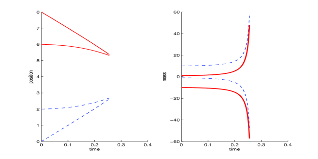
Figure 1: Two symmetric peakon-antipeakon pairs with masses $m_{1}(0)=10=-m_{4}(0)$, $m_{2}(0)=-1=-m_{3}(0)$ undergo a simultaneous collision.

5 Collisions and shocks

In this section we investigate the behaviour of $m$ and $u$ at the time of collision(s). We start with $m$ and observe that since the collision of peakons occurs in pairs it is sufficient to study a fixed colliding pair $m_{j},m_{j+1}$.

Theorem 5.1.

If $m_{j}$ collides with $m_{j+1}$ at time $t_{c}>0$ and the position $x_{c}$, then

$$\lim_{t\to t_{c}^{-}}(m_{j}(t)\delta(x-x_{j}(t))+m_{j+1}(t)\delta(x-x_{j+1}(t)))$$

$$= \left(\lim_{t\to t_{c}^{-}}(m_{j}+m_{j+1})\right)\delta(x-x_{c})+\frac{1}{2}\left(\dot{x}_{j}(t_{c})-\dot{x}_{j+1}(t_{c})\right)\delta^{\prime}(x-x_{c})$$

$$= \left(\lim_{t\to t_{c}^{-}}(m_{j}+m_{j+1})\right)\delta(x-x_{c})+\frac{1}{2}\left(\lim_{t\to t_{c}^{-}}(u(x_{j}(t),t)-u(x_{j+1}(t),t)\right)\delta^{\prime}(x-x_{c})$$

in $\mathscr{D}^{\prime}(\mathbb{R})$.

Proof.

For an arbitrary $\varphi(x)\in\mathscr{D}(\mathbb{R})$,

$$\langle m_{j}(t)\delta(x-x_{j}(t))+m_{j+1}(t)\delta(x-x_{j+1}(t)),\varphi(x)\rangle=m_{j}(t)\varphi(x_{j}(t))+m_{j+1}(t)\varphi(x_{j+1}(t)).$$

Using Corollary 4.9 we can write

$$m_{j}=-\frac{1}{2(t-t_{c})}+C_{0}+O(t-t_{c}),\quad m_{j+1}=\frac{1}{2(t-t_{c})}+\tilde{C}_{0}+O(t-t_{c})$$

around $t_{c}$. Hence

$$\lim_{t\to t_{c}^{-}}\langle m_{j}(t)\delta(x-x_{j}(t))+m_{j+i}(t)\delta(x-x_{j+1}(t)),\varphi(x)\rangle$$

$$= (C_{0}+\tilde{C}_{0})\varphi(x_{c})-\lim_{t\to t_{c}}\frac{\varphi(x_{j}(t))-\varphi(x_{j+1}(t))}{2(t-t_{c})}$$

$$= \left(\lim_{t\to t_{c}^{-}}(m_{j}+m_{j+1})\right)\varphi(x_{c})-\frac{1}{2}\left(\lim_{t\to t_{c}^{-}}(\dot{x}_{j}-\dot{x}_{j+1})\right)\varphi^{\prime}(x_{c})$$

$$= \left(\lim_{t\to t_{c}^{-}}(m_{j}+m_{j+1})\right)\varphi(x_{c})-\frac{1}{2}\left(\lim_{t\to t_{c}^{-}}(u(x_{j}(t),t)-u(x_{j+1}(t),t))\right)\varphi^{\prime}(x_{c}),$$

where in the last step we used equation (2.6a). The conclusion now follows from the definition of $\delta$ and $\delta^{\prime}$. ∎

Since $m=u-u_{xx}$ we have the immediate corollary.

Corollary 5.2.

Suppose $m(0)=2\sum_{k=1}^{n}m_{k}(0)\delta(x-x_{k}(0))$ is a multipeakon at $t=0$ for which $M_{n}\neq 0$ and such that at $t_{c}$ one, or several of its peakon-antipeakon pairs collide. For any colliding pair $k,k+1$ let us denote $\lim_{t\to t_{c}^{-}}u(x_{k}(t))=u_{l}(x_{k}(t_{c})),\;\lim_{t\to t_{c}^{-}}u(x_{k+1}(t)=u_{r}(x_{k}(t_{c}))$ respectively. Then

$$\lim_{t\to t_{c}^{-}}m(t)=2\sum_{k=1}^{n}\tilde{m}_{k}(t_{c})\delta(x-x_{k}(t_{c}))+2\sum_{\begin{subarray}{c}k:\text{pairs}\\ x_{k},x_{k+1}\text{collide}\end{subarray}}s_{k}(t_{c})\delta^{\prime}(x-x_{k}(t_{c}))\;\text{ in }\cal{D}^{\prime}(\mathbf{R}).$$

The shock strengths are given by

$$s_{k}(t_{c})=\frac{u_{l}(x_{k}(t_{c}))-u_{r}(x_{k}(t_{c}))}{2},$$

and they satisfy the (strict) entropy condition $s_{k}(t_{c})>0$.

Proof.

It suffices to prove the claim if there is only one colliding pair; the general case follows easily since masses collide pairwise. For $t<t_{c}$ the measure evolves as $m(t)=2\sum_{k=1}^{n}m_{k}(t)\delta(x-x_{k}(t))$ where $x_{k}(t),m_{k}(t)$ satisfy equations (2.6a), (2.6b) respectively. Suppose now that the pair $j,j+1$ collides at the point $x_{c}$. Then by Theorem 5.1 $\lim_{t\to t_{c}}m(t)=2\sum_{k\neq j,j+1}m_{k}(t_{c})\delta(x-x_{k}(t_{c}))+2\lim_{t\to t_{c}^{-}}(m_{j}+m_{j+1}(t)\delta(x-x_{c})+2\frac{1}{2}(\dot{x}_{j}(t_{c})-\dot{x}_{j+1}(t_{c}))\delta^{\prime}(x-x_{c}).$ To prove that $s_{j}(t_{c})\geq 0$ we write $s_{j}(t_{c})=\frac{1}{2}\lim_{t\to t_{c}^{-}}(\dot{x}_{j}(t)-\dot{x}_{j+1}(t))=\frac{1}{2}\lim_{t\to t_{c}^{-}}(u(x_{j}(t),t)-u(x_{j+1}(t),t))$ and observe

$$\dot{x}_{j}(t_{c})-\dot{x}_{j+1}(t_{c})=\lim_{t\to t_{c}}\frac{x_{j+1}(t)-x_{j}(t)}{t_{c}-t}$$

which implies the entropy condition $s_{j}(t_{c})\geq 0$ in view of the ordering assumption $x_{j}(t)<x_{j+1}(t)$. The strict inequality follows from item (4) in Theorem 4.7. ∎

The following amplification of the previous theorem brings the issues of the wave breakdown and a shock creation sharply into focus. To put our result into the proper perspective we first review the well-posedness result for $L^{1}(\mathbb{R})\cap BV(\mathbb{R})$ proven by Coclite and Karlsen ([4], Section 3). We present only the core result pertinent to our paper.

Theorem 5.3 (Coclite-Karlsen).

Let $u_{0}\in L^{1}(\mathbb{R})\cap BV(\mathbb{R})$. Then there exists a unique entropy weak solution to the Cauchy problem $u|_{t=0}=u_{0}$ for the DP equation (2.1).

It is then proven in [17] that the shockpeakon ansatz

$$u(x,t)=\sum_{j=1}^{n}\{m_{j}(t)-s_{j}(t)\operatorname{sgn}(x-x_{j}(t))\}e^{-|x-x_{j}(t)|},$$

is an entropy weak solution provided the shock strengths $s_{j}\geq 0$. This sets the stage for the next theorem.

Theorem 5.4.

Assume that a multipeakon solution $u(x,t)$ exists on $\mathbb{R}^{n}\times[0,t_{c})$, then $u(\cdot,t)\in L^{1}(\mathbb{R})\cap BV(\mathbb{R})$ for all $0\leq t<t_{c}$ and $u(\cdot,t)$ converges in $L^{1}$ to the shockpeakon

$$u(x,t_{c})=\sum_{i=1}^{n}\tilde{m}_{i}(t_{c})e^{-|x-x_{i}(t_{c})|}+\sum_{i=1}^{n}C_{i}\dot{x}_{i}(t_{c})\mathrm{sgn}(x-x_{i}(t_{c}))e^{-|x-x_{i}(t_{c})|},\quad$$

$u(\cdot,t_{c})\in L^{1}(\mathbb{R})\cap BV(\mathbb{R})$, where $m_{i}(t)$’s Laurent expansion around $t_{c}$ is written as

$$m_{i}(t)=\frac{C_{i}}{t-t_{c}}+\sum_{l=0}^{\infty}a_{l}(t-t_{c})^{l}\stackrel{{\scriptstyle\mathrm{def}}}{{=}}\frac{C_{i}}{t-t_{c}}+\tilde{m}_{i}(t),$$

with the proviso that $C_{i}=0$ if the $i$th mass is not involved in a collision and $C_{i}=-\frac{1}{2}$ for a colliding peakon, $C_{i}=\frac{1}{2}$ for a colliding antipeakon, respectively.

Proof.

We start with the case $n=2$. Then $u(x,t)=m_{1}(t)e^{-|x-x_{1}(t)|}+m_{2}(t)e^{-|x-x_{2}(t)|}$ and $x_{1}(t_{c})=x_{2}(t_{c})=x_{c}$. According to Theorem 4.5, we have

$$m_{1}(t)=-\frac{1}{2(t-t_{c})}+\tilde{m}_{1}(t),\quad m_{2}(t)=\frac{1}{2(t-t_{c})}+\tilde{m}_{2}(t),$$

where $\tilde{m}_{1}(t),\tilde{m}_{2}(t)$ are analytic around $t_{c}$. It is clear that

$$\tilde{m}_{1}(t)e^{-|x-x_{1}(t)|}+\tilde{m}_{2}(t)e^{-|x-x_{2}(t)|}\in L^{1}(\mathbb{R})\cap BV(\mathbb{R})\quad\text{for all $0\leq t\leq t_{c}$}.$$

By the mean value theorem we find that

$$v(x,t)\stackrel{{\scriptstyle\mathrm{def}}}{{=}}\frac{1}{2(t-t_{c})}(e^{-|x-x_{2}(t)|}-e^{-|x-x_{1}(t)|})$$

$$= \left\{\begin{aligned} &\frac{1}{2}\left.\left[\dot{x}_{1}(s)e^{x-x_{1}(s)}-\dot{x}_{2}(s)e^{x-x_{2}(s)}\right]\right|_{s=t+\theta_{1}(t_{c}-t)},&&x<x_{1}(t)<x_{2}(t),\\ &\frac{1}{2}\left.\left[\dot{x}_{2}(s)e^{x_{2}(s)-x}-\dot{x}_{1}(s)e^{x_{1}(s)-x}\right]\right|_{s=t+\theta_{2}(t_{c}-t)},&&x_{1}(t)<x_{2}(t)<x,\\ &\frac{e^{x-x_{c}}-e^{x_{c}-x}}{2(t-t_{c})}-\left.\frac{1}{2}(\dot{x}_{1}(s)e^{x_{1}(s)-x}+\dot{x}_{2}(s)e^{x-x_{2}(s)})\right|_{s=t+\theta_{3}(t_{c}-t)},&&x_{1}(t)<x<x_{2}(t),\end{aligned}\right.$$

where $0<\theta_{j}<1,\;j=1,2,3$. Hence we have the pointwise limit

$$\lim_{t\to t_{c}^{-}}v(x,t)=\begin{cases}\mathrm{sgn}(x-x_{c})(-\frac{1}{2}\dot{x}_{1}(t_{c})+\frac{1}{2}\dot{x}_{2}(t_{c}))e^{-|x-x_{c}|},\;\text{ for }x\neq x_{c},\\ -\frac{\dot{x}_{1}(t_{c})+\dot{x}_{2}(t_{c})}{2},\;\text{ for }x=x_{c}.\end{cases}$$

Let us define

$$v(x,t_{c})=\begin{cases}\mathrm{sgn}(x-x_{c})(-\frac{1}{2}\dot{x}_{1}(t_{c})+\frac{1}{2}\dot{x}_{2}(t_{c}))e^{-|x-x_{c}|},\;\text{ for }x\neq x_{c},\\ 0,\;\text{ for }x=x_{c}.\end{cases}$$

and consider the integral

$$\int\limits_{-\infty}^{+\infty}|v(x,t)-v(x,t_{c})|\mathrm{d}x=\left(\int\limits_{-\infty}^{x_{1}(t)}+\int\limits_{x_{1}(t)}^{x_{2}(t)}+\int\limits_{x_{2}(t)}^{+\infty}\right)|v(x,t)-v(x,t_{c})|\mathrm{d}x.$$

Then the first and the last term of the right hand side converge to zero as $t\to t_{c}^{-}$ due to Lebesgue’s dominated convergence theorem.

Observe that the second term satisfies

$$\int\limits_{x_{1}(t)}^{x_{2}(t)}|v(x,t)-v(x,t_{c})|\mathrm{d}x\leq\int\limits_{x_{1}(t)}^{x_{2}(t)}|v(x,t)|\mathrm{d}x+\int\limits_{x_{1}(t)}^{x_{2}(t)}|v(x,t_{c})|\mathrm{d}x$$

$$\leq \int\limits_{x_{1}(t)}^{x_{2}(t)}|v(x,t)|\mathrm{d}x+\int\limits_{x_{1}(t)}^{x_{2}(t)}\frac{|e^{x-x_{2}(t)}-e^{x_{c}-x}|}{2(t_{c}-t)}\mathrm{d}x+\frac{1}{2}\int\limits_{x_{1}(t)}^{x_{2}(t)}|\dot{x}_{1}(s)|e^{x_{1}(s)-x}\mathrm{d}x+\frac{1}{2}\int\limits_{x_{1}(t)}^{x_{2}(t)}|\dot{x}_{2}(s)|e^{x-x_{2}(s)}\mathrm{d}x$$

$$= \int\limits_{x_{1}(t)}^{x_{2}(t)}|v(x,t)|\mathrm{d}x+\frac{x_{2}(t)-x_{1}(t)}{2(t_{c}-t)}|e^{y-x_{c}}-e^{x_{c}-y}|+\frac{1}{2}\int\limits_{x_{1}(t)}^{x_{2}(t)}|\dot{x}_{1}(s)|e^{x_{1}(s)-x}\mathrm{d}x+\frac{1}{2}\int\limits_{x_{1}(t)}^{x_{2}(t)}|\dot{x}_{2}(s)|e^{x-x_{2}(s)}\mathrm{d}x$$

where $s\in(t,t_{c})$ and $y\in(x_{1}(t),x_{2}(t))$. Since $|\dot{x}_{1}(s)|e^{x_{1}(s)-x}$ and $|\dot{x}_{2}(s)|e^{x-x_{2}(s)}$ are bounded, and

$$x_{2}(t)-x_{1}(t)\to 0,\quad\frac{x_{2}(t)-x_{1}(t)}{2(t_{c}-t)}\to\dot{x}_{1}(t_{c})-\dot{x}_{2}(t_{c}),\quad|e^{y-x_{c}}-e^{x_{c}-y}|\to 0$$

as $t\to t_{c}^{-}$, we have that $v(x,t)$ converges to $v(x,t_{c})$ in the sense of $L^{1}$, which shows that the conclusion holds for $n=2$.

In general, since collisions can only occur in pairs, we can assume that $m_{j_{1}}(t),m_{j_{1}+1}(t),m_{j_{2}}(t),m_{j_{2}+1}(t),\ldots,m_{j_{k}}(t),m_{j_{k}+1}(t)$ blow up at $t_{c}$ and all the other $m_{i}$’s remain bounded. It is clear that $m_{i}(t)e^{-|x-x_{i}(t)|}$ lies in $L^{1}(\mathbb{R})\cap BV(\mathbb{R})$ and converges to $m_{i}(t_{c})e^{-|x-x_{i}(t_{c})|}$ in $L^{1}$ if $m_{i}(t)$ remains bounded at $t_{c}$. Meanwhile, according the proof above, we can easily see that

$$m_{j_{s}}(t)e^{-|x-x_{j_{s}}(t)|}+m_{j_{s}+1}(t)e^{-|x-x_{j_{s}+1}(t)|}\in L^{1}(\mathbb{R})\cap BV(\mathbb{R})\quad\text{for all $1\leq s\leq k$},$$

whose limit is

$$\tilde{m}_{j_{s}}(t_{c})e^{-|x-x_{j_{s}}(t_{c})|}+\tilde{m}_{j_{s}+1}(t_{c})e^{-|x-x_{j_{s}+1}(t_{c})|}$$

$$-\frac{1}{2}\operatorname{sgn}(x-x_{j_{s}}(t_{c}))(\dot{x}_{j_{s}}(t_{c})-\dot{x}_{j_{s}+1}(t_{c}))e^{-|x-x_{j}(t_{c})|}$$

as $t\to t_{c}^{-}$, which leads to the conclusion. ∎

Corollary 5.5.

The limit of a multipeakon $u(\cdot,t)$ for $t\rightarrow t_{c}^{-}$ has a unique entropy weak extension which is a shockpeakon in the sense of H. Lundmark.

6 Acknowledgments

We thank Hans Lundmark for numerous perceptive comments. J. S. would like to thank the Centro Internacional de Ciencias (CIC) in Cuernavaca (Mexico) for hospitality and F. Calogero for making the stay so enjoyable and productive. This work was supported by National Natural Science Funds of China
[NSFC10971155 to L.Z.]; and Natural Sciences and Engineering Research Council of Canada [NSERC163953 to J.S.]. Both authors would like to thank the Department of Mathematics and Statistics of the University of Saskatchewan for making the collaboration possible.

References

- [1] R. Beals, D. Sattinger, and J. Szmigielski. Multipeakons and the classical moment problem. Advances in Mathematics, 154:229–257, 2000.
- [2] R. Beals, D. H. Sattinger, and J. Szmigielski. Multi-peakons and a theorem of Stieltjes. Inverse Problems, 15(1):L1–L4, 1999.
- [3] R. Camassa and D. D. Holm. An integrable shallow water equation with peaked solitons. Phys. Rev. Lett., 71(11):1661–1664, 1993.
- [4] G. M. Coclite and K. H. Karlsen. On the well-posedness of the Degasperis–Procesi equation. J. Funct. Anal., 233(1):60–91, 2006.
- [5] G. M. Coclite and K. H. Karlsen. On the uniqueness of discontinuous solutions to the Degasperis–Procesi equation. J. Differential Equations, 234(1):142–160, 2007.
- [6] G. M. Coclite, K. H. Karlsen, and N. H. Risebro. Numerical schemes for computing discontinuous solutions of the Degasperis-Procesi equation. IMA J. Numer. Anal., 28(1):80–105, 2008.
- [7] A. Constantin and D. Lannes. The hydrodynamical relevance of the Camassa-Holm and Degasperis-Procesi equations. Arch. Ration. Mech. Anal., 192(1):165–186, 2009.
- [8] A. Degasperis, D. D. Holm, and A. N. W. Hone. A new integrable equation with peakon solutions. Theoretical and Mathematical Physics, 133:1463–1474, 2002.
- [9] A. Degasperis and M. Procesi. Asymptotic integrability. In A. Degasperis and G. Gaeta, editors, Symmetry and perturbation theory (Rome, 1998), pages 23–37. World Scientific Publishing, River Edge, NJ, 1999.
- [10] J. Escher, Y. Liu, and Z. Yin. Global weak solutions and blow-up structure for the Degasperis-Procesi equation. J. Funct. Anal., 241(2):457–485, 2006.
- [11] B.-F. Feng and Y. Liu. An operator splitting method for the Degasperis-Procesi equation. J. Comput. Phys., 228(20):7805–7820, 2009.
- [12] E. L. Ince. Ordinary Differential Equations. Dover Publications, New York, 1944.
- [13] R. S. Johnson. Camassa-Holm, Korteweg-de Vries and related models for water waves. J. Fluid Mech., 455:63–82, 2002.
- [14] Z. Lin and Y. Liu. Stability of peakons for the Degasperis-Procesi equation. Comm. Pure Appl. Math., 62(1):125–146, 2009.
- [15] Y. Liu. Wave breaking phenomena and stability of peakons for the Degasperis-Procesi equation. In Trends in partial differential equations, volume 10 of Adv. Lect. Math. (ALM), pages 265–293. Int. Press, Somerville, MA, 2010.
- [16] Y. Liu and Z. Yin. Global existence and blow-up phenomena for the Degasperis-Procesi equation. Comm. Math. Phys., 267(3):801–820, 2006.
- [17] H. Lundmark. Formation and dynamics of shock waves in the Degasperis–Procesi equation. J. Nonlinear Sci., 17(3):169–198, 2007.
- [18] H. Lundmark and J. Szmigielski. Multi-peakon solutions of the Degasperis–Procesi equation. Inverse Problems, 19:1241–1245, December 2003.
- [19] H. Lundmark and J. Szmigielski. Degasperis-Procesi peakons and the discrete cubic string. IMRP Int. Math. Res. Pap., (2):53–116, 2005.
- [20] A. J. Majda and A. L. Bertozzi. Vorticity and incompressible flow, volume 27 of Cambridge Texts in Applied Mathematics. Cambridge University Press, Cambridge, 2002.
- [21] H. P. McKean. Breakdown of a shallow water equation. Asian J. Math., 2(4):867–874, 1998. Mikio Sato: a great Japanese mathematician of the twentieth century.
- [22] H. P. McKean. Breakdown of the Camassa-Holm equation. Comm. Pure Appl. Math., 57(3):416–418, 2004.
- [23] J. Szmigielski and L. Zhou. Peakon-antipeakon interaction in the Degasperis-Procesi equation. http://arxiv.org/abs/1301.0171 [math-ph], 29 pp., 2013.