p-Wave Superconductivity near a transverse saturation field

Abstract

We investigate reentrant superconductivity in an Ising ferromagnetic superconductor URhGe under a transverse magnetic field $h_{x}$. The superconducting transition temperature for $p$-wave order parameters $T_{sc}$ is calculated and shows two domes as a function of $h_{x}$. We find strong enhancement of $T_{sc}$ in the high-field dome near a saturation field $h_{s}$ where the spins align in the transverse direction. Soft magnons generate strong attractive interactions there. Spin components of the pairing show a significant change between $h_{x}$$<$$h_{s}$ and $h_{x}$$>$$h_{s}$. We also discuss the appearance of superconductivity with zero-spin pair due to cancellation between external and exchange fields.

Ferromagnetic superconductivity (SC) has attracted much attention in condensed matter physics in the last decade.AokiFlouquet U-based heavy-fermion compounds such as UGe₂, URhGe, UIr, and UCoGe show unconventional SC within their ferromagnetic phases.UGe2 ; Aoki ; UIr ; UCoGe Non-unitary SC’sMachida are believed to appear in these compounds and both the SC and ferromagnetism are caused in the $f$ electrons at U sites. Their pairing mechanism and symmetry as well as novel self-induced vortex states are central issues to be clarified in the modern theory of unconventional superconductors.

Two isomorphic compounds, UTGe(T=Rh, Co), exhibit SC at ambient pressure within their ferromagnetic state and have a similar Ising type anisotropy of magnetization.AokiFlouquet ; Knafo Spontaneous moment appears parallel to the $c$-axis and its magnetization curve exhibits meta-magnetism when magnetic field ${\bf H}$ is applied to one of the hard axes ($b$ axis) with a notable mass enhancement.Miyake This meta-magnetism is particularly prominent in URhGe and the moment gradually tilts with field and finally aligns parallel to ${\bf H}$ at $12$ T.LevyHuxley Superconductivity appears below the transition temperature $T_{sc}$$=$$0.24$ K for ${\bf H}$$=$${\bf 0}$, and $T_{sc}$ decreases with ${\bf H}$ and disappears at $2$ T for $\bf H$ $\parallel b$.LevyHuxley Interestingly, SC reappears above $8$ T and shows the highest $T_{sc}$$=$$0.42$ K at $12$ T.LevyHuxley

Theories of ferromagnetic SC have been developed by various groups,Fay ; Kirk ; Mineev1 ; Mineev2 ; Tada ; KlemmArXiv especially for UGe₂.Sandman ; Nev ; Linder ; Uz In this paper, we focus on the reentrant SC in URhGe, which has not been investigated theoretically. The physics of the reentrant SC is quite different from that in UGe₂.Sandman ; Nev ; Linder The point is the presence of soft magnons in the Ising systems with transverse fields. We clarify it by extending the Scharnberg-Klemm (SK) theorySK in the presence of ferromagnetism and transverse magnetic fields. In particular, we demonstrate (i) strong enhancement of $T_{sc}$ near the saturation field, and (ii) strong field dependence in spin components ($d$-vector) of $p$-wave pairing.

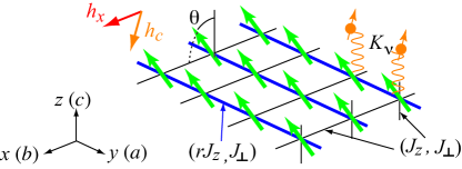
Figure 1: (Color online) Schematic picture of the model.

We consider a system of conduction electrons as shown in Fig. 1, coupled to ferromagnetic localized spins, which have a magnetization ${\bf M}$ in the $z$-direction (corresponding to the $c$ axis in URhGe at ${\bf H}$$=$${\bf 0}$). We apply a transverse magnetic field $H_{x}$ along the $b$ axis and study its effects on ferromagnetic SC. For conduction electrons, we use isotropic dispersion $\varepsilon_{\bf p}$$=$${\bf p}^{2}/2m^{*}$, ignoring complex band structures.bandcalc Here, ${\bf p}$ and $m^{*}$ are the momentum and the effective mass, respectively.

To model spin fluctuations in URhGe, we employ a simple model that can describe their essential behavior, and that is the ferromagnetic XXZ model.single To discuss SC, we will later introduce couplings between localized spins and conduction electrons. We treat local and itinerant degrees of freedom separately and this is qualitatively justified in the “duality” picture.Kuramoto There, ordered moments are due to the incoherent part of $f$ electrons, while itinerant physics such as SC is described by quasiparticles with heavy effective mass $m^{*}$. In this paper, we denote magnetic moments and indices of the Kramers pairs simply as “spin,” but remember that these are complex combinations of orbital and spin moments in heavy-fermion systems.

The ferromagnetic XXZ model for localized moments is given as

$$H_{S}\!\!\! = \!\!\!-\sum_{\langle i,j\rangle}\Big{[}J^{z}_{ij}S_{i}^{z}S_{j}^{z}+J_{\perp}\sum_{\nu=x,y}S_{i}^{\nu}S_{j}^{\nu}\Big{]}-Sh_{x}\sum_{i}S_{i}^{x},\ \ \ \$$ (1)

where the spins ${\bf S}_{i}$ with ${\bf S}_{i}^{2}$$=$$S(S+1)$ are defined on a three-dimensional cubic lattice and $h_{x}$$\equiv$$\mu H_{x}/S$. $\mu$$=$$0.4\mu_{B}$ is the value of magnetic moment measured in experiment,Aoki where $\mu_{B}$ is the Bohr magneton. We have introduced spatial anisotropy $J_{ij}^{z}$ as well as Ising spin anisotropy $J_{ij}^{z}$$>$$J_{\perp}$$>$$0$ as shown in Fig. 1, since the crystal structure can be regarded as coupled-chains running in the $y(a)$ direction: $J_{ij}^{z}$$=$$J_{z}$ for bonds along $\hat{x}$ or $\hat{z}$, while $rJ_{z}$ along $\hat{y}$ with $r>0$. This spatial anisotropy lifts degeneracy in $p$-wave superconducting order parameters as will be discussed later. Although the tetragonal symmetry of the exchange couplings is higher than the orthorhombic one in URhGe, this is not essential for our discussions.

We analyze the model (1) for zero temperature $T$$=$$0$ by the linearized spin-wave approximation.SWA Due to the Ising anisotropy, the spontaneous moment points along $\hat{z}$ at $h_{x}$$=$$0$. As $h_{x}$ increases, the magnetization tilts toward $\hat{x}$ with polar angle $\theta$$=$$\sin^{-1}(h_{x}/h_{s})$ up to the saturation field $h_{s}$$=$$(4+2r)J_{z}-6J_{\perp}$. Magnons defined below describe transverse fluctuations around this tilted direction.

The magnon energy dispersion is expressed as $E_{\bf q}$$=$$S\sqrt{{\epsilon_{\bf q}^{2}-4v_{\bf q}^{2}}},$ where $\epsilon_{\bf q}$$=$$(c_{\theta}^{2}$$-$$s_{\theta}^{2}/2)h_{s}$$+$$h_{x}s_{\theta}$$-$$J_{\perp}(c_{\theta}^{2}$ $+$$1)\gamma_{\bf q}$$-$$J_{z}s_{\theta}^{2}\gamma_{\bf q}^{y}$, $2v_{\bf q}$$=$$s_{\theta}^{2}(h_{s}/2$$+$$J_{z}\gamma_{\bf q}^{y}$$-$$J_{\perp}\gamma_{\bf q})$ with $\gamma_{\bf q}$$=$$\sum_{l=x,y,z}$$(\cos q_{l}$$-$$1)$, $\gamma_{\bf q}^{y}$$=$$\gamma_{\bf q}$$+$$(r$$-$$1)$$(\cos q_{y}$$-$$1)$, and $c_{\theta}(s_{\theta})$$=$$\cos\theta(\sin\theta)$. The dispersion has an energy gap $S\sqrt{h_{s}^{2}-h^{2}_{x}}$ for $h_{x}$$<$$h_{s}$ and $S\sqrt{h_{x}(h_{x}-h_{s})}$ for $h_{x}$$>$$h_{s}$. At $h_{x}$$=$$h_{s}$, the excitations are gapless $E_{\bf q\sim 0}$$\sim$$S\sqrt{h_{s}J_{z}(q_{x}^{2}+rq_{y}^{2}+q_{z}^{2})}$. Note that the model (1) is ferromagnetic, and thus the linearized spin-wave approximation is fairly good even near $h_{s}$. Since the magnitude of $S$ does not play an important role in our approximation, we set $S$$=$$1$. The renormalization of moment due to the quantum fluctuation is small and we neglect it hereafter.

Let us investigate the interactions of magnons and conduction electrons (quasiparticles). The quasiparticles feel the external field and exchange field via anisotropic antiferromagnetic Kondo coupling $K_{x,y,z}$: $\sum_{i\nu}K_{\nu}s_{i}^{\nu}S_{i}^{\nu}$ with $s_{i}^{\nu}$ being the spin of the quasiparticle at the site $i$. Again, note that this “spin” is, indeed, “pseudospin”. Thus, in the mean field level, their energy dispersion is $\varepsilon_{\bf p\pm}$$=$$\varepsilon_{\bf p}\pm|{\bf h}_{c}|/2$ with ${\bf h}_{c}$$=$$(h_{c}^{x},0,h_{c}^{z})$$\equiv$$(\mu_{c}H_{x}$$-$$K_{x}s_{\theta},$$0,-K_{z}c_{\theta})$. Here, $\mu_{c}$$\equiv$$g^{*}\mu_{B}$ with the effective $g$-factor of quasiparticles $g^{*}$.

The lowest-order fluctuations beyond the mean-field approximation yield a magnon-quasiparticle interaction: $\sum_{i\nu}$$v_{\nu}a_{i}^{\dagger}{\tilde{s}}_{i}^{\nu}$+H.c., where $a^{\dagger}_{i}$ is a magnon creation operator at the site $i$ and $\tilde{s}_{i}^{\nu}$ is the quasiparticle spin rotated such that the new $z$-axis is parallel to $-{\bf h}_{c}$. The coupling constant $v_{\nu}$ is given as $(v_{x},v_{y},v_{z})$$=$$(K_{z}s_{\theta}\hat{h}_{c}^{x}$$+$$K_{x}c_{\theta}\hat{h}_{c}^{z}$,$-iK_{y},$$K_{z}s_{\theta}\hat{h}_{c}^{z}$$-$$K_{x}c_{\theta}\hat{h}_{c}^{x})/\sqrt{2}$ with $\hat{h}_{c}^{x,z}$$\equiv$$h^{x,z}_{c}/|{\bf h}_{c}|$.

Next, we derive linearized gap equations for $p$-wave SCSK and determine the transition temperature $T_{sc}$ and upper critical field $H_{c2}$. Since we are mainly interested in high-field states, we neglect small $4\pi{\bf M}$ less than $\sim$ 1 kG in the magnetic induction.Mineev1 This must be taken into account near $h_{x}$$=$$0$ and is important for discussions about self-induced vortex states, which is one of our future problems. Since ${\bf H}\parallel\hat{x}$, the gap equation for the $p_{x}$ state $\vec{\Delta}_{xN}$$=$$[\Delta_{xN}^{++},\Delta_{xN}^{--},\Delta_{xN}^{0}]^{T}$ and the other orbitals $\{\vec{\Delta}_{yN},\vec{\Delta}_{zN}\}$ are decoupled, where $N$ represents the Landau level (LL), and “$++$”, “$--$”, and “$0$” denote the spin projection of Cooper pairs along $-{\bf h}_{c}$. Different LL’s for the $p_{x}$ state are decoupled to each other, while they are coupled for the $(p_{y},p_{z})$ components. In the SK theory, the linearized gap equations are given asSK

$$\vec{\Delta}_{\alpha N}=\frac{3T{m^{*}}^{2}}{2\pi}\hat{V}_{\alpha}\sum_{N^{\prime},\beta}\hat{S}_{NN^{\prime}}^{\alpha\beta}\vec{\Delta}_{\beta N^{\prime}},\quad(\alpha,\beta\in\{x,y,z\}).$$ (2)

Here, $\hat{V}_{\alpha}$ is an interaction matrix of the spin part [see Eq.(3)] for the $p_{\alpha}$ state. $\hat{S}$ includes both the Zeeman and orbital pair breaking effects and is diagonal in spin space.

$\hat{V}_{\alpha}$ is determined from the one-magnon exchange processes and we calculate this with the static approximation for the magnon Green’s function $D_{\bf q}(i\omega_{m})$$=$$1/(i\omega_{m}-E_{\bf q})$$\sim$$-1/E_{\bf q}$. Averaging all the momentum dependence assuming $p$-wave gap functions $\eta_{\bf p}^{\alpha}$, $\hat{V}_{\alpha}$ is given as

$$\hat{V}_{\alpha}\!\!\! = \!\!\!A_{\alpha}^{+}v_{z}^{2}\!\begin{pmatrix}1&w^{2}&\sqrt{2}w\\ w^{2}&1&-\sqrt{2}w\\ \sqrt{2}w&-\sqrt{2}w&w^{2}-1\\ \end{pmatrix}+A_{\alpha}^{-}v_{y}^{2}\begin{pmatrix}0&1&0\\ 1&0&0\\ 0&0&-1\end{pmatrix},$$ (3)

$$\equiv A_{\alpha}^{+}v_{z}^{2}\hat{V}_{+}(w)+A_{\alpha}^{-}v_{y}^{2}\hat{V}_{-},$$

where $w$$=$$v_{x}/v_{z}$ and the first and the second columns of $\hat{V}_{\alpha}$ represent the equal spin pairing (ESP) with the spin function $|$$++\rangle$ and $|$$--\rangle$, respectively, while the third one represents the zero-spin pairing (ZSP) state $(|$$+-\rangle$$+$$|$$-+\rangle)/\sqrt{2}$. Note that “$-$” and “$+$” denote spins parallel and antiparallel to ${\bf h}_{c}$, respectively. Here,

$$A_{\alpha}^{\pm} \equiv \frac{1}{N_{L}^{2}}\sum_{\bf p,k}\eta_{\bf p}^{\alpha}\frac{e^{\pm 2\phi_{\bf p-k}}}{E_{\bf p-k}}\eta_{\bf k}^{\alpha},$$ (4)

where the pairing form factor is chosen as $\eta_{\bf p}^{\alpha}$$=$$\sqrt{2}\sin p_{\alpha}$ and this corresponds to $\sqrt{3}p_{\alpha}$ in continuum systems.SK $\phi_{\bf p-k}$ is related to the Bogoliubov transformation: $\tanh 2\phi_{\bf p-k}$$=$$2v_{\bf p-k}/\epsilon_{\bf p-k}$, and $N_{L}$ is the number of sites.

Before showing numerical results, we analyze $\hat{V}_{\alpha}$ for $h_{x}\sim h_{s}$. Since $E_{\bf q}$ is small around ${\bf q}$$=$${\bf 0}$, $T_{sc}$ is expected to be enhanced. It is important to note that the direction of the local moments continuously changes toward $\pi/2$ for $h_{x}<h_{s}$, while $\theta$$=$$\pi/2$ above $h_{s}$. Expanded up to first order in $\delta\theta$$=$$\pi/2-\theta$, $\hat{V}_{\alpha}$ is given as

$$\frac{1}{2}\begin{pmatrix}0&A_{\alpha}^{+}K_{z}^{2}-A_{\alpha}^{-}K_{y}^{2}&-\Gamma A_{\alpha}^{+}\delta\theta\\ A_{\alpha}^{+}K_{z}^{2}-A_{\alpha}^{-}K^{2}_{y}&0&\Gamma A_{\alpha}^{+}\delta\theta\\ -\Gamma A_{\alpha}^{+}\delta\theta&\Gamma A_{\alpha}^{+}\delta\theta&A_{\alpha}^{+}K_{z}^{2}+{A_{\alpha}^{-}}K_{y}^{2}\end{pmatrix},$$ (5)

where $\Gamma$$=$$\sqrt{2}K_{z}^{2}\{[\mu_{c}h_{s}/(\mu K_{z})-K_{x}/K_{z}]^{-1}-K_{x}/K_{z}\}$. For $h_{x}$$\geq$$h_{s}$, $\delta\theta$$=$$0$, and the gap equations for ESP and ZSP are decoupled. Note that the interaction is strongest for ZSP, since $A_{\alpha}^{\pm}$$>$$0$. This is natural, since the spin fluctuations are transverse, which scatter quasiparticles with $\pm$ spin into $\mp$ spin states.

Low-field longitudinal fluctuationsT-Hattori also mediate interactions and we introduce a phenomenological ferromagnetic Ising interaction between quasiparticles: $-\sum_{\langle i,j\rangle}J_{cc}^{\alpha}s_{i}^{z}s_{j}^{z}$, with $J_{cc}^{\alpha}$$>$$0$ and $\alpha$$\in$$\{x,y,z\}$ is the direction of $ij$ bond. As before, we include spatial anisotropy: $J^{ij}_{cc}$$=$$J_{cc}$ for bond $\parallel{\hat{x}}$ or ${\hat{z}}$, while $r^{\prime}J_{cc}$ for bond $\parallel\hat{y}$. Then, the interaction kernel (3) is replaced as $\hat{V}_{\alpha}$$\to$ $\hat{V}_{\alpha}+({\hat{h}_{z}^{c}})^{2}J_{cc}^{\alpha}\hat{V}_{+}({\hat{h}_{x}^{c}}/{\hat{h}}_{z}^{c})/4$, with keeping the form (5) essentially unchanged.

Let us discuss the phase diagram of SC in the $T$-$h_{x}$ space determined by our calculations. Figures 2 and 3 show the $h_{x}$-dependence of the SC transition temperature of the $p_{x}$- and $p_{y,z}$-states for the isotropic $(r$$=$$r^{\prime}$$=$$1)$ and anisotropic $(r$$=$$1.2,r^{\prime}$$=$$2)$ cases, respectively. Figure 4 shows the spin part of the pairing, and will be discussed later. Our calculations show two domes of $T_{sc}$ in the phase diagram, and this qualitatively reproduces the experimental data.LevyHuxley One important observation is a strong enhancement and the presence of singularity in the high field dome at $h_{x}$$=$$h_{s}$. This manifests the change in the pairing state. The variations in the spin components are due to competition between the interaction strength and the Pauli depairing effects (PDE’s) and we will examine this point in detail in the following.

Let us investigate how the PDE’s influence pairing states. The PDE in the SK theory originates in the matrix $\hat{S}$ in Eq.(2). For $h_{x}$$>$$h_{s}$, the ESP’s and ZSP are decoupled as discussed above, which simplifies analysis. The PDE is weak when the exchange field nearly cancels the external field $h_{c}^{x}\sim 0$. This is realized at high field, and we expect there the ZSP state, since the corresponding interactions are strongest. This is the Jaccarino-Peter effect,JPeffect which was originally proposed for a rare earth ferromagnetic metal. When the cancellation is not sufficient and thus PDE is strong, the ZSP state is suppressed and the ESP state is favored. If the interactions are much stronger than the effective magnetic field, two ESP components $|$$++\rangle$ and $|$$--\rangle$, have nearly equal amplitude. If the interactions are not so strong, the ESP state with larger density of states (DOS) dominates

For $h_{x}\lower 3.01385pt\hbox{$\ \overset{<}{\sim}\ $}h_{s}$, the situation is more complex. When PDE is strong, the ESP with large DOS is realized as expected also for low field, while for weak PDE all the spin components contribute to the superconducting condensation, since the offdiagonal elements in $\hat{V}_{\alpha}$ are finite.

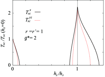
Figure 2: (Color online) Dependence of transition temperature $T_{sc}^{x,yz}$ on transverse field $h_{x}$ for $r$$=$$r^{\prime}$$=$$1$ and $g^{*}$$=$$2$.

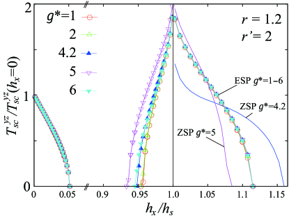
Figure 3: (Color online) $h_{x}$-dependence of $T_{sc}^{yz}$ for the anisotropic case $r$$=$$1.2$, $r^{\prime}$$=$$2$ and five sets of $g^{*}$. The change of low-field dome with $g^{*}$’s is negligible. For $h_{x}$$>$$h_{s}$, the ZSP state is decoupled from the ESP state. Its $T^{yz}_{sc}$ is shown by lines without symbols, except for $g^{*}$$=$$1,2$, and 6, where $T^{yz}_{sc}$ is nearly zero.

Now, we explain the details of Figs. 2–4. Our choice of parameters are: a mean-field ferromagnetic transition temperature $T_{c}^{\rm MF}$$=$$J_{z}(2+r)$$=$$10$ K, $H_{s}$$\equiv$$h_{s}/\mu$$=$$10$ T, $m^{*}/m$$=$$40$, $r^{\prime}J_{cc}$$=$$283$ K, $K_{z}$$=$$109$ K, and $K_{x,y}$$=$$0.3K_{z}$, where $m$ is the bare electron mass. Electron density is set to 1 per unit cell and the lattice constantAoki is set to $3.5$ Å. Using these parameters, $T_{sc}$ at $h_{x}$$=$$0$ is $\simeq$$0.6$ K for both parameter sets in Figs. 2 and 3.logOm $g^{*}$ is the control parameter in our analysis below, which varies the Zeeman energy for quasiparticles.

Let us first examine the orbital part of pairing. The orbital motion couples only to the external field $H_{x}$ as we mentioned above. Therefore, the $p_{x}$-pairing is always decoupled from the other orbitals and different LL’s are decoupled there, while the $p_{y}$ and $p_{z}$ orbitals are mutually coupled with LL’s also coupled. In the isotropic systems, the polar $p_{x}$-state with $N$$=$$0$ has the highest $H_{c2}$ as shown in Fig. 2. We note that the $N$$=$$0$ LL plays a central role in both $p_{x}$ and $p_{y,z}$ states.SK

When the interactions are spatially anisotropic in space with $r,r^{\prime}$$\geq$$1$, the $p_{x}$ state is suppressed and a $p_{y}$-dominant state becomes stable, and vice versa for $r,r^{\prime}$$\leq$$1$. In the following, we analyze the former case, which is relevant for URhGe. Figure 3 shows $T_{sc}^{yz}$ for $r$$=$$1.2$ and $r^{\prime}$$=$$2$, as a typical case of strong anisotropies, for several values of $g^{*}$. Here, $T_{sc}^{x}\ll T_{sc}^{yz}$ for all the parameters and not shown. For the low-field SC, a $p_{y}$ dominant state has a lower energy even for small $r^{\prime}$$\ \overset{>}{\sim}\$$1.05$, while less sensitive to $r$. This is because that the magnon gap is sufficiently large there and thus the transverse fluctuations are negligible. For the high-field SC, both $r$ and $r^{\prime}$ affect its $T_{sc}$. Increasing $r$ enhances $T_{sc}^{yz}$, while it suppresses $T_{sc}^{x}$. For the dependence on $r^{\prime}$, increasing $r^{\prime}$ suppresses both $T_{sc}$’s. The suppression is stronger for $T^{x}_{sc}$ than for $T_{sc}^{yz}$ because the attractive force does not decrease for $p_{y}$ pairs. It is also possible to realize a transition in the SC from $p_{x}$ to $p_{y,z}$ symmetry or vice versa, as $h_{x}$ increases, which is determined by the details of the anisotropies.

Second, we discuss the spin part of pairing, which is related to the $d$-vector of SC, and examine for the data in Fig. 3 the Zeeman effects with controlling $g^{*}$. Figure 4 shows the change in the spin part of pairing with $h_{x}$ for the orbital component $p_{y}$ and $N$$=$$0$ LL. They are calculated just at $T_{sc}^{yz}$ and normalized as $\sum_{N}$$\sum_{\alpha}$$|\vec{\Delta}_{\alpha N}|^{2}$$=$$1$. Figure 4(a) shows the change in the low-field dome. We find that the $g^{*}$-dependence is negligible and the pairing is the ESP state with only one type of spin, which is parallel to the internal field ${\bf h}_{c}$, $|$$--\rangle$. This is consistent with

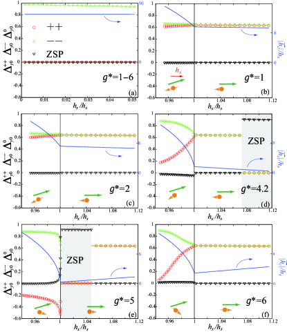
Figure 4: (Color online) Spin part of $p_{y}$ pairing in the $N$$=$$0$ LL for $r$$=$$1.2$ and $r^{\prime}$$=$$2$: $\Delta_{y0}^{++}(\bigcirc)$, $\Delta_{y0}^{--}(\bigtriangleup)$, and $\Delta_{y0}^{0}(\bigtriangledown)$ at $T$$=$$T_{sc}^{yz}$. Lines represent $|{\bf h}_{c}|$. (a) Low-field part, $g^{*}$-dependence is negligible. (b)–(f) High-field part near $h_{s}$ for various $g^{*}$’s. Localized moment (long arrow) and quasiparticle spin (short one with dot) are schematically shown. The magnitude of the quasiparticle spin is small $\leq 0.05$ near $h_{s}$.

the proposed gap symmetry for URhGe.HardyHuxley Figures 4(b)–4(f) show the results in the high-field dome. The region of $h_{x}$$>$$h_{s}$ is, in most of the cases, also the pure ESP state, but now the two spin components have almost the same amplitude. This is because $|$$++\rangle$ pairs are scattered only to $|$$--\rangle$ pairs and vice versa, when $h_{x}$$>$$h_{s}$. However, their amplitude difference may become larger depending on $g^{*}$ and $|{\bf h}_{c}|$. In the region of $h_{x}$$<$$h_{s}$, a small amplitude of the ZSP component hybridizes. The two ESP components are still dominant, but their difference is now larger and the $h_{x}$-dependence is noticeable, particularly for larger $g^{*}$’s. For all $g^{*}$’s, transverse spin fluctuations near $h_{s}$ favor the linear combinations of two ESP states, while ZSP is suppressed by the PDE, except for some regions in Figs. 4(d) and 4(e) as we discuss below.

The quasiparticle spins respond to both the exchange field of the localized moments and the external magnetic field, and $g^{*}$ controls the latter part. Thus, varying $g^{*}$ affects the angle between the quasiparticle and the localized spins as schematically depicted in Figs. 4(b)–4(f). When the external and exchange fields are canceled, ${\bf h}_{c}$$=$${\bf 0}$, the quasiparticle spins feel no field. Indeed, the cancellation can become nearly perfect for $g^{*}$$=$$4.2$ and $5$. This leads to emergence of ZSP states (Jaccarino-Peter effect),JPeffect and occurs in the shaded regions in Figs. 4(d) and 4(e). When $h_{s}$ is close to the point $|{\bf h}_{c}|$$\sim$$0$ as in Fig. 4(e), the expansion in Eq.(5) is not sufficient, and this results in the almost vertical slope of $\vec{\Delta}_{y0}$ for $h_{x}$$\ \overset{<}{\sim}\$$h_{s}$, but this situation is not of main interest in this paper.

Let us finally comment about URhGe. We have succeeded in reproducing the overall phase diagram and two SC domes as shown in Figs. 2 and 3. The transition temperature for the second dome shows strong enhancement near $h_{s}$. The superconducting gap symmetry is basically equal-spin $p_{y(a)}$-pairing for both domes. It is $|$$--\rangle$ for the low-field, and $\sim($$|$$++\rangle$$+$$|$$--\rangle$$)/\sqrt{2}$ for the high-field SC. The gap functions have a point node due to the finite $ip_{z}$ component, but since its amplitude is very small, it might be difficult to experimentally distinguish this from that with a line node. Detecting the change in the spin components of pairing near $h_{s}$ is an experimental test for the present theory. Exploring the sudden change in pairing symmetry due to the Jaccarino-Peter effect is another interesting challenge in this field.

For a more precise theoretical analysis, one should take into account the optimization of form factor $\eta_{\bf k}^{\alpha}$, longitudinal spin fluctuations for $h_{x}\lower 3.01385pt\hbox{$\ \overset{<}{\sim}\ $}h_{s}$,LevyHuxley the weak first-order transition,LevyHuxley the variations of the Fermi surfaces near $h_{s}$,Lif and anisotropy in the effective mass,KlemmArXiv which might improve quantitative agreement between our theory and experiments. Our main conclusion for the superconducting order parameters for $h_{x}$$\sim$$h_{s}$ is that the pairing interaction prefers mixing $|$$++\rangle$ and $|$$--\rangle$ and this is in clear contrast to nearly pure $|$$--\rangle$ state, which is selected by Zeeman energy. Difference in their amplitudes depends on the details, and a more quantitative analysis about this is one of our future plans.

K. H. thanks Dai Aoki for fruitful discussions. He is supported by KAKENHI (No.​ 30456199) and by a Grant-in-Aid for Scientific Research on Innovative Areas “Heavy Electrons” (No.​ 23102707) of MEXT, Japan.

References

- (1) See, recent review: D. Aoki and J. Flouquet: J. Phys. Soc. Jpn. 81, 011003 (2012).
- (2) S. S. Saxena, P. Agarwal, K. Ahilan, F. M. Grosche, R. K. W. Haselwimmer, M. J. Steiner, E. Pugh, I. R. Walker, S. R. Julian, P. Monthoux, G. G. Lonzarich, A. Huxley, I. Sheikin, D. Braithwaite, and J. Flouquet, Nature 406, 587 (2000).
- (3) D. Aoki, A. Huxley, E. Ressouche, D. Braithwaite, J. Flouquet, J.-P. Brison, E. Lhotel, and C. Paulsen, Nature 413, 613 (2001).
- (4) T. Akazawa, H. Hidaka, H. Kotegawa, T. C. Kobayashi, T. Fujiwara, E. Yamamoto, Y. Haga, R. Settai, and Y. Ōnuki J. Phys. Soc. Jpn. 73, 3129 (2004).
- (5) N. T. Huy, A. Gasparini, D. E. de Nijs, Y. Huang, J. C. P. Klaasse, T. Gortenmulder, A. de Visser, A. Hamann, T. Görlach, and H. v. Löhneysen, Phys. Rev. Lett. 99, 067006 (2007).
- (6) T. Ohmi and K. Machida, Phys. Rev. Lett. 71, 625 (1993).
- (7) W. Knafo, T. D. Matsuda, D. Aoki, F. Hardy, G. W. Scheerer, G. Ballon, M. Nardone, A. Zitouni, C. Meingast, and J. Flouquet, Phys. Rev. B 86, 184416 (2012).
- (8) A. Miyake, D. Aoki, and J. Flouquet, J. Phys. Soc. Jpn. 77, 094709 (2008).
- (9) F. Lévy, I. Sheikin, and A. Huxley, Nat. Phys. 3, 460 (2007), F. Lévy, I. Sheikin, B. Grenier, C. Marcenat, and A. Huxley, J. Phys. Condens. Matter 21, 164211 (2009).
- (10) D. Fay and J. Appel, Phys. Rev. B 22, 3173 (1980).
- (11) T. R. Kirkpatrick and D. Belitz, Phys. Rev. B 67, 024515 (2003).
- (12) V. P. Mineev, Phys. Rev. B 66, 134504 (2002), K. V. Samokhin and M. B. Walker, Phys. Rev. B 66, 174501 (2002).
- (13) V. P. Mineev, Phys. Rev. B 81, 180504(R) (2010), ibid., 83, 064515 (2011).
- (14) Y. Tada, N. Kawakami, and S. Fujimoto, J. Phys. Soc. Jpn. 80, SA006 (2011).
- (15) C. Lörscher, R. A. Klemm, J. Zhang, and Q. Gu, arXiv:1110.6667, C. Lörscher, J. Zhang, Q. Gu, and R. A. Klemm, arXiv:1210.7442.
- (16) K. G. Sandeman, G. G. Lonzarich, and A. J. Schofield, Phys. Rev. Lett. 90, 167005 (2003).
- (17) A. H. Nevidomskyy, Phys. Rev. Lett. 94, 097003 (2005).
- (18) J. Linder, I. B. Sperstad, A. H. Nevidomskyy, M. Cuoco, and A. Sudbø, Phys. Rev. B 77, 184511 (2008).
- (19) D. V. Shopova and D. I. Uzunov, Phys. Rev. B 79, 064501 (2009).
- (20) K. Scharnberg and R. A. Klemm, Phys. Rev. B 22, 5233 (1980).
- (21) M. Divis̆, L. M. Sandratskii, M. Richter, P. Mohn, P. Novák, J. Alloys Compd. 337, 48 (2002), A. B. Shick, Phys. Rev. B 65, 180509(R) (2002).
- (22) Essentially the same results are obtained in presence of single-ion anisotropy.
- (23) Y. Kuramoto and K. Miyake, J. Phys. Soc. Jpn, 59, 2831 (1990).
- (24) T. Holstein and H. Primakoff, Phys. Rev. 58, 1098 (1940).
- (25) T. Hattori, Y. Ihara, Y. Nakai, K. Ishida, Y. Tada, S. Fujimoto, N. Kawakami, E. Osaki, K. Deguchi, N. K. Sato, and I. Satoh, Phys. Rev. Lett. 108, 066403 (2012).
- (26) V. Jaccarino and M. Peter, Phys. Rev. Lett. 9, 290 (1962).
- (27) We have introduced a cutoff , where denotes spectral average measured by ; P. B. Allen and R. C. Dynes, Phys. Rev. B 12, 1027 (1975).
- (28) F. Hardy and A. D. Huxley, Phys. Rev. Lett. 94, 247006 (2005).
- (29) E. A. Yelland, J. M. Barraclough, W. Wang, K. V. Kamenev, and A. D. Huxley, Nat. Phys. 7, 890 (2011).