Squeezed primordial bispectrum from general vacuum state

Abstract

We study the general relation between the power spectrum and the squeezed limit of the bispectrum of the comoving curvature perturbation produced during single-field slow-roll inflation when the initial state is a general vacuum. Assuming the scale invariance of the power spectrum, we derive a formula for the squeezed limit of the bispectrum, represented by the parameter ${f_{\rm NL}}$, which is not slow-roll suppressed and is found to contain a single free parameter for a given amplitude of the power spectrum. Then we derive the conditions for achieving a scale-invariant ${f_{\rm NL}}$, and discuss a few examples.

I Introduction

Currently inflation is regarded as the leading candidate to provide the initial conditions for the hot big bang evolution of the universe inflation . During inflation the primordial curvature perturbation is generated, which after inflation becomes seeds for the temperature fluctuations in the cosmic microwave background (CMB) and the large scale structures of the universe. Recent observations Bennett:2012fp are consistent with the predictions of inflation, i.e. the primordial fluctuations are statistically almost perfectly Gaussian with a nearly scale invariant power spectrum. Thus, one of the main tasks of ongoing and future observation programmes such as PLANCK :2006uk is to test if there is any deviation from these predictions. These high precision future observations will able us to rule out and/or further constrain various models of inflation, thus shedding light on the physics of the very early universe.

Among observable signatures, non-Gaussianity has been attracting great interest. In particular a lot of efforts have been made to detect a non-zero three-point correlation function, or its Fourier transform, the bispectrum, of the primordial perturbation nGreviews . The bispectrum is specified by three parameters, and templates for various configurations in the momentum space have been proposed and used in observation. Among them, a particularly useful one is the squeezed configuration, where one of three momenta is much smaller than the others, e.g. $k_{1}\approx k_{2}\gg k_{3}$. A dominant source of non-Gaussianity for this configuration is the so-called local one, where the curvature perturbation is locally expanded as Komatsu:2001rj ; Maldacena:2002vr

$${\cal R}(x)={\cal R}_{g}(x)+\frac{3}{5}{f_{\rm NL}}{\cal R}_{g}^{2}(x)+\cdots\,,$$ (1)

where the subscript $g$ denotes the dominant Gaussian component. The coefficient ${f_{\rm NL}}$ determines the size of non-Gaussianity in the bispectrum.

An important prediction of single-field slow-roll inflation is that, in the squeezed limit, ${f_{\rm NL}}$ is proportional to the spectral index $n_{\cal R}-1$ of the power spectrum Maldacena:2002vr ; Creminelli:2004yq , and is thus too small to be observed. This relation holds irrespective of the detail of models and is usually called the consistency relation. Thus, barring the possibility of features that correlate the power spectrum and ${f_{\rm NL}}$ Achucarro:2012fd , it has been widely claimed that any detection of the local non-Gaussianity would rule out all single field inflation models. However, it is based on two assumptions. First, the curvature perturbation is frozen outside the horizon and does not evolve. That is, only one growing mode is relevant on super-horizon scales. Indeed, it is possible to make use of the constancy of ${\cal R}$ to extract only a few relevant terms in the cubic order Lagrangian to simplify considerably the calculation of the squeezed bispectrum, and to confirm the consistency relation longshortsplit . If we abandon this assumption, the usual consistency relation does not hold any longer noconstancy .

Another assumption is that deep inside the horizon interactions are negligible and the state approaches the standard Fock vacuum in the Minkowski space, so-called the Bunch-Davies (BD) vacuum. If this assumption does not hold, the corresponding bispectrum may be enhanced in the folded limit nBDfolded , in particular in the squeezed limit nBDsqueezed ; nBDmodel . Thus, the usual consistency relation may not hold. See also TanakaUrakawa , where the violation of the tree level consistency relation is discussed together with the infrared divergence in the power spectrum from one-loop contributions for non-BD initial states. However, in the previous studies the relation between the power spectrum and bispectrum was unclear and ${f_{\rm NL}}$ was not easily readable nBDsqueezed , or case studies on specific models were carried out nBDmodel . It is then of interest to make a closer and more explicit study on the general relation between the power spectrum and the squeezed limit of the bispectrum.

In this article, we compute the squeezed limit of the bispectrum when the initial state is not the BD vacuum and study the relation between the squeezed limit of the primordial bispectrum, described by the non-linear parameter ${f_{\rm NL}}$ and the power spectrum. We find indeed ${f_{\rm NL}}$ can be significantly large, but its momentum dependence is in general non-trivial. We then discuss the condition for ${f_{\rm NL}}$ to be momentum-independent, thus exactly mimics the local form (1).

Before proceeding to our analysis, let us make a couple of comments. First, we note that the squeezed limit does not necessarily mean the exact limit of a squeezed triangle in the momentum space. It includes the case when the wavenumber of the squeezed edge of a triangle is smaller than that of the observationally smallest possible wavenumeber, i.e. that corresponds to the current Hubble parameter. In the context of (1), it needs to be valid only over the region covering our current Hubble horizon size. Second, in our analysis we focus only on the squeezed limit of the bispectrum and its relation to the power spectrum. However, if a large ${f_{\rm NL}}$ that mimics the local form of the non-Gaussianity is generated, we may also have the bispectrum with a non-negligible amplitude in some other shapes of the triangle nBDsqueezed ; nBDmodel . This may be an interesting issue to be studied, but it is out of the scope of this work.

II Bispectrum in single-field slow-roll inflation

For general single-field inflation, the equation of motion of the comoving curvature perturabation ${\cal R}$ is given by Garriga:1999vw

$$\left(z^{2}{\cal R}_{k}^{\prime}\right)^{\prime}+c_{s}^{2}k^{2}z^{2}{\cal R}_{k}=0\,,$$ (2)

where a prime denotes a derivative with respect to the conformal time $d\tau=dt/a$, $\epsilon\equiv-\dot{H}/H^{2}$ and $z^{2}\equiv 2m_{\rm Pl}a^{2}\epsilon/c_{s}^{2}$ and $c_{s}$ is the speed of sound. From (2), we can see that irrespective of the detail of the matter sector, a constant solution of ${\cal R}_{k}$ always exists on super-sound-horizon scales, $c_{s}k\ll aH$, and it dominates at late times for slow-roll inflation for which $z^{-1}\sim a^{-1}\sim\tau$.

Here we focus on the case of slow-roll inflation. Keeping the constancy of ${\cal R}_{k}$ on large scales, in the squeezed limit $k_{1}\approx k_{2}$ and $k_{3}\to 0$, the bispectrum at $\tau=\bar{\tau}$ is given by longshortsplit

$$B_{\cal R}(k_{1},k_{2},k_{3};\bar{\tau}) =\left[\frac{\eta(\bar{\tau})}{c_{s}^{2}(\bar{\tau})}+\frac{F(k_{1},\bar{\tau})}{P_{\cal R}(k_{1})}\right]P_{\cal R}(k_{1})P_{\cal R}(k_{3})\,,$$ (3)

$$F(k,\bar{\tau}) =i{\cal R}_{k}^{2}(\bar{\tau})\int_{-\infty}^{\bar{\tau}}d\tau\left[\frac{2\epsilon}{c_{s}^{4}}\left(\epsilon-3+3c_{s}^{2}\right)a^{2}\left({\cal R}_{k}^{\prime*}\right)^{2}+\frac{2\epsilon}{c_{s}^{2}}\left(\epsilon-2s+1-c_{s}^{2}\right)a^{2}k^{2}\left({\cal R}_{k}^{*}\right)^{2}\right.$$

$$\hskip 93.89418pt\left.+\frac{2\epsilon}{c_{s}^{2}}\frac{d}{d\tau}\left(\frac{\eta}{c_{s}^{2}}\right)a^{2}{\cal R}_{k}^{\prime*}{\cal R}_{k}^{*}+\text{c.c.}\right]\,,$$ (4)

where $\eta\equiv\dot{\epsilon}/(H\epsilon)$ and $s\equiv\dot{c}_{s}/(Hc_{s})$.

Being interested in large non-Gaussianity, among the terms inside the square brackets of (II) we may focus on those not suppressed by the slow-roll parameters, that is,

$$F_{0}=\frac{2\left(1-c_{s}^{2}\right)}{c_{s}^{2}}\Re\left\{i{\cal R}_{k}^{2}(\bar{\tau})\int_{-\infty}^{\bar{\tau}}d\tau\left[-3z^{2}\left({\cal R}_{k}^{\prime*}\right)^{2}+c_{s}^{2}k^{2}z^{2}\left({\cal R}_{k}^{*}\right)^{2}\right]\right\}\,,$$ (5)

where for simplicity we have assumed the time variation of $c_{s}^{2}$ is negligible, $s=0$. Now, we find it is more convenient to write the integrand of (5) in terms of ${\cal R}_{k}^{\prime}$. Multiplying (2) by ${\cal R}_{k}$, we have

$$c_{s}^{2}k^{2}z^{2}{\cal R}_{k}^{2}=-\left(z^{2}{\cal R}_{k}^{\prime}{\cal R}_{k}\right)^{\prime}+\left(z{\cal R}_{k}^{\prime}\right)^{2}\,.$$ (6)

Hence (5) becomes

$$F_{0}=\frac{2\left(1-c_{s}^{2}\right)}{c_{s}^{2}}\Re\left\{i{\cal R}_{k}^{2}({\bar{\tau}})\left[-z^{2}{\cal R}_{k}^{*}{\cal R}_{k}^{*\prime}(\bar{\tau})-2\int_{-\infty}^{{\bar{\tau}}}d\tau\,\left(z{\cal R}_{k}^{\prime*}\right)^{2}\right]\right\}\equiv\frac{2\left(1-c_{s}^{2}\right)}{c_{s}^{2}}\left(\Re[I_{1}]+\Re[I_{2}]\right)\,.$$ (7)

As we can write ${\cal R}_{k}$ in terms of ${\cal R}_{k}^{\prime}$ as (2), we do not have to work with ${\cal R}_{k}$ but only need to solve for ${\cal R}_{k}^{\prime}$. Setting

$$f\equiv z{\cal R}_{k}^{\prime}\,,$$ (8)

and taking a derivative of (2), we obtain

$$f^{\prime\prime}+\left[c_{s}^{2}k^{2}-z(z^{-1})^{\prime\prime}\right]f=0\,.$$ (9)

An interesting property of this equation is that in the slow-roll case, $z^{-1}\sim a^{-1}\sim\tau$, so the potential term $z(z^{-1})^{\prime\prime}$ vanishes at leading order Sasaki:1986hm . Specifically we have

$$z(z^{-1})^{\prime\prime}=a^{2}H^{2}\left[\epsilon+\frac{\eta}{2}+{\cal O}(\eta^{2},\epsilon\eta)\right]\,.$$ (10)

This means that the WKB solution $f\propto e^{\pm ic_{s}k\tau}$ remains valid even on super-sound-horizon scales at leading order in the slow-roll expansion. The general leading order solution during slow-roll inflation is thus

$$f=\sqrt{\frac{c_{s}k}{2}}\left(C_{k}e^{-ic_{s}k\tau}+D_{k}e^{ic_{s}k\tau}\right)\,,$$ (11)

where $C_{k}$ and $D_{k}$ are constant and we have extracted the factor $\sqrt{c_{s}k/2}$ for convenience.

Carrying out the standard quantization procedure, we find that for $f$ to be properly normalized, the constants $C_{k}$ and $D_{k}$ satisfy

$$|C_{k}|^{2}-|D_{k}|^{2}=1\,.$$ (12)

Setting $D_{k}=0$ corresponds to the usual choice of the BD vacuum. But here we do not assume so and let $D_{k}$ be generally non-zero. From (6) and (11), the power spectrum can be easily computed to be

$${\cal P}_{\cal R}=\frac{k^{3}}{2\pi^{2}}\left|{\cal R}_{k}\right|_{c_{s}k=aH}^{2}=\frac{k^{3}}{2\pi^{2}}\frac{1}{2(c_{s}k)^{3}}\left(\frac{z^{\prime}}{z^{2}}\right)_{c_{s}k=aH}^{2}\left|C_{k}+D_{k}\right|^{2}\,.$$ (13)

Thus, a scale-invariant spectrum requires $\left|C_{k}+D_{k}\right|^{2}\sim k^{0}$.

Now we return to (7). For slow-roll inflation, ${\cal R}_{k}^{\prime}$ rapidly decays outside the sound horizon. However, since $z$ grows like $a$, neither $I_{1}$ nor $I_{2}$ may not be negligible outside the sound horizon. Rewrite them in terms of $f$, we easily find the expression for $\Re[I_{1}]$ as

$$\Re[I_{1}]=\Re\left[\frac{i}{z^{2}(c_{s}k)^{6}}\left|f^{\prime}+\frac{z^{\prime}}{z}f\right|^{2}f^{\prime}f^{*}\right]=\frac{k^{-3}}{c_{s}^{5}}\left(\frac{z^{\prime}}{z^{2}}\right)^{2}\left|C_{k}+D_{k}\right|^{2}\,,$$ (14)

where we have used (12). The second term is

$$\Re[I_{2}] =\Re\left[-i\frac{2}{z^{2}(c_{s}k)^{4}}\left(f^{\prime}+\frac{z^{\prime}}{z}f\right)^{2}\int_{-\infty}^{{\bar{\tau}}}d\tau\,(f^{*})^{2}\right]$$

$$\approx-\frac{k^{-4}}{z^{2}c_{s}^{5}}\Re\left[\left(f^{\prime}+\frac{z^{\prime}}{z}f\right)^{2}\left({C_{k}^{*}}^{2}e^{2ic_{s}k\bar{\tau}}+{D_{k}^{*}}^{2}e^{-2ic_{s}k\bar{\tau}}-4ic_{s}k{\tau_{\infty}}C_{k}^{*}D_{k}^{*}\right)\right]\,.$$ (15)

Here, upon integrating the last term of the integrand, there is no time dependence and thus literally integrating from $-\infty$ it diverges. However in reality it should be understood as the boundary $\tau_{\infty}$ with $|\bar{\tau}|\ll|\tau_{\infty}|$ at which the initial condition is specified. This means depending on our choice of $c_{s}k\tau_{\infty}$, the contribution of this term may become very large, in fact can be made arbitrarily large. Hence we cannot neglect it even in the limit $k\to 0$. In this limit,

$$\Re[I_{2}]=-\frac{k^{-3}}{c_{s}^{5}}\left(\frac{z^{\prime}}{z^{2}}\right)^{2}\Re\left[\left(C_{k}+D_{k}\right)^{2}\left({C_{k}^{*}}^{2}-{D_{k}^{*}}^{2}-4ic_{s}k{\tau_{\infty}}C_{k}^{*}D_{k}^{*}\right)\right]\,.$$ (16)

If we only consider the contribution from the terms ${C_{k}^{*}}^{2}-{D_{k}^{*}}^{2}$, the result is precisely $-\Re[I_{1}]$ and hence cancels out. For the other terms in (II), the calculation goes more or less the same, and we find slow-roll suppressed contributions are given in the form, $\Re[I_{1}]+\Re[I_{2}]=\epsilon P_{\cal R}(k)\left[1-2c_{s}k\tau_{\infty}\Re\left(iC_{k}D_{k}^{*}\right)\left|C_{k}+D_{k}\right|^{-2}\right]$.

Thus, from (3) in the squeezed limit the addtional contribution to the non-linear parameter ${f_{\rm NL}}$ when $D_{k}\neq 0$ is given by

$$\frac{3}{5}{f_{\rm NL}}=\frac{F_{0}}{4P_{\cal R}(k)}=\left(\frac{1-c_{s}^{2}}{c_{s}^{2}}-\frac{\epsilon}{c_{s}^{2}}\right)\,c_{s}k\tau_{\infty}\,\frac{\Re\left(iC_{k}D_{k}^{*}\right)}{\left|C_{k}+D_{k}\right|^{2}}\,.$$ (17)

Note that the only assumption we have made is slow-roll inflation where $z^{-1}\sim a^{-1}\sim\tau$, and thus all the above arguments are completely valid for general vacuum state under the constancy of the curvature perturbation ${\cal R}$.

III Local, scale-independent $\bm{{f_{\rm NL}}}$

From (17), we see that ${f_{\rm NL}}$ will be $k$-dependent in general due to that of $C_{k}D_{k}^{*}$, in addition to that from non-linear evolution on large scales Byrnes:2012sc . With the normalization (12), we may parametrize $C_{k}$ and $D_{k}$ as

$$C_{k} =e^{i\alpha_{k}}\cosh\chi_{k}\,,$$ (18)

$$D_{k} =e^{i\beta_{k}}\sinh\chi_{k}\,,$$ (19)

From the power spectrum (13), by setting ${\cal A}\equiv\left|C_{k}+D_{k}\right|^{2}$ which should be almost $k$-independent, we can solve for $\chi_{k}$ as

$$\sinh(2\chi_{k})=\frac{{\cal A}^{2}+{\cal A}\sqrt{{\cal A}^{2}-\sin^{2}\varphi_{k}}-\cos\varphi_{k}-1}{\left(1+\cos\varphi_{k}\right)\left({\cal A}+\sqrt{{\cal A}^{2}-\sin^{2}\varphi_{k}}\right)}\,,$$ (20)

where $\varphi_{k}=\alpha_{k}-\beta_{k}$.

Meanwhile, for ${f_{\rm NL}}$ (17) we have, extracting the only (possibly) scale dependent part,

$${\cal B}\equiv-c_{s}k\tau_{\infty}\Re\left(iC_{k}D_{k}^{*}\right)=\frac{1}{2}c_{s}k\tau_{\infty}\sin\varphi_{k}\sinh(2\chi_{k})\,.$$ (21)

With a suitable cutoff $\tau_{\infty}$, we may choose $\varphi_{k}$ and $\chi_{k}$ to make (21) have a particular $k$-dependence. Further, given the amplitude of the power spectrum ${\cal A}$, $\sin\left(2\chi_{k}\right)$ is written in terms of $\varphi_{k}$ as (20) so ${f_{\rm NL}}$ contains a single free parameter $\varphi_{k}$ other than the cutoff. To proceed further, let us for illustration consider two different choices of $\tau_{\infty}$, and see when ${f_{\rm NL}}$ becomes scale-invariant. These choices are depicted in Figure 1.

Note that the conditions we derive below are phenomenological ones to be satisfied if ${f_{\rm NL}}$ is to remain almost scale-invariant. One may well try to construct more concrete and realistic models which can be approximated to the cases below, but the construction of such models is beyond the scope of the present paper.

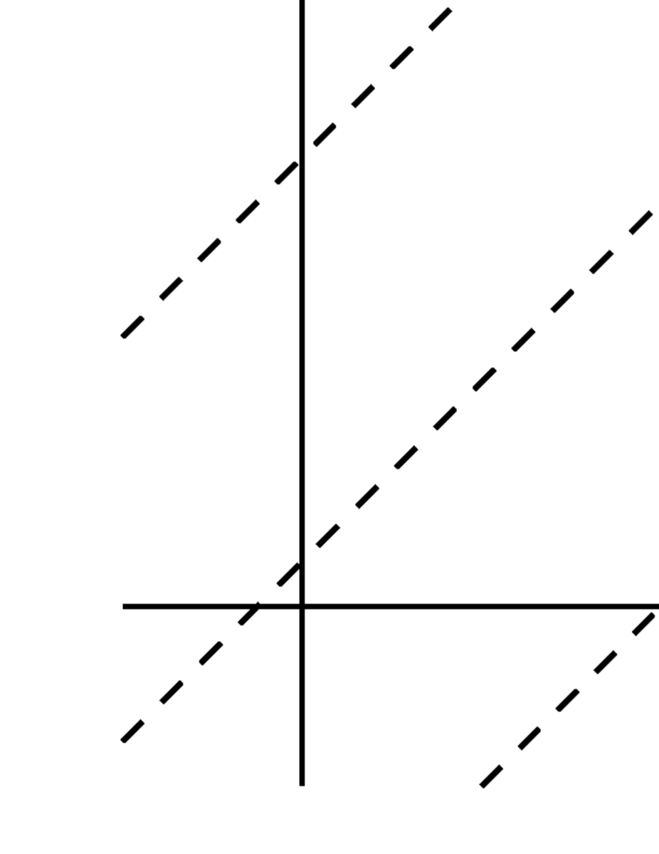
Figure 1: Schematic plot of the two choices of the cutoff $\tau_{\infty}$. On the left panel it is fixed as a constant $\tau_{\infty}=-1/(c_{s}k_{\infty})$ and is the same for every mode. Meanwhile on the right panel it varies for different $k$ in such a way that it corresponds to a fixed length scale, $c_{s}k|\tau_{\infty}|=\gamma_{p}$.

(A) $\tau_{\infty}=-1/(c_{s}k_{\infty})$:

This corresponds to fixing $\tau_{\infty}$ common to all modes. This will be the case when there is a phase transition at $\tau=\tau_{\infty}$ Vilenkin:1982wt . In this case, $-c_{s}k\tau_{\infty}=k/k_{\infty}\gg 1$ and we can think of three simple possibilities that give $k$-independent ${f_{\rm NL}}$:

1. $\varphi_{k}\ll 1$: In this case we find

   $${\cal B}\approx-\frac{1}{2}\frac{k}{k_{\infty}}\varphi_{k}\sinh(2\chi_{k})\approx-\frac{{\cal A}^{2}-1}{4{\cal A}}\frac{k}{k_{\infty}}\varphi_{k}\,.$$ (22)

   Thus, by choosing $\varphi_{k}=\gamma_{c}k_{\infty}/k$, with $\gamma_{c}$ being constant, we can make ${f_{\rm NL}}$ scale-invariant.

2. $2\chi_{k}\ll 1$: Likewise, we find

   $${\cal B}\approx-\frac{1}{2}\frac{k}{k_{\infty}}2\chi_{k}\,\sin\varphi_{k}\,.$$ (23)

   Thus $2\chi_{k}\approx\gamma_{c}k_{\infty}/k$ with a $k$-independent $\varphi_{k}$ works as well. Note that in this case, $\varphi_{k}$ is constant but its value is not constrained, and ${\cal A}\approx 1$ so that the state is very close to the BD vacuum.

3. $\varphi_{k}\ll 1$ and $2\chi_{k}\ll 1$: We have

   $${\cal B}\approx-\frac{1}{2}\frac{k}{k_{\infty}}\varphi_{k}2\chi_{k}\,.$$ (24)

   Thus, choosing $\varphi=p(k_{\infty}/k)^{n}$ and $2\chi_{k}=q(k_{\infty}/k)^{1-n}$ with $p$, $q$ and $0<n<1$ being constant gives ${\cal B}=-pq/2$, so that ${f_{\rm NL}}$ is $k$-independent.

(B) $\tau_{\infty}=-\gamma_{p}/(c_{s}k)$ with $\gamma_{p}\gg 1$:

In this case, the cutoff $\tau_{\infty}$ depends on $k$ in such a way that $-c_{s}k\tau_{\infty}=\gamma_{p}$ is constant. This is the case when the cutoff corresponds to a fixed, very short physical distance. Hence this cutoff may be relevant when we consider possible trans-Planckian effects Shiu:2005si . Again, let us consider three simple possibilities:

1. $\varphi_{k}\ll 1$: We obtain

   $${\cal B}\approx-\frac{\gamma_{p}}{2}\varphi_{k}\sinh(2\chi_{k})\approx-\frac{\gamma_{p}\left({\cal A}^{2}-1\right)}{4{\cal A}}\varphi_{k}\,.$$ (25)

   Thus we require $\varphi_{k}$ to have no $k$-dependence in order to have a scale-invariant ${f_{\rm NL}}$.

2. $2\chi_{k}\ll 1$: In this case ${\cal B}\approx-(\gamma_{p}/2)2\chi_{k}\sin\varphi_{k}$. Thus it is $k$-independent if both $\varphi_{k}$ and $\chi_{k}$ are constant, for an arbitrary value of $\varphi_{k}$.

3. $\varphi_{k}\ll 1$ and $2\chi_{k}\ll 1$: This gives

   $${\cal B}\approx-\frac{\gamma_{p}}{2}\varphi_{k}\,2\chi_{k}\,.$$ (26)

   This is a limiting case of the second case above, and the simplest example is when both $\varphi_{k}$ and $2\chi_{k}$ are $k$-independent.

We note that in all the cases considered above, ${f_{\rm NL}}$ can be large, say ${f_{\rm NL}}\gtrsim 10$, if $c_{s}^{2}\neq 1$ and the constant $\gamma_{c}$ or $\gamma_{p}$ is large.

IV Conclusion

In this article, focusing on single-field slow-roll inflation, we have studied in detail the squeezed limit of the bispectrum when the initial state is a general vacuum. In this case, the standard consistency relation between the spectral index of the power spectrum of the curvature perturbation and the amplitude of the squeezed limit of the bispectrum does not hold. In particular, the squeezed limit of the bispectrum may not be slow-roll suppressed.

Under the assumption that the comoving curvature perturbation is conserved on super-sound-horizon scales, we have derived the general relation between the squeezed limit of the primordial bispectrum, described in terms of the non-linear parameter ${f_{\rm NL}}$ and the power spectrum. We find ${f_{\rm NL}}$ is indeed not slow-roll suppressed. But it depends explicitly on the momentum in general, hence may not be in the local form. We then have discussed the condition for ${f_{\rm NL}}$ to be momentum-independent. We have considered two typical ways to fix the initial state. One is to fix the state at a given time, common to all modes. The other is to fix the state for each mode at a given physical momentum. The former and the latter may be relevant when there was a phase transition, and when discussing trans-Planckian effects, respectively. We have spelled out the conditions for both cases and presented simple examples in which a large, scale-invariant ${f_{\rm NL}}$ is realized.

Naturally it is of great interest to see if these simple examples can be actually realized in any specific models of inflation. Researches in this direction are left for future study.

Acknowledgements

JG is grateful to the Yukawa Institute for Theoretical Physics at Kyoto University for hospitality while this work was under progress. We are grateful to Xingang Chen and Takahiro Tanaka for valuable comments on the first version of the paper. JG acknowledges the Max-Planck-Gesellschaft, the Korea Ministry of Education, Science and Technology, Gyeongsangbuk-Do and Pohang City for the support of the Independent Junior Research Group at the Asia Pacific Center for Theoretical Physics. This work was supported in part by the JSPS Grant-in-Aid for Scientific Research (A) No. 21244033.

References

- (1) A. H. Guth, Phys. Rev. D 23, 347 (1981); K. Sato, Mon. Not. Roy. Astron. Soc. 195, 467 (1981); A. D. Linde, Phys. Lett. B 108, 389 (1982); A. Albrecht and P. J. Steinhardt, Phys. Rev. Lett. 48, 1220 (1982).
- (2) C. L. Bennett, D. Larson, J. L. Weiland, N. Jarosik, G. Hinshaw, N. Odegard, K. M. Smith and R. S. Hill et al., arXiv:1212.5225 [astro-ph.CO].
- (3) [Planck Collaboration], arXiv:astro-ph/0604069.
- (4) For a recent collection of reviews, see e.g. Class. Quant. Grav. 27, “Focus section on non-linear and non-Gaussian cosmological perturbations” (2010); Adv. Astron. 2010, “Testing the Gaussianity and Statistical Isotropy of the Universe” (2010).
- (5) E. Komatsu and D. N. Spergel, Phys. Rev. D 63, 063002 (2001) [astro-ph/0005036].
- (6) J. M. Maldacena, JHEP 0305, 013 (2003) [astro-ph/0210603].
- (7) P. Creminelli and M. Zaldarriaga, JCAP 0410, 006 (2004) [astro-ph/0407059].
- (8) A. Achucarro, J. -O. Gong, G. A. Palma and S. P. Patil, arXiv:1211.5619 [astro-ph.CO].
- (9) J. Ganc and E. Komatsu, JCAP 1012, 009 (2010) [arXiv:1006.5457 [astro-ph.CO]]; S. Renaux-Petel, JCAP 1010, 020 (2010) [arXiv:1008.0260 [astro-ph.CO]].
- (10) M. H. Namjoo, H. Firouzjahi, M. Sasaki and , Europhys. Lett. 101, 39001 (2013) [arXiv:1210.3692 [astro-ph.CO]]; X. Chen, H. Firouzjahi, M. H. Namjoo and M. Sasaki, arXiv:1301.5699 [hep-th].
- (11) X. Chen, M. -x. Huang, S. Kachru and G. Shiu, JCAP 0701, 002 (2007) [hep-th/0605045]; R. Holman and A. J. Tolley, JCAP 0805, 001 (2008) [arXiv:0710.1302 [hep-th]].
- (12) I. Agullo and L. Parker, Phys. Rev. D 83, 063526 (2011) [arXiv:1010.5766 [astro-ph.CO]]; J. Ganc, Phys. Rev. D 84, 063514 (2011) [arXiv:1104.0244 [astro-ph.CO]]; D. Chialva, JCAP 1210, 037 (2012) [arXiv:1108.4203 [astro-ph.CO]]; N. Agarwal, R. Holman, A. J. Tolley and J. Lin, arXiv:1212.1172 [hep-th]. See also S. Kundu, JCAP 1202, 005 (2012) [arXiv:1110.4688 [astro-ph.CO]].
- (13) F. Arroja, A. E. Romano and M. Sasaki, Phys. Rev. D 84, 123503 (2011) [arXiv:1106.5384 [astro-ph.CO]]; F. Arroja and M. Sasaki, JCAP 1208, 012 (2012) [arXiv:1204.6489 [astro-ph.CO]].
- (14) T. Tanaka and Y. Urakawa, JCAP 1105, 014 (2011) [arXiv:1103.1251 [astro-ph.CO]]; T. Tanaka and Y. Urakawa, arXiv:1209.1914 [hep-th].
- (15) J. Garriga and V. F. Mukhanov, Phys. Lett. B 458, 219 (1999) [hep-th/9904176].
- (16) M. Sasaki, Prog. Theor. Phys. 76, 1036 (1986).
- (17) C. T. Byrnes and J. -O. Gong, Phys. Lett. B 718, 718 (2013) [arXiv:1210.1851 [astro-ph.CO]].
- (18) A. Vilenkin and L. H. Ford, Phys. Rev. D 26, 1231 (1982).
- (19) See e.g. G. Shiu, J. Phys. Conf. Ser. 18, 188 (2005) and references therein.