Penetration of a magnetic wall into thin ferromagnetic electrodes of a nano-contact spin valve

Abstract

We theoretically analyzed a magnetic wall confined in a nano-contact spin valve paying special attention to the penetration of the magnetic wall into thin ferromagnetic electrodes. We showed that, compared with the Bloch wall, the penetration of the Néel wall is suppressed by increases of the demagnetization energy. We found the optimal conditions of the radius and height of the nano-contact to maximize the power of the current-induced oscillation of the magnetic wall. We also found that the thermal stability of the Bloch wall increases when the nano-contact’s radius increases or height decreases.

Magnetic walls have attracted much attention as a basic element of nano-spintronics devices such as a racetrack memoryhayashi2008 , spin-wave logic gatesallwood2005 , a read-head for ultra-high-density magnetic recordinggarcia1999 ; imamura2000 ; takagishi2009 , and a spin-torque oscillator (STO)He2007 ; Ono2008 ; franchin2008 ; suzuki2009 ; matsushita09B ; Bisig2009 . The nano-contact spin valve with a geometrically confined magnetic wall shown in Fig. 1 (a) is a nanostructure suitable for the latter two applications, and much effort has been devoted to studying its electric and magnetic propertiesgarcia1999 ; ono1999 ; bruno1999 ; Gorkom:1999 ; imamura2000 ; coey2001 ; chopra2005 ; suzuki2009 . It is widely accepted that a magnetic wall should be created in the nano-contact when the magnetization vectors of the top and bottom electrodes are aligned to be anti-parallel. The magnetic wall in the nano-contact can be categorized into two types: the Bloch wall and the Néel wall. The magnetic moments of the Bloch (Néel) wall rotate along the axis parallel (perpendicular) to the nano-contactmatsushita09A ; matsushita10 ; arai2012 . The read head utilizes the resistance change due to the creation of a magnetic wall, and the STO utilizes the oscillation between the Bloch wall and the Néel wall induced by the applied direct current.

In early experimentsgarcia1999 ; ono1999 ; chopra2005 the break junction of a ferromagnetic wire was employed to realize the nano-contact spin valve, and the corresponding theoretical analysis predicted that the magnetic walls were almost completely confined in the contact region. The point is that the energy required to rotate the magnetic moments in the contact is much less than that in the electrode of the ferromagnetic wire. However, if the thickness of the electrode is as small as the height of the contact, the energy required to rotate the magnetic moments in the electrode becomes so small that the magnetic wall can penetrate into the electrode Molyneux02 ; Jubert05 ; KohnSlastikov06 as shown in Fig 1 (b). Recently the nano-contact spin valve with thin ferromagnetic electrodes Fuke07 has been considered a powerful candidate for 2-5 Tb/in² read sensorstakagishi2010 . Therefore, it is important to analyze the penetration of the magnetic wall into the thin ferromagnetic electrodes of the nano-contact spin valve.

In this paper, we derived analytical expression of a magnetic wall penetrating into the thin ferromagnetic electrodes of a nano-contact spin valve. Based on the derived analytical formula we studied the power of the current-induced oscillation and the thermal stability of the magnetic wall.

The nano-contact spin valve we consider is schematically shown in Fig. 1 (a). To model the anti-parallel configuration of the spin valve, we applied fictitious magnetic fields of magnitude $H$ to the top (bottom) electrode in the positive (negative) $x$-direction. The top and bottom electrodes were assumed to be square plates with width $L$, depth $L$ and thickness $d$. The nano-contact was assumed to be a cylinder with radius $a$ and height $h$. The electrodes and contact were assumed to be made of the same ferromagnetic material. The $z$-axis was taken to be parallel to the nano-contact and the electrodes parallel to the $xy$-plane. The origin of the coordinates was set to be the center of the nano-contact.

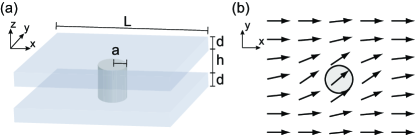
Figure 1: (a) A nano-contact spin valve is schematically shown. (b) A schematic illustration of the penetration of the magnetic wall into the ferromagnetic electrode. The shaded circle represents the area of the nano-contact.

The direction of the magnetization can be expressed by the polar angle $\theta$ and the azimuthal angle $\phi$. The energy in the contact is given by

$$E_{\rm C}=\pi a^{2}\int_{-h/2}^{h/2}dz\,A\left[\left(\frac{\partial\theta}{\partial z}\right)^{2}+\sin^{2}\theta\left(\frac{\partial\phi}{\partial z}\right)^{2}\right],$$ (1)

where $A$ is the exchange stiffness constant. Because the exchange interaction energy is dominant in the nano-contactbruno1999 , we neglected the demagnetization and Zeeman energies.

The energy of the top electrode is given by

$$E_{\rm T}= 2\pi d\int_{a}^{\infty}dr\,r\left[A\left(\dot{\theta}^{2}+\sin^{2}\theta\,\dot{\phi}^{2}\right)\right.$$

$$+\left.\frac{\mu_{0}M_{\rm s}^{2}}{2}\cos^{2}\theta-\mu_{0}M_{\rm s}H\left(\sin\theta\,\cos\phi-1\right)\right],$$ (2)

where $r=\sqrt{x^{2}+y^{2}}$, $\dot{\phi}=\partial\phi/\partial r$, $\dot{\theta}=\partial\theta/\partial r$, $M_{\rm s}$ is the saturation magnetization, and $\mu_{0}$ is the permeability of the vacuum. The first, second and third terms of Eq. (2) represent the exchange interaction energy, demagnetization energy, and Zeeman energy, respectively. The energy of the bottom electrode $E_{\rm B}$ is the same as $E_{\rm T}$. Assuming that the $L$ is much larger than the penetration length of the magnetic wall, the system can be regarded to be rotationally symmetric about the $z$-axis; i. e., the angles $\phi$ and $\theta$ depend only on the radius $r$.

It is worth pointing out that, in the ground state, magnetization in the top electrode $\mbox{\boldmath$m$}_{\rm T}(r)$ and that in the bottom electrode $\mbox{\boldmath$m$}_{\rm B}(r)$ are related as $(-m_{\rm T}^{x},m_{\rm T}^{y},m_{\rm T}^{z})=(m_{\rm B}^{x},m_{\rm B}^{y},m_{\rm B}^{z})$ due to the symmetry of the system. In the following, we calculate the magnetic structure by taking this fact into account.

Let us first consider the Bloch wall, where we assume that $\theta=\pi/2$, $d\theta/dz=0$, and $\dot{\theta}=0$. The energy of the contact is given by

$$E_{\rm C}=\pi a^{2}\int_{-h/2}^{h/2}dz\,A\left(\frac{\partial\phi}{\partial z}\right)^{2}=\frac{2\pi a^{2}A}{h}(\pi-2\phi_{0})^{2}.$$ (3)

To derive the last equation, we have assumed that $\phi|_{z=h/2}=\phi_{0}$ and $\phi|_{z=-h/2}=\pi-\phi_{0}$. We hereafter call $\phi_{0}$ the boundary angle. We have also used the fact that $\phi$ is a linear function of $z$. Note that the corresponding Euler equation is $\partial^{2}\phi/\partial z^{2}=0$. The energy of the top electrode is

$$E_{\rm T}=2\pi d\int_{a}^{\infty}dr\,r\left[A\dot{\phi}^{2}-\mu_{0}M_{\rm s}H\left(\cos\phi-1\right)\right].$$ (4)

The corresponding Euler equation was obtained as

$$\ddot{\phi}+\frac{1}{r}\dot{\phi}-\frac{\mu_{0}M_{\rm s}H}{2A}\sin\phi=0.$$ (5)

The angle $\phi$ at $r=a$ should be consistent with the boundary condition $\phi_{z=h/2}=\phi_{0}$ for the contact and magnetic moments align in the direction of the magnetic field at $r=\infty$. We therefore obtained the boundary conditions $\phi|_{r=a}=\phi_{0}$ and $\phi|_{r=\infty}=0$. In the bottom electrode the boundary conditions should be $\phi|_{r=a}=\pi-\phi_{0}$ and $\phi(\infty)=\pi$. The energy of the electrode, which is a function of $\phi_{0}$, was obtained by substituting the solution of Eq. (5) into Eq. (4) and performing the integral. The boundary angle $\phi_{0}$ was obtained by minimizing the total energy $E_{\rm total}=E_{\rm C}+E_{\rm T}+E_{\rm B}$.

Figure 2: (a) The energies of the contact $E_{\rm c}$, the top and bottom electrodes $E_{\rm T}+E_{\rm B}$, and the total energy are plotted against the boundary angle $\phi_{0}$ by the dotted, dashed, and solid lines, respectively. (b) The function $G(\tilde{a})$ of Eq. (10) is plotted as a function of $\tilde{a}$. (c) The boundary angle $\phi_{0}$ is plotted as a function of the thickness of the electrode $d$. (d) The analytical solution of the angle $\phi$ in the top electrode given by Eqs. (8) and (11) is plotted by the solid line against the distance $r$ from the center of the contact. The result obtained by the Monte Carlo simulation is plotted by the dotted line. The parameters are given in the main text.

We introduce the characteristic lengthMicromagneticBook determined by the competition between the exchange interaction energy and the Zeeman energy as $\ell=\sqrt{2A/\mu_{0}M_{\rm s}H}$ and use the superscript “$\sim$” to indicate the normalized values such as $\tilde{r}=r/\ell$, $\tilde{a}=a/\ell$, $\tilde{d}=d/\ell$, and $\tilde{h}=h/\ell$. Then Eq. (5) is expressed as

$$\ddot{\phi}+\frac{1}{\tilde{r}}\dot{\phi}-\sin\phi=0,$$ (6)

where $\ddot{\phi}=\partial^{2}\phi/\partial{\tilde{r}}^{2}$ and $\dot{\phi}=\partial\phi/\partial{\tilde{r}}$. Assuming that $\phi\lesssim\pi/4$ in the top electrode, the last term of Eq. (6) can be approximated as $\sin\phi\simeq\phi$ and we have

$$\ddot{\phi}+\frac{1}{\tilde{r}}\dot{\phi}-\phi=0.$$ (7)

Equation (7) is the zeroth-order modified Bessel equation whose solutions are the zeroth-order modified Bessel function of the first kind $I_{0}({\tilde{r}})$ and the second kind $K_{0}({\tilde{r}})$. Since $I_{0}({\tilde{r}})$ diverges at the limit of $\tilde{r}\to\infty$, the angle $\phi({\tilde{r}})$ should be expressed as

$$\phi({\tilde{r}})=\phi_{0}\frac{K_{0}({\tilde{r}})}{K_{0}(\tilde{a})}.$$ (8)

Substituting the approximation $\cos\phi\simeq 1-\frac{1}{2}\phi^{2}$ and Eq. (8) into Eq. (4) we have

$$E_{\rm T}=2\pi d\,G(\tilde{a})\,\phi_{0}^{2},$$ (9)

where

$$G(\tilde{a}) =\frac{\tilde{a}K_{1}({\tilde{a}})}{K_{0}({\tilde{a}})}.$$ (10)

Here, $K_{1}({\tilde{r}})$ is the first modified Bessel function of the second kind.

In Fig. 2 (a), we plot the energies $E_{\rm C}$ (dotted-line), $E_{\rm T}+E_{\rm B}$ (dashed-line) and $E_{\rm total}$ (solid-line) as functions of $\phi_{0}$. Here and hereafter we use the following parameters. The saturation magnetization is $M_{\rm s}=1.74\times 10^{6}$ A/m, the exchange stiffness constant $A=20.7$ pJ, the external field $H=7.96\times 10^{4}$ A/m ($1$ kOe), the thickness of the electrodes $d=2$ nm, the height of the contact $h=2$ nm, and the radius of the contact $a=1$ nm. The corresponding characteristic length is $\ell=15.4$ nm. Note that two parameters $a$ and $h$ will be varied in Figs. 2 (c), 3 (a-b) and 4 (a-b). As shown in Fig. 2 (a) $E_{\rm C}$ ($E_{\rm T}+E_{\rm B}$) is a parabolic function of the boundary angle $\phi_{0}$ whose axis of symmetry is located at $\phi_{0}=0$ $(\pi/2)$, and $E_{\rm total}$ takes the minimum value at a certain value of $\phi_{0}$. Setting the first derivative of $E_{\rm total}$ to be zero, we found that the boundary angle of the ground state is

$$\phi_{0}=\frac{\pi}{2}\left[\frac{{\tilde{a}}^{2}}{{\tilde{a}}^{2}+{\tilde{d}}\,{\tilde{h}}\,G(\tilde{a})}\right].$$ (11)

For the nano-contacts with $\tilde{a}\simeq\tilde{h}$, one can easily see that the boundary angle $\phi_{0}$ depends strongly on the value of $\tilde{d}$ because the function $G(\tilde{a})\simeq\tilde{a}$ as shown in Fig. 2 (b). In the limit of $\tilde{d}\to\infty$ the boundary angle $\phi_{0}$ converges to zero, which means that the magnetic wall is perfectly confined in the contact as expected from the discussions in Ref. bruno1999, . The value of $\phi_{0}$ increases with decreasing $\tilde{d}$ and reaches $\pi/2$ at the limit of $\tilde{d}\to 0$. In Fig. 2 (c) we plot the value of $\phi_{0}$ as a function of the thickness of the electrode $d$. If we assume that the thickness of the electrode is the same as the height of the contact; i.e, $d=2$ nm, the boundary angle is as large as $\phi_{0}=37.7\degree$.

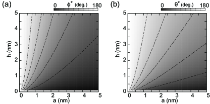
Figure 3: (a) The twist angle of the Bloch wall is plotted as a function of the contact radius $a$ and contact height $h$. The interval of the contours is 30°. (b) The same plot of the Néel wall.

We also performed Monte CarloMonteCarloBook (MC) simulation to confirm the accuracy of the analytical formula we derived. In the MC simulation, the width and depth of the electrode $L$ were set to be $L=100$ nm, which is large enough to eliminate the size dependence. As shown in Fig. 2 (d) the angle $\phi(r)$ obtained by the MC simulation was well reproduced by our analytical formula of Eq. (8) with Eq. (11).

Let us move on to the Néel wall where we assume that the azimuthal angle $\phi=0$, $d\phi/dz=0$, and $\dot{\phi}=0$. We also assume that $-\pi/2\leq\theta\leq\pi/2$. The energy of the contact is given by

$$E_{\rm C}=\pi a^{2}\int_{-h/2}^{h/2}dz\,A\left(\frac{\partial\theta}{\partial z}\right)^{2}=\frac{2\pi a^{2}A}{h}(\pi-2\theta_{0})^{2},$$ (12)

where we have assumed that $\theta|_{z=h/2}=\pi/2-\theta_{0}$ and $\theta|_{z=-h/2}=\theta_{0}-\pi/2$. Note that Eq. (12) is equivalent to Eq. (3). By rewriting $\theta$ in Eq. (2) with $\delta\theta\equiv\pi/2-\theta$ and taking up to the second order of $\delta\theta$, we obtain

$$E_{\rm T}=2\pi d\int_{a}^{\infty}dr\,r\left[A\dot{\delta\theta}^{2}+\frac{\mu_{0}M_{\rm s}H_{\rm eff}}{2}\delta\theta^{2}\right],$$ (13)

where $H_{\rm eff}\equiv H+M_{\rm s}$. The Euler equation for the Néel wall is given by

$$\ddot{\delta\theta}+\frac{1}{r}\dot{\delta\theta}-\frac{\mu_{0}M_{\rm s}H_{\rm eff}}{2A}\delta\theta=0.$$ (14)

The boundary conditions are $\delta\theta|_{r=a}=\theta_{0}$ and $\delta\theta|_{r\to\infty}=0$ in the top electrode, and $\delta\theta|_{r=a}=\pi-\theta_{0}$ and $\delta\theta|_{r\to\infty}=\pi$ in the bottom electrode. Since Eq. (14) takes the same form as Eq. (7) except that $H$ is replaced with $H_{\rm eff}$, we can calculate $\delta\theta$ in a similar way as we calculate the Bloch wall, by replacing the characteristic length $\ell$ with $\ell_{\rm eff}\equiv\sqrt{2A/\mu_{0}M_{\rm s}H_{\rm eff}}$. Assuming the same parameters as in Fig. 2 (a) $\ell_{\rm eff}$ is estimated to be 3.1 nm. The energy of the top electrode $E_{\rm T}$ and the boundary angle $\theta_{0}$ of the ground state of the Néel wall are calculated from Eqs. (9) and (11), respectively, by changing the length for the normalization from $\ell$ to $\ell_{\rm eff}$.

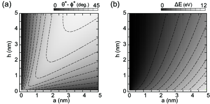
Figure 4: (a) The difference between the twist angles $\theta^{\ast}$ and $\phi^{\ast}$ is plotted against the contact radius $a$ and the contact height $h$. (b) The same plot for the energy difference between the Néel and the Bloch walls.

In order to discuss the difference of the magnetic structures between the Bloch wall and the Néel wall we introduce the twist angles $\phi^{\ast}$ and $\theta^{\ast}$, which are defined as $\phi^{\ast}\equiv\bigl{|}\phi|_{z=h/2}-\phi|_{z=-h/2}\bigr{|}=\pi-2\phi_{0}$ for the Bloch wall and $\theta^{\ast}\equiv\bigl{|}\theta|_{z=h/2}-\theta|_{z=-h/2}\bigr{|}=\pi-2\theta_{0}$ for the Néel wall. As shown in Figs. 3 (a) and (b) $\theta^{\ast}$ is always larger than $\phi^{\ast}$ because the penetration of the Néel wall costs more demagnetization energy in the electrodes compared with that of the Bloch wall. Since the resistance of the magnetic wall is proportional to the twist anglelevy1997 , the conditions for maximizing the power of the current-induced oscillation between the Bloch wall and the Néel wall are the same as those for the difference between $\theta^{\ast}$ and $\phi^{\ast}$. In Fig. 4 (a) we plot the difference $\theta^{\ast}-\phi^{\ast}$ as a function of $a$ and $h$. One can see that the optimum conditions for maximizing the power of the STO based on the nano-contact spin valve are approximately given by $a\sim h$.

Figure 4 (b) shows the difference between the energies of the Néel wall and the Bloch wall defined as $\Delta E\equiv E_{\mbox{\scriptsize N{\'{e}}el}}-E_{\rm Bloch}$ as a function of $a$ and $h$. The energy difference $\Delta E$, and therefore the thermal stability of the Bloch wall, increases with increasing $a$ or decreasing $h$. In the plotted region ($0<a,h\leq 5$nm) the Bloch wall is the ground state and the Néel wall the excited state, contrary to the results of the perfectly confined magnetic wall shown in Ref. coey2001, . The energy difference $\Delta E$ for the perfectly confined magnetic wall originates from the demagnetization energy in the contact that we neglected. Following Ref. coey2001, we can estimate $\Delta E\simeq$0.16 eV for a perfectly confined magnetic wall with $a=$1 nm and $h=$2 nm. On the other hand, for the the nano-contact spin valve with thin ferromagnetic electrodes, the main contribution to $\Delta E$ is from the demagnetization energy in the electrodes. The estimated value of $\Delta E$ is about 3.0 eV, which is about 19 times larger than that of the perfectly confined magnetic wall.

In summary, we theoretically studied the effects on a magnetic structure of a nano-contact spin valve with thin ferromagnetic electrodes. We derived analytical formulas for the magnetic configurations of the Bloch wall and the Néel wall, and the corresponding energies. We showed that, compared with the Bloch wall, the penetration of the Néel wall into the electrodes is suppressed by the increase of the demagnetization energy. We found the optimum conditions for maximizing the power of the STO based on the nano-contact spin valve are given by $a\sim h$. We also found that the thermal stability of the magnetic wall increases as the nano-contact’s radius increases or height decreases.

- (1) M. Hayashi, L. Thomas, R. Moriya, C. Rettner, and S. S. P. Parkin, Science 320, 209 (2008).
- (2) D. A. Allwood, G. Xiong, C. C. Faulkner, D. Atkinson, D. Petit, and R. P. Cowburn, Science 309, 1688 (2005).
- (3) M. M. N. García and Y.-W. Zhao, Phys. Rev. Lett. 82, 2923 (1999).
- (4) H. Imamura, N. Kobayashi, S. Takahashi, and S. Maekawa, Phys. Rev. Lett. 84, 1003 (2000).
- (5) M. Takagishi, H. N. Fuke, S. Hashimoto, H. Iwasaki, S. Kawasaki, R. Shiozaki, and M. Sahashi, J. Appl. Phys. 105, 07B725 (2009).
- (6) J. He and S. Zhang, Appl. Phys. Lett. 90, 142508 (2007).
- (7) T. Ono and Y. Nakatani, Appl. Phys. Express 1 061301 (2008).
- (8) M. Franchin, T. Fischbacher, G. Bordignon, P. de Groot,and H. Fangohr, Phys. Rev. B 78, 054447 (2008).
- (9) K. Matsushita, J. Sato and H. Imamura, J. Phys. Soc. Jpn. 78, 093801 (2009).
- (10) A. Bisig, L. Heyne, O. Boulle, and M. Klaui, Appl. Phys. Lett. 95, 162504 (2009).
- (11) H. Suzuki, H. Endo, T. Nakamura, T. Tanaka, M. Doi, S. Hashimoto, H. N. Fuke, M. Takagishi, H. Iwasaki, and M. Sahashi, J. Appl. Phys. 105, 07D124 (2009).
- (12) T. Ono, Y. Ooka, H. Miyajima, and Y. Otani, Appl. Phys. Lett. 75, 1622 (1999).
- (13) P. Bruno, Phys. Rev. Lett. 83, 2425 (1999).
- (14) R. P. van Gorkom, J. Caro, S. J. C. H. Theeuwen, K. P. Wellock, N. N. Gribov, and S. Radelaar, Appl. Phys. Lett. 74, 422 (1999).
- (15) J. M. D. Coey, L. Berger, and Y. Labaye, Phys. Rev. B 64, 020407(R) (2001).
- (16) H. D. Chopra, M. R. Sullivan, J. N. Armstrong, and S. Z. Hua, Nature Materials 4, 832 (2005).
- (17) K. Matsushita, J. Sato and H. Imamura, J. Appl. Phys. 105, 07D525 (2009).
- (18) K. Matsushita, J. Sato, H. Imamura, and M. Sasaki, J. Phys. Soc. Jpn. 79, 093801 (2010).
- (19) H. Arai, H. Tsukahara, and H. Imamura, Appl. Phys. Lett. 101, 092405 (2012).
- (20) V. A. Molyneux, V. V. Osipov, and E. V. Ponizovskaya, Phys. Rev. B 65, 184425 (2002).
- (21) P.-O. Jubert and R. Allenspach, J. Magn. Magn. Mater. 290-291, 758 (2005).
- (22) R. V. Kohn and V. V. Slastikov, Calc. Var. Part. Diff. Equ. 28, 33 (2006).
- (23) H. N. Fuke, S. Hashimoto, M. Takagishi, H. Iwasaki, S. Kawasaki, K. Miyake, and M. Sahashi, IEEE Trans. Magn. 43, 2848 (2007).
- (24) M. Takagishi, K. Yamada, H. Iwasaki, H. N. Fuke, and S. Hashimoto, IEEE Trans. Magn. 46, 2086 (2010).
- (25) H. Kronmüller and M. Fähnle, Micromagnetism and the Microstructure of Ferromagnetic Solids (Cambridge University Press, Cambridge, 2003) Chap. 13.
- (26) D. P. Landau and K. Binder, A Guide to Monte Carlo Simulations in Statistical Physics (3rd ed.) (Cambridge University Press, Cambridge, 2009).
- (27) P. M. Levy and S. Zhang, Phys. Rev. Lett. 79, 5110 (1997).