Multiple stellar populations in Magellanic Cloud clusters. II.       Evidence also in the young NGC 1844?

We use HST observations to study the LMC’s young cluster NGC 1844. We estimate the fraction and the mass-ratio distribution of photometric binaries and report that the main sequence presents an intrinsic breadth which can not be explained in terms of photometric errors only, and is unlikely due to differential reddening. We attempt some interpretation of this feature, including stellar rotation, binary stars, and the presence of multiple stellar populations with different age, metallicity, helium, or C+N+O abundance. Although we exclude age, helium, and C+N+O variations to be responsible of the main-sequence spread none of the other interpretations is conclusive.

1 Introduction

High-accuracy photometry, mainly with Hubble Space Telescope (HST) is revealing multiple sequences in the color-magnitude diagrams (CMDs) of a growing number of Galactic globular clusters (GGCs, e.g.  Bedin et al. 2004, Anderson 1997, Piotto et al. 2007, Milone et al. 2008, Lee et al. 2009). Spectroscopy also shows that multiple stellar populations are a common feature among old GCs (e.g.  Kraft et al. 1992, Yong et al. 2008, Marino et al. 2008, Carretta et al. 2009).

The presence of multiple stellar populations seems not to be an exclusive property of old stellar systems, as again, thanks to HST observations, also the intermediate-age clusters (IACs) in the Magellanic Clouds (MCs) have been found to host multiple stellar populations (Bertelli et al. 2003, Baume et al. 2007, Mackey & Broby Nielsen 2007, Mackey et al. 2008, Glatt et al. 2008a,b, Goudfrooij et al. 2009, 2011).

It is now confirmed that over 70% (probably a lower limit set by the quality of the available data) of the $\sim$1-3 Gyr old MCs’ clusters studied so far reveal some broadening of their sequences (Milone et al. 2009, hereafter Paper I), pointing to stellar populations with inhomogeneity in the chemistry, age, rotation, other physical properties of their stars (see Keller et al. 2011 for a discussion)

It is worthwhile to extend the study to stellar clusters younger than $\sim$300 Myr to investigate if the processes that generate broadened or multiple stellar sequences in the CMDs of GGCs and MCs’ clusters are similar in nature or not, and to put constraints on when, after the cluster birth, these processes set in.

In this work we begin an investigation of young clusters searching for the presence of multiple stellar populations among their stars. The target of the present study is NGC 1844, for which a summary of its main parameters is given in Table 1. To our knowledge, the present study is the first attempt to extend the study multiple populations to a $\sim$150 Myr old cluster.

2 Observations, Measurements, and Selections

This work is based on coordinated parallel observations obtained with the wide field channel (WFC) of the Advanced Camera for Surveys (ACS) at the focus of the Hubble Space Telescope (HST) under program GO-12219 (PI: Milone). The primary target of the program, entitled “Multiple stellar generations in the Large Magellanic Cloud Star Cluster NGC 1846”, was indeed, NGC 1846, for which Wide Field Camera 3 observations were collected. At the phaseII-stage of GO-12219 we realized that the two clusters NGC 1846 and NGC 1844 were almost exactly separated by the angular distance between the two far-most corners of the field of views of the two cameras: ACS/WFC and the UV and visual (UVIS) channel of WFC3, on the HST focal plane. We, therefore, decided to point and orient HST in a way to collect images for both clusters simultaneously, in one shot (see Fig. 1).

This work is focused on NGC 1844, for which data were collected between 16 and 17 of April 2011, and consist of 7$\times$900s images in filter F475W, and 1$\times$326s $+$ 4$\times$340s $+$ in F814W. A companion work will deal with NGC 1846. All images were dithered by whole and fractional pixels, as described in Anderson & King (2000). Before performing measurements of the sources’ positions and fluxes, we applied our recently developed pixel-based correction for imperfect Charge Transfer Efficiency (CTE, Anderson & Bedin, 2010). Figure 2 shows a trichromatic stacked image of the studied ACS/WFC field, after removal of cosmic rays and most of the artefacts. As it can be seen, this choice of pointing allows for a proper estimate of the LMC field contamination. We will use this field to statistically correct the NGC 1844’s CMD from field contamination.

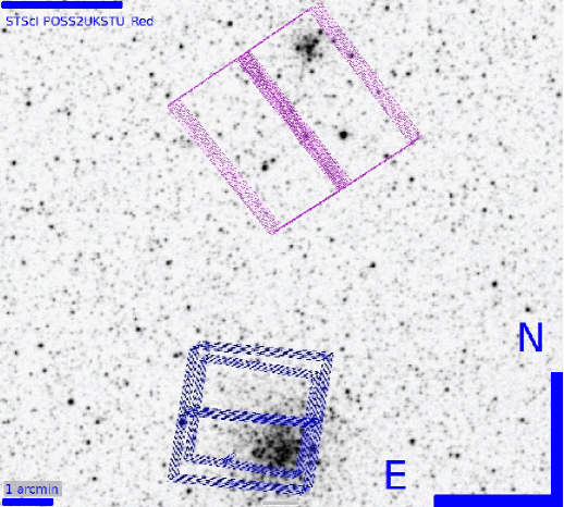
Figure 1: (Online Material). Layout of the simultaneous observations of NGC 1846 (bottom) and NGC 1844 (top) (from HST’s Astronomer’s Proposal Tool). The individual ACS/WFC images are shown in magenta, and those of WFC3 (in both UVIS and NIR channels) in blue. Note the intrinsic different size of the two clusters, as they are almost at the same distance.

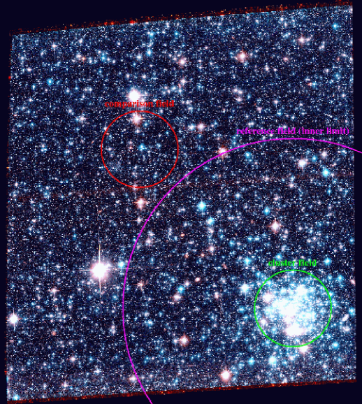
Figure 2: (Online Material). Stacked trichromatic image of the studied NGC 1844’s ACS/WFC-field. The green circle indicates the region considered cluster (cluster field), while the circle in red is an equal-size random region shown for comparison (comparison field). The circle in magenta indicates the inner limit of the portion of the ACS/WFC field used as reference to statistically remove the LMC’s field contamination from the CMD of NGC 1844.

Photometry and relative positions were obtained with the software tools described by Anderson et al. (2008). The photometry was calibrated into the WFC/ACS Vega-mag system following the procedures given in Bedin et al. (2005b), and using encircled energy and zero points given by Sirianni et al. (2005). We will use for these calibrated magnitudes the symbols $m_{\rm F475W}$ and $m_{\rm F814W}$.

Artificial-star (AS) tests were performed using the procedures described by Anderson et al. (2008). In the present program we chose them to cover the magnitude range $20<m_{\rm F475W}\leq 30$, with colors that placed them on the main sequence (MS). Completeness has been calculated as in Paper I (see Sect. 2.2) and accounts for both the crowding conditions and stellar luminosity. Figure 3 shows the completeness contours in the radius versus magnitude plane.

Stars that saturate are treated as described in Sect. 8.1 in Anderson et al. (2008). Collecting photo-electrons along the bleeding columns allows us to measure magnitudes of saturated stars up $\sim$3.5 mag above saturation (i.e. , up to $m_{\rm{F814W}}\sim$20, and $m_{\rm{F475W}}\sim$20), with errors of only a few percent (Gilliland 2004). We used $\sim$80 sources in the 2mass catalog, to register our absolute astrometry. The calibrated catalog, and an astrometrized image is released to the community as part of this work.

The analysis we present here requires high-precision photometry, so we selected a high-quality sample of stars that (1) have a good fit to the point-spread function, (2) are relatively isolated, (3) and have small astrometric and photometric errors (see Paper I, Section 2.1 for a detailed description of this procedure).

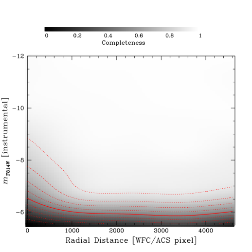
Figure 3: (Online Material). Completeness contours in the radial-distance versus $m_{\rm F814W}$ magnitude plane. The completeness is proportional to the gray level as indicated by the scale on the top. Continuous lines correspond to completeness level of 0.50. Dotted lines indicate differences of completeness of 0.10.

Table 1: Parameters for NGC 1844 derived in this work.

$(m-M)_{\rm F814W}$	$E(m_{\rm F475W}-m_{\rm F814W})$	age(Myr)	Z	[Fe/H]	core radius (arcsec)	tidal radius (arcsec)	concentration
18.52	0.15	150	0.01	$-$0.6	22	57	0.4

3 The Color-Magnitude Diagrams

Figure 4 shows the CMDs for all the detected sources in the studied field. The objects highlighted in red are those within 450 ACS/WFC pixels (i.e. $\sim$22^′′, assuming a 49.7248 mas ACS/WFC-pixel scale, from van der Marel et al. 2007) from the assumed cluster’s center at (R.A.;DEC)=(05:07:30.462;$-$67:19:27.79) [or in pixel-coordinates: (4400;1780)].

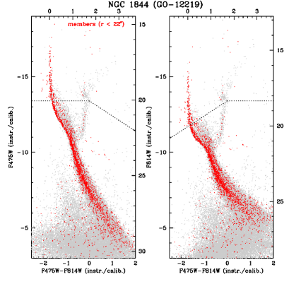
Figure 4: CMDs for all the sources in the field (grey points). The objects within 22 arcsec from the assumed cluster center are shown as red dots. A dashed line indicates the set in of saturations.

A more careful inspection at the MS reveal some color structure. Figure 5, shows a quantitative analysis of this color-structure. On the left panel we present the same $m_{\rm F814W}$ versus $m_{\rm F475W}-m_{\rm F814W}$ CMD of Fig. 4, with indicated the fiducial line of the main MS component and the loci (dashed line) occupied by the corresponding equal-mass binaries. A box indicates the region of the MS where this color-structure is most evident. The top-right panel shows a blow-up of this box, without the fiducial-line for clearness. The bottom-right panels show respectively, the “rectified MS” (obtained by subtracting from the color of each star the color of the fiducial at the corresponding magnitude) and the histogram of this distribution.

It is clear that the color distribution of the MS of NGC 1844 in this range of magnitudes has an anomalous red-ward skew. We will see in the following that a very peculiar binary mass-ratio distribution is required to reproduce the observations (cfr Sect. 3.2).

In the upper-left panel of Fig. 6 we plot the Hess diagram for this portion of the CMD for all objects within 22.3 arcsec from the assumed cluster center (hereafter cluster field). The upper-middle panel shows the Hess diagram for a field with radial distance from the cluster center R$>$100 arcsec, where no cluster members are expected (see Fig. 2); we will refer to this as the reference field.

To statistically remove the contamination of field stars in the Hess diagram of stars in the cluster field, we have compared the Hess diagrams of the cluster and the reference field. For each interval of color and magnitude used to make these two Hess diagrams, we have calculated the number of cluster stars as $N_{\rm CL}=N_{\rm CF}-f_{\rm AREA}N_{\rm RF}$, where $N_{\rm CF}$ and $N_{\rm RF}$ is the measured number of stars, corrected for completeness, in the cluster and reference field, respectively, and $f_{\rm AREA}$ is the ratio between the area of the cluster field and the area of the reference field. The Hess diagram of the cluster after that field stars have been statistically removed is shown the the upper-right panel. This plot demonstrates that the MS broadening cannot be explained by field contamination.

In the lower-left panel of Fig. 6 we show again a blow-up of a the same portion of the CMD for stars in the cluster field. In order to provide, a discrete-point example of the field contamination in the CMD of the cluster, the bottom-middle panel shows the CMD for stars within an area covering the same amount of sky of the cluster field. This was taken in an area away from NGC 1844, within the reference field (see Fig. 2, outside the circle in magenta); we will refer to this as comparison field (in red in Fig. 2) and will not be used for the quantitative analysis in this paper.

Finally, lower-right panel shows the same CMD for the artificial stars added along the fiducial lines, after an additional broadening to account for the tendency of artificial star tests to underestimate photometric errors (see discussion in Paper I). The direct comparison of the two CMDs reveals an internal breadth of the MS of $\sim$0.1 in color, which cannot be explained either from field contamination or photometric errors.

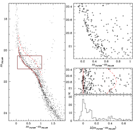
Figure 5: On the left, the $m_{\rm F814W}$ vs. $m_{\rm F475W}-m_{\rm F814W}$ CMD for stars in the cluster field. Saturated stars are colored gray. The solid and the dashed lines are the MS ridge line and the locus of equal-mass binaries, respectively. On the Right, we show a zoom-in of the same CMD in the region highlighted by the box, i.e. where the MS broadening is most clearly visible (upper panel), the verticalized CMD (middle panel), and the color histogram distribution (lower panel). [See text].

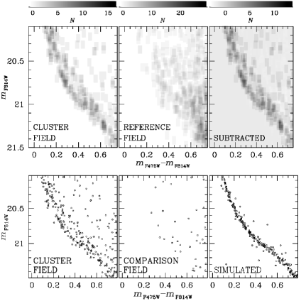
Figure 6: Top-panels: Hess diagrams around the anomalous MS-breadth of NGC 1844 for the selected cluster field, the reference field, and for the area-normalized difference of the two. Bottom-panels: CMD focused on the same region for the point sources measured in the cluster field, those measured in a comparison field, and for the photometry of ASs placed along the MS fiducial line.

3.1 Simulation of Binaries

A visual inspection of the CMD of NGC 1844 reveals a large number of photometric binaries on the red side of the MS (Fig. 4). In this section we investigate whether these objects can account for the observed MS broadening.

To do this we started by deriving the fraction of MS-MS binaries with mass ratio $q>$0.4 by assuming that the MS broadening is due to binaries alone. Briefly, we divided the CMD in two parts: a region “A” populated by single stars and the binaries with a primary with 20.3$<m_{\rm F814W}<$21.3 (the shadowed area in the upper panels of Fig. 7) and a region “B” which is the portion of A containing the binaries with $q>$0.4 (the darker area in the upper panels of Fig. 7). The reddest line is the locus of the equal-mass binaries red-shifted by four $\sigma$ (where $\sigma$ is the error estimated as in Paper I). The bluest line is the MS fiducial moved by four $\sigma$ to the blue. The locus of the CMD of binaries with a given mass-ratio has been determined by using the mass-luminosity relation of Pietrinferni et al. (2004).

The fraction of binaries with $q>0.4$ is calculated as in Eq. 1 in Milone et al. (2012) (repeated here for convenience):

$$f_{\rm bin}^{\rm q>0.4}=\frac{N_{\rm REAL}^{\rm B}-N_{\rm FIELD}^{\rm B}}{N_{\rm REAL}^{\rm A}-N_{\rm FIELD}^{\rm A}}-\frac{N_{\rm ART}^{\rm B}}{N_{\rm ART}^{\rm A}},$$ (1)

where $N_{\rm REAL}^{\rm A,(B)}$ is the number of stars in the cluster field (corrected for completeness) observed in the CMD’s region A (B); $N_{\rm ART}^{\rm A,(B)}$, and $N_{\rm FIELD}^{\rm A,(B)}$ are the corresponding numbers of artificial stars and of stars observed in the reference field and normalized to area of the cluster field. We find $f_{\rm bin}^{\rm q>0.4}$=0.39$\pm$0.05. We repeated the same procedure for the fraction of binaries with $q>$0.6 and $q>$0.8 and derived the fraction of binaries in three intervals of size $\Delta q=$0.2 in the interval $0.4<q<1$.

In the magnitude interval 20.3$<m_{\rm F814W}<$21.3, the fractions of binaries with $0.8<q<1$ and $0.6<q<0.8$ are similar (0.10$\pm$0.03 and 0.07$\pm$0.03 respectively) but we need a $23\pm 5$% of binaries with $0.4<q<0.6$ to account for the MS broadening. Results are plotted in Fig. 8.

To further investigate the influence of binaries on the MS morphology, we analyzed the CMD region with 21.3$<m_{\rm F814W}<$22.3 where there is no evidence for an intrinsic color spread. Results are illustrated in the lower panels of Fig. 7. By using the procedure described above, we find $f_{\rm bin}^{\rm q>0.4}$=0.30$\pm$0.05 and in this case each of the three analyzed mass-ratio contains about the 10% of the binaries.

For completeness we extended the study of binary to fainter magnitudes. The binary fractions in the magnitude intervals 22.3$<m_{\rm F814W}<$23.3 and 23.3$<m_{\rm F814W}<$24.3 are listed in Table 2 and are plotted against $q$ in Fig. 8. Due to the rise of the photometric error, the color distance of binaries with $q<0.6$ from the MS fiducial is smaller than three times $\sigma$, making it not possible to distinguish them from single MS stars. In these cases, we limited our study to binaries with mass ratio $q>0.6$.

In addition, we repeated the same analysis described above, by using the $m_{\rm F475W}$ versus $m_{\rm F475W}-m_{\rm F814W}$ CMD. We analyzed four F475W intervals that corresponds to the four F814W bins previously defined, and obtained similar results, as listed in Table 2. We enphasize that, due to the relatively small number of binaries and the statistical approach used to subtract the background, any conclusion on the flatness of the q-distribution could be an over-interpretation of the data.

In summary, our investigation is not conclusive; the MS broadening could be due to binaries, but this hypothesis would imply an ad hoc mass-ratio distribution for the photometric binaries, with a large fraction of them concentrated in the interval of magnitude 20.3$<m_{\rm F814W}<$21.3 and mass ratio $0.4<q<0.6$.

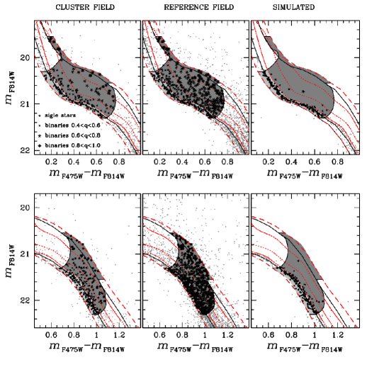
Figure 7: CMD of stars in the cluster field (left), the comparison field (middle), and simulated stars (right). The black continuous lines are the MS fiducials and the locus of equal-mass binaries, while the loci of binaries with mass ratio $q=$0.4, 0.6, and 0.8 are represented with dotted red lines (see text for more details). Upper and lower panels show the setup used to measure the fraction of binaries in the intervals 20.3$<m_{\rm F814W}<$21.3 and 21.3$<m_{\rm F814W}<$22.3 respectively.

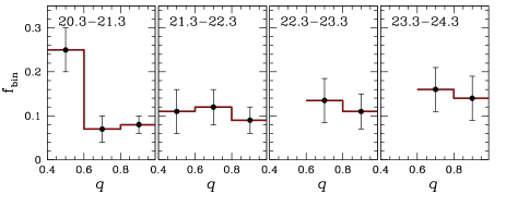
Figure 8: Histogram distributions of the fraction of binaries as a function of the mass ratio, in four $m_{\rm F814W}$ intervals indicated in each panel.

Table 2: Fraction of binaries for different luminosity and mass-ratio intervals.

Luminosity bin		$f_{\rm bin}$
F814W	$0.4<q<0.6$	$0.6<q<0.8$	$0.8<q<1.0$
20.3-21.3	0.25$\pm$0.05	0.07$\pm$0.03	0.08$\pm$0.02
21.3-22.3	0.11$\pm$0.05	0.12$\pm$0.05	0.08$\pm$0.04
22.3-23.3	—	0.13$\pm$0.05	0.11$\pm$0.04
23.3-24.3	—	0.16$\pm$0.05	0.14$\pm$0.05
F475W	$0.4<q<0.6$	$0.6<q<0.8$	$0.8<q<1.0$
20.46-21.99	0.23$\pm$0.05	0.05$\pm$0.03	0.10$\pm$0.03
21.99-23.31	0.08$\pm$0.05	0.11$\pm$0.04	0.09$\pm$0.03
23.31-24.57	—	0.13$\pm$0.05	0.15$\pm$0.04
24.57-25.93	—	0.17$\pm$0.05	0.17$\pm$0.05

3.2 Differential reddening

The extinction due to Galactic interstellar medium (ISM) in the direction of NGC 1844 is $E(B-V)=0.05$ (Schlegel, Finkbeiner, & Davis 1998) and such a small reddening is usually uniform over a scale of few arcsec. As an example, in Paper I we have shown that the CMD of NGC 1846, a cluster in the LMC located about 5 arcmin S-W from NGC 1844, reveals a very narrow RGB and a well defined red clump thus suggesting that any reddening variation in the area should be very small [$E(B-V)<0.007$]. The color difference between stars on the blue and red side of the MS of NGC 1844 is typically $\Delta\sim 0.07$ mag and is too large to be explained in terms of reddening variations only, as these variations would be larger than the average reddening itself [$E(B-V)\sim 0.05$ mag].

To investigate whether differential reddening is responsible for the MS broadening of NGC 1844 we applied the procedure illustrated in Fig. 9. We selected in the cluster field’s CMD two groups of bona-fide blue-MS and red-MS stars that we color-coded in blue and red respectively in the upper-left panel. The same colors are used consistently in the other panels.

The upper-right panel shows that the spatial distribution of blue- and red-MS stars is the same (within the statistical uncertainties). We have then divided the cluster field in four parts (quadrants) and plotted in the lower panels the corresponding CMDs. The numbers of blue-MS and red-MS stars are labeled in the lower-left corner of each CMD-panel, and give the same ratio of red-to-blue stars within 1 $\sigma$. However, we note that the small number of stars prevents us from a more significant analysis of the inference of reddening variations on shorter angular scales.

The present analysis suggests that differential reddening produced by Milky Way ISM is unlikely the responsible for the MS broadening of NGC 1844. However we can not exclude that differential absorption due to the possible presence of intra-cluster nebulosity could generate this effect.

The cumulative radial distributions of blue-MS and red-MS stars are shown in Fig. 10. The Kolmogorov-Smirnov statistic shows that in random samplings from the same distribution a difference this large would occur 89% of the time, which is very reasonable for the hypothesis that the two MSs have the same distribution.

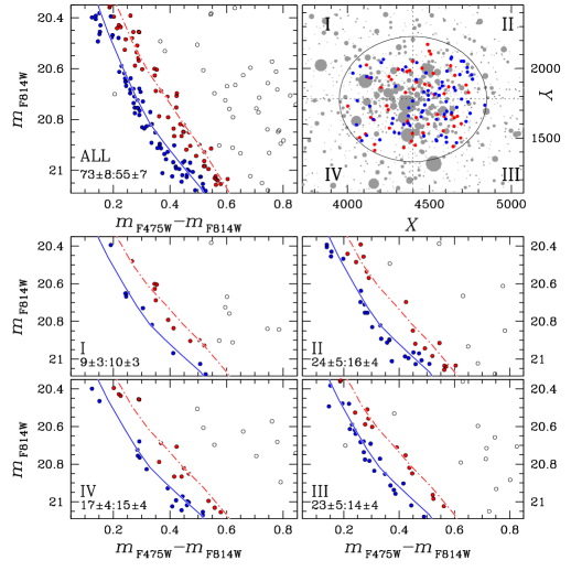
Figure 9: (Online Material). Upper-left panel: CMD of stars in the cluster field zoomed-in around the region where the MS broadening is more evident. Stars on the blue and the red MS side are color-coded in blue and red respectively, the continuous and the dashed-dotted lines are the fiducial of the two MS regions drawn by hand. Upper-right panel: Spatial distribution of blue- and red-MS stars. Lower panels: CMDs for stars in the four quadrants defined in the upper-right panel.

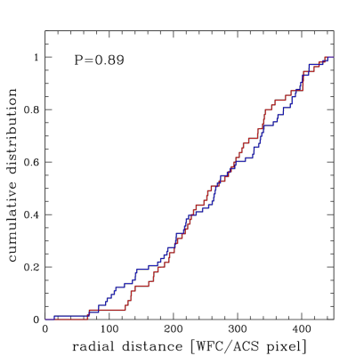
Figure 10: (Online Material). Cumulative radial distribution of blue-MS (blue line) and red-MS (red line).

4 Comparison with Theory

To understand the physical reasons of the MS-broadening discussed in the previous sections, we have performed qualitative comparisons of observations with theoretical predictions as taken from the BaSTI archive. In doing this we employed both the $\alpha$-enhanced and CNO-enhanced stellar models (Pietrinferni et al. 2004, 2006, 2009) specifically transformed into the ACS/WFC photometric Vega-mag system (Bedin et al. 2005). The adopted evolutionary stellar models account for the occurrence of core convective overshoot during the central H-burning stage by adopting the numerical assumptions and formalism discussed in Pietrinferni et al. (2004).

These comparisons are in the form of best fits to the observed CMD of NGC 1844 with isochrones calculated under different scenarios, which are discussed in the following subsections where we investigate the effect of CNO, metallicity, and helium- variation as well as the effect of stellar rotation.

4.1 CNO

The top-left panel of Fig. 11 shows that an $\alpha$-enhanced isochrone for Z$=$0.01 and age of 150 Myr (solid line) reproduces finely the morphology of the bulk of the MS as well as the cluster TO brightness. [Hereafter —unless otherwise specified— we adopt $(m-M)_{\rm F814W}=18.52$  mag and $E(m_{\rm F475W}-m_{\rm F814W})=A_{\rm F475W}-A_{\rm F814W}=0.15$.]

The same figure also shows that an isochrone based on stellar models with a factor of $\sim$2 enhancement in the CNO-element sum is able to match the red boundary of the MS locus. So, the observed MS-broadening could be due to a spread in the (C$+$N$+$O) among stars in NGC 1844.

However, the brighter portion of the CNO-enhanced isochrones crosses a region of the CMD where no stars are observed. So, only an ad hoc mass function for the (C$+$N$+$O)-enhanced component could reconcile this scenario with the observations.

4.2 Metallicity

As an alternative scenario, we explored the possibility that the MS-broadening could be due to an intrinsic metallicity spread: the top-right panel of Fig. 11 shows that the color spread of the MS locus in NGC 1844 is confined within the theoretical predictions provided by two isochrones with metallicity Z=0.01 and 0.015. This means that a metallicity spread of the order of 0.15-0.20 dex could account for the observed MS’s broadening. Most importantly, this scenario is able to provide a better match than the previous one to the observed star distribution in the brightest portion of the CMD, i.e. $18.5<m_{\rm F814W}<20.5$.

4.3 Helium

It is commonly accepted that the MS broadening (or split) observed in many GGCs hosting multi-populations (such as $\omega$ Cen, NGC 2808, NGC 6752, and 47 Tuc) is mainly due to a significant helium-abundance enhancement. However, as we will see, this scenario seems not to work to explain the MS broadening of NGC 1844. The bottom-left panel of Fig. 11 shows the comparison between the empirical data and selected isochrones for a fixed metallicity (Z$=$0.008) and two different assumptions about the initial He content (Y$=$0.256 and Y$=$0.300). In this case we had to adopt a shorter distance modulus of $(m-M)_{\rm F814W}=18.40$ mag. The He-enhanced isochrone matches the hotter boundary of the MS locus corresponding to the bulk of the cluster stellar population, while the isochrone corresponding to the ‘canonical’ He abundance is not able to properly match the cooler edge of the MS locus. The agreement could improve by using a larger He enhancement ($Y\approx 0.33$) but at the expense of an even smaller distance modulus; a choice not supported by current best estimates of the LMC distance (e.g. Tammann, Sandage & Reindl, 2008, and references therein).

4.4 Rotation

Lastly, we explore another physical process that could help in explaining the observed MS broadening of NGC 1844: rotation of stars. Indeed, this process is able to affect both the evolutionary lifetimes and the morphology of the evolutionary tracks (Maeder & Meynet 2000). Briefly, the centrifugal acceleration reduces the effective gravity resulting in cooler and slightly less luminous stars. However, rotation also induces internal mixing processes, which can have the opposite effect, i.e. leading to more luminous and hotter stars. Which of these contrasting effects dominate depends on the initial mass, rotational velocity and chemical composition.

It has been suggested that the presence of fast rotators among MS stars could be the cause of the occurrence of multiple MS turn-offs in several intermediate age clusters of the MCs (Bastian & De Mink 2009). Although Girardi et al. (2011) compared isochrones from models with and without rotation with the observed CMDs and excluded this possibility, stellar rotation is a good candidate to explain the broadening of the MS locus in cluster as young as NGC 1844.

In fact, in the intermediate-mass regime —the one relevant in the present investigation (i.e. 150-Myr-young clusters)— and for stars still in the core H-burning stage, the dominant effect induced by rotation is the reduction of both the effective temperature and luminosity with respect to not-rotating stellar structures. Therefore, the existence of a spread in the rotational rate among the stars of NGC 1844 could help to explain the MS-breadth.

A detailed investigation of stellar rotation is beyond the aims of the present work, therefore, to quantify the effect of stellar rotation on our isochrones, we have adopted a simplified approximation.

In the bottom-right panel of Fig. 11 we compare a selected portion of the NGC 1844’s CMD (where the MS broadening is more evident) with two isochrones. The first one (solid, blue line) is the same isochrone as adopted in the top-left panel of Fig. 11 ($\alpha$-enhanced, Z=0.01). The second one (dashed, red line) is the same isochrone after modifying its effective temperature and luminosity to take into account the effect of rotation. In order to account for rotation we followed the detailed recipes given in Bastian & De Mink (2009). According to their formalism, we adopted the following values for the relevant parameters: $a=0.18$, $b=0.5$ and $\omega=0.5$. Although, we are aware that this approach is extremely simplified, the data shown in the quoted figure reveal that the presence of a spread in the rotational rates can help in explaining the MS broadening.

Whatever the reason of the intrinsic breadth of the MS of NGC 1844, we have demonstrated that it is significantly broader than what can be expected from photometric errors, and therefore real. Further investigation, from both a theoretical and an observational point of view, should be pursued.

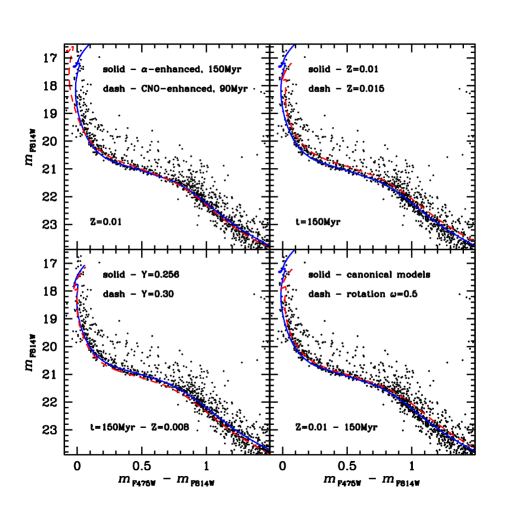
Figure 11: (Top-Left Panel): Comparison between the observed CMD of NGC1844 and suitable theoretical isochrones for an age of 150 Myr and 90 Myr for two different assumptions about the heavy element mixtures: an $\alpha$-enhanced mixture ([$\alpha$/Fe]=$+0.4$, solid blue line) and a CNO-enhanced one (dashed, red line), both with the same iron content [Fe/H]=$-0.6$. In this comparison we assumed $(m-M)_{\rm F814W}=18.52$ and $E(m_{\rm F475W}-m_{\rm F814W})=0.15$ for both isochrones. (Top-Right): In this case the two isochrones have the same $\alpha$-enhanced mixture but different metallicities, namely Z=0.01 and Z=0.015. (Bottom-Left): In this case the two isochrones have the same metallicity, Z=0.008, but two different initial He abundances. In this last case we adopted $(m-M)_{\rm F814W}=18.40$. (Bottom-Right): Comparison between the NGC1844’s MS and the same isochrone ($\alpha$-enhanced, 150 Myr, Z=0.01) adopted in the Top-Left panel (solid, blue line). To investigate the impact of stellar rotation, we also show the same isochrone modified according to Bastian & De Mink (2009) recipes to take into account the effect of rotation according (dashed, red line). [See text for more details].

- (1) Anderson, A. J. 1997, Ph.D. Thesis, Univ. of California, Berkeley
- (2) Anderson, J., & King, I. R. 2000, PASP, 112, 1360
- (3) Anderson, J., & Bedin, L. R. 2010, PASP, 122, 1035
- (4) Anderson, J., et al. 2008, AJ, 135, 2055
- (5) Bastian, N., & De Mink, S.E. 2009, MNRAS, 398, L11
- (6) Baume, G., Carraro, G., Costa, E., Méndez, R. A., & Girardi, L. 2007, MNRAS, 375, 1077
- (7) Bedin, L. R., Piotto, G., & Anderson, J., et al., 2004, ApJ, 605, L125
- (8) Bedin, L. R., Cassisi, S., Castelli, F., Piotto, G., Anderson, J., Salaris, M., Momany, Y., & Pietrinferni, A. 2005b, MNRAS, 357, 1038
- (9) Bedin, L. R., et al. 2008, ApJ, 679, L29
- (10) Bertelli, G., Nasi, E., Girardi, L., et al. 2003, AJ, 125, 770
- (11) Carretta, E., Bragaglia, A., Gratton, R. G., et al. 2009, A&A, 505, 117
- (12) D’Ercole, A., D’Antona, F., Carini, R., Vesperino, E., & Ventura, P. 2012, MNRAS, 423, 1521
- (13) Gilliland, R. 2004, ACS Instrument Science Report 2004-01
- (14) Girardi, L., Eggenberger, P., & Miglio, A. 2011 MNRAS, 412, L103
- (15) Glatt, K., Grebel, E. K., Sabbi, E., et al. 2008a, AJ, 136, 1703
- (16) Glatt, K., Grebel, E. K., Sabbi, E., et al. 2008b, AJ, 135, 1106
- (17) Goudfrooij, P., Puzia, T. H., Kozhurina-Platais, V., & Chandar, R. 2009, AJ, 137, 4988
- (18) Goudfrooij, P., Puzia, T. H., Kozhurina-Platais, V., & Chandar, R. 2011, ApJ, 737, 3
- (19) Keller, S. C., Mackey, A. D., & Da Costa, G. S. 2011, ApJ, 731, 22
- (20) Kraft, R. P., Sneden, C., Langer, G. E., & Prosser, C. F. 1992, AJ, 104, 645
- (21) King, I. 1962, AJ, 67, 471
- (22) Maeder, A., & Meynet, G. 2000, ARA&A, 38, 143
- (23) Mackey, A. D., & Broby Nielsen, P. 2007, MNRAS, 379, 151
- (24) Mackey, A. D., Broby Nielsen, P., Ferguson, M. N., & Richardson, J. C. 2008, ApJ, 681, L17
- (25) Lee, J.-W., Kang, Y.-W., Lee, J., & Lee, Y.-W. 2009, Nature, 462, 480
- (26) Marino, A. F., Villanova, S., Piotto, G., et al. 2008, A&A, 490, 625
- (27) Milone, A. P., Piotto, G., Bedin, L., R., et al. 2012, A&A, 540, 16
- (28) Milone, A. P., Bedin, L. R., & Piotto, G. et al. 2008, ApJ, 673, 241
- (29) Milone, A. P., Bedin, L. R., Piotto, G., & Anderson, J. 2009, A&A, 497, 755
- (30) Pietrinferni, A., Cassisi, S., Salaris, M., & Castelli, F. 2004, ApJ, 612, 168
- (31) Pietrinferni, A., Cassisi, S., Salaris, M., & Castelli, F. 2006, ApJ, 642, 797
- (32) Pietrinferni, A., Cassisi, S., Salaris, M., Percival, S., & Ferguson, J. W. 2009, ApJ, 697, 275
- (33) Piotto, G., Bedin, L. R., & Anderson, J. et al. 2007, ApJ, 661, L53
- (34) Piotto, G. 2009, IAUS, 258, 233
- (35) Tammann, G.A., Sandage, A., & Reindl, B. 2008, ApJ, 679, 52
- (36) Schlegel, D. J., Finkbeiner, D. P., Davis, M. 1998, ApJ, 500, 525
- (37) Sirianni, M., et al. 2005, PASP, 117, 1049
- (38) Yong, D., Grundahl, F., Johnson, J. A., & Asplund, M. 2008, ApJ, 684, 1159
- (39) van der Marel, R. P. 2003, Instrument Science Report ACS 2003-10, 10