A Herschel^⋆ and APEX Census of the Reddest Sources in Orion: Searching for the Youngest Protostars^⋆⋆

Abstract

We perform a census of the reddest, and potentially youngest, protostars in the Orion molecular clouds using data obtained with the PACS instrument onboard the Herschel Space Observatory and the LABOCA and SABOCA instruments on APEX as part of the Herschel Orion Protostar Survey (HOPS). A total of 55 new protostar candidates are detected at 70 µm and 160 µm that are either too faint ($m_{24}>7$ mag) to be reliably classified as protostars or undetected in the Spitzer/MIPS 24 µm band. We find that the 11 reddest protostar candidates with log $\lambda F_{\lambda}70/\lambda F_{\lambda}24>1.65$ are free of contamination and can thus be reliably explained as protostars. The remaining 44 sources have less extreme 70/24 colors, fainter 70 µm fluxes, and higher levels of contamination. Taking the previously known sample of Spitzer protostars and the new sample together, we find 18 sources that have log $\lambda F_{\lambda}70/\lambda F_{\lambda}24>1.65$; we name these sources ”PACS Bright Red sources”, or PBRs. Our analysis reveals that the PBRs sample is composed of Class 0 like sources characterized by very red SEDs (T_bol $<$ 45 K) and large values of sub–millimeter fluxes (L_smm/L${}_{\rm bol}>0.6\%$). Modified black–body fits to the SEDs provide lower limits to the envelope masses of 0.2 M_⊙ to 2 M_⊙ and luminosities of 0.7 L_⊙ to 10 L_⊙. Based on these properties, and a comparison of the SEDs with radiative transfer models of protostars, we conclude that the PBRs are most likely extreme Class 0 objects distinguished by higher than typical envelope densities and hence, high mass infall rates.

1. Introduction

The onset of the star formation process is broadly characterized by a dense collapsing cloud envelope surrounding the nascent protostar. The dense cloud or protostellar envelope is opaque to radiation shortward of about $\sim\,$10 µm and most of the radiation from these sources is reprocessed and emitted in the far–infrared (FIR). Furthermore, bipolar outflows from the protostar and disk carve out envelope cavities that enable a fraction of the protostellar luminosity to escape in the form of scattered light emission, predominantly at wavelengths shortward of $\sim\,$10 µm.

The earliest phase of protostellar evolution, the Class 0 phase (André et al., 1993), is thought to be short compared to the Class I phase (Lada, 1987), with combined Class 0 and Class I lifetimes of $\sim\,$0.5 Myr (Evans et al., 2009); these estimates assume a constant star formation rate and a typical age for Class II objects (pre–main sequence stars with disks) of 2 Myr. At the onset of collapse and immediately before the Class 0 phase, protostars may go through a brief first hydrostatic core (FHSC) phase where the forming protostellar object becomes opaque to its own radiation for the first time (Larson, 1969). The FHSC are expected to be very low–luminosity and deeply embedded. A population of very low luminosity protostars (VeLLOs) were also recently identified by Spitzer (e.g., Dunham et al., 2008; Bourke et al., 2006), defined to have model–estimated internal source luminosities of less than 0.1 $L_{\sun}$. VeLLOs, however, appear more evolved than FHSCs with features consistent with Class 0 and I protostars. Furthermore, while several FHSC candidates have been identified recently (e.g., see Enoch et al., 2010; Chen et al., 2010; Pineda et al., 2011; Pezzuto et al., 2012), it has proven observationally difficult to distinguish such sources from the young Class 0 protostellar phase. It is therefore currently difficult to identify the very earliest phases of the formation of a protostar.

Before the launch of Spitzer and the advent of extremely sensitive mid–infrared surveys, conventional wisdom held that a Class 0 protostar should not be detectable at wavelengths shortward of 10 µm due to the envelope opacity (Williams & Cieza, 2011). Outflows, however, can carve out cavities in the protostellar envelopes at a very early age and are expected to widen with evolution (Arce & Sargent, 2006). Indeed, recent simulations have shown that even the extremely young FHSC sources may be capable of driving outflows (Commerçon et al., 2012; Price et al., 2012). Regardless of evolutionary state, the outflow cavities enable near– to mid–infrared light from the protostar and disk to escape and scatter off dust grains in the cavity or on the cavity walls. This phenomenon has been well–known for Class I sources (Kenyon et al., 1993; Padgett et al., 1999), but Class 0 protostars were only well–detected in the mid–infrared with Spitzer (Noriega-Crespo et al., 2004; Jørgensen et al., 2007; Stutz et al., 2008). The scattered light from Class 0 protostars is often brightest at wavelengths $\sim\,$3.6 µm or 4.5 µm due to the dense envelope obscuration at shorter wavelengths (e.g., Whitney et al., 2003a; Tobin et al., 2007).

The combination of results from recent space–based and ground–based surveys have resulted in well–sampled spectral energy distributions from the near–infrared to the (sub)millimeter for large samples of protostellar objects (e.g., Hatchell et al., 2007; Enoch et al., 2009; Launhardt et al., 2010; Fischer et al., 2010; Launhardt et al., 2012). These SEDs are dominated by scattered light between $\sim\,$1 µm and 10 µm, optically thick thermal dust emission from $\sim\,$10 to $\sim\,$160 µm, and optically thin dust emission at wavelengths longward of $\sim\,$160 µm. Radiative transfer models of protostellar collapse have become increasingly important to interpret these data since these can account for the varying temperature and density profiles in the envelopes surrounding the protostar (e.g., Whitney et al., 2003a, b).

The large number of free model parameters — such as the combination of outflow cavities, rotationally flattened envelopes (Ulrich, 1976; Cassen & Moosman, 1981; Terebey et al., 1984), and varying viewing angles — can however make the best–fit SED model parameters highly degenerate (e.g., Whitney et al., 2003a). For example, sources viewed at nearly edge–on orientations can be substantially more obscured than sources at the same evolutionary state viewed from a less extreme vantage point. Thus, standard diagnostics such as bolometric temperature or mid–infrared spectral index can yield vastly different results depending on the source inclination (e.g., Dunham et al., 2010). Radiative transfer models can help break some of these degeneracies but ambiguities can remain as to whether a source has a very dense envelope or if it is simply viewed edge–on.

While much has been learned about the Class 0 phase from observations and modeling, there are relatively few Class 0 objects present in nearby star–forming clouds and globules (Evans et al., 2009) compared to the numbers of Class I and Class II sources. One of the principal goals of recent star formation surveys has been to understand the evolution of protostellar sources. Young & Evans (2005) generated models for the smooth luminosity evolution of protostellar objects that will become 0.3 $\hbox{M}_{\odot}$  1 $\hbox{M}_{\odot}$ and 3 $\hbox{M}_{\odot}$ stars. These models, however, over predict the luminosities of most protostars located in nearby star–forming regions, a fact that is taken as evidence for episodic accretion (Kenyon & Hartmann, 1990; Evans et al., 2009; Dunham et al., 2010). However, Offner & McKee (2011) show that the observed luminosity functions of protostars can be explained through a dependence of the mass accretion rate on the instantaneous and final mass of the protostar. The low resolutions and sensitivities of previous FIR instrumentation have made the detection of protostars in more distant and richer star–forming regions difficult and subject to substantial confusion. Thus, studies of protostellar evolution have been limited to combining all known Class 0 protostars from the nearby regions into a single analysis (e.g., Myers et al., 1998; Evans et al., 2009) to achieve a more robust sample size.

The advent of the Herschel Space Observatory (Pilbratt et al., 2010) has tremendously improved resolution and sensitivity to FIR radiation, where protostars emit the bulk of their energy. These improvements enable the study of protostellar populations to be extended to more distant, richer regions of star formation that have more statistically significant samples of protostars in the Class 0 and I phases (e.g., Ragan et al., 2012). The Herschel Orion Protostar Survey (HOPS) is a Herschel Open Time Key Programme (OTKP) (e.g., Stanke et al., 2010; Fischer et al., 2010; Ali et al., 2010; Manoj et al., 2012) targeting $\sim\,$300 of the Spitzer identified Orion protostars with PACS (Poglitsch et al., 2010) 70 µm and 160 µm photometry and PACS spectroscopy (53 µm to 200 µm; Manoj et al., 2012) for a subset of 30 protostars. Orion is the richest star–forming region within 500 pc of the Sun (Megeath et al., 2012), at a distance of $\sim\,$420 pc (average value; Menten et al., 2007; Hirota et al., 2007; Sandstrom et al., 2007). The large sample of protostars in Orion enables studies of protostellar evolution to be carried out for a single star forming complex where all protostars lie at nearly the same distance with a statistically significant sample, comparable to or larger than all the nearby regions combined. The large sample may also enable short timescale phenomena (e.g., Fischer et al., 2012) to be detected such as brief periods of high envelope infall rate in the earliest phases of star formation. Even with the increased numbers of protostars in Orion, however, it is unclear if we would expect to detect FHSCs given the faintness of these sources and short lifetimes of less than 10 kyr (Commerçon et al., 2012).

The PACS imaging of the HOPS program has the potential to identify protostars that were not detected by Spitzer due to a combination of opacity of the envelope and/or confusion with nearby sources. Indeed, the PACS 70 µm band of Herschel is ideal for detecting such protostars, with the highest angular resolution, limiting the blending of sources. Also, the lower opacity relative to MIPS 24 µm allows the reprocessed warm inner envelope radiation to escape. Finally, and most importantly, a 70 µm point source is strong evidence for an embedded protostar because external heating cannot raise temperatures high enough to emit at this wavelength. Thus, some cores in sub–millimeter surveys that were previously identified as starless may in reality be protostellar.

Using Herschel, we have serendipitously identified a sample of 70 µm point sources that were not identified in the previous Spitzer protostar sample (Megeath et al., 2012). Furthermore, we have identified a subset of these that have the reddest 70 µm to 24 µm colors of all protostars in the combined Orion sample. These sources may have the densest envelopes and are possibly the youngest detected Orion protostars and we name them “PACS Bright Red sources” or PBRs.

We will describe the methodology of identifying these sources and classify them as either being protostellar, extragalactic contamination, or spurious detections coincident with extended emission. We will discuss the observations and data reduction in § 2, the source finding and classification methods in § 3, the observed properties of the new sources in § 4, the PBRs in § 5, the comparison of the cold PBRs to models in § 6, some relevant model degeneracies in § 7, and, finally, our results in § 8. Throughout this work, all positions are given in the J2000 system.

2. Observations, Data Reduction, and Photometry

In this work, we present Herschel scan map observations of a sub–set of the HOPS fields containing candidate protostars. In addition, we present a subset of our APEX LABOCA and SABOCA observations of these fields. A summary of the HOPS Herschel PACS survey observations is presented in Tables 1 and 2. Here we discuss the observations, data processing, and photometry extraction.

2.1. Herschel PACS

The PACS data were acquired simultaneously at 70 µm and 160 µm over 5$\arcmin\times 5\arcmin$ or 8$\arcmin\times 8\arcmin$ field sizes. The field sizes and centers were chosen to maximize observing efficiency by allowing each field to include as many of the target Spitzer–selected protostars (Megeath et al., 2012) as possible while minimizing redundant coverage. The observations were acquired at medium scan speed (20$\arcsec$ sec^-1), and are composed of two orthogonal scans with homogeneous coverage.

The PACS data were reduced using the Herschel Interactive Processing Environment (HIPE) version 8.0 build 248 and 9.0 build 215. We used a custom built pipeline to process data from their raw form (the so–called Level 0 data) to fully calibrated time lines (Level 1) just prior to the map–making step. Our pipeline uses the same processing steps as described by Poglitsch et al. (2010) but also include the following additions and modifications. First, we used a spatial redundancy based algorithm to identify and mask cosmic ray hits. Second, we mitigated instrument cross–talk artifacts by masking (flagging as unusable) detector array columns affected by cross–talk noise. This technique is effective but at the expense of loss of signal from the affected detector array columns. Third, we used the ”FM6” version of the instrument responsivity, which has a direct bearing on the absolute calibration of the final mosaics.

The Level 1 data were processed with “Scanamorphos” (Roussel, 2012) version 14.0. The final maps were produced using the galactic option and included the turn–around (non–zero acceleration) data. The final map pixel scales used in this work are 1.0$\arcsec$/pix at 70 µm and 2.0$\arcsec$/pix at 160 µm.

The photometry was performed in the following fashion. We first derived customized aperture corrections to the 70 µm and 160 µm data using the Herschel Science Center (HSC) provided observations of Vesta (to be discussed in more detail in Fischer et al., in preparation). At 70 µm, we used radii of sizes $9.6\arcsec$, $9.6\arcsec$, and $19.2\arcsec$, for the aperture and sky annuli respectively. For these parameters we derived an aperture correction of $0.7331$, where the measured flux in the aperture is divided by this correction to obtain a total point–source flux. At 160 µm, we used aperture radii of $12.8\arcsec$, $12.8\arcsec$, and $25.6\arcsec$, for the aperture and sky annuli respectively. Similarly, we derived an aperture correction of $0.6602$. The encircled energy fractions provided by the photApertureCorrectionPointSource task in HIPE do not account for the effect of applying an inner sky annulus that is close to the size of the source aperture and small compare to the PSF. Our apertures therefore account for 3–4% of the source flux that is removed. Furthermore, our adopted aperture sizes are smaller than the PACS instrument team recommendation but were chosen to minimize contribution from nebulosity (extended, non point–like emission) often surrounding the protostars in Orion. Given the complex structure in the images and at times crowded fields, our aperture photometry may suffer from blending and contamination. The photometric errors include a 10% systematic error floor added in quadrature to the standard photometric uncertainties. These errors represent systematic uncertainties in our photometry and aperture correction, as well as the overall calibration uncertainty of PACS. We note that the reported HSC point-source calibration uncertainties for PACS are $\sim 3$% at 70 µm and $\sim 5$% at 160 µm, and were derived from isolated photometric standards. Therefore, our final uncertainties are conservative.

We include the 100 µm Gould Belt Survey (GBS; e.g., André et al., 2010; Könyves et al., 2010; Men’shchikov et al., 2010, see also Schneider et al., in preparation, for Orion B, and Roy et al., in preparation, and Polychroni et al., in preparation, for Orion A) data of Orion in this work for the PBRs analysis. Given the sparsely covered SEDs of our sources, these data provide important information regarding the shape of the thermal SED of cold envelope sources. These data were acquired using the medium scan speed (20$\arcsec$ sec^-1) and cover an area much larger than the HOPS fields. These data were processed in a similar way to the HOPS processing described above. Following the above 70 µm and 160 µm analysis, we used aperture radii of sizes $9.6\arcsec$, $9.6\arcsec$, and $19.2\arcsec$, for the aperture and sky annuli respectively. For these parameters, we derived an aperture correction of $0.6944$. As with the 70 µm and 160 µm data, we also assume a conservative 10% systematic error floor.

2.2. APEX SABOCA and LABOCA

We obtained sub–millimeter (smm) continuum maps using the LABOCA and SABOCA bolometer arrays on the APEX telescope. LABOCA (Siringo et al., 2009) is a $\sim\!$250 bolometer array operating at 870 µm, with a spatial resolution of $\sim\!19\arcsec$ at FWHM. We used a combination of spiral and straight on–the–fly scans to recover extended emission. Data reduction was done with the BOA software (Schuller et al., 2012) following standard procedures, including iterative source modeling. SABOCA (Siringo et al., 2010) is a 37 bolometer array operating at 350 µm, with a resolution of $\sim\!7.3\arcsec$ FWHM. The observing and data reduction procedures were similar to those used for LABOCA. For both cameras, observations were carried out between 2009 November and 2012 June, and are still ongoing to complete our Submillimeter Orion Survey. Conditions were generally fair over the course of our observing campaign. The observations will be summarized in more detail by Stanke et al. 2013, in preparation.

The beam sizes of the final reduced maps are $7.34\arcsec$ and $19.0\arcsec$ FWHM for the SABOCA and LABOCA observations, respectively. The photometry was extracted in the same way for both wavelengths. When possible, if there was a strong source detection, we re-centered using the 70 µm catalog source coordinates. Given the contributions of flux due to surrounding cold material, such as filaments and other extended envelope structure, it is likely that a single photometric measure can suffer from large systematic effects. We have measured source fluxes in three ways:
1. We measured the source peak flux per beam.
2. We measured source flux over an aperture with radius equal to the FWHM at the corresponding wavelength (r = $7.34\arcsec$ and $19.0\arcsec$ at 350 and 870 µm, respectively), using a sky annulus with inner and outer radii equal to $[1.5,2.0]\times$FWHM, corresponding to $11.0\arcsec$ and $14.7\arcsec$ at 350 µm, and $28.5\arcsec$ and $38.0\arcsec$ at 870 µm.
3. We measured the flux over the same aperture size as the previous method without any sky subtraction. In the case that a source was not strongly detected and we were not able to re–center, the 70 µm catalog source coordinates was used, along with method 3, and the photometric point was flagged as an upper limit. By re–centering whenever possible, we accounted for possible pointing offsets between data–sets, which can be significant. The calibration error dominated the error budget for well detected sources; we therefore adopted a flux error equal to 20% and 40% of the measured flux for LABOCA and SABOCA respectively. The photometric fluxes are presented in Table 5.

2.3. Spitzer IRAC and MIPS

The IRAC and MIPS imaging and photometry presented here are taken from the 9 degree² survey of the Orion A and B cloud obtained during the cryogenic Spitzer mission. The data analysis, extraction of the IRAC 3.6 µm, 4.5 µm, 5.8 µm, and 8 µm and MIPS 24 µm photometry, and the compilation of a point source catalog containing the combined 2MASS, IRAC and MIPS photometry are described in Megeath et al. (2012); also see Kryukova et al. (2012) for a detailed description of the MIPS 24 µm photometry. In total, 298405 point sources were detected in at least one of the Spitzer bands, and 8021 sources were detected at 24 µm with uncertainties $\leq 0.25$ mag. The Spitzer images used in this work are taken from the mosaics generated from the Orion Survey data using Cluster Grinder for the IRAC data (Gutermuth et al., 2009) and the MIPS instrument team’s Data Analysis Tool for the 24 µm data (Gordon et al., 2005). The MIPS data are saturated toward the Orion Nebula and parts in the NGC2024 region; we exclude these saturated regions from our analysis.

The identification of protostars with the Spitzer data was based primarily on the presence of a flat or rising spectral energy distributions between 4.5 $\mu$m and 24 $\mu$m (Kryukova et al., 2012; Megeath et al., 2012). In addition, Megeath et al. identified objects which have point source detections only at 24 $\mu$m but which also showed other indicators of protostellar nature such as the presence of jets in the IRAC bands. To minimize contamination from galaxies, the Spitzer–identified protostars were required to have 24 $\mu$m magnitudes brighter than $7$th magnitude; fainter than 7 magnitudes, the number of background galaxies begins to dominate over the number of embedded sources (Kryukova et al., 2012). Given the imposed 24 $\mu$m magnitude threshold, the faintest and reddest protostars may not be included in the Spitzer sample. In total, the Megeath et al. (2012) catalog contains 488 protostars. Of these, 428 are classified as bona fide protostars, 50 are faint candidate protostars, and 10 are red candidate protostars. The faint candidate protostars are sources with 24 µm magnitudes higher than 7.0. The red protostars are sources that are only detected as a point source at 24 µm and are thus not classifiable. Due to their location within high extinction regions and/or association with jets or compact scattered light nebulae in the IRAC bands, , they have been included in the catalog. (Indeed, this last category was added to the Megeath et al. catalog after the Herschel data revealed that a relatively large number of such sources would likely be confirmed as protostars.) In addition, the Megeath et al. catalog identified 2992 objects as pre–main sequence stars with disks. In what follows, we use the protostar catalog of 488 Spitzer sources to catalog previously identified sources in the HOPS images.

In contrast to the full Megeath et al. catalog, the HOPS protostar sample represents a sub–set of that catalog. The HOPS sample is not a complete representation of the Megeath et al. catalog because the HOPS survey targeted a smaller area then the Spitzer survey and required an extrapolated 70 µm flux that would be detectable with PACS. However, the HOPS catalog represents our best pre–Herschel knowledge of the protostellar content within the HOPS fields. The HOPS sample is therefore the best one against which to bench–mark and compare the new Herschel protostellar candidates. The HOPS sample constitutes $\sim\,300$ previously identified Spitzer protostars all having Herschel PACS 70 µm detections. Of these, $\sim\,250$ HOPS sources have PACS 160 µm detections. This sample will be analyzed in detail in Fischer et al., in preparation.

In contrast to the full Megeath et al. catalog, the HOPS protostar sample are those protostars specifically targeted by the HOPS program. The majority of the HOPS sample consists of Spitzer–identified protostars with 24 µm detections; hence, protostars in regions that are saturated in the 24 µm images of Orion, namely the brightest regions of the Orion Nebula and NGC2024, are not included. These protostars were also required to have a predicted 70 µm flux $>$ 20 mJy as extrapolated from their 3 µm to 24 µm SEDs. In addition, protostar candidates with only 24 µm detections were included if there was independent information of their protostellar nature. The HOPS sample represents the best pre–Herschel catalog of protostars that were expected to be detected with Herschel/PACS and were not found in bright nebulous regions. There are $\sim\,$300 protostars in the HOPS catalog which have been detected at 70 µm and $\sim\,$250 protostars detected at 160 um. The uncertainty in there absolute number of protostars is due to the ongoing process of eliminating contamination from the sample.

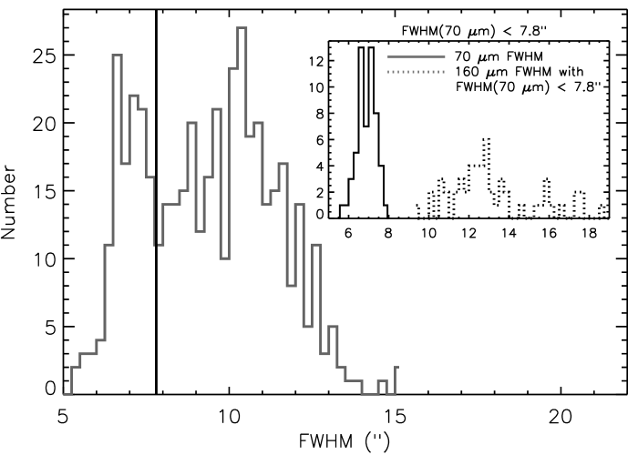
Figure 1.— Frequency of 70 µm FWHM values for all sources detected in our HOPS images that have not been previously identified in the Spitzer catalog. The black line shows our adopted 7.8$\arcsec$ FWHM threshold, above which we reject all sources. Inset: Same as above for the subset of sources with both FWHM(70 µm) $<$ 7.8$\arcsec$ and 160 µm detections (see § 3). The dotted histogram indicates the 160 µm FWHM distribution.

3. Identification of new candidate Herschel protostars

To find protostars which were not reliably identified with Spitzer, we must first isolate a sample of sources that are detected in the PACS 70 µm band but are either fainter than 7.0 magnitudes or undetected in MIPS 24 µm waveband. To identify such sources in each HOPS field we first generate a 70 µm source catalog using the PhotVis tool (Gutermuth et al., 2008). The PhotVis tool uses a sunken Gaussian filtering to extract sources that are of order the size of the Gaussian FWHM, an input parameter. We choose this parameter to be the size of the 70 µm PSF FWHM, or 5$\arcsec$. PhotVis also requires a SNR threshold as input; we adopt a low value of 7 to balance the recovery of as many candidate sources as possible while still rejecting noise spikes.

Furthermore, we must reject unreliable sources near the edges of maps where the lower coverage causes elevated noise levels. The Scanamorphos scan map image cubes include a weight map for each field. Within Scanamorphos, the weight map is computed over the same projection as the sky map, and is defined as one over the variance in the white noise (Roussel, 2012). Each weight map is then normalized by the average map value (Roussel, 2012). We find that for the HOPS data–set, weight map values of $\sim\!$20 are confined to the outer higher noise edges of our scan maps. We therefore use the weight maps to reject edge sources from the catalog at this phase of the analysis. We accomplish this by requiring that the mean value of the weight map in a $9\times 9$ pixel area centered on the candidate source have a value of at least 20. For reference, all HOPS 70 µm scan maps have weight map values greater than 60 over most of the map areas.

The resulting preliminary source catalog includes all sources in the 70 µm images, i.e., previously identified Spitzer sources, new candidate protostars, nebulosity, and other undesirable features and artifacts in the images. We then cross–correlate this PACS 70 µm preliminary catalog with the existing Spitzer catalog to eliminate all previously identified protostars in each field that are brighter than the previously adopted 24 µm cutoff of 7 mag (Megeath et al., 2012). Therefore our sample includes by definition only sources that are faint or undetected in the previous Spitzer catalog.

To identify previous source detections, we require that a source be matched to within a positional offset of 8$\arcsec$ when cross–correlated with the Spitzer catalog. This threshold is conservatively large compared to the Spitzer astrometry and is meant to encompass two main sources of astrometric error. First, it is possible that the absolute coordinates of a source may shift as function of wavelength (although this effect is expected to be relatively small) since different wavelengths may trace different material near the protostars. Second, the Herschel pointing accuracy, which is of order $\sim\,2\arcsec$ ($1\sigma)$, dominates the positional accuracy for most sources when comparing the Spitzer catalog source coordinates to the Herschel 70 µm coordinates. To match coordinates robustly, we therefore adopt a conservatively large 8$\arcsec$ threshold. We find that inspection of the matched sources by eye shows that this threshold works well and provides a low rate of mismatched or duplicate sources.

Our final goal is to obtain a sample of previously unidentified and uncharacterized Herschel protostar candidates. These sources should be characterized by a point–like appearance at 70 µm. Therefore, after rejecting all Spitzer protostars as described above, we next apply a simple FWHM (or apparent size) filter to the remaining 70 µm sources. The distribution of 70 µm azimuthally averaged FWHM values is shown in Figure 1 as the solid black histogram. We find a clear peak in the distribution at low FWHM values, indicating a population of point–like sources. Based on this distribution, we adopt a FWHM threshold of 7.8$\arcsec$, meant to select 70 µm point–sources. We find 127 sources that fulfill the criteria listed here: 85 of these have 24 µm detections while 42 do not.

In a further step, we then require that all 70 µm sources also have a 160 µm detection and not upper limits. The 70 µm FWHM distribution of this sub–set of sources is shown in the inset of Figure 1 along with the corresponding 160 µm FWHM distribution. Our final sample consists of 55 candidate Herschel protostars with both 70 µm and 160 µm detections. Of these, 34 have Spitzer 24 µm detections fainter than 7.0 magnitudes and 21 do not have any 24 µm detection.

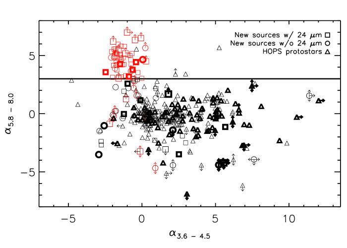
Figure 2.— IRAC color indices $\alpha_{3.6-4.5}$ and $\alpha_{5.8-8.0}$ for sources detected in at least one IRAC band. The Herschel protostar candidate sample is shown as squares (sources with 24 µm detections) and circles (sources without 24 µm detections), while the HOPS protostar sample is shown as triangles. Thick bold points are sources with robust 870 µm detections. Candidate protostars with $\alpha_{5.8-8.0}>3.0$ or upper limits consistent with this threshold are flagged as possible extragalactic contamination and highlighted in red. Note that some candidate protostars have both $\alpha_{5.8-8.0}>3.0$ and a robust 870 µm detection; these sources are not considered extragalactic contamination.

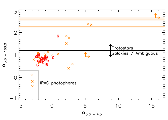
Figure 3.— IRAC and PACS 160 µm color indices $\alpha_{3.6-4.5}$ and $\alpha_{3.6-160}$ for the candidate protostar sample. Sources previously characterized as extragalactic based on their $\alpha_{5.8-8.0}>3$ index (or limit) are indicated in red with a “G”. Sources with $\alpha_{5.8-8.0}<3$ are indicated in orange. The orange lines indicate the lower limits of $\alpha_{3.6-160}$ for sources with no IRAC detections. Sources with $\alpha_{3.6-160}>1.2$ are considered highly probable protostars, while other sources are flagged as described in the text.

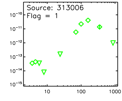
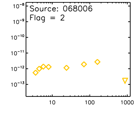
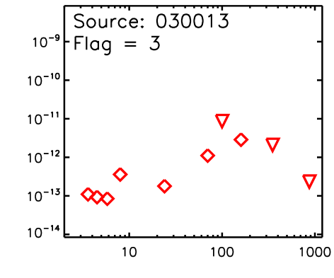
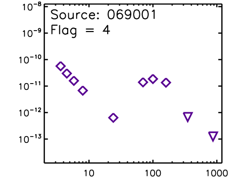
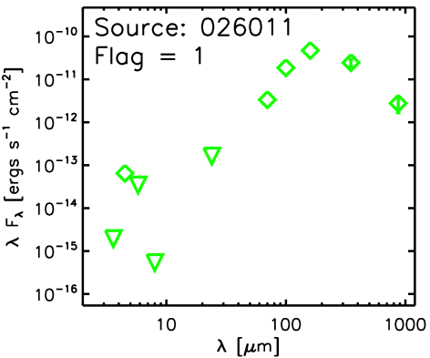
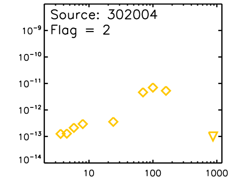
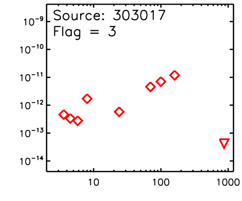
Figure 4.— Example SEDs for each of the 5 categories described in § 3.2: green SEDs (flag $=1$) are considered to be reliable protostar candidates, yellow SEDs (flag $=2$) are less likely to be protostellar, red SEDs (flag $=3$) are considered extragalactic contamination based on the 8 µm PAH feature, the purple SED (flag $=4$) is an example of one of 3 sources that may be explained as transition disks, and, finally, the black SED (flag $=5$) is unclassifiable due to the lack of IRAC coverage. Errors are smaller than the size of the points, except for the 350 µm and 870 µm points; upper limits are indicated with triangles.

3.1. Spitzer non–detections

A search for newly detected protostars using Herschel requires us to determine upper limits at 24 µm for those sources that are not detected by Spitzer. To determine these limits, we adapt the method developed by Megeath et al. to assess the spatially varying completeness of the Spitzer Orion Survey data. The completeness of the 24 µm data depends strongly on the presence of nebulosity and point source crowding. To account for these factors, we measure the fluctuations of the 24 µm signal in an annulus centered on the position of the Herschel point–source using the the root median square deviation, or RMEDSQ (see Equation 1 of Megeath et al., 2012). We then use the results from the artificial star tests (see Appendix of Megeath et al., 2012) to determine the magnitude at which 90% of the point sources would be detected for the observed level of fluctuations. We convert this magnitude into a flux density to obtain 24 µm upper limits.

Several of the identified protostars show IRAC emission but are not included in the Megeath et al. point source catalog because they are spatially extended. To obtain homogeneously extracted IRAC fluxes for the entire sample of sources, we measure fluxes using an aperture of 2 pixels, with a sky annulus of 2 to 6 pixels, corresponding to aperture radii of 2.44″, 2.44″, and 7.33″, respectively, with a pixel scale of 1.22″ pixel^-1. We use the PACS 70 µm source coordinates as starting guesses, and attempt to re–center at each IRAC wavelength. If the re-centering fails, as for sources with no IRAC detections, we take the integrated flux in that aperture at the original PACS 70 µm source coordinate to be the upper limit. The aperture corrections and photometric zero–points are those given by Kryukova et al.

3.2. Contamination in the sample

Galaxies often exhibit infrared colors similar to those of young stellar objects (YSOs) due to the presence of dust and hydrocarbons in the galaxies (Stern et al., 2005). Extensive work has been done towards characterizing the extragalactic “contamination” in Spitzer surveys of star–forming regions and mitigating it through photometric criteria designed to separate galaxies from bona fide YSOs (Gutermuth et al., 2009, 2008; Harvey et al., 2007). These authors show that star–forming galaxies can be distinguished from YSOs by the galaxies’ stellar–like emission in the IRAC 3.6 µm and 4.5 µm bands and their bright polycyclic aromatic hydrocarbon (PAH) emission in the IRAC 5.8 µm and 8.0 µm bands (Gutermuth et al., 2009, 2008; Winston et al., 2007; Stern et al., 2005). However, we note that some Active Galactic Nuclei (AGN) dominated galaxies may not exhibit PAH emission; therefore an analysis based only on the IRAC colors may not capture all possible sources of contamination (Robitaille et al., 2008).

To analyze the IRAC colors of our sample, we define $\alpha=dlog(\lambda F_{\lambda})/dlog(\lambda)$. In Figure 2, we plot $\alpha_{5.8-8}$ vs. $\alpha_{3.6-4.5}$ for the sample of new Herschel sources with coverage in all four of the Spitzer/IRAC bands and detections in at least one band, compared to the HOPS protostar sample. This color index is relatively insensitive to reddening since the extinction in the 5.8 µm and 8 $\mu$m bands of IRAC are very similar (e.g., Flaherty et al., 2007; Gutermuth et al., 2008). Figure 2 shows a cluster of sources with high values of $\alpha_{5.8-8}$ (i.e., $\alpha_{5.8-8}\geq 3$; solid horizontal line) yet $\alpha_{3.6-4.5}$ values of an SED that is declining or flat with increasing wavelength. These sources show the characteristics of star–forming galaxies with bright PAH emission (resulting in high values of $\alpha_{5.8-8}$) but values of $\alpha_{3.6-4.5}$ that are dominated by starlight. In our adopted scheme, $\alpha_{5.8-8}\geq 3$ corresponds to a color of $[5.8]-[8]\geq 2.17$; this threshold is higher than the $[5.8]-[8]\geq 1$ threshold used by Gutermuth et al. (2008) to isolate galaxies and thus ensures that most protostellar candidates will be less likely to be miss–identified extragalactic sources (Allen et al., 2004; Megeath et al., 2004). We identify the cluster of sources with $\alpha_{5.8-8}\geq 3$ and $\alpha_{3.6-4.5}\leq 0.5$ as likely extragalactic contamination. We note that nebular contamination of the photometry can cause PAH–like $\alpha_{5.8-8}$ values, and thus may cause us to over–estimate the extragalactic contamination. Of the 55 sources identified here as protostellar candidates we flag 23 as possible extragalactic contamination based on this criteria. However, other sources of contamination, such as AGN lacking PAH emission, may remain in our sample.

Inspection of the SEDs of the remaining 32 sources show a range of SED slopes and shapes. It is possible that such sources may also be extragalactic contamination by AGN, for example. To address this, we further refine the analysis presented above by analyzing the 3.6 µm to 160 µm SED shapes with the spectral index $\alpha_{3.6-160}$. As illustrated in Figure 3, the sources flagged as extragalactic based on the $\alpha_{5.8-8}$ index (red points) generally have $\alpha_{3.6-160}\lesssim 1.2$. We therefore calibrate the $\alpha_{3.6-160}$ relative the reliable extragalactic candidates with robust IRAC detections and expect that extragalactic sources will have $\alpha_{3.6-160}\lesssim 1.2$. Using this criterion, we refine our source classification as follows. All sources with $\alpha_{3.6-160}>1.2$ (and $\alpha_{5.8-8}<3$ when IRAC detections exist) are flagged as high probability protostars (flag $=1$ in Table 3). Sources having values of $0.5\lesssim\alpha_{3.6-160}\lesssim 1.2$ but that originally classified as candidate protostars based on a low value of $\alpha_{5.8-8}$ are flagged as less likely to be of a protostellar nature (flag $=2$ in Table 3). Furthermore, by definition, sources originally classified as extragalactic based on their PAH signature at 8 µm remain classified as such (flag $=3$ in Table 3). Sources with $\alpha_{3.6-160}<0.3$ and $\alpha_{3.6-4.5}\sim-3$ are flagged as “other” (flag = 4 in Table 3) since their SEDs are consistent with a stellar photosphere at shorter wavelengths. Finally, one source has no IRAC coverage and therefore is flagged with a value of 5. In Figure 4 we show example SEDs of each category.

Only one source (313006) originally flagged as extragalactic based on its $\alpha_{5.8-8}$ limit (non–detection at 5.8 µm and 8 µm) was revised to a highly probable protostar (see Figure 3 and top left panel of Figure 4). In addition, as we note above, we find three sources with SEDs that we label “other” (flag value $=4$) which are inconsistent with the categories described above. Source 069001 (see Figure 4, top right panel) was previously characterized by Fang et al. (2009) as a K7 star with a debris disk, with a very poorly constrained age of $\sim 0.06^{+4.66}_{-0.03}$ Myr. These authors only include data up to 24 µm. The SED we observe with Herschel may be consistent with a transition disk but not a debris disk. The remaining two sources in this category have similar SEDs as that of 069001; while a transition disk explanation for all three sources may appear likely depending on the age of the sources, we cannot currently rule out other possibilities. Nevertheless, all of these sources have SEDs consistent with a stellar photosphere in the IRAC bands, and hence these are likely to be fully formed stars surrounded by circumstellar dust.

Interestingly, we find that the most reliable SED classification criterion by far is that of sources that have neither IRAC nor MIPS 24 µm detections. Of these, we find that all 6 sources have strong sub–millimeter detections and reside in dense and filamentary environments. This finding points to the critical importance of obtaining high resolution sub–millimeter data to constrain the properties of such sources. In the following text, we include all 55 Herschel–detected sources in our analysis and figures.

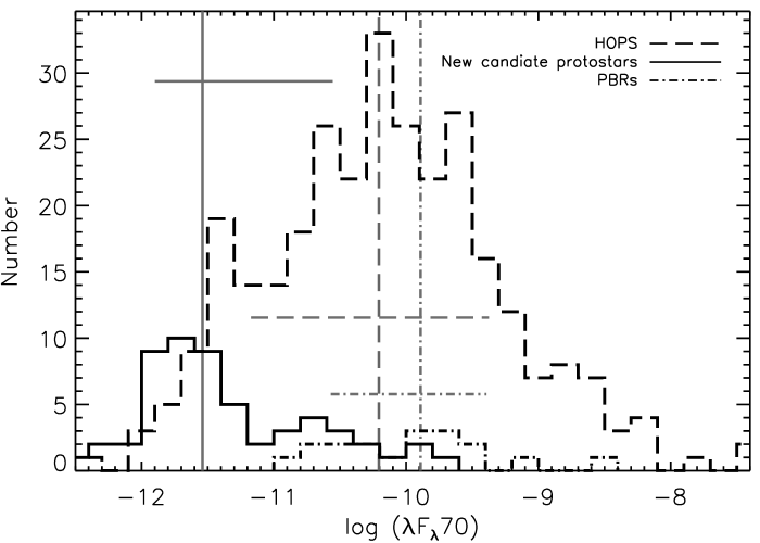
Figure 5.— Distributions of 70 µm fluxes for the HOPS protostars (dashed histogram), new candidate protostars (solid histogram), and the 18 reddest sources drawn from both combined samples (dot–dashed histogram). The corresponding grey lines indicate the median flux values (vertical lines) and the 68% interval (horizontal lines).

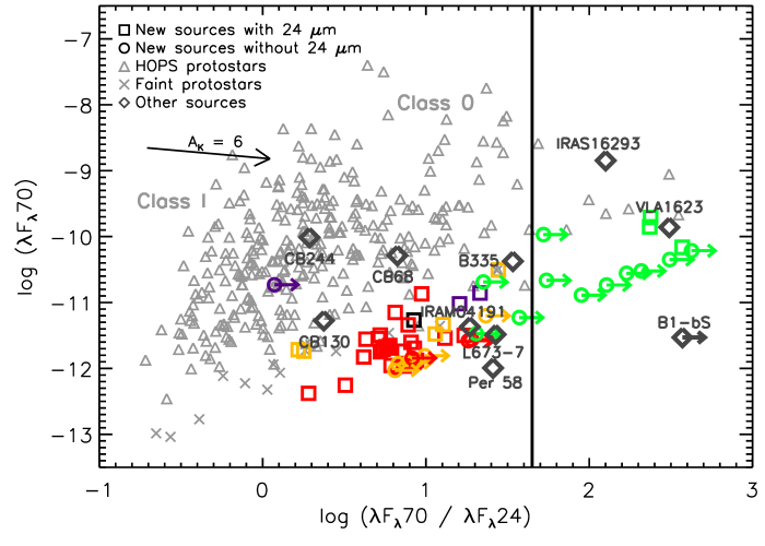
Figure 6.— Top: 70 µm flux vs. 70 µm to 24 µm flux ratio for HOPS–detected Orion protostars. Open squares and open circles indicate the new candidate protostars with and without MIPS 24 µm detections, respectively. The color of the symbols indicates the flag values shown in Table 3 and discussed in § 3.2: here, green indicates sources that are reliable protostar candidates (flag $=1$), orange indicates less reliable sources (flag $=2$), red indicates extragalactic contamination (flag $=3$), purple indicates other sources (flag $=4$), and black indicates the single source without IRAC coverage. The solid vertical line indicates a 70 µm to 24 µm flux ratio of 1.65, our PBRs selection criterion (see § 5). Triangles and $\times$ symbols indicate previously detected and characterized Spitzer protostars and faint protostellar candidates from Megeath et al. (2012), respectively. The arrow indicates the extinction vector for a value of $A_{K}=6$. For comparison, we also indicate as large diamonds the scaled observed measurements for some well–known Class 0 sources, VeLLOs, and two FHSC candidates (see text). Bottom: 160 µm to 70 µm flux ratio vs. 70 µm to 24 µm flux ratio for HOPS–detected Orion protostars. The symbol and color type is the same as in the top panel. The reddest sources are distinguished from the bulk of Spitzer–identified HOPS sources (triangles) both by brighter 160µm fluxes and redder 70 µm to 24 µm flux ratios.

4. Herschel protostar candidates

We present the Herschel protostar candidate catalog in Table 3. Here we include the PACS 70 µm coordinates and flux measurements at 24 µm, 70 µm, and 160 µm. We indicate which sources are flagged as reliable protostellar candidates and which are likely contamination, based on the results from the previous section. We also indicate if the sources have a robust 870 µm detection. Furthermore, we present the values of L_bol and T_bol and their corresponding estimated statistical errors (see discussion in § 5.1). In Figure 5, we show the 70 µm flux distributions for the sample compared to the distribution of HOPS protostars. The majority of the new candidate protostars have 70 µm fluxes that are lower than the previously identified Spitzer HOPS sample; this is not surprising since the new candidate protostar sample is selected to be faint or undetected at 24 µm. Furthermore, the peak at low 70 µm flux values is dominated by extragalactic contamination, as discussed above.

In Figure 6, we show the MIPS 24 µm, PACS 70 µm, and PACS 160 µm colors of the new Herschel sources compared to the HOPS sample of 70 µm detected protostars. The top panel shows the 70 µm flux vs. the log $(\lambda F_{\lambda}70/\lambda F_{\lambda}24)$ color (henceforth $70/24$ color), while the bottom panel shows the log $(\lambda F_{\lambda}160/\lambda F_{\lambda}70)$ color (henceforth $160/70$ color) vs. the $70/24$ color, for our sample of new protostar candidates compared to the colors of the Spitzer–identified HOPS sample. The Spitzer 24 µm 7 magnitude limit, imposed on the HOPS sample for a reliable protostellar identification, is apparent in the top panel as the diagonal line approximately separating the new protostellar candidates at fainter 70 µm fluxes and redder $70/24$ colors from the population of Spitzer–identified HOPS sources.

For comparison, in the top panel of Figure 6, we also show the fluxes and colors of presumably typical and well–studied Class 0 sources: VLA1632–243 (J. Green and DIGIT team, private communication, 2012, and Green et al., in prep.), IRAS16293 (Evans et al., 2009), B335 (Stutz et al., 2008; Launhardt et al., 2012), CB68 (Launhardt et al., 2012), and CB244 (Stutz et al., 2010; Launhardt et al., 2012). Furthermore, we also show the colors of various VeLLOs: L673–7 (Dunham et al., 2008), IRAM04191 (Dunham et al., 2006), and CB130 (Launhardt et al., 2012). We find that the observed colors of our sample of candidate protostars appear consistent with the colors of more near–by Class 0 and VeLLO sources but not with FHSC candidate colors proposed in the literature (e.g., Commerçon et al., 2012). We find that the majority of these previously known Class 0 and VeLLO sources do not appear as red in their $70/24$ colors as the reddest sources in our sample. The only exceptions to this trend are IRAS16293 and VLA1632–243, perhaps representing an extrema in the $70/24$ color distribution that may be driven by their comparatively large envelope densities.

We also show in Figure 6 the colors of two FHSC candidates in Perseus: Per–Bolo 58 (Enoch et al., 2010) and B1-bS (Pezzuto et al., 2012). In this diagram, the $70/24$ color of Per–Bolo 58 appears generally consistent with that of a VeLLO, as Enoch et al. (2010) point out. As such, this source may be an extremely low–mass protostar. On the other hand, the $70/24$ color of B1-bS is comparable to the very reddest sources we find in Orion while the 70 µm flux is consistent with VeLLOs and fainter than the reddest sources in Orion by more than one order of magnitude. The faint but robust detection of a 70 µm point–source by Pezzuto et al. (2012) may indeed point to the possible Class 0 or VeLLO nature of B1-bS. We do however note that Pezzuto et al. also detect a source with no 70 µm counterpart, B1–bN, which may therefore represent a more robust FHSC candidate. Regardless of the elusive nature of FHSC candidates, when comparing our new candidate protostar colors to FHSC models by Commerçon et al. (2012), we find that our sources do not appear to be consistent with predicted or expected FHSC colors, with the caveat that distinguishing FHSCs from VeLLOs with continuum observations alone is likely difficult.

5. PACS Bright Red Sources

Up to this point, we have discussed two distinct and well–defined samples of sources in Orion: i) the sample of candidate protostars identified with Herschel that have PACS 70 µm and 160 µm detections but MIPS 24 µm magnitudes greater than 7.0 mag, ii) the sample of protostars that were reliably identified with Spitzer (24 µm magnitudes $\leq 7.0$ mag Megeath et al., 2012; Kryukova et al., 2012). The protostar catalog target list used for the HOPS program consists mostly of the Spitzer identified protostars, but also contains some of the previously known protostars with $m(24)>7.0$ mag (Fischer et al., in preparation).

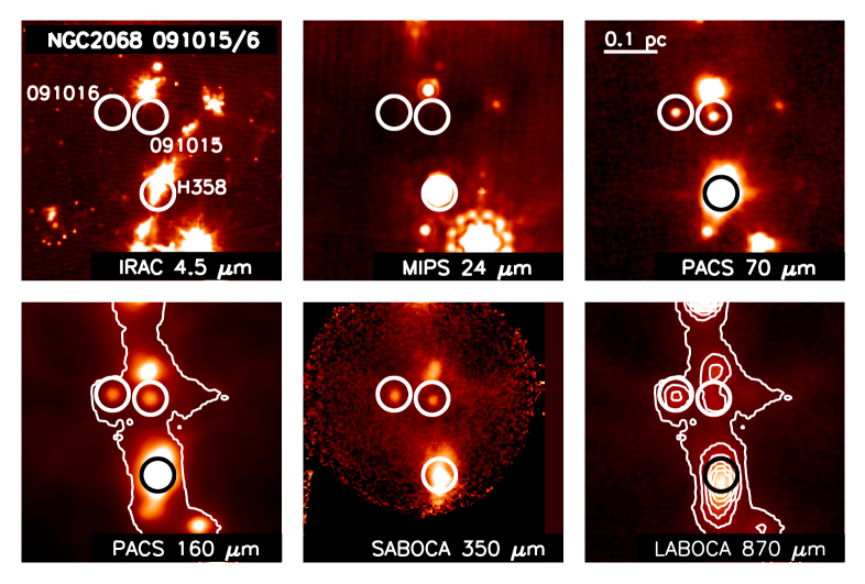
Figure 7.— $4\arcmin\times 4\arcmin$ images of three PBR sources, 091015 and 091016 (top), and HOPS358 (bottom), at the indicated wavelengths, shown on a log scale. North is up, east is to the left. The circles indicate the location of the PACS 70 µm point–sources. Contours indicate the 870 µm emission levels at {0.25, 0.5, 0.75, 1.0, 1.25} Jy beam^-1. The lowest 870 µm contour is over–plotted on the 160 µm image. No IRAC emission coincident with 091015 or 091016 is detected; however, these sources clearly reside in dense filamentary material traced by the sub-mm emission. The HOPS358 photometry is likely blended.

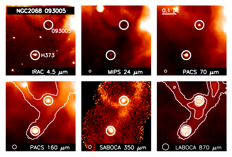
Figure 8.— Same as Figure 7, showing $4\arcmin\times 4\arcmin$ images two PBRs: 093005 (top) and HOPS373 (bottom). Contours indicate the 870 µm emission levels at {0.25, 0.5, 0.75, 1.0, 1.25, 1.5} Jy beam^-1. Source 093005 is the reddest PBRs shown in Figure 6 and lies at the intersection of three filaments traced by an 8 and 24 µm absorption feature and the 870 µm emission.

In what follows, we focus our analysis on the Orion protostars that have $70/24>1.65$. Of the 18 known protostars that satisfy this limit, 11 are identified with Herschel; hence this color regime is dominated by our newly identified protostars. Accordingly, Herschel has provided us for the first time with a far more complete sample of these red sources within the field of the HOPS survey. Given their red colors and their brightness in the PACS wavelength bands, we refer to this sample of protostars as PACS Bright Red sources, or PBRs. The coordinates, Spitzer photometry , and Herschel photometry of the sample are listed in Table 4, while the APEX 350 µm and 870 µm photometry are presented in Table 5. Since the APEX photometry are non–trivial to extract due in large part to contamination by cold surrounding material and, at 870 µm specifically, by the large beam size, we present three measures of the source flux, as described above.

5.1. Observed properties PBRs

As discussed above, we select 18 PBRs in Orion with observed $70/24$ colors greater than $1.65$. We show 4.5 µm to 870 µm images of 5 example PBRs in Figures 7 to 8 (see Appendix for the full sample images). Furthermore, in Figure 9 we show the full set of 18 PBRs observed SEDs from 24 µm to 870 µm. Inspection of the observed SEDs confirms that the PBRs sample is composed of cold, envelope dominated sources with peak emission always located at $\lambda>70$ µm. In addition, the peak of the SEDs, and thus the temperatures, are well–constrained for all PBRs because we have obtained APEX sub–millimeter coverage for all sources.

In Table 6, we present some basic properties of the PBRs. In particular, we find that 12/18 sources exhibit Spitzer 4.5 µm emission indicative of outflow activity. We also include some references to previous detections (see Appendix). Furthermore, 4/18 sources have significant levels of 4.5 µm emission that are indeed consistent with a high inclination. The majority of sources, however, do not give clear indications of their inclinations at any observed wavelength, and therefore we cannot make any statements about their possible orientations based on their appearance in the images. We find indications from the 4.5 µm image morphology that two sources (HOPS341 and HOPS354) are binaries, while seven sources have a nearby source within $30\arcsec$. Two reside in more crowded regions, and seven sources appear truly isolated. We find that a significant fraction (13/18) of sources appear to reside in filamentary regions, i.e., the extended 870 µm emission appears significantly elongated.

The four sources with significant indications of a high inclination orientation are HOPS169, 302002, HOPS341, and HOPS354 (see Appendix for Figures 17, 21, 23, and 25). Inspection of their 4.5 µm images reveals that their outflows appear well collimated and relatively narrow. Indeed, we might expect that sources that that have denser envelopes, and are therefore presumably younger, may have more narrow cavity opening angles (e.g., Arce & Sargent, 2006). As an additional check on our density analysis (see above), we use this inclination information for an independent check of the envelope densities of these four sources. Despite the relatively sparsely sampled SEDs, we fix the inclination to $87^{\rm o}$ and fit the source SEDs. We find that even when we fix the model inclination to $\theta=87\mbox{${}^{\circ}$}$, we still obtain envelope densities significantly above the $\rho_{1}$ value found in the previous section.

Figure 9.— SEDs of the 18 PBRs are shown. The errors are smaller than the symbol size except for the 350 and 870 µm data points. The black curve shows the modified black–body fit to the observed SED, with the indicated best fit parameters (see § 6.2). Note that PBRs 19003 (shown in the top right) is located in a complex field where the photometry may be strongly contaminated.

5.2. Observational evolutionary diagnostics

We calculate L_bol, T_bol (Myers & Ladd, 1993), and L_smm/L_bol (André et al., 1993, 2000). The errors in L_bol and T_bol are derived with the same Monte Carlo method as described in § 6.2 for the modified black–body parameters. We exclude the IRAC upper limits from this analysis; including these limits has an effect on our L_bol and T_bol estimates that is smaller than our estimated errors. We do, however, include the 24 µm upper limits; therefore the L_bol and T_bol values should be considered upper limits for sources not detected at this wavelength. Furthermore, we investigate the effect of applying an average foreground reddening correction to all the new Herschel candidate protostars. We find that dereddening the observed fluxes with extinction levels of $A_{V}=40$ magnitudes has no effect on the derived parameters because the observed SEDs are extremely red and cold.

5.3. Spatial distribution of the three samples

We show the locations of the Herschel protostar candidates compared to the locations of the HOPS sample in Figure 10; these positions are overlaid on the extinction map of Orion. It is immediately apparent that the spatial distribution of the new candidate protostars and PBRs is non–uniform. To investigate this distribution further, we show the relative fraction of new sources as a function of individual region in Table 7. The over–all number of new candidate protostars and PBRs is dominated by the Orion A cloud, and in particular L1641. This is not surprising since the L1641 region is quite large and contains more protostars compared to other Orion regions. The fractions of new candidate protostars and PBRs compared to the total number of HOPS and new candidate protostars is, however, 2 times larger in Orion B. This result is even more pronounced when we consider only the fractions of PBRs, with fractions that are more than 10 times larger in Orion B. The NGC2068 (also containing the NGC2071 nebula) and NGC2024 (also containing the Horsehead or NGC2023 nebula) fields in Orion B have not only the largest fraction of new candidate protostars, but also of PBRs. While these numbers and fractions are subject to counting statistics and other possibly large sources of errors, the differences between Orion A and Orion B appear to be significant.

About 5% of the combined protostars and candidate protostars in Orion are PBRs. If we consider the PBRs as representing a distinct phase in the evolution of a protostar, and we assume a constant rate of star formation, the fraction the variation suggests that the protostars spend 5% of their lifetime in the PBRs phase (approximately 25,000 years with the 0.5 Myr protostellar lifetime of Evans et al., 2009), averaging over all Orion regions. However, the assumed the duration of the PBRs phase would vary greatly with location, from $5,000$ years in the Orion A cloud to $80,000$ years in the Orion B cloud. There are two alternative explanations. First, there might be environmental reasons which would favor the formations of PBRs, or perhaps extend the duration of the PBRs phase, in the Orion B cloud. Second, the ages of all the protostars in the Orion B cloud may be systematically younger than those in the Orion A cloud. In this case, the regions containing the PBRs in the Orion B could be undergoing very recent bursts of star formation.

Studies of pre–main sequence stars in the Orion molecular clouds show little evidence for significant age differences between the Orion A and B clouds. Flaherty & Muzerolle (2008) determined an age of $\sim\,$2 Myr for NGC2068 and NGC2071, while Reggiani et al. (2011), Hsu et al. (2012) and Da Rio et al. (2012) determine ages for the ONC and L1641 of $\sim\,$2 — 3 Myr. However, most of the protostars associated the NGC2068 and NGC2071 regions are outside the clusters of pre–main sequence stars and in dense filaments gas neighboring these clusters (Motte et al., 2001). A number of PBRs are in the LBS 23 clump (directly south of NGC2068) and in the NGC2023 clump (in the NGC2024 field); these are two of the 5 most massive, dense clumps found in Orion (Lada et al., 1991a). Compared to the other massive clumps, both of these regions have $1/10$ the numbers of young stars per unit gas mass and hence may be quite young (Lada et al., 1991b; Lada, 1992). Alternatively, the gas in the LBS 23 and NGC2023 clumps may have dense gas filling factors that are much higher than the other massive clumps (Lada et al., 1997); hence, they sources in these regions may be forming in a very different birth environment. The regions bordering the southern rim of the NGC2068 nebula and the northern rim of the NGC2071 nebula are also rich in protostars (see Megeath et al., 2012). Thus, the PBRs are found concentrated in sub–regions which may indeed be quite young. We will investigate these possibilities in future work.

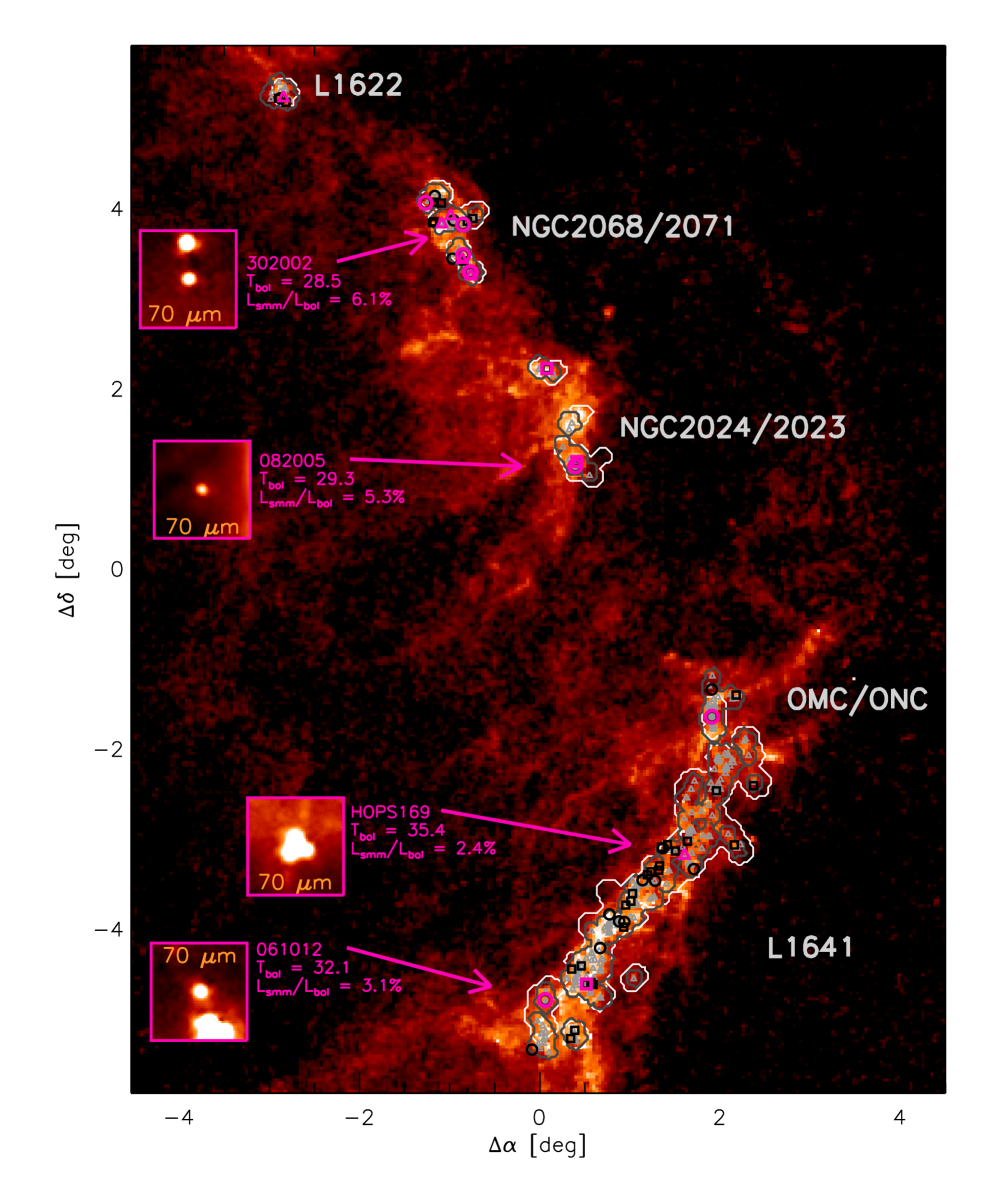
Figure 10.— The distribution of red protostars overlaid on the extinction map of Orion. The dark grey contour shows the HOPS PACS coverage and the white contour shows the LABOCA 870 µm coverage. The triangles (light grey) indicate the positions of the HOPS protostars while the black points (squares and circles) indicate the positions of the new candidate protostars. The PBRs are highlighted in fuchsia and the properties of four selected PBRs are shown along with their corresponding $1\arcmin\times 1\arcmin$ HOPS 70 µm images.

6. Determining the Physical Properties of PBRs through models

In this section we describe our analysis of the physical properties of the PBRs as inferred from their colors and SEDs. We first compare the $70/24$ colors of the PBRs sample with those derived from a grid of models which adopt the solution for a rotating envelope undergoing collapse (Ulrich, 1976; Terebey et al., 1984) with outflow cavities along the rotation axis of the envelope (Whitney et al., 2003a). This analysis puts a constraint on the minimum inner density of the protostellar envelope. Next, we compare the observed SEDs to model SEDs generated using the Hyperion (Robitaille, 2011) radiative transfer code. This set of models assumes radial power–law gradients consistent with either a collapsing core with a constant infall rate and a static isothermal core. The models also encompass various combinations of internal and external heating. Given the prohibitively large computational time needed to explore the full range of parameters space using radiative transfer models, and given our inability to distinguish between models purely from five to six photometry points, we do not provide individual model fits to each protostars. Instead we fit a single temperature modified black–body function to the observed SEDs at 70 µm and longer wavelengths. The modified black–body fits provide luminosities and an initial characterization of the envelope masses of the PBRs sample.

6.1. Axisymmetric models: interpreting the $70/24$ color

We begin our analysis by using a simplified version of the Ali et al. (2010) protostellar envelope model grid to predict observed fluxes and colors for comparison with our PBRs. The density distribution of these models is that of the collapse of a spherical cloud in uniform rotation (Ulrich, 1976), which is the inner region of the Terebey et al. (1984) model of the collapse of the slowly–rotating isothermal sphere. This model is then modified by the inclusion of outflow cavities of various shapes (Whitney et al., 2003a, b). This schematic model envelope captures the dependence of the short wavelength (24 µm and 70 µm) fluxes on inclination due to rotation and bipolar cavities.

The model fluxes depend upon the mass infall rate, the angular momentum of the mass currently falling in, the outflow cavity properties, the inclination of the rotation axis to the line of sight, and the luminosity of the central source, as well as the assumed dust properties. The thermal emission of the dusty envelope does not depend directly on the mass infall rate but instead on the density of the envelope. The model assumes free–fall at a constant rate, which results in a density profile with shape $\rho\propto r^{-3/2}$ (Terebey et al., 1984) . The overall scaling of the density is characterized by $\rho_{1}$, the density at 1 AU in the limit of no rotation:

$$\rho_{1}=7.4\times 10^{-15}\Bigg{(}\frac{\dot{M}_{\rm env}}{10^{-6}{M}_{\odot}\,{\rm yr}^{-1}}\Bigg{)}\Bigg{(}\frac{M_{*}}{0.5\,{M}_{\odot}}\Bigg{)}^{-1/2}\rm{g\,cm}^{-3},$$ (1)

The envelope mass infall $\dot{M}_{\rm env}$ rate is related to $\rho_{1}$ via the free–fall velocity, which in turn depends upon the unknown central mass ${M}_{*}$. The actual model density structure departs from $r^{-3/2}$ on small scales because of the angular momentum of the infalling material. This enters into the model through the parameter $R_{\rm disk}$, the outer disk radius at which infalling material currently lands (see Ulrich, 1976).

The rotation leads to a significant dependence of the SED on the inclination of the rotation axis relative to the line of sight (Kenyon et al., 1993). This dependence is significantly enhanced by the inclusion of outflow cavities (Whitney et al., 2003a) which are assumed to be aligned along the rotation axis. Finally, the overall shape of the SED is only weakly affected by the luminosity of the central source ($L_{*}$; Kenyon et al., 1993) and so this is easily scaled.

To roughly compare observed PBRs colors with those predicted by our model grid in Figure 11 we show the effects of varying the model inclination, envelope density, and cavity opening angle on the $70/24$ color and 70 µm flux. As stated above, these model tracks are based on a simplified version of the Ali et al. (2010) model grid; we refer the reader to that publication for details. In brief, the model tracks that we consider here have the same fixed parameters as those listed in Table 1 of Ali et al. (2010), including a fixed central mass of $0.5$ $\hbox{M}_{\odot}$; in addition we have fixed the cavity shape exponent to a value of $b=1.5$, and the envelope outer radius to $R_{\rm env,max}=1\times 10^{4}$ AU. We have, however, expanded the envelope infall rate grid relative to the Ali et al. (2010) grid to larger values (up to $\dot{M}_{\rm env}=10^{-3}$ $\hbox{M}_{\odot}$ yr^-1 on a pseudo–logarithmic grid) and included a model with no envelope. As described above, for our model grid we assume that the envelope density falls off as $\rho(r)\propto r^{-3/2}$. In addition, while our model grid is parametrized in terms of $\dot{M}_{\rm env}$, with a fixed central mass of $M_{*}=0.5$ $\hbox{M}_{\odot}$, we will refer to $\rho_{1}$ throughout this section.

We note that the assumed central masses of protostellar sources remain largely unconstrained observationally (however see Tobin et al., 2012), but may be lower than our assumed value. The effect of a lower central mass would be to lower $\dot{M}_{\rm env}$ for a given value of $\rho_{1}$. For example, if the central mass is $0.2$ $\hbox{M}_{\odot}$, the infall rates reported for our models would be reduced by a factor of 0.6. The assumed central mass, however, does not change the value of $\rho_{1}$ corresponding to a given model SED. Furthermore, our small assumed disk radius does not strongly affect the trends shown here.

With this model grid we isolate the effects, albeit in a simplified fashion, of varying the model inclination (viewing angle to the protostar), envelope density ($\rho_{1}$), and cavity opening angle ($\theta_{\rm C}$) on the 70 µm fluxes and $70/24$ colors. In Figure 11, we show model tracks through 70 µm flux vs. $70/24$ color space for high inclination ($87^{\rm o}$) viewing angles as a function of both $\theta_{\rm C}$ and envelope density ($\rho_{1}$). By analyzing only the high inclination models we obtain a lower limit on the envelope density required to reproduce the red $70/24$ colors.

We assume a fixed disk accretion rate of $\dot{M}_{\rm disk}$ $=1.0\times 10^{-8}$ $\hbox{M}_{\odot}$ yr^-1, a disk outer radius of $R_{disk,max}=5$ AU, and a central source luminosity of $1$ L_⊙. Increasing $\dot{M}_{\rm disk}$ and $R_{disk,max}$ drives the models to both bluer $70/24$ colors and brighter 70 µm fluxes, while decreasing the inclination drives the models to bluer $70/24$ colors. Therefore, we find that no model in our grid can explain $70/24$ colors with envelope densities less than log $\rho_{1}/({\rm g\,cm}^{-3})\sim-13.4$ (or equivalently an envelope infall rate of $\dot{M}_{\rm env}$ $=5.4\times 10^{-6}$ $\hbox{M}_{\odot}$ yr^-1). While models with larger values of $\rho_{1}$ and other combinations of parameters can be found for bluer $70/24$ colors, this analysis sets an approximate lower limit on the expected envelope densities of sources with $70/24>1.65$ of log $\rho_{1}/({\rm g\,cm}^{-3})\gtrsim-13.4$. That is, high source inclinations alone cannot explain the red $70/24$ colors of the PBRs, which also require dense envelopes.

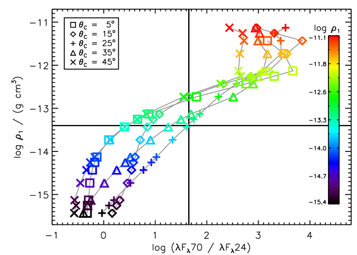
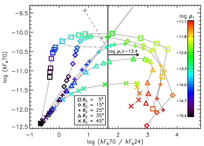
Figure 11.— Left: Dependence of the model 70 µm to 24 µm flux ratio for high inclination orientations ($87^{\rm o}$) on envelope density ($\rho_{1}$) for the 5 cavity opening angels in our grid. These model tracks assume an internal luminosity of 1.05 L_⊙. The $70/24$ color selection is indicated with the vertical black line, while the corresponding log $\rho_{1}/(g\,cm^{-3})\sim-13.4$ (corresponding to an envelope infall rate of $\dot{M}_{\rm env}$ $=7.5\times 10^{-6}$) threshold is indicated with a horizontal black line. Right: Model 70 µm flux vs. 70 µm to 24 µm flux ratio for high inclination orientations ($87^{\rm o}$). For the model with a cavity opening angle of $\theta_{\rm C}=25^{o}$ ($+$–symbols) and log $\rho_{1}/(g\,cm^{-3})\sim-13.4$, we show the effect of of increasing the internal luminosity by two orders of magnitude with the dashed grey curve while the effect of decreasing the inclination to $18^{o}$ is illustrated with the dot–dashed curve. All models with higher assumed values of $\dot{M}_{\rm disk}$ and lower inclination will have envelopes that are denser than log $\rho_{1}/(g\,cm^{-3})\sim 13.3$, the median value of $\rho_{1}$ in our model grid; sources with redder 70 to 24 µm colors cannot be explained by envelopes that are less dense than this threshold. The light grey thick line corresponds to a 24 µm limit of 7 magnitudes, the imposed Spitzer protostar magnitude limit for identification of protostars.

We expect that this value of $\rho_{1}$ should lie well within the Class 0 range; e.g., Furlan et al. (2008) found for a sample of 22 Class I sources in Taurus log $\rho_{1}/({\rm g\,cm}^{-3})\leq-13.2$, while over half had $\rho_{1}$ values that are lower than log $\rho_{1}/({\rm g\,cm}^{-3})=-13.4$. Note that the Furlan et al. (2008) data–set included far better sampling of the source SEDs and, most critically, Spitzer IRS spectroscopy, allowing for a more robust estimate of the parameters of sources in their sample. In contrast, our SEDs generally are envelope dominated with few sources having robust detections shortward of 24 µm. Therefore, any estimate of the value of the envelope density will be necessarily imprecise and have a back of the envelope character. That said, our comparison with the model grid and previous derived values of the envelope density leads us to conclude that the $70/24>1.65$ color cut, while not uniformly selecting a unique envelope density threshold, will preferentially select Class 0 sources with log $\rho_{1}/({\rm g\,cm}^{-3})\gtrsim-13.4$, irrespective of source inclination.

Having demonstrated that the very red $70/24$ colors require large values of $\rho_{1}$, as expected for SEDs peaking at long wavelengths, we proceed by analyzing the PBRs in the context of more simplified models. In what follows, we carry out two independent analyses of the source SEDs: a qualitative model image comparison using 1D models generated with the Hyperion (Robitaille, 2011) radiative transfer code, and modified black–body fitting to the observed SEDs at 70 µm and longer wavelengths. We attempt to maintain consistency by using similar envelope dust models throughout the analysis presented here. For the Hyperion model image analysis we use the Ormel et al. (2011) opacities. These opacities are similar to the commonly assumed Ossenkopf & Henning (1994) (“OH5”; see below) opacities but include both the scattering and absorption components at short wavelengths, needed for radiative transfer calculations. Specifically, we use the “icsgra2” Ormel et al. (2011) model opacities, which include icy silicates and bare graphites, with a coagulation time of 0.1 Myr. We assume the dust model from Ossenkopf & Henning (1994) for the long–wavelength modified black–body fits, specifically, their “OH5” opacities, corresponding to column 5 of their Table 1. These opacities reflect grains having thin ice mantles with $10^{5}$ years of coagulation time at an assumed gas density of $10^{6}$ cm^-3.

6.2. Spherically symmetric models: Comparison to photometry derived from model images

We use the Hyperion (Robitaille, 2011) Monte Carlo radiative transfer code to investigate some basic properties of the PBRs. We run a series of spherically symmetric models under a range of very simple assumptions, and produce simulated images. As stated above, the dust model we assume is that of Ormel et al. (2011) (”icsgra2”). To explore which model assumptions might be reasonable for analyzing the properties of the reddest sources in Orion, we investigate a few limiting model scenarios. We therefore disregard the details of the individual source SEDs of the entire red sample and qualitatively compare the SEDs of the two sources with the smallest and largest values of L_bol and T_bol (sources 091016 and HOPS358, respectively; see Table 8) with photometry derived from model images.

We generate a series of model images that fall into four classes: i) a starless core at a constant temperature of 10 K (referred to here as the “core” model); ii) a starless core with an isotropic external radiation field (“core$+$external”); iii) a core with an internal source (“star” model); and finally, iv), a core with both an internal source and an isotropic external radiation field (“star$+$external”). For each of these classes of models, we test a range of density profile shapes and density normalizations. For the density profile shape we assume two values, $\alpha=1.5,2.0$, where $\alpha$ is the radial density profile power law index: $\rho(r)\propto r^{-\alpha}$. For the absolute value of the (gas) density normalization at 1 AU we assume 5 values: $\log{(\rho_{1{\rm AU}}/(g\,cm^{-3})})=-10$ to $-14$, in steps of $\delta\log{(\rho_{1{\rm AU}}/(g\,cm^{-3})})=1.0$. For models with external heating, the bolometric strength of the interstellar radiation field (ISRF) is set to the value from Mathis et al. (1983) at the solar neighborhood ($4\pi\,J_{\nu}=0.0217$ ergs/cm²/s). The spectrum of the radiation field is assumed to be that at the solar neighborhood from Porter & Strong (2005), but reddened by $A_{\rm V}=10$ using the Kim et al. (1994) extinction law. The ISRF model includes contributions from the stellar, PAH, and FIR thermal emission. The inner radius of the core is set to the radius at which the dust sublimates, assuming a sublimation temperature of 1,600 K, while the outer radius is set to 1 pc. The central source is taken to have 10 L_⊙ and a spectrum given by a Planck function at the effective temperature of the Sun (5778 K). The choice of the stellar temperature is arbitrary, and is unimportant for the modeling presented here, since all sources are deeply embedded and all stellar radiation is reprocessed — only the total bolometric luminosity is important (see e.g., Johnston et al., 2012, for a discussion of the R_star and T_star degeneracy).

The high levels of spatial filtering caused by our adopted aperture photometry scheme require us to assume such a central source luminosity to roughly match the flux levels in the observed SEDs. Furthermore, while a 1 pc sized envelope is larger than usually assumed, the high levels of spatial filtering inherent in the aperture photometry cause us to be insensitive to structure on scales larger than the assumed aperture sizes.

The model images have a resolution of 1$\arcsec pix^{-1}$, or 420 AU at our assumed distance. We convolve these images with the azimuthally averaged PSFs provided by Aniano et al. (2011), except in the case of the SABOCA 350 µm and LABOCA 870 µm images. These wavelengths are convolved with Gaussian PSFs with FWHMs equal to 7.4$\arcsec$ and 19$\arcsec$ respectively, i.e., the nominal beam sizes for our observations. All model image photometry is then performed on the convolved model images using the same aperture and sky annulus parameters as those applied to the data. The use of such photometric aperture parameters can cause large amounts of spatial filtering due the small sizes of the apertures relative to the beam sizes and the extent of the core emission (see below).

We show our extracted model SEDs in Figure 12 and a subset of the corresponding model images in Figure 13. In general, we find that models without internal sources are very unlikely to match the observed PBRs properties, on the basis that their SEDs are less luminous and peak at longer wavelengths than the observed SEDs for all density profile shapes that we assume; see Figure 12, top panels. While the ”core+external” models (top right panel) suffer from severe spatial filtering, it is unlikely that such models will well represent the data as these SEDs tend to also peak at longer wavelengths. For the two classes of models with internal sources we find better agreement with the data; see lower panels of Figure 12. While steeper envelope profiles may imply somewhat higher envelope densities, the range in plausible densities for $\alpha=1.5$ is $\log\rho_{1}\,\sim\,-12$ to $-13$, while for $\alpha=2.0$ values of $log\rho_{1}\,\sim\,-12$ roughly agree with the shapes the observed SEDs. We note that we find very little difference between the “star+external”and the ”star” model in the $\lambda\lesssim 160$ µm regime, possibly indicating that our assumed ISRF strength relative to the assumed internal source luminosity may be underestimated compared to what we might expect to find regions like Orion.

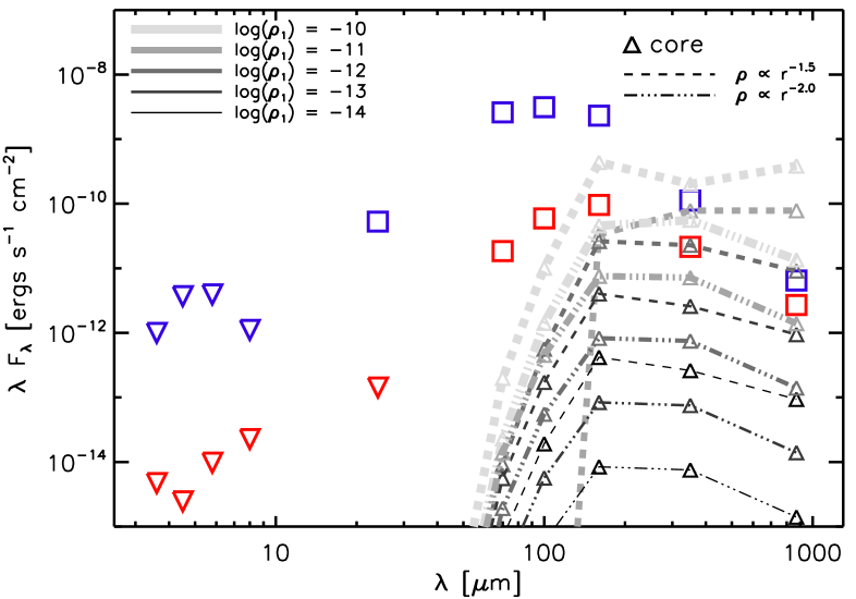
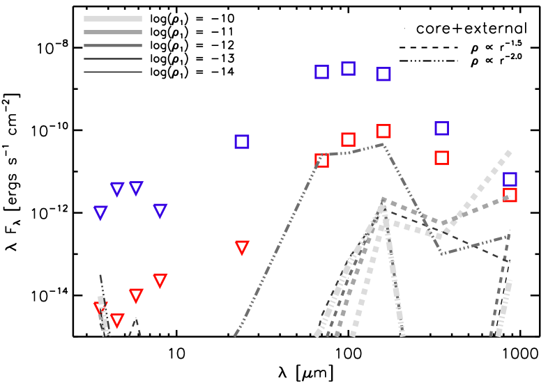
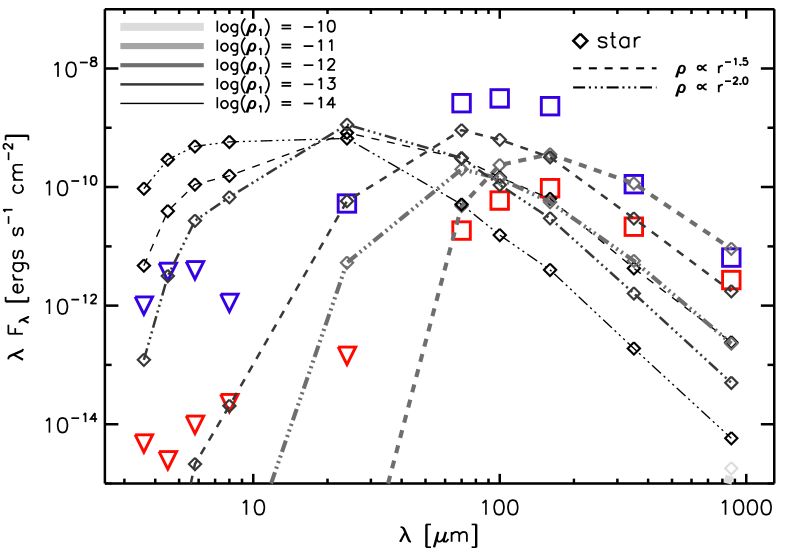
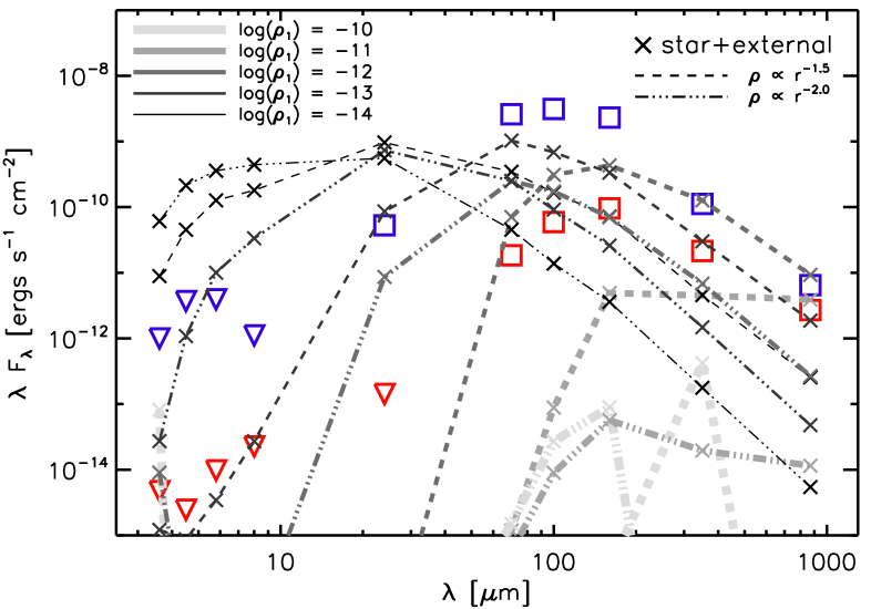
Figure 12.— All panels show the SEDs of HOPS358 (blue; L_bol = 30.6 L_⊙ and T_bol = 44.2 K) and 091016 (red; L_bol = 0.65 and T_bol = 29 K), the extrema of the L_bol and T_bol distributions for the reddest sources, compared to spherical models. The two line styles indicate the different assumptions for the density profile shape while the shade of grey indicates the different model density $\rho_{1}$ values. The four panels correspond to the four different models that we test (see text): Top left: the “core” model, a starless core; Top right: the “core+external” model, a starless core with external heating; Bottom left: the ”star” model, a core with an internal source; and finally, Bottom right: the ”star+external” model, consisting of a core with an internal source which is irradiated by an external radiation field. Severe spatial filtering due to our aperture photometry on the model images can be seen most notably in the two externally heated models (left column).

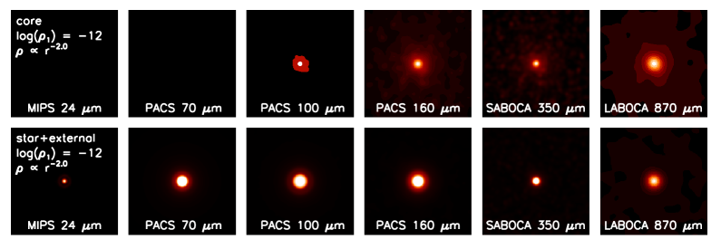
Figure 13.— Convolved model images at the indicated wavelengths, shown on a log scale with the same minimum and maximum flux levels for all panels to illustrate the shape of the model SEDs. Each image is 200^′′ (or 84000 AU) on a side. The top row shows the “core” model images, with log$(\rho_{1})=-12$ and a density profile shape of $\rho\propto r^{-2.0}$, corresponding to the top left panel in Figure 12. The bottom row shows the ”star$+$external” model, with the same density paramaters as the top row, corresponding to the bottom right panel in Figure 12.

6.3. Modified black–body fits to the PBRs

An individual detailed fit to each protostar is beyond the scope of this work considering the vast amount of parameter space needed to model protostellar SEDs (i.e., source luminosity, envelope density, envelope rotation, outflow cavity geometry, external heating, outer envelope structure). Furthermore, unlike most of the HOPS protostars, whose properties can be constrained from a combination of far–IR photometry, 5 µm to 40 µm Spitzer/IRS spectra, and Hubble near–IR imaging (Fischer et al., 2010, 2012), the properties of the SEDs must currently be derived from 5 to 6 photometry points at long wavelength. While the above modeling and analysis shows that the internal source is important, the longer wavelength fluxes are probing the bulk of the envelope mass, expected to mostly be at a single temperature. Furthermore, for density profiles in the range of $\rho(r)\propto r^{-3/2}$ or $r^{-2}$, as assumed above, we expect that most of the envelope will be located at large radii. We therefore perform modified black–body fits to the $\lambda\geq 70$ µm SEDs listed in Tables 4 and 5. For this analysis we use the beam flux measurements for the sub–millimeter 350 µm and 870 µm portion of the SED. The results of the analysis are presented in Table 8 and the model SEDs are plotted with the data in Figure 9.

Before fitting the long–wavelength SEDs of the sources, we apply color corrections to the Herschel 70 µm, 100 µm, and 160 µm fluxes. Following (Launhardt et al., 2012), these photometric color corrections have been derived iteratively from the slopes of the PACS SEDs, using polynomial fits to the values in Table 2 of the PACS calibration release note “PACS Photometer Passbands and Colour Correction Factors for Various Source SEDs” from April 12, 2011. The color corrections for the APEX data are assumed to be negligible.

The form of the modified black–body function is given by

$$S_{\nu}=\Omega\,B_{\nu}(\nu,T_{\rm d})\,(1-e^{-\tau(\nu)}),$$ (2)

where $\Omega$ is the solid angle of the emitting element, $B_{\nu}(T_{\rm d})$ is the Planck function at a dust temperature $T_{\rm d}$, and $\tau(\nu)$ is the optical depth at frequency $\nu$. Here, the optical depth is given by $\tau(\nu)=N_{\rm H}\,m_{\rm H}\,R_{gd}^{-1}\,\kappa(\nu)$, where $N_{\rm H}=2\,\times\,N({\rm H_{2}})+N({\rm H})$ is the total hydrogen column density, $m_{\rm H}$ in the proton mass, $\kappa_{\nu}$ is the assumed dust opacity law from Ossenkopf & Henning (1994), and $R_{gd}$ is the gas–to–dust ratio, assumed to be 110 (Sodroski et al., 1997). The best–fit total masses M_tot reported in Table 8 have been multiplied by an additional factor of 1.36 to account for helium and metals. Furthermore, in Table 8 we also report the peak wavelength of the best–fit modified black–body model. Finally, we estimate L_smm from the model SED, where L_smm is integrated over $\lambda\geq 350~{}\micron$.

If a given source SED has coverage over fewer than 4 long–wavelength points, we do not fit a model to the SED. While all the PBRs sources satisfy this criterion, all the new candidate protostars and HOPS sources do not (see § 5.2) and are therefore not fitted. The errors on $T_{\rm d}$, M_tot, and the thermal component of the luminosity (L_MBB) are estimated through a straight–forward Monte Carlo method. For each source we generate 2000 synthetic SEDs drawn from a normal density with mean and standard deviation equal to those of the measured SED at each wavelength. We then fit each synthetic SED. The reported error is equal to the standard deviation of the resulting distribution of each parameter. These errors do not include systematics introduced by, e.g., our dust model assumption or variation in the gas–to–dust ratio.

We show the modified black–body fit results, along with the SEDs of the PBRs, in Figure 9. The resulting best–fit mass, luminosity, and temperature is also indicated for each source. The model fits the data surprising well considering that significant temperature gradients in the envelope are expected. Furthermore, in all cases the 24 µm point, when detected, has a much higher flux level than the modified black–body model. We interpret this discrepancy as strong evidence for internal heating by a protostar.

Excluding the 70 µm point and fitting only the $\lambda\geq 100$ µm SED has a minor effect on the resulting parameter values. Without 70 µm, the masses systematically increase by 40%, the temperatures decrease by 5%, and the luminosities decrease by 7%. This small effect may be understood by the fact that the 100 µm fluxes are well–correlated with the 70 µm fluxes for this sample, tracing similar material near the protostars. The temperatures at 100 µm and 70 µm are not dramatically different, and most likely both points are dominated by optical–depth effects such that the $\tau=2/3$ surface is not significantly different between the two wavelengths. From Hartmann (2009), the radius of the $\tau=2/3$ surface can be roughly approximated as $r_{\lambda}\propto\kappa_{\lambda}^{2}$; this relation implies that $r_{70}/r_{100}\sim 2.5$.

Our best–fit modified black–body model always underestimates the observed 870 µm flux of all sources. The model sub–millimeter SEDs are always bluer than the observed SEDs. We find that the discrepancy is at the $0.83\pm 0.26$ Jy level (or a factor of $\sim\,3)$ excess), where the error bar represents the standard deviation in the residual distribution. It is likely that this discrepancy is dominated by the larger beam size of the 870 µm observations which has the effect of mixing the source flux with that of the surrounding cold and possibly high–column environment. Contamination to the 870 µm flux by disk emission may also increase this discrepancy. Jørgensen et al. (2009) find average disk masses of $\sim\,0.13$ $\hbox{M}_{\odot}$ (with a large scatter) across their sample of Class 0 sources. The sources in their sample that are comparable to our PBRs, however, are those with the lowest values of T_bol. For reference, they found that IRAS4A1, with a T${}_{bol}=43$ K, has the largest disk mass of 0.46 $\hbox{M}_{\odot}$ in their sample; on the other hand, L1157, with a similar T${}_{bol}=42$ K, has a disk mass about a factor of 4 smaller. We estimate that a 30 K disk of 0.5 $\hbox{M}_{\odot}$ would contribute $\sim\,0.6$ Jy to the beam flux at 870 µm (assuming Ossenkopf & Henning (1994) dust opacities, as above). Therefore, disk emission could indeed contribute to the observed 870 µm flux but further detailed observations at high resolution are needed to disentangle the envelope component from the possible disk emission. Another possible source of ambiguity in interpreting the 870 µm flux discrepancy is the model dust opacity assumption. Furthermore, we do not find an 870 µm discrepancy in the analysis of model images presented in the previous section. This indicates that large disk masses may not be necessary to explain the sub–millimeter fluxes. We therefore emphasize that the disk masses inferred here from the 870 µm excess should be regarded only as upper limits; further detailed investigation into the disk properties of our sources is deferred to future work.

Independent of these issues, it is clear that a more accurate treatment of the data would require all images to be convolved to a matched resolution; however, this approach would have the effect of causing non–detections for a majority of sources at the shorter wavelengths due to the relatively large limiting beam size of our data–set ($\sim 19\arcsec$ at 870 µm). Homogeneously extracted SEDs are therefore not feasible for this data–set as a whole. Nevertheless, we test the effects of convolving the the data before extracting the SEDs. We choose PBRs 119019 as a test source because it is isolated and has approximately median values for the best–fit modified black–body temperature, luminosity, and mass. Ignoring the 870 µm data, this source is clearly detected at 70 µm, 100 µm, 160 µm, and 350 µm. For these four wavelengths, the largest beam size of $\sim 12\arcsec$ corresponds to the 160 µm data. We therefore convolve the 70 µm, 100 µm, and 350 µm data to a resolution matching the 160 µm observations and extract a beam–smoothed SED. We then fit this SED in the same way as described above. Compared to the non–convolved SED modified black–body fitting results, we find that the temperature decreases by $\sim\,4$%, the luminosity increases by $\sim\,10$%, and the the mass in the thermal component increases by $\sim\,30$%. These systematic shifts are similar to but somewhat larger than the errors quoted in Table 8 ($\sim\,2$% on the temperature, $\sim\,10$% on the luminosity, and $\sim\,30$% on the mass). We note, however, that the errors quoted in Table 8 are purely random and do not include any systematic component. We therefore conclude that extracting SEDs from images matched to a resolution of $\sim 12\arcsec$ will not greatly affect our results.

Modified black–body fits provide a somewhat limited means of analysis of our sources since the model assumes a single temperature and density along the line of sight for the emitting material. We expect that the assumption of a single line–of–sight temperature will cause an underestimate of the source masses (e,g., Nielbock et al., 2012; Launhardt et al., 2012). However, radiative transfer models have large ambiguities in the assumed source temperature and density structure, leading to mass estimates that strongly model–dependent. Furthermore, the dust law that is assumed will introduce significant uncertainties into the derived masses, irrespective of the analysis method that is implemented. For example, the masses listed in Table 8 increase by a factor of $\sim\!$4 on average when we assume Draine & Lee (1984) $R_{V}=3.1$ ISM–like dust. These issues indicate that the masses derived here represent lower limits to the true envelope masses. Nevertheless, we consider the modified black–body fits to the measured photometry to provide the most robust estimates of the mass that we currently have.

We note that with only 5 SED flux points at best, fitting a multiple component (modified) black–body model cannot be justified. Since most of the mass is located at relatively large scales and expected to have cold temperatures, excluding the warmer shorter wavelength data arising from inner material will not significantly increase the masses we derive. The modified black–body fits thus to provide an approximate measurement of the optical–depth averaged gross properties of the envelopes being investigated. These issues point to the need for a more sophisticated modeling approach that will be carried out in future work.

7. Discussion

As seen in Figure 11, the observed $70/24$ colors of a protostar can be driven towards redder values through various strongly degenerate parameters. For example, the total column of material along the line–of–sight (LOS) towards a given protostar can have multiple contributions: the attenuation of the mid–IR emission by dense foreground material, the density of the envelope, the amount of envelope flattening, the opening angle of the outflow cavity, and the source inclination. Furthermore, the assumed model central protostar mass remains largely unconstrained by observations to date and can affect the interpretation of the $70/24$ colors.

Foreground extinction can have various contributions, such as intervening dust between the observer and the cloud and dense material associated with the cloud itself, such as filamentary material. Of these two components, the first is expected to be relatively small, while the latter can be expected to vary from source to source by relatively large amounts, with a corresponding effect on the observed colors. For example, some PBRs are located in filamentary regions (e.g., Figures 7 and 8), while others appear more isolated (e.g., see Appendix for Figure 20). We have estimated the effects of foreground extinction levels up to a level of $A_{\rm V}=40$ mag, and find that the values of L_bol, L_smm, and T_bol not significantly affected.

On the other hand, the effects of source inclination are not as straightforward to assess. When considering the presence of flattened rotating envelopes, disks, and outflow cavities, the source inclination will have a large effect on the observed source SED, as illustrated by the model tracks shown in Figure 11 (see also, e.g., Whitney et al., 2003a; De Buizer et al., 2005; Offner et al., 2012).

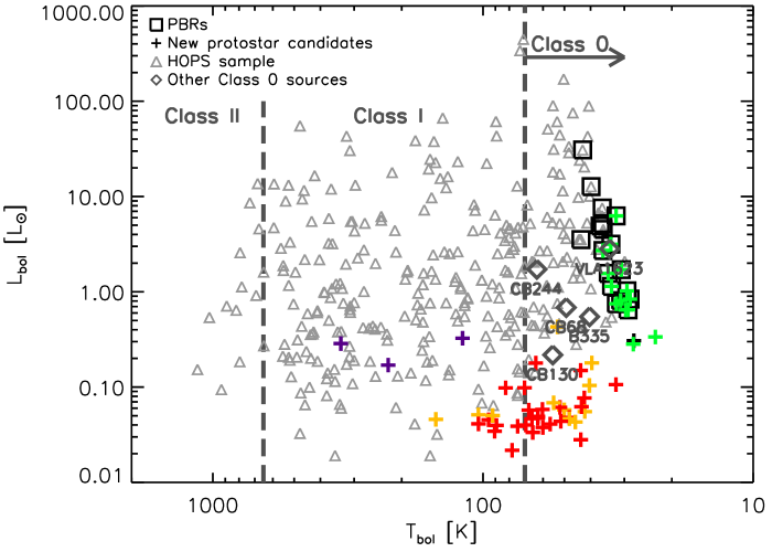
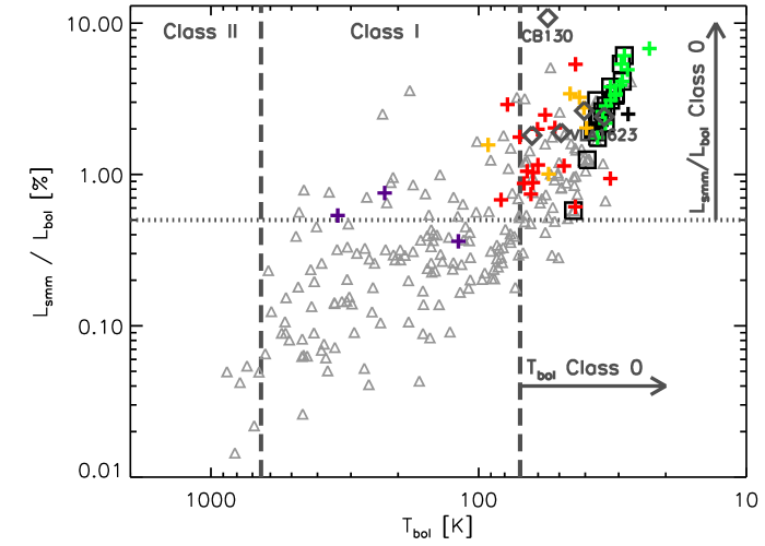
Figure 14.— Left: Bolometric luminosity vs. bolometric temperature for the new candidate protostars ($+$–symbols) and the HOPS protostars (light–grey triangles). The squares indicate the PBRs sample, drawn from both the new candidate protostar sample and the HOPS protostar sample. The dashed lines indicate the canonical T_bol divisions between protostellar Classes. Right: L_smm/L_bol vs bolometric temperature for the subset of sources shown in the left panel for which we have sufficient submillimeter coverage to estimate L_smm (see text). The horizontal dotted line indicates the André et al. (2000) proposed L_smm/L${}_{\rm bol}>0.5$% Class 0 threshold.

Therefore, it appears that the very red PBRs can be explained by multiple effects that all result in increasingly red observed $70/24$ colors. These very red colors may be driven by elevated envelope densities (or equivalently, $\dot{M}_{\rm env}$), high source inclinations, or elevated levels of extinction associated with structures larger than the envelope–protostar system. The current data and SED coverage do not allow us to break these degeneracies conclusively. Furthermore, we consider it likely that the red observed colors are not driven any single cause, but instead are the result of several.

We have, however, designed our PBRs selection to find the densest envelopes in Orion (c.f., Figure 11). Furthermore, the effect of external foreground extinction is not expected to be large at these long wavelengths, even with elevated levels of material along the LOS (see above). Indeed, we have also shown that the PBRs require a central heating source, indicating that the detection of a 70 µm point source drives the interpretation of the sample as Class 0 sources, irrespective of source inclination. However, we note that if the central masses are significantly different than the assumed value of 0.5 $\hbox{M}_{\odot}$, then for a fixed reference envelope density the inferred envelope infall rates need to be scaled accordingly (see Equation 1).

To further investigate the evolutionary state of the PBRs, in Figure 14 we show we the values of L_bol, T_bol, and L_smm$/$L_bolfor the entire sample of new candidate protostars and the previously identified Spitzer HOPS sample (Fischer et al. in preparation). In the left panel, we show L_bol vs. T_bol for the entire sample of new protostar candidates, including those flagged as possible extra–galactic contamination. We also show the four reference Class 0 sources presented in Table 8. The PBRs sample in particular, and the entire sample of new candidate protostars, are generally clustered around low T_bol values. Ignoring inclination degeneracies and other considerations, these low T_bolvalues indicate that the PBRs sample is indeed composed of young Class 0 sources. In the right panel, we show T_bol vs. L_smm/L_bol for the sources with sufficient coverage to estimate L_smm (see § 6.2). The PBRs, as expected if the sample can be explained as Class 0 sources, cluster around larger values of L_smm/L_bol compared to the rest of the sample. André et al. (2000) proposed the L_smm/L${}_{\rm bol}>0.5\%$ threshold for Class 0 sources, and all but one of the new candidate protostars for which we can estimate L_smm fall into this category. Irrespective of the evolutionary indicator that is chosen (T_bol or L_smm/L_bol ), all of the new candidate protostars in both the reliable and lower probability categories (green and yellow points, respectively), would be considered of Class 0 status. Finally, while the PBRs $70/24>1.65$ color criterion causes some sources with very low values of T_bol and very high values of L_smm/L_bol to be missed, the color selection is able to capture the vast majority of the most extreme Class 0 sources at the extrema of the L_smm/L_bol and T_bol distributions.

This evidence strongly supports the interpretation of the PBRs (and indeed all the sources classified as reliable protostellar candidates) as very dense Class 0 protostars, irrespective of the source inclination. On the other hand, the new candidate protostar sample, taken as a whole, may be explained by a combination of the effects described above: high inclination, high densities, and extreme values of foreground extinction, along with elevated levels of extragalactic contamination. Of particular interest is the possibility that some of the sources classified as low probability protostars at low L_bol values may be confirmed as bona fide protostars with future observations (see Offner & McKee, 2011, for a detailed discussion of the significance of such sources); this will be investigated in future work (Stutz et al. in preparation).

To definitely measure the inclinations of our sample of sources and to therefore determine envelope densities more accurately we require millimeter line emission maps at high resolution from e.g., ALMA, along with single dish observations of high density tracers. A vigorous follow–up campaign is therefore underway to more firmly place these protostars within the context of star formation in the Orion clouds. We are observing ammonia spectra toward the full sample of protostar candidates to verify the presence of dense molecular gas and determine kinetic temperatures. A Herschel PACS range spectroscopy program toward 8 PBRs will characterize the energetics of outflows and UV heating on small–scales. The outflows (CO), dust continuum, and surrounding dense molecular gas (N₂H⁺) are being observed in the millimeter to determine the source inclinations, outflow opening angles, inner envelope properties, and the kinematics of the larger–scale dense gas.

8. Conclusions

We have discovered a sample of 55 new candidate protostars in Orion with Herschel, as part of the HOPS Open Time Key Programme scan–map observations at 70 µm and 160 µm. We conclude that:

$\bullet$ The new candidate protostars are either very faint or undetected at Spitzer wavelengths. We find 34 sources with 24 µm magnitudes that are greater than 7.0 and 21 sources that are undetected in the MIPS 24 µm band.

$\bullet$ We analyze the IRAC colors and the broad shape of the SEDs between 3.6 µm and 160 µm. Based on this analysis, we classify the sample as follows: 27% (15 sources) are considered reliable protostars, 18% (10 sources) are considered lower probability protostars, 47% (26 sources) are classified as extragalactic contamination, including AGN, 3 sources have IRAC colors consistent with stellar photospheres but Herschel and APEX SEDs consistent with cold dust emission, and 1 source does not have IRAC coverage. We find that the subset of sources without 24 µm detections dominates the number of sources categorized as most reliable protostellar candidates by a factor of $\sim\,3$, suggesting that sources with no short–wavelength detections and only PACS 70 µm and longer wavelength detections are much less likely to be of extragalactic origin.

$\bullet$ We combine the new protostar candidate sample with the previously identified Spitzer HOPS sample and find that 18 sources have $70/24$ colors greater than 1.65. These are the reddest protostars known in Orion, 11 of which are newly identified Herschel sources in the reliable protostar category listed above. We name these sources “PACS Bright Red sources”, or PBRs. Compared to the other protostars in the HOPS fields, the PBRs populate the extrema in the distributions of standard evolutionary diagnostics, having both the largest L_smm/L_bol ratios and lowest T_bol values. The PBR source SEDs and peak SED wavelengths are consistent with the hypothesis that the PBRs do indeed represent a population composed of Class 0 sources with the densest envelopes in Orion.

$\bullet$ A comparison to radiative transfer models of rotating, collapsing protostellar envelopes with outflow cavities show that the $70/24>1.65$ color limit selects sources with envelope densities with log $\rho_{1}/({\rm g\,cm}^{-3})\gtrsim-13.4$, irrespective of inclination effects. While the $70/24>1.65$ color selects sources with dense envelopes, this color criterion does not find all dense sources above the threshold of of $\rho_{1}/({\rm g\,cm}^{-3})=-13.4$. Therefore this selection should be used in conjunction with other evolutionary indicators, namely millimeter and sub–millimeter measurements, to determine the nature of the observed sources.

$\bullet$ Our modeling of the PBRs SEDs reveals that these sources are not consistent with being externally heated starless cores; the presence of a 70 µm point source requires that the sample be interpreted as dense envelopes containing embedded protostars.

$\bullet$ The fraction of known protostars that are PBRs varies from 1% in the Orion A cloud to 17% in the Orion B cloud, with an an average fraction over the Orion complex of 5%. These numbers suggest that if the PBRs represent a distinct phase in protostellar evolutions, protostars spend on average 5% of their lifetime in the PBRs phase. Most of the PBRs in the Orion B cloud are concentrated in dense gas near the NGC2068, NGC2071, and NGC2023 nebulae. These regions of dense gas are also known for a lack of more evolved pre–main sequence stars. The high percentage of PBRs in Orion B suggests either that the regions containing the PBRs may currently be undergoing more vigorous star–formation than other regions of Orion, or that the PBRs lifetime is longer in these regions.

$\bullet$ The sources with $70/24<1.65$ colors and faint 70 µm fluxes must be confirmed as either protostellar or contamination sources before their significance can be assessed. If confirmed as the former, however, this sample would constitute an important population of very low–luminosity, cold protostars previously unobserved, most interesting from the point of view of constraining the faint end of the luminosity function of protostars.

$\bullet$ We expect that a comparable number of very red protostars will be found with Herschel in more near–by star–forming regions. We caution that a careful treatment of possible extragalactic contamination must be implemented to understand the broader significance of such sources.

Appendix A Previous PBRs detections

We searched the SIMBAD and VizieR (Ochsenbein et al., 2000) services for previous identifications of the PBRs. We restricted our search to a radius of 20$\arcsec$ from the 70 µm source coordinates. The results are summarized in Table 6. This list is likely incomplete and is intended to provide a resource and rough guide to some of the previous detections of these sources.

$-$ 061012, 119019, and 097002: None found.

$-$ HOPS169: Known protostar and outflow bipolar outflow V380 Ori NE (e.g., Davis et al., 2000). Stanke et al. (2002) detected source 59 in their 2.12 µm catalog of Orion A, offset by 6$\arcsec$ from our source coordinates. Davis et al. (2009) also detected an outflow about 2$\arcsec$ away from our coordinates. Nutter & Ward-Thompson (2007) classified this source as hosting a young stellar object (YSO) and measured an 850 µm–flux–derived mass of 2.8 $\hbox{M}_{\odot}$ (assuming a temperature of 20 K and a distance of 400 pc).

$-$ 019003: Since this source is located in the very crowded and complex ONC filament, it is often not clear which previous identifications may be associated with it in particular. Tsujimoto et al. (2003) listed a near–IR source located 3.35$\arcsec$ away from our coordinates. Nutter & Ward-Thompson (2007) detected a source offset by 8.4$\arcsec$; they classified it as hosting a YSO and measure a mass of 6.2 $\hbox{M}_{\odot}$. While it is not clear if the detection is associated with the PBRs we consider it probable. Chini et al. (1997) and Nielbock et al. (2003) likely detected this source in their 1.3 mm maps near FIR1a in OMC–2, although their beam sizes were too large identify the source unambiguously.

$-$ 082005: This source was previously classified as a starless core (e.g., Johnstone & Bally, 2006; Nutter & Ward-Thompson, 2007; Mookerjea et al., 2009). The Nutter & Ward-Thompson (2007) location of the source is about 8$\arcsec$ away from our source with an associated mass of 3.3 $\hbox{M}_{\odot}$. Mookerjea et al. (2009) measured a mass of 4.3 $\hbox{M}_{\odot}$ for this source.

$-$ HOPS372 and 082012: These sources have coordinates that are significantly offset from the Nutter & Ward-Thompson (2007) coordinates; the two sources are unresolved and lie about 13$\arcsec$ away from their catalog entree, with a mass of 12.7 $\hbox{M}_{\odot}$. The Mookerjea et al. (2009) analysis derived a mass of 1 $\hbox{M}_{\odot}$ for 082012 (MM1) and 7.4 $\hbox{M}_{\odot}$ for HOPS372 (MM2), from modified black–body fits to long–wavelength SEDs.

$-$ 090003: Miettinen et al. (2009) detected this source (SMM3) in their 850 µm map, and concluded that it is a promising Class 0 candidate based on the shape of the SED. They calculated a mass of about 7.5 $\hbox{M}_{\odot}$ for this source. Miettinen et al. (2010) and Miettinen et al. (2012) also observed this source in various molecular line transitions and with SABOCA at 350 µm; their measured flux for this source is $S^{peak}_{350}=3.63$ Jy beam^-1. We include their flux measurement and the 350 µm map in our analysis.

$-$ HOPS358: Strom et al. (1976), Strom et al. (1986), and (Reipurth et al., 1999) detected the Herbig–Haro complex HH24–26, with HH25 located about 10$\arcsec$ away from HOPS358. This source is also included in the Wu et al. (2004) high velocity outflow catalog. Nutter & Ward-Thompson (2007) classified a nearby source (11$\arcsec$ away) as a starless core with a mass of 6.3 $\hbox{M}_{\odot}$.

$-$ 091015 and 091016: These sources were detected by Lis et al. (e.g., 1999) at 1.3 mm and 350 µm (as sources 5 and 6). The reported masses are $\sim\!2$ $\hbox{M}_{\odot}$ for each source. Both sources are classified as starless by Nutter & Ward-Thompson (2007), with catalog masses of 0.8 $\hbox{M}_{\odot}$ (091015) and 1.3 $\hbox{M}_{\odot}$ (091016).

$-$ HOPS373 and 093005: Both sources were classified as starless by Nutter & Ward-Thompson (2007), with reported masses of 4.2 $\hbox{M}_{\odot}$ (HOPS373) and 3.9 $\hbox{M}_{\odot}$ (093005). Motte et al. (2001) observed this region at 450 and 850 µm and also classified 093005 as a starless core, based on the lack of evidence for an embedded source. Source HOPS373, on the other hand, is known to be driving a CO outflow (Gibb & Little, 2000), and therefore has been classified as a candidate Class 0 source. Furthermore, Haschick et al. (1983) identified a water maser near the HOPS373 location.

$-$ 302002: Nutter & Ward-Thompson (2007) reported a mass of 2.7 $\hbox{M}_{\odot}$ and classified this source as protostellar. Phillips et al. (2001) classify this source (LBS18S) as pre–protostellar, however.

$-$ HOPS359: Nutter & Ward-Thompson (2007) classified this source as protostellar and measure a mass of 2.7 $\hbox{M}_{\odot}$.

$-$ HOPS341: This source is strongly blended with HOPS340. We have listed some detections of the combined system in Table 6.

$-$ HOPS354: Reipurth et al. (2008) described this source in the context of the L1622 cloud. Bally et al. (2009) also detected this source in their analysis of Spitzer IRAC images but did not analyze it in detail.

Appendix B Gallery of images of PACS Bright Red sources

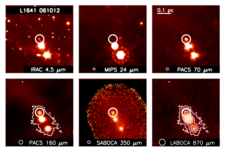
Figure 15.— Same as Figure 7, showing $4\arcmin\times 4\arcmin$ images of PBRs 061012. The IRAC–band emission associated with the source is clearly visible at 4.5 µm. Contours indicate the 870 µm emission levels at {0.1, 0.25, 0.4, 0.55, 0.7} Jy beam^-1; the long wavelength sum–mm data trace the cold envelope material associated with the source. The 160 µm panel is shown with the lowest 870 µm emission contour.

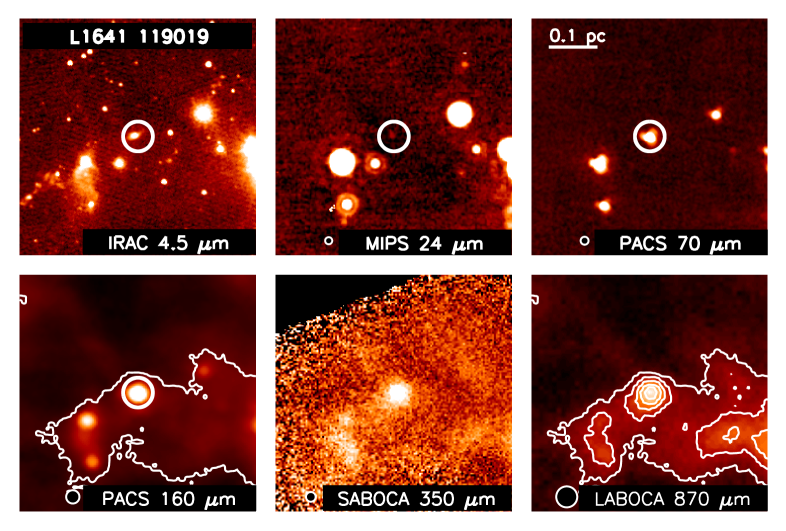
Figure 16.— Same as Figure 7, showing $4\arcmin\times 4\arcmin$ images and SED of PBRs 119019. Contours indicate the 870 µm emission levels at {0.1, 0.2, 0.3, 0.4, 0.5} Jy beam^-1. This source has prominent IRAC emission and is located in an IRAC 8 µm and MIPS 24 µm shadow.

Figure 17.— Same as Figure 7, showing $4\arcmin\times 4\arcmin$ images and SED of HOPS169. Contours indicate the 870 µm emission levels at {0.1, 0.2, 0.4, 0.6, 0.8} Jy beam^-1. This source has clear outflow activity, traced by the IRAC emission, and appears to be at high inclination.

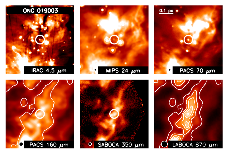
Figure 18.— Same as Figure 7, showing $4\arcmin\times 4\arcmin$ images and SED of PBR source 019003. Contours indicate the 870 µm emission levels at {0.5, 1.0, 1.5, 2.0, 2.5} Jy beam^-1. This source has indications outflow activity, as traced by the IRAC emission. The Herschel photometry may be strongly affected by blending due to the source location in a very dense filament.

Figure 19.— Top: Same as Figure 7, showing $5\arcmin\times 5\arcmin$ images of three red sources: HOPS372 and 082012 (top) and 082005 (bottom). Contours indicate the 870 µm emission levels at {0.25, 0.5, 0.75, 1.0, 1.25, 1.5} Jy beam^-1. No IRAC emission is detected for 082005; however, this source is located in dense filamentary material traced by the sub-mm emission and an 8 µm absorption feature.

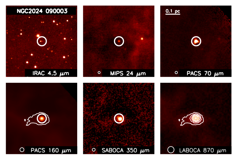
Figure 20.— Same as Figure 7, showing $4\arcmin\times 4\arcmin$ images and SED of PBRs 090003. Contours indicate the 870 µm emission levels at {0.25, 0.5, 0.75, 1.0, 1.25, 1.5} Jy beam^-1. The IRAC data show faint indications of extended emission, possibly associated with an outflow activity or a second source. The 350 µm image and SED point are from Miettinen et al. (2012)

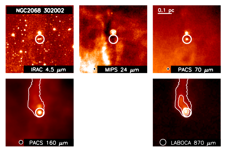
Figure 21.— Same as Figure 7; $4\arcmin\times 4\arcmin$ images of PBRs 302002. Contours indicate the 870 µm emission levels at {0.25, 0.5, 0.75, 1.0, 1.25, 1.5} Jy beam^-1, tracing the cometary globule shaped region. The IRAC data show indications of emission associated with outflow activity; furthermore, the 4.5 µm data show evidence that this source is observed at high inclination. This source is the second most massive source in our sample, with a best–fit M${}_{env}=1.7$ $\hbox{M}_{\odot}$.

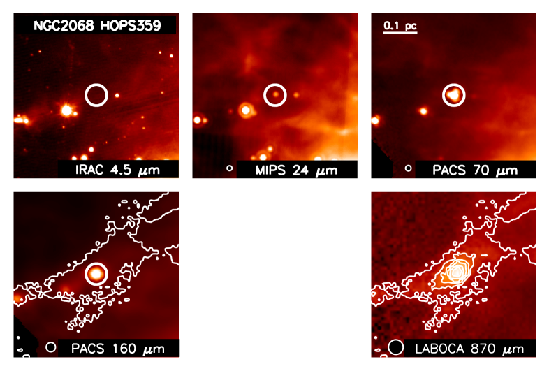
Figure 22.— Same as Figure 7; $4\arcmin\times 4\arcmin$ images of HOPS359. Contours indicate the 870 µm emission levels at {0.25, 0.5, 0.75, 1.0, 1.25, 1.5} Jy beam^-1.

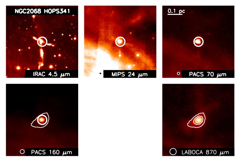
Figure 23.— Same as Figure 7; $4\arcmin\times 4\arcmin$ images of HOPS341. Contours indicate the 870 µm emission levels at {0.25, 0.5, 0.75, 1.0} Jy beam^-1. The $\times$–shaped morphology of this source in the IRAC bands indicated that tit is a binary. Indeed, the photometry of this source is strongly blended with HOPS340; nevertheless we include this source in our sample for completeness.

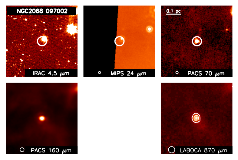
Figure 24.— Same as Figure 7; $4\arcmin\times 4\arcmin$ images of PBRs 097002. Contours indicate the 870 µm emission levels at {0.25, 0.5} Jy beam^-1.

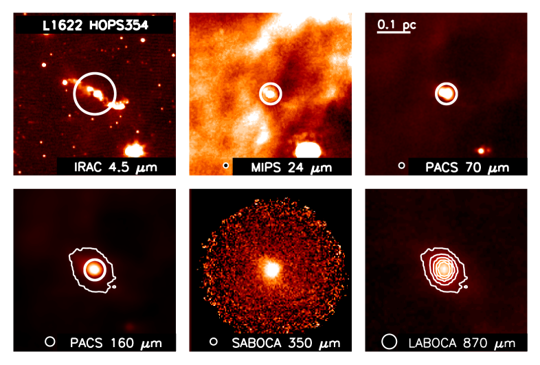
Figure 25.— Same as Figure 7; $4\arcmin\times 4\arcmin$ images of HOPS354. Contours indicate the 870 µm emission levels at {0.25, 0.5, 0.75, 1.0, 1.25} Jy beam^-1. The IRAC images display clear indications of outflow activity; furthermore the source appears highly inclined.

Table 1Summary of HOPS Herschel PACS L1641 observations

HOPS	R.A.a	Decl.a	Field	AOR ID	OD	Map size
group name	h:m:s	∘:$\arcmin$;$\arcsec$				$\arcmin\times\arcmin$
54	5:42:38.570	$-$8:50:18.67	L1641	1342218796(7)	704	8$\times$8
53	5:43:06.770	$-$8:46:09.56	L1641	1342218735(6)	703	8$\times$8
60	5:41:29.690	$-$8:41:28.59	L1641	1342215359(60)	662	8$\times$8
55	5:42:50.490	$-$8:40:54.73	L1641	1342218798(9)	704	8$\times$8
56	5:42:52.750	$-$8:37:20.98	L1641	1342205256(7)	502	8$\times$8
117	5:41:33.250	$-$8:36:41.62	L1641	1342218790(1)	704	8$\times$8
59	5:42:55.540	$-$8:32:48.26	L1641	1342218794(5)	704	8$\times$8
58	5:43:09.580	$-$8:29:27.13	L1641	1342218788(9)	704	8$\times$8
61	5:42:47.760	$-$8:16:50.72	L1641	1342205254(5)	502	8$\times$8
67	5:40:20.130	$-$8:14:05.78	L1641	1342227078(9)	831	8$\times$8
119	5:40:47.820	$-$8:10:28.38	L1641	1342206322(3)	516	8$\times$8
62	5:42:47.370	$-$8:10:08.76	L1641	1342218792(3)	704	8$\times$8
63	5:41:35.440	$-$8:08:22.49	L1641	1342218800(1)	704	8$\times$8
66	5:40:54.500	$-$8:06:08.98	L1641	1342215361(2)	662	8$\times$8
118	5:41:27.790	$-$8:04:03.70	L1641	1342205250(1)	502	8$\times$8
78	5:38:51.480	$-$8:01:27.44	L1641	1342228169(70)	844	5$\times$5
64	5:41:49.950	$-$8:01:26.51	L1641	1342205252(3)	502	5$\times$5
69	5:40:38.330	$-$8:00:36.00	L1641	1342227080(1)	831	5$\times$5
65	5:41:24.880	$-$8:00:02.34	L1641	1342215591(2)	663	8$\times$8
72	5:40:20.710	$-$7:56:01.36	L1641	1342218733(4)	703	8$\times$8
70	5:40:40.530	$-$7:54:39.82	L1641	1342228167(8)	844	5$\times$5
121	5:41:23.440	$-$7:54:39.26	L1641	1342205248(9)	502	8$\times$8
68	5:41:19.660	$-$7:50:41.03	L1641	1342227848(9)	842	5$\times$5
74	5:40:17.690	$-$7:49:29.88	L1641	1342218731(2)	703	8$\times$8
71	5:40:40.150	$-$7:49:18.71	L1641	1342228163(4)	844	8$\times$8
320	5:40:58.890	$-$7:48:02.05	L1641	1342228165(6)	844	5$\times$5
73	5:40:42.910	$-$7:45:01.91	L1641	1342228425(6)	847	5$\times$5
75	5:40:24.620	$-$7:43:08.26	L1641	1342227082(3)	831	5$\times$5
76	5:40:26.090	$-$7:37:32.02	L1641	1342205246(7)	502	5$\times$5
79	5:39:57.200	$-$7:30:19.89	L1641	1342205244(5)	502	8$\times$8
77	5:40:44.670	$-$7:29:54.46	L1641	1342228427(8)	847	5$\times$5
123	5:40:08.780	$-$7:27:27.68	L1641	1342228161(2)	844	5$\times$5
26	5:39:24.640	$-$7:26:13.81	L1641	1342218729(30)	703	8$\times$8
25	5:39:56.200	$-$7:24:53.71	L1641	1342215589(90)	663	8$\times$8
313	5:39:33.300	$-$7:22:57.36	L1641	1342227084(5)	831	5$\times$5
28	5:38:56.470	$-$7:20:44.32	L1641	1342227086(7)	831	8$\times$8
30	5:38:44.050	$-$7:11:49.89	L1641	1342204254(5)	484	8$\times$8
29	5:39:06.710	$-$7:11:12.80	L1641	1342204252(3)	484	8$\times$8
32	5:38:01.100	$-$7:07:37.01	L1641	1342227045(6)	830	8$\times$8
312	5:38:46.540	$-$7:05:37.46	L1641	1342205242(3)	502	5$\times$5
31	5:38:44.870	$-$7:00:37.03	L1641	1342204256(7)	484	8$\times$8
33	5:38:20.090	$-$6:59:04.85	L1641	1342228171(2)	844	5$\times$5
35	5:37:24.460	$-$6:58:32.77	L1641	1342227314(5)	833	5$\times$5
34	5:37:59.990	$-$6:57:27.50	L1641	1342205240(1)	502	8$\times$8
101	5:37:17.090	$-$6:49:49.33	L1641	1342227312(3)	833	5$\times$5
36	5:37:52.390	$-$6:47:18.67	L1641	1342227088(9)	831	8$\times$8
38	5:36:22.050	$-$6:45:41.23	L1641	1342205238(9)	502	8$\times$8
40	5:36:26.650	$-$6:38:27.74	L1641	1342227094(5)	831	8$\times$8
37	5:37:17.280	$-$6:36:18.18	L1641	1342227090(1)	831	8$\times$8
43	5:35:50.020	$-$6:34:53.40	L1641	1342227310(1)	833	5$\times$5
50	5:34:15.880	$-$6:34:32.70	L1641	1342217748(9)	686	8$\times$8
39	5:36:41.330	$-$6:34:00.08	L1641	1342227092(3)	831	5$\times$5
41	5:36:19.440	$-$6:29:06.79	L1641	1342227316(7)	833	5$\times$5
45	5:35:34.120	$-$6:26:41.70	L1641	1342215593(4)	663	8$\times$8
311	5:34:39.860	$-$6:25:14.16	L1641	1342203649(50)	470	5$\times$5
42	5:36:22.460	$-$6:23:39.14	L1641	1342205236(7)	502	8$\times$8
44	5:36:36.980	$-$6:14:57.98	L1641	1342204258(9)	484	5$\times$5
51	5:35:22.180	$-$6:13:06.24	L1641	1342227318(9)	833	5$\times$5
47	5:36:17.260	$-$6:11:11.00	L1641	1342227324(5)	833	5$\times$5
49	5:35:52.000	$-$6:10:01.85	L1641	1342227322(3)	833	5$\times$5
52	5:35:33.210	$-$6:06:09.65	L1641	1342227320(1)	833	5$\times$5
48	5:36:31.360	$-$6:01:16.81	L1641	1342217444(5)	685	8$\times$8
5	5:35:07.960	$-$5:56:56.40	L1641	1342204248(9)	484	8$\times$8
6	5:35:24.560	$-$5:55:33.42	L1641	1342227328(9)	833	5$\times$5
7	5:36:19.020	$-$5:55:25.46	L1641	1342227326(7)	833	5$\times$5
8	5:35:04.400	$-$5:51:00.76	L1641	1342217446(7)	685	8$\times$8
9	5:33:30.710	$-$5:50:41.03	L1641	1342217750(1)	686	8$\times$8
10	5:36:10.100	$-$5:50:08.34	L1641	1342227096(7)	831	5$\times$5
12	5:34:46.830	$-$5:42:28.72	L1641	1342204246(7)	484	8$\times$8
13	5:35:17.340	$-$5:42:14.51	L1641	1342227098(9)	831	5$\times$5
14	5:34:30.440	$-$5:37:47.44	L1641	1342204244(5)	484	8$\times$8

Table 2Summary of HOPS Herschel PACS ONC, NGC2024, NGC2068, and L1622 observations

HOPS	R.A.a	Decl.a	Region	AOR ID	OD	Map size
group name	h:m:s	∘:$\arcmin$;$\arcsec$				$\arcmin\times\arcmin$
15	5:35:06.620	$-$5:35:05.68	ONC	1342205234(5)	502	8$\times$8
308	5:33:45.870	$-$5:32:58.09	ONC	1342204433(4)	487	5$\times$5
16	5:34:43.990	$-$5:32:11.21	ONC	1342217448(9)	685	8$\times$8
17	5:35:16.320	$-$5:29:32.60	ONC	1342217450(1)	685	8$\times$8
18	5:33:55.730	$-$5:22:39.97	ONC	1342217752(3)	686	8$\times$8
200	5:35:19.270	$-$5:14:46.49	ONC	1342205232(3)	502	8$\times$8
130	5:35:24.710	$-$5:09:06.02	ONC	1342205228(9)	502	8$\times$8
135	5:35:26.280	$-$5:06:35.24	ONC	1342205226(7)	502	8$\times$8
19	5:35:23.300	$-$5:00:35.73	ONC	1342204250(1)	484	8$\times$8
20	5:35:13.770	$-$4:54:57.33	ONC	1342217758(9)	686	8$\times$8
21	5:34:32.340	$-$4:53:54.26	ONC	1342217754(5)	686	8$\times$8
306	5:35:32.280	$-$4:46:48.47	ONC	1342191970(1)	300	5$\times$5
24	5:35:23.340	$-$4:40:10.45	ONC	1342217756(7)	686	8$\times$8
80	5:40:51.710	$-$2:26:48.62	NGC2024	1342226729(30)	826	5$\times$5
81	5:41:28.940	$-$2:23:19.36	NGC2024	1342226733(4)	826	5$\times$5
82	5:41:23.740	$-$2:16:51.10	NGC2024	1342228913(4)	858	8$\times$8
83	5:41:42.180	$-$2:16:26.20	NGC2024	1342227049(50)	830	8$\times$8
85	5:42:02.620	$-$2:07:45.70	NGC2024	1342226735(6)	826	5$\times$5
86	5:41:43.560	$-$1:53:28.42	NGC2024	1342227047(8)	830	8$\times$8
89	5:42:27.680	$-$1:20:01.00	NGC2024	1342205220(1)	502	5$\times$5
90	5:43:04.370	$-$1:16:11.60	NGC2024	1342228376(7)	849	8$\times$8
91	5:46:06.690	$-$0:13:05.15	NGC2068	1342205218(9)	502	8$\times$8
92	5:46:14.210	$-$0:05:26.84	NGC2068	1342205216(7)	502	5$\times$5
93	5:46:40.830	$+$0:00:30.52	NGC2068	1342215363(4)	662	8$\times$8
94	5:46:39.580	$+$0:04:16.61	NGC2068	1342228365(6)	848	5$\times$5
302	5:46:28.320	$+$0:19:49.40	NGC2068	1342228374(5)	849	5$\times$5
303	5:47:24.810	$+$0:20:59.68	NGC2068	1342227966(7)	843	8$\times$8
96	5:47:08.970	$+$0:21:52.86	NGC2068	1342215587(8)	663	8$\times$8
128	5:46:56.220	$+$0:23:42.41	NGC2068	1342218727(8)	703	8$\times$8
301	5:45:53.590	$+$0:25:27.30	NGC2068	1342216450(1)	675	5$\times$5
97	5:47:58.060	$+$0:35:30.12	NGC2068	1342227969(70)	843	8$\times$8
98	5:47:31.850	$+$0:38:05.77	NGC2068	1342227971(2)	843	8$\times$8
300	5:47:42.990	$+$0:40:57.50	NGC2068	1342205214(5)	502	5$\times$5
0	5:54:15.240	$+$1:43:15.59	L1622	1342215365(6)	662	8$\times$8
1	5:54:55.370	$+$1:45:03.08	L1622	1342218780(1)	704	8$\times$8
3	5:54:23.540	$+$1:49:17.78	L1622	1342218703(4)	702	8$\times$8
4	5:54:36.260	$+$1:53:54.00	L1622	1342218778(9)	704	8$\times$8

Note. — Note: the ONC field contains the extended Orion Nebula region, the NGC1977 region, and OMC2/3; the NGC2024 field contains the NGC2024 HII region and the NGC2023 reflection nebula. The NGC2068 field includes the NGC2068 and NGC2071 reflection nebulae as well as LBS23 region.

Table 3Herschel protostar candidate coordinates and photometry

Source	group	R.A.a	Decl.a	Field	$24~{}\micron$	$70~{}\micron$	$160~{}\micron$	flagb	870 $\micron$	Tbol	Lbol
	name	h:m:s	∘:$\arcmin$;$\arcsec$		[mJy]	[mJy]	[mJy]		detectionc	[K]	[L⊙]
061012	061	05:42:48.87	$-$08:16:10.70	L1641	$\leq$1.14	703$\pm$35	5634$\pm$845	1	$\cdots$	32.1$\pm$0.9	0.75$\pm$0.06
119019	119	05:40:58.47	$-$08:05:36.10	L1641	1.46$\pm$0.2	1604$\pm$80.	10745$\pm$1612	1	Yes	34.4$\pm$0.8	1.56$\pm$0.14
026011	026	05:39:17.00	$-$07:24:26.64	L1641	$\leq$1.30	78.4$\pm$3.9	2516$\pm$377	1	Yes	23.0$\pm$1.0	0.34$\pm$0.03
313006	313	05:39:30.75	$-$07:23:59.40	L1641	$\leq$1.25	138$\pm$7.	2198$\pm$330	1	Yes	27.8$\pm$1.0	0.28$\pm$0.03
029003	029	05:39:13.15	$-$07:13:11.69	L1641	1.19$\pm$0.2	29.5$\pm$1.5	365$\pm$55	1	$\cdots$	42.0$\pm$1.5	0.06$\pm$0.01
019003	019	05:35:23.92	$-$05:07:53.46	ONC	$\leq$16.2	2506$\pm$127	31577$\pm$4737	1	Yes	33.6$\pm$1.1	3.16$\pm$0.31
082005	082	05:41:29.40	$-$02:21:17.06	NGC2024	$\leq$3.13	506$\pm$25	9308$\pm$140	1	Yes	29.3$\pm$0.8	1.02$\pm$0.11
082012	082	05:41:24.94	$-$02:18:08.54	NGC2024	6.51$\pm$0.4	4571$\pm$229	51254$\pm$7688	1	Yes	32.2$\pm$0.9	6.27$\pm$0.65
090003	090	05:42:45.23	$-$01:16:14.18	NGC2024	4.74$\pm$0.3	3286$\pm$164	16937$\pm$2541	1	Yes	36.0$\pm$0.8	2.71$\pm$0.24
091015	091	05:46:07.65	$-$00:12:20.73	NGC2068	$\leq$1.29	648$\pm$32	6615$\pm$992	1	Yes	30.9$\pm$0.8	0.81$\pm$0.07
091016	091	05:46:09.97	$-$00:12:16.85	NGC2068	$\leq$1.14	431$\pm$22	5108$\pm$766	1	Yes	29.1$\pm$0.9	0.65$\pm$0.06
093005	093	05:46:27.75	$-$00:00:53.81	NGC2068	$\leq$1.14	1427$\pm$71.	12131$\pm$1820	1	Yes	30.8$\pm$0.9	1.71$\pm$0.15
302002	302	05:46:28.24	00:19:27.00	NGC2068	$\leq$1.14	302$\pm$15	7187$\pm$108	1	Yes	28.6$\pm$0.9	0.84$\pm$0.09
097002	097	05:48:07.76	00:33:50.79	NGC2068	$\leq$1.14	1049$\pm$52.	7993$\pm$120	1	Yes	33.4$\pm$0.9	1.14$\pm$0.11
300001	300	05:47:43.36	00:38:22.43	NGC2068	$\leq$7.19	478$\pm$24	5042$\pm$756	1	Yes	29.6$\pm$0.9	0.65$\pm$0.06
068006	068	05:41:11.79	$-$07:53:35.09	L1641	9.19$\pm$0.2	44.8$\pm$2.2	146$\pm$22	2	$\cdots$	149.7$\pm$5.06	0.05$\pm$0.01
038002	038	05:36:11.11	$-$06:49:11.29	L1641	$\leq$1.25	36.4$\pm$1.8	537$\pm$81	2	$\cdots$	40.4$\pm$1.0	0.10$\pm$0.01
037003	037	05:37:00.35	$-$06:37:10.95	L1641	8.85$\pm$0.2	725$\pm$36	3798$\pm$570	2	$\cdots$	53.1$\pm$1.7	0.43$\pm$0.03
037008	037	05:37:34.31	$-$06:35:20.33	L1641	$\leq$1.39	27.7$\pm$1.4	321$\pm$48	2	$\cdots$	45.5$\pm$1.9	0.04$\pm$0.01
092011	092	05:46:26.17	$-$00:04:45.31	NGC2068	2.31$\pm$0.2	77.8$\pm$3.9	363$\pm$54	2	$\cdots$	104.1$\pm$5.63	0.05$\pm$0.01
093001	093	05:46:56.32	$-$00:03:14.73	NGC2068	$\leq$1.14	21.8$\pm$1.1	217$\pm$33	2	Yes	47.9$\pm$0.7	0.05$\pm$0.01
302004	302	05:46:16.55	00:21:35.09	NGC2068	2.87$\pm$0.2	108$\pm$5.	283$\pm$42	2	$\cdots$	54.8$\pm$1.8	0.07$\pm$0.01
096023	096	05:46:53.23	00:22:10.05	NGC2068	$\leq$2.13	147$\pm$7.	1691$\pm$254	2	$\cdots$	39.6$\pm$1.4	0.18$\pm$0.02
301003	301	05:46:02.15	00:23:29.86	NGC2068	8.08$\pm$0.2	42.6$\pm$2.1	231$\pm$35	2	$\cdots$	92.1$\pm$3.8	0.05$\pm$0.01
000011	000	05:54:32.10	01:42:54.92	L1622	$\leq$1.25	28.5$\pm$1.4	147$\pm$22	2	$\cdots$	50.1$\pm$0.5	0.06$\pm$0.01
053002	053	05:43:24.07	$-$08:49:03.75	kOri	$\leq$1.38	33.5$\pm$1.7	190$\pm$28	3	$\cdots$	43.2$\pm$0.3	0.06$\pm$0.01
117004	117	05:41:40.40	$-$08:41:40.60	L1641	1.17$\pm$0.2	25.3$\pm$1.3	234$\pm$35	3	$\cdots$	56.4$\pm$2.2	0.04$\pm$0.01
117014	117	05:41:29.28	$-$08:36:14.60	L1641	1.20$\pm$0.2	31.0$\pm$1.6	237$\pm$36	3	$\cdots$	32.2$\pm$2.4	0.11$\pm$0.01
119016	119	05:40:40.54	$-$08:05:55.00	L1641	1.97$\pm$0.2	42.7$\pm$2.1	148$\pm$22	3	$\cdots$	62.7$\pm$1.7	0.05$\pm$0.01
121011	121	05:41:37.90	$-$07:55:44.35	L1641	1.46$\pm$0.2	74.1$\pm$3.7	193$\pm$29	3	$\cdots$	51.6$\pm$1.5	0.04$\pm$0.01
025044	025	05:39:56.80	$-$07:19:21.40	L1641	$\leq$1.18	23.1$\pm$1.2	150$\pm$22	3	$\cdots$	42.2$\pm$0.2	0.08$\pm$0.01
030013	030	05:38:59.58	$-$07:10:31.92	L1641	1.43$\pm$0.2	25.9$\pm$1.3	153$\pm$23	3	$\cdots$	48.0$\pm$1.0	0.05$\pm$0.01
031003	031	05:38:55.35	$-$07:05:29.17	L1641	2.96$\pm$0.2	49.9$\pm$2.5	175$\pm$26	3	$\cdots$	67.7$\pm$1.8	0.06$\pm$0.01
034010	034	05:37:54.76	$-$06:56:59.65	L1641	$\leq$1.14	61.3$\pm$3.1	249$\pm$37	3	$\cdots$	43.5$\pm$0.7	0.15$\pm$0.01
031037	031	05:38:28.20	$-$06:56:40.16	L1641	$\leq$1.14	64.3$\pm$3.2	396$\pm$59	3	$\cdots$	51.9$\pm$2.4	0.06$\pm$0.01
034014	034	05:38:14.92	$-$06:53:03.56	L1641	1.89$\pm$0.2	47.4$\pm$2.4	235$\pm$35	3	$\cdots$	65.5$\pm$3.5	0.03$\pm$0.01
036003	036	05:38:05.97	$-$06:50:58.91	L1641	1.74$\pm$0.2	67.4$\pm$3.4	291$\pm$44	3	$\cdots$	74.6$\pm$3.1	0.04$\pm$0.01
036006	036	05:37:45.07	$-$06:50:02.39	L1641	2.83$\pm$0.2	34.8$\pm$1.7	143$\pm$22	3	$\cdots$	60.1$\pm$1.8	0.04$\pm$0.01
036011	036	05:37:42.72	$-$06:47:08.31	L1641	2.68$\pm$0.2	41.8$\pm$2.1	159$\pm$24	3	Yes	65.9$\pm$1.9	0.05$\pm$0.01
037011	037	05:37:37.80	$-$06:34:43.35	L1641	2.42$\pm$0.2	58.0$\pm$2.9	409$\pm$61	3	$\cdots$	69.6$\pm$3.0	0.04$\pm$0.01
050006	050	05:34:23.01	$-$06:32:58.00	L1641	2.82$\pm$0.2	45.5$\pm$2.3	313$\pm$47	3	$\cdots$	60.3$\pm$2.3	0.06$\pm$0.01
037013	037	05:37:22.00	$-$06:32:56.48	L1641	2.93$\pm$0.2	52.0$\pm$2.6	180$\pm$27	3	$\cdots$	62.7$\pm$1.8	0.05$\pm$0.01
041001	041	05:36:28.68	$-$06:30:42.13	L1641	2.72$\pm$0.2	47.5$\pm$2.4	262$\pm$39	3	$\cdots$	90.7$\pm$4.8	0.03$\pm$0.01
009001	009	05:33:32.55	$-$05:53:34.25	ONC	4.83$\pm$0.3	74.9$\pm$3.8	245$\pm$37	3	$\cdots$	95.4$\pm$2.6	0.05$\pm$0.01
021010	021	05:34:19.63	$-$04:53:23.54	ONC	11.3$\pm$0.5	316$\pm$16	678$\pm$10	3	$\cdots$	63.8$\pm$2.2	0.18$\pm$0.01
303017	303	05:47:49.01	00:20:26.47	NGC2068	4.64$\pm$0.2	107$\pm$5.	634$\pm$95	3	$\cdots$	70.2$\pm$3.8	0.10$\pm$0.01
303023	303	05:47:45.58	00:21:14.68	NGC2068	4.36$\pm$0.2	65.9$\pm$3.3	234$\pm$35	3	$\cdots$	104.1$\pm$4.81	0.04$\pm$0.01
098001	098	05:47:25.77	00:33:37.43	NGC2068	1.73$\pm$0.2	9.79$\pm$0.5	231$\pm$35	3	$\cdots$	43.5$\pm$2.1	0.03$\pm$0.01
097003	097	05:47:45.88	00:34:12.71	NGC2068	1.37$\pm$0.2	13.0$\pm$0.7	137$\pm$21	3	$\cdots$	78.1$\pm$4.4	0.02$\pm$0.01
000003	000	05:54:17.28	01:40:18.68	L1622	8.63$\pm$0.4	165$\pm$8.	386$\pm$58	3	$\cdots$	82.5$\pm$3.3	0.10$\pm$0.01
000010	000	05:54:37.27	01:42:52.39	L1622	5.10$\pm$0.3	64.7$\pm$3.2	215$\pm$32	3	$\cdots$	89.2$\pm$3.9	0.04$\pm$0.01
069001	069	05:40:46.20	$-$08:04:35.12	L1641	5.13$\pm$0.2	325$\pm$16	722$\pm$11	4	$\cdots$	336.1$\pm$14.7	0.29$\pm$0.01
026001	026	05:39:18.49	$-$07:27:52.37	L1641	4.71$\pm$0.2	223$\pm$11	598$\pm$90	4	$\cdots$	224.4$\pm$11.2	0.17$\pm$0.01
306004	306	05:35:24.66	$-$04:49:43.53	ONC	$\leq$124	435$\pm$22	637$\pm$96	4	$\cdots$	119.1$\pm$3.56	0.33$\pm$0.01
006006	006	05:35:11.47	$-$05:57:05.09	L1641	5.06$\pm$0.2	126$\pm$6.	4027$\pm$604	5	Yes	27.7$\pm$0.6	0.31$\pm$0.04

Note. — Sources indicated in bold are those with $log(\lambda F_{\lambda}70/\lambda F_{\lambda}24)>1.65$.

Note. — Note: the ONC field contains the extended Orion Nebula region, the NGC1977 region, and OMC2/3; the NGC2024 field contains the NGC2024 HII region and the NGC2023 reflection nebula. The NGC2068 field includes the NGC2068 and NGC2071 reflection nebulae as well as LBS23 region.

Table 4Spitzer and Herschel photometric properties of PACS bright red sources

Source	HOPS	R.A.a	Decl.a	Field	$24~{}\micron$	$70~{}\micron$	$100~{}\micron$	$160~{}\micron$	log $70/24$b
	group name	h:m:s	∘:$\arcmin$:$\arcsec$		[mJy]	[mJy]	[mJy]	[mJy]
061012	061	05:42:48.8	$-$08:16:10.70	L1641	$\leq$1.14	703$\pm$35	2018$\pm$517	5634$\pm$845	$\geq$2.31
119019	119	05:40:58.4	$-$08:05:36.10	L1641	1.46$\pm$0.2	1604$\pm$80.	5789$\pm$148	10745$\pm$1612	2.56
HOPS169	040	05:36:36.0	$-$06:38:54.02	L1641	4.80$\pm$0.5	5001$\pm$250	15753$\pm$4033	29975$\pm$4496	2.54
019003	019	05:35:23.9	$-$05:07:53.46	ONC	$\leq$16.2	2506$\pm$127	4711$\pm$121	31577$\pm$4737	$\geq$1.71
082005	082	05:41:29.4	$-$02:21:17.06	NGC2024	$\leq$3.13	506$\pm$25	3003$\pm$769	9308$\pm$140	$\geq$1.73
HOPS372	082	05:41:26.3	$-$02:18:21.08	NGC2024	12.0$\pm$1.2	6178$\pm$309	16217$\pm$4151	31090$\pm$4664	2.24
082012	082	05:41:24.9	$-$02:18:08.54	NGC2024	6.51$\pm$0.4	4571$\pm$229	20357$\pm$5211	51254$\pm$7688	2.37
090003	090	05:42:45.2	$-$01:16:14.18	NGC2024	4.74$\pm$0.3	3286$\pm$164	10914$\pm$2794	16937$\pm$2541	2.36
HOPS358	091	05:46:07.2	$-$00:13:30.86	NGC2068	422$\pm$42	60681$\pm$3041	104322$\pm$26706	123207$\pm$18481	1.68
091015	091	05:46:07.6	$-$00:12:20.73	NGC2068	$\leq$1.29	648$\pm$32	2543$\pm$651	6615$\pm$992	$\geq$2.22
091016	091	05:46:09.9	$-$00:12:16.85	NGC2068	$\leq$1.14	431$\pm$22	1977$\pm$506	5108$\pm$766	$\geq$2.10
HOPS373	093	05:46:30.7	$-$00:02:36.80	NGC2068	14.1$\pm$1.4	5258$\pm$263	20188$\pm$5168	36724$\pm$5509	2.10
093005	093	05:46:27.7	$-$00:00:53.81	NGC2068	$\leq$1.14	1427$\pm$71.	5373$\pm$138	12131$\pm$1820	$\geq$2.62
302002	302	05:46:28.2	00:19:27.00	NGC2068	$\leq$1.14	302$\pm$15	3101$\pm$794	7187$\pm$108	$\geq$1.95
HOPS359	303	05:47:24.8	00:20:58.24	NGC2068	22.8$\pm$2.3	20758$\pm$1039	43592$\pm$1116	60409$\pm$9061	2.48
HOPS341	128	05:47:00.9	00:26:20.76	NGC2068	14.0$\pm$1.4	3001$\pm$301	15138$\pm$3875	25213$\pm$3782	1.86
097002	097	05:48:07.7	00:33:50.79	NGC2068	$\leq$1.14	1049$\pm$52.	4163$\pm$107	7993$\pm$120	$\geq$2.49
HOPS354	000	05:54:24.1	01:44:20.15	L1622	28.9$\pm$2.9	8492$\pm$426	37423$\pm$9580	39258$\pm$5889	1.99

Note. — Note: the ONC field contains the extended Orion Nebula region, the NGC1977 region, and OMC2/3; the NGC2024 field contains the NGC2024 HII region and the NGC2023 reflection nebula. The NGC2068 field includes the NGC2068 and NGC2071 reflection nebulae as well as LBS23 region.

Table 5APEX 350 and 870 µm photometry of PACS bright red sources

Source	$350~{}\micron$	$350~{}\micron$a	$350~{}\micron$b	$870~{}\micron$	$870~{}\micron$a	$870~{}\micron$b
	[Jy beam-1]	[Jy]	[Jy]	[Jy beam-1]	[Jy]	[Jy]
061012	2.60	3.93	2.53	$\leq$0.7	$\leq$1.3	$\leq$1.3
119019	3.38	5.27	3.63	0.5	0.9	0.6
HOPS169	$\cdots$	$\cdots$	$\cdots$	1.0	1.6	1.4
019003	8.29	19.6	7.18	2.5	5.0	3.0
082005	$\cdots$	$\cdots$	$\cdots$	0.8	1.6	1.0
HOPS372	$\cdots$	$\cdots$	$\cdots$	$\leq$1.4	$\leq$4.0	$\leq$4.0
082012	$\cdots$	$\cdots$	$\cdots$	2.7	4.3	3.6
090003	3.63c	$\cdots$	$\cdots$	1.7	2.2	1.9
HOPS358	13.0	22.4	17.3	1.8	3.3	2.6
091015	2.14	3.15	2.26	0.6	1.3	0.5
091016	2.50	3.76	2.81	0.7	1.2	0.8
HOPS373	9.02	12.9	10.5	1.5	2.5	2.0
093005	6.58	10.1	6.74	1.4	2.6	1.6
302002	$\cdots$	$\cdots$	$\cdots$	1.1	1.7	1.5
HOPS359	$\cdots$	$\cdots$	$\cdots$	1.8	2.9	2.2
HOPS341	$\cdots$	$\cdots$	$\cdots$	1.0	1.5	1.3
097002	$\cdots$	$\cdots$	$\cdots$	0.6	0.9	0.8
HOPS354	13.8	25.9	18.7	1.5	2.7	2.2

Table 6Orion PBRs observed properties: detections, environment, and previous detections

Source	R.A.	Decl.	4.5 µm	High	24 µm	Noteb	Selected
	h:m:s	∘:$\arcmin$:$\arcsec$	detection	incl.a	detection		references
061012	05:42:48.8	$-$08:16:10.7	yes	$\cdots$	no	ns	$\cdots$
119019	05:40:58.4	$-$08:05:36.1	yes	$\cdots$	yes	f,i	$\cdots$
HOPS169	05:36:36.0	$-$06:38:54.0	yes	yes	yes	f,i	Le88, Mo91, Za97, Da00, St02, Jo06, Nu07, Ba09, Me12
019003	05:35:24.0	$-$05:07:50.1	yes	$\cdots$	no	f,c	Me90, Ch97, Ni03, Ts03, Nu07, Me12
082005	05:41:29.4	$-$02:21:17.1	no	$\cdots$	no	f,i	La91, La96, Mo99, Jo06, Nu07
HOPS372	05:41:26.3	$-$02:18:21.1	yes	$\cdots$	yes	f,ns	La91, La96, Mo99, Jo06, Nu07, Me12
082012	05:41:24.9	$-$02:18:08.5	no	$\cdots$	yes	f,ns	La91, La96, Mo99, Wu04, Jo06, Nu07
090003	05:42:45.2	$-$01:16:14.2	yes	$\cdots$	yes	i	Mi09
HOPS358	05:46:07.2	$-$00:13:30.9	yes	$\cdots$	yes	f,c	St86, Li99, Re99, Mi01, Wu04, Nu07, Me12
091015	05:46:07.7	$-$00:12:19.1	no	$\cdots$	no	f,ns	Li99, Mi01, Nu07
091016	05:46:10.0	$-$00:12:15.4	no	$\cdots$	no	f,ns	Li99, Mi01, Nu07
HOPS373	05:46:30.7	$-$00:02:36.8	yes	$\cdots$	yes	f,i	Ha83, La91, Gi00, Mo01, Mi01, Nu07, Me12
093005	05:46:27.7	$-$00:00:51.5	yes	$\cdots$	no	f,i	La91, Mo01, Mi01, Nu07
302002	05:46:28.2	$+$00:19:28.4	yes	yes	no	f,ns	La91, Jo01, Ph01, Mo01, Sa03, Nu07
HOPS359	05:47:24.8	$+$00:20:58.2	no	$\cdots$	yes	f,i	La91, Mo01, Nu07, Me12
HOPS341	05:47:00.9	$+$00:26:20.8	yes	yes	yes	b	Jo01, Mo01, Nu07, Sa10, Me12
097002	05:48:07.7	$+$00:33:52.7	no	$\cdots$	no	b/ns	$\cdots$
HOPS354	05:54:24.2	$+$01:44:20.1	yes	yes	yes	b	Re08, Ba09, Me12

Note. — Le88: Levreault (1988); Mo91: Morgan et al. (1991); ZA97: Zavagno et al. (1997); Da00: Davis et al. (2000); St02: Stanke et al. (2002); Da02: Davis et al. (2009); Nu07: Nutter & Ward-Thompson (2007) and (Di Francesco et al., 2008); Jo06: Johnstone & Bally (2006); Ts03: Tsujimoto et al. (2003); Ch97: Chini et al. (1997); Ni03: Nielbock et al. (2003); Me90: Mezger et al. (1990); Mo99: Mookerjea et al. (2009); La96: Launhardt et al. (1996); La91: Lada et al. (1991a); Wu04: Wu et al. (2004); Mi09: Miettinen et al. (2009); Re99 Reipurth et al. (1999); St86: Strom et al. (1986); Li99: Lis et al. (1999); Mi01: Mitchell et al. (2001); Mo01: Motte et al. (2001); Gi00: Gibb & Little (2000); Ha83: Haschick et al. (1983); Ph01: Phillips et al. (2001); Sa03: Savva et al. (2003); Jo01: Johnstone et al. (2001); Re08: Reipurth et al. (2008); Ba09: Bally et al. (2009); Sa10: Sadavoy et al. (2010); Me12: Megeath et al. (2012)

Table 7Numbers and fractions of new sources and red PBRs found by region

Region	Field	Total	New	New	PBRs	PBRs
		number	number	$\%$	number	$\%$
All		355	56	16$\%$	18	5$\%$
Orion A		274	35	13$\%$	4	1$\%$
	L1641a	200	31	16$\%$	3	2$\%$
	ONC	74	4	5$\%$	1	1$\%$
Orion B		81	21	26$\%$	14	17$\%$
	NGC2024	17	3	18$\%$	4	24$\%$
	NGC2068	52	15	29$\%$	9	17$\%$
	L1622	12	3	25$\%$	1	8$\%$

Table 8Orion PBRs and comparison Class 0 sources: observed properties and modified black–body fit parameters

Source	Tbol	Lbol	Lsmm/L${}_{\rm bol}^{a}$	T${}_{\rm MBB}^{b}$	L${}_{\rm MBB}^{b}$	M${}_{\rm MBB}^{b,c}$	$\lambda_{\rm peak,MBB}^{b}$
	[K]	[L⊙]	$\%$	[K]	[L⊙]	[$\hbox{M}_{\odot}$]	[$\micron$]
061012d	32.1$\pm$0.9	0.75$\pm$0.06	3.1	19.2$\pm$0.4	0.68$\pm$0.07	0.20$\pm$0.04	133
119019	34.4$\pm$0.9	1.56$\pm$0.14	2.6	19.9$\pm$0.4	1.35$\pm$0.11	0.32$\pm$0.06	127
HOPS169	35.4$\pm$0.9	4.50$\pm$0.42	2.4	20.4$\pm$0.5	3.85$\pm$0.41	0.81$\pm$0.20	127
019003d	33.6$\pm$1.1	3.16$\pm$0.29	1.1	21.4$\pm$0.8	1.52$\pm$0.30	0.24$\pm$0.18	121
082005d	29.3$\pm$0.8	1.02$\pm$0.11	5.4	17.0$\pm$0.4	1.02$\pm$0.13	0.61$\pm$0.15	151
HOPS372	36.9$\pm$1.0	4.90$\pm$0.45	1.9	21.3$\pm$0.6	3.96$\pm$0.43	0.65$\pm$0.17	121
082012	32.2$\pm$0.9	6.27$\pm$0.65	3.8	18.6$\pm$0.4	5.89$\pm$0.71	2.20$\pm$0.52	139
090003	36.0$\pm$0.8	2.71$\pm$0.24	1.8	21.4$\pm$0.4	2.06$\pm$0.15	0.33$\pm$0.06	121
HOPS358	44.3$\pm$0.9	30.6$\pm$2.21	0.6	27.2$\pm$1.0	19.5$\pm$1.23	0.78$\pm$0.14	88.
091015d	30.9$\pm$0.9	0.81$\pm$0.07	3.3	18.7$\pm$0.4	0.72$\pm$0.06	0.24$\pm$0.04	136
091016d	29.1$\pm$0.9	0.65$\pm$0.06	4.1	17.9$\pm$0.3	0.61$\pm$0.06	0.26$\pm$0.05	142
HOPS373	36.0$\pm$0.9	5.20$\pm$0.48	2.3	20.2$\pm$0.4	4.21$\pm$0.32	0.93$\pm$0.16	127
093005d	30.8$\pm$0.9	1.71$\pm$0.15	3.4	18.8$\pm$0.4	1.57$\pm$0.15	0.52$\pm$0.10	136
302002d	28.6$\pm$0.9	0.84$\pm$0.10	6.1	16.2$\pm$0.3	0.82$\pm$0.11	0.63$\pm$0.15	157
HOPS359	39.3$\pm$0.9	12.6$\pm$1.00	1.3	23.4$\pm$0.7	9.56$\pm$0.84	0.91$\pm$0.23	115
HOPS341	36.3$\pm$1.1	3.62$\pm$0.37	3.1	19.1$\pm$0.5	3.16$\pm$0.35	0.97$\pm$0.24	133
097002d	33.4$\pm$0.9	1.14$\pm$0.11	2.8	19.4$\pm$0.5	0.99$\pm$0.11	0.27$\pm$0.07	130
HOPS354	37.4$\pm$0.8	7.53$\pm$0.74	1.9	21.0$\pm$0.4	5.84$\pm$0.45	1.05$\pm$0.19	124
B 335e	40.3$\pm$1.3	0.55$\pm$0.04	2.6	20.0$\pm$0.7	0.47$\pm$0.04	0.11$\pm$0.02	130
CB 130e	55.2$\pm$3.3	0.22$\pm$0.01	10.9	12.7$\pm$0.5	0.17$\pm$0.01	0.55$\pm$0.11	199
CB 244–SMM1e	63.2$\pm$2.6	1.72$\pm$0.14	1.8	20.3$\pm$0.8	1.10$\pm$0.11	0.24$\pm$0.04	127
CB 68e	49.2$\pm$1.4	0.68$\pm$0.06	1.9	19.8$\pm$1.1	0.42$\pm$0.05	0.10$\pm$0.02	130
VLA1623–243f	34.0$\pm$1.2	2.82$\pm$0.32	2.4	21.3$\pm$0.5	2.55$\pm$0.24	0.48$\pm$0.09	124

References

- Ali et al. (2010) Ali, B., Tobin, J. J., Fischer, W. J., et al. 2010, A&A, 518, L119
- Allen et al. (2004) Allen, L. E., Calvet, N., D’Alessio, P., et al. 2004, ApJS, 154, 363
- André et al. (1993) André, P., Ward-Thompson, D., & Barsony, M. 1993, ApJ, 406, 122
- André et al. (2000) —. 2000, Protostars and Planets IV, 59
- André et al. (2010) André, P., Men’shchikov, A., Bontemps, S., et al. 2010, A&A, 518, L102
- Aniano et al. (2011) Aniano, G., Draine, B. T., Gordon, K. D., & Sandstrom, K. 2011, PASP, 123, 1218
- Arce & Sargent (2006) Arce, H. G., & Sargent, A. I. 2006, ApJ, 646, 1070
- Bally et al. (2009) Bally, J., Walawender, J., Reipurth, B., & Megeath, S. T. 2009, AJ, 137, 3843
- Bourke et al. (2006) Bourke, T. L., Myers, P. C., Evans, II, N. J., et al. 2006, ApJ, 649, L37
- Cassen & Moosman (1981) Cassen, P., & Moosman, A. 1981, Icar, 48, 353
- Chen et al. (2010) Chen, X., Arce, H. G., Zhang, Q., et al. 2010, ApJ, 715, 1344
- Chini et al. (1997) Chini, R., Reipurth, B., Ward-Thompson, D., et al. 1997, ApJ, 474, L135
- Commerçon et al. (2012) Commerçon, B., Launhardt, R., Dullemond, C., & Henning, T. 2012, A&A, 545, A98
- Da Rio et al. (2012) Da Rio, N., Robberto, M., Hillenbrand, L. A., Henning, T., & Stassun, K. G. 2012, ApJ, 748, 14
- Davis et al. (2000) Davis, C. J., Dent, W. R. F., Matthews, H. E., Coulson, I. M., & McCaughrean, M. J. 2000, MNRAS, 318, 952
- Davis et al. (2009) Davis, C. J., Froebrich, D., Stanke, T., et al. 2009, A&A, 496, 153
- De Buizer et al. (2005) De Buizer, J. M., Osorio, M., & Calvet, N. 2005, ApJ, 635, 452
- Di Francesco et al. (2008) Di Francesco, J., Johnstone, D., Kirk, H., MacKenzie, T., & Ledwosinska, E. 2008, ApJS, 175, 277
- Draine & Lee (1984) Draine, B. T., & Lee, H. M. 1984, ApJ, 285, 89
- Dunham et al. (2008) Dunham, M. M., Crapsi, A., Evans, II, N. J., et al. 2008, ApJS, 179, 249
- Dunham et al. (2010) Dunham, M. M., Evans, II, N. J., Terebey, S., Dullemond, C. P., & Young, C. H. 2010, ApJ, 710, 470
- Dunham et al. (2006) Dunham, M. M., Evans, II, N. J., Bourke, T. L., et al. 2006, ApJ, 651, 945
- Enoch et al. (2009) Enoch, M. L., Evans, II, N. J., Sargent, A. I., & Glenn, J. 2009, ApJ, 692, 973
- Enoch et al. (2010) Enoch, M. L., Lee, J.-E., Harvey, P., Dunham, M. M., & Schnee, S. 2010, ApJ, 722, L33
- Evans et al. (2009) Evans, II, N. J., Dunham, M. M., Jørgensen, J. K., et al. 2009, ApJS, 181, 321
- Fang et al. (2009) Fang, M., van Boekel, R., Wang, W., et al. 2009, A&A, 504, 461
- Fischer et al. (2010) Fischer, W. J., Megeath, S. T., Ali, B., et al. 2010, A&A, 518, L122
- Fischer et al. (2012) Fischer, W. J., Megeath, S. T., Tobin, J. J., et al. 2012, ApJ, 756, 99
- Flaherty & Muzerolle (2008) Flaherty, K. M., & Muzerolle, J. 2008, AJ, 135, 966
- Flaherty et al. (2007) Flaherty, K. M., Pipher, J. L., Megeath, S. T., et al. 2007, ApJ, 663, 1069
- Furlan et al. (2008) Furlan, E., McClure, M., Calvet, N., et al. 2008, ApJS, 176, 184
- Gibb & Little (2000) Gibb, A. G., & Little, L. T. 2000, MNRAS, 313, 663
- Gordon et al. (2005) Gordon, K. D., et al. 2005, PASP, 117, 503
- Gutermuth et al. (2009) Gutermuth, R. A., Megeath, S. T., Myers, P. C., et al. 2009, ApJS, 184, 18
- Gutermuth et al. (2008) Gutermuth, R. A., Myers, P. C., Megeath, S. T., et al. 2008, ApJ, 674, 336
- Hartmann (2009) Hartmann, L. 2009, Accretion Processes in Star Formation: Second Edition (Cambridge University Press)
- Harvey et al. (2007) Harvey, P., Merín, B., Huard, T. L., et al. 2007, ApJ, 663, 1149
- Haschick et al. (1983) Haschick, A. D., Moran, J. M., Rodriguez, L. F., & Ho, P. T. P. 1983, ApJ, 265, 281
- Hatchell et al. (2007) Hatchell, J., Fuller, G. A., Richer, J. S., Harries, T. J., & Ladd, E. F. 2007, A&A, 468, 1009
- Hirota et al. (2007) Hirota, T., Bushimata, T., Choi, Y. K., et al. 2007, PASJ, 59, 897
- Hsu et al. (2012) Hsu, W.-H., Hartmann, L., Allen, L., et al. 2012, ApJ, 752, 59
- Johnston et al. (2012) Johnston, K. G., Shepherd, D. S., Robitaille, T. P., & Wood, K. 2012, A&A, in press.
- Johnstone & Bally (2006) Johnstone, D., & Bally, J. 2006, ApJ, 653, 383
- Johnstone et al. (2001) Johnstone, D., Fich, M., Mitchell, G. F., & Moriarty-Schieven, G. 2001, ApJ, 559, 307
- Jørgensen et al. (2007) Jørgensen, J. K., Johnstone, D., Kirk, H., & Myers, P. C. 2007, ApJ, 656, 293
- Jørgensen et al. (2009) Jørgensen, J. K., van Dishoeck, E. F., Visser, R., et al. 2009, A&A, 507, 861
- Kenyon & Hartmann (1990) Kenyon, S. J., & Hartmann, L. W. 1990, ApJ, 349, 197
- Kenyon et al. (1993) Kenyon, S. J., Whitney, B. A., Gomez, M., & Hartmann, L. 1993, ApJ
- Kim et al. (1994) Kim, S.-H., Martin, P. G., & Hendry, P. D. 1994, ApJ, 422, 164
- Könyves et al. (2010) Könyves, V., André, P., Men’shchikov, A., et al. 2010, A&A, 518, L106
- Kryukova et al. (2012) Kryukova, E., Megeath, S. T., Gutermuth, R. A., et al. 2012, AJ, 144, 31
- Lada (1987) Lada, C. J. 1987, in IAU Symposium, Vol. 115, Star Forming Regions, ed. M. Peimbert & J. Jugaku, 1–17
- Lada (1992) Lada, E. A. 1992, ApJ, 393, L25
- Lada et al. (1991a) Lada, E. A., Bally, J., & Stark, A. A. 1991a, ApJ, 368, 432
- Lada et al. (1991b) Lada, E. A., Depoy, D. L., Evans, II, N. J., & Gatley, I. 1991b, ApJ
- Lada et al. (1997) Lada, E. A., Evans, II, N. J., & Falgarone, E. 1997, ApJ, 488, 286
- Larson (1969) Larson, R. B. 1969, MNRAS, 145, 271
- Launhardt et al. (1996) Launhardt, R., Mezger, P. G., Haslam, C. G. T., et al. 1996, A&A, 312, 569
- Launhardt et al. (2012) Launhardt, R., Stutz, A., Schmiedeke, A., et al. 2012, A&A, in press.
- Launhardt et al. (2010) Launhardt, R., Nutter, D., Ward-Thompson, D., et al. 2010, ApJS, 188, 139
- Levreault (1988) Levreault, R. M. 1988, ApJS, 67, 283
- Lis et al. (1999) Lis, D. C., Menten, K. M., & Zylka, R. 1999, ApJ, 527, 856
- Manoj et al. (2012) Manoj, P., Watson, D. M., Neufeld, D. A., et al. 2012, ApJ, in press.
- Mathis et al. (1983) Mathis, J. S., Mezger, P. G., & Panagia, N. 1983, A&A, 128, 212
- Megeath et al. (2004) Megeath, S. T., Allen, L. E., Gutermuth, R. A., et al. 2004, ApJS, 154, 367
- Megeath et al. (2012) Megeath, S. T., et al. 2012, Accepted to ApJ
- Men’shchikov et al. (2010) Men’shchikov, A., André, P., Didelon, P., et al. 2010, A&A, 518, L103
- Menten et al. (2007) Menten, K. M., Reid, M. J., Forbrich, J., & Brunthaler, A. 2007, A&A, 474, 515
- Mezger et al. (1990) Mezger, P. G., Zylka, R., & Wink, J. E. 1990, A&A, 228, 95
- Miettinen et al. (2010) Miettinen, O., Harju, J., Haikala, L. K., & Juvela, M. 2010, A&A, 524, A91
- Miettinen et al. (2012) —. 2012, A&A, 538, A137
- Miettinen et al. (2009) Miettinen, O., Harju, J., Haikala, L. K., Kainulainen, J., & Johansson, L. E. B. 2009, A&A, 500, 845
- Mitchell et al. (2001) Mitchell, G. F., Johnstone, D., Moriarty-Schieven, G., Fich, M., & Tothill, N. F. H. 2001, ApJ, 556, 215
- Mookerjea et al. (2009) Mookerjea, B., Sandell, G., Jarrett, T. H., & McMullin, J. P. 2009, A&A, 507, 1485
- Morgan et al. (1991) Morgan, J. A., Schloerb, F. P., Snell, R. L., & Bally, J. 1991, ApJ, 376, 618
- Motte et al. (2001) Motte, F., André, P., Ward-Thompson, D., & Bontemps, S. 2001, A&A, 372, L41
- Myers et al. (1998) Myers, P. C., Adams, F. C., Chen, H., & Schaff, E. 1998, ApJ, 492, 703
- Myers & Ladd (1993) Myers, P. C., & Ladd, E. F. 1993, ApJ, 413, L47
- Nielbock et al. (2003) Nielbock, M., Chini, R., & Müller, S. A. H. 2003, A&A, 408, 245
- Nielbock et al. (2012) Nielbock, M., Launhardt, R., Steinacker, J., et al. 2012, A&A, 547, A11
- Noriega-Crespo et al. (2004) Noriega-Crespo, A., Moro-Martin, A., Carey, S., et al. 2004, ApJS, 154, 402
- Nutter & Ward-Thompson (2007) Nutter, D., & Ward-Thompson, D. 2007, MNRAS, 374, 1413
- Ochsenbein et al. (2000) Ochsenbein, F., Bauer, P., & Marcout, J. 2000, A&AS, 143, 23
- Offner & McKee (2011) Offner, S. S. R., & McKee, C. F. 2011, ApJ, 736, 53
- Offner et al. (2012) Offner, S. S. R., Robitaille, T. P., Hansen, C. E., McKee, C. F., & Klein, R. I. 2012, ApJ, 753, 98
- Ormel et al. (2011) Ormel, C. W., Min, M., Tielens, A. G. G. M., Dominik, C., & Paszun, D. 2011, A&A, 532, A43
- Ossenkopf & Henning (1994) Ossenkopf, V., & Henning, T. 1994, A&A, 291, 943
- Padgett et al. (1999) Padgett, D. L., Brandner, W., Stapelfeldt, K. R., et al. 1999, AJ, 117, 1490
- Pezzuto et al. (2012) Pezzuto, S., Elia, D., Schisano, E., et al. 2012, A&A, 547, A54
- Phillips et al. (2001) Phillips, R. R., Gibb, A. G., & Little, L. T. 2001, MNRAS, 326, 927
- Pilbratt et al. (2010) Pilbratt, G. L., Riedinger, J. R., Passvogel, T., et al. 2010, A&A, 518, L1
- Pineda et al. (2011) Pineda, J. E., Arce, H. G., Schnee, S., et al. 2011, ApJ, 743, 201
- Poglitsch et al. (2010) Poglitsch, A., Waelkens, C., Geis, N., et al. 2010, A&A, 518, L2
- Porter & Strong (2005) Porter, T. A., & Strong, A. W. 2005, in International Cosmic Ray Conference, Vol. 4, International Cosmic Ray Conference, 77
- Price et al. (2012) Price, D. J., Tricco, T. S., & Bate, M. R. 2012, MNRAS, 423, L45
- Ragan et al. (2012) Ragan, S., Henning, T., Krause, O., et al. 2012, A&A, 547, A49
- Reggiani et al. (2011) Reggiani, M., Robberto, M., Da Rio, N., et al. 2011, A&A, 534, A83
- Reipurth et al. (2008) Reipurth, B., Megeath, S. T., Bally, J., & Walawender, J. 2008, The L1617 and L1622 Cometary Clouds in Orion, ed. B. Reipurth, 782
- Reipurth et al. (1999) Reipurth, B., Rodríguez, L. F., & Chini, R. 1999, AJ, 118, 983
- Robitaille (2011) Robitaille, T. P. 2011, A&A, 536, A79
- Robitaille et al. (2008) Robitaille, T. P., Meade, M. R., Babler, B. L., et al. 2008, AJ, 136, 2413
- Roussel (2012) Roussel, H. 2012, ArXiv e-prints: 1205.2576, submitted to PASP
- Sadavoy et al. (2010) Sadavoy, S. I., Di Francesco, J., Bontemps, S., et al. 2010, ApJ, 710, 1247
- Sandstrom et al. (2007) Sandstrom, K. M., Peek, J. E. G., Bower, G. C., Bolatto, A. D., & Plambeck, R. L. 2007, ApJ, 667, 1161
- Savva et al. (2003) Savva, D., Little, L. T., Phillips, R. R., & Gibb, A. G. 2003, MNRAS, 343, 259
- Schuller et al. (2012) Schuller, P., et al. 2012, in prep.
- Siringo et al. (2009) Siringo, G., Kreysa, E., Kovács, A., et al. 2009, A&A, 497, 945
- Siringo et al. (2010) Siringo, G., Kreysa, E., De Breuck, C., et al. 2010, The Messenger, 139, 20
- Sodroski et al. (1997) Sodroski, T. J., Odegard, N., Arendt, R. G., et al. 1997, ApJ, 480, 173
- Stanke et al. (2002) Stanke, T., McCaughrean, M. J., & Zinnecker, H. 2002, A&A, 392, 239
- Stanke et al. (2010) Stanke, T., Stutz, A. M., Tobin, J. J., et al. 2010, A&A, 518, L94
- Stern et al. (2005) Stern, D., Eisenhardt, P., Gorjian, V., et al. 2005, ApJ, 631, 163
- Strom et al. (1976) Strom, K. M., Strom, S. E., & Vrba, F. J. 1976, AJ, 81, 308
- Strom et al. (1986) Strom, K. M., Strom, S. E., Wolff, S. C., Morgan, J., & Wenz, M. 1986, ApJS, 62, 39
- Stutz et al. (2010) Stutz, A., Launhardt, R., Linz, H., et al. 2010, A&A, 518, L87
- Stutz et al. (2008) Stutz, A. M., et al. 2008, ApJ, 687, 389
- Terebey et al. (1984) Terebey, S., Shu, F. H., & Cassen, P. 1984, ApJ, 286, 529
- Tobin et al. (2012) Tobin, J. J., Hartmann, L., Chiang, H.-F., et al. 2012, Nature, 492, 83
- Tobin et al. (2007) Tobin, J. J., Looney, L. W., Mundy, L. G., Kwon, W., & Hamidouche, M. 2007, ApJ, 659, 1404
- Tsujimoto et al. (2003) Tsujimoto, M., Koyama, K., Kobayashi, N., et al. 2003, AJ, 125, 1537
- Ulrich (1976) Ulrich, R. K. 1976, ApJ, 210, 377
- Whitney et al. (2003b) Whitney, B. A., Wood, K., Bjorkman, J. E., & Cohen, M. 2003b, ApJ, 598, 1079
- Whitney et al. (2003a) Whitney, B. A., Wood, K., Bjorkman, J. E., & Wolff, M. J. 2003a, ApJ, 591, 1049
- Williams & Cieza (2011) Williams, J. P., & Cieza, L. A. 2011, ARA&A, 49, 67
- Winston et al. (2007) Winston, E., Megeath, S. T., Wolk, S. J., et al. 2007, ApJ, 669, 493
- Wu et al. (2004) Wu, Y., Wei, Y., Zhao, M., et al. 2004, A&A, 426, 503
- Young & Evans (2005) Young, C. H., & Evans, II, N. J. 2005, ApJ, 627, 293
- Zavagno et al. (1997) Zavagno, A., Molinari, S., Tommasi, E., Saraceno, P., & Griffin, M. 1997, A&A, 325, 685