Excess-Risk of Distributed Stochastic Learners

Zaid J. Towfic,  Jianshu Chen,  and Ali H. Sayed Copyright (c) 2016 IEEE. Personal use of this material is permitted. However, permission to use this material for any other purposes must be obtained from the IEEE by sending a request to pubs-permissions@ieee.org. This work was supported in part by NSF grants CCF-1011918, ECCS-1407712, and CCF-1524250. A short version of this work appears in the conference presentations [1, 2].Z. J. Towfic and J. Chen were with Department of Electrical Engineering, University of California, Los Angeles. Z. J. Towfic is currently with MIT Lincoln Laboratory, Lexington, MA 02421. J. Chen is currently with Microsoft Research, Redmond, WA 98052. This work was performed while they were PhD students at UCLA. A. H. Sayed is with Department of Electrical Engineering, University of California, Los Angeles, CA 90095. (e-mail: {ztowfic,cjs09,sayed}@ucla.edu).
Abstract

This work studies the learning ability of consensus and diffusion distributed learners from continuous streams of data arising from different but related statistical distributions. Four distinctive features for diffusion learners are revealed in relation to other decentralized schemes even under left-stochastic combination policies. First, closed-form expressions for the evolution of their excess-risk are derived for strongly-convex risk functions under a diminishing step-size rule. Second, using these results, it is shown that the diffusion strategy improves the asymptotic convergence rate of the excess-risk relative to non-cooperative schemes. Third, it is shown that when the in-network cooperation rules are designed optimally, the performance of the diffusion implementation can outperform that of naive centralized processing. Finally, the arguments further show that diffusion outperforms consensus strategies asymptotically, and that the asymptotic excess-risk expression is invariant to the particular network topology. The framework adopted in this work studies convergence in the stronger mean-square-error sense, rather than in distribution, and develops tools that enable a close examination of the differences between distributed strategies in terms of asymptotic behavior, as well as in terms of convergence rates.

Index Terms:
distributed stochastic optimization, diffusion strategies, consensus strategies, centralized processing, excess-risk, asymptotic behavior, convergence rate, combination policy

I Introduction

Machine learning applications rely on the premise that it is possible to benefit from leveraging information collected from different users. The range of benefits, and the computational cost necessary to analyze the data, depend on how the information is mined. It is sometimes advantageous to aggregate the information from all users at a central location for processing and analysis. Many current implementations rely on this centralized approach. However, the rapid increase in the number of users, coupled with privacy and communication constraints related to transmitting, storing, and analyzing huge amounts of data at remote central locations, have been serving as strong motivation for the development of decentralized solutions to learning and data mining [3, 4, 5, 6, 7, 8, 9, 10, 11].

In this work, we study the distributed real-time prediction problem over a network of N𝑁N learners. We assume the network is connected, meaning that any two arbitrary agents are either connected directly or by means of a path passing through other agents. We do not expect the agents to share their data sets but only a parameter vector (or a statistic) that is representative of their local information. Such networks serve as useful models for peer-to-peer networks and social networks. The objective of the learning process is for all nodes to minimize some objective function, termed the risk function, in a distributed manner. We shall compare the performance of cooperative and non-cooperative solutions by examining the gap between the risk achieved by the distributed implementations and the risk achieved by an oracle solution with access to the true distribution of the input data; we shall refer to this gap as the excess-risk.

Among other contributions, this work studies stochastic gradient-based distributed strategies that are shown here to converge in the mean-square-error sense when a decaying step-size sequence is used, and that are also shown to outperform other implementations, even under left-stochastic combination rules [12, 13, 14, 15]. Specifically, we will show that the strategies under study achieve a better convergence rate than non-cooperative algorithms, and we will also explain why diffusion strategies outperform other distributed solutions such as those relying on consensus constructions or on doubly-stochastic combination policies [16, 4, 17, 18, 19], as well as naïve centralized algorithms [3]. It was previously shown that the diffusion strategies outperform their consensus-based counterparts in the constant step-size scenario [20]. We analytically show that the same conclusion holds in the diminishing step-size scenario even as the step-size decays. We also illustrate in the simulations that while diffusion and consensus-based algorithms have the same computational complexity, it turns out that diffusion algorithms reduce the overshoot during the transient phase. In comparison to the useful work [16], our formulation studies convergence in the stronger mean-square-error sense, and develops analysis tools that do not depend on using the central limit theorem or on studying convergence in a weaker distributional sense. In addition, unlike the works [21, 10, 3, 22], we are not solely interested in bounding the excess-risk. Instead, we are interested in obtaining a closed-form expression for the asymptotic excess-risk of distributed and non-distributed strategies in order to compare and optimize their absolute asymptotic performance.

Recently, there has also been interest in primal-dual approaches for distributed optimization [23, 24, 25, 6, 26]. Generally, these approaches are studied in the deterministic optimization context where the iterates are not prone to noise or when the risk function is non-differentiable. It was demonstrated in [23] that the primal diffusion strategy studied in this manuscript also outperforms augmented Lagrangian and Arrow-Hurwicz primal-dual algorithms in the stochastic constant-step-size setting in both stability and steady-state performance. It is possible to carry out similar comparisons in the diminishing step-size scenario, but this manuscript is focused on the study of primal approaches. As the extended analysis and derivation in later sections and appendices show, this case is already demanding enough to warrant separate consideration in this work.

The techniques developed will allow us to examine analytically and closely the differences between distributed strategies in terms of asymptotic behavior, as well as in terms of rates of convergence by exploiting properties of Gamma functions and the convergence properties of products of infinitely many scaling coefficients. For instance, when the noise profile is uniform across all agents, one of our conclusions will be to show that the convergence rate of diffusion strategies is in the order of Θ(1/Ni)Θ1𝑁𝑖\Theta(1/Ni), where the notation f(n)=Θ(g(n))𝑓𝑛Θ𝑔𝑛f(n)=\Theta(g(n)) means that the sequence f(n)𝑓𝑛f(n) decays at the same rate as g(n)𝑔𝑛g(n) for sufficiently large n𝑛n, i.e., there exist positive constants c1subscript𝑐1c_{1} and c2subscript𝑐2c_{2} and an integer nosubscript𝑛𝑜n_{o} such that c1g(n)f(n)c2g(n)subscript𝑐1𝑔𝑛𝑓𝑛subscript𝑐2𝑔𝑛c_{1}g(n)\leq f(n)\leq c_{2}g(n) for all n>no𝑛subscript𝑛𝑜n>n_{o}. This rate is consistent with the result established for consensus implementations under doubly-stochastic combination policies in [17, 19, 16] albeit under a weaker convergence in distribution sense, where it was argued that the estimation error approaches a Gaussian distribution whose covariance matrix scales as 1/Ni1𝑁𝑖1/Ni. On the other hand, when the noise profile is non-uniform across the agents, the analysis will show that diffusion methods can surpass this rate. These and other useful conclusions will follow from the detailed mean-square and convergence analyses that are carried out in the sequel. The theoretical findings are illustrated by simulations in the last section.

For ease of reference, we summarize here the main conclusions in the manuscript:

  • We derive a closed-form expression (and not only a bound) for the asymptotic excess-risk curve of the distributed strategies.

  • We analyze the derived expression to conclude that the asymptotic performance depends on the network topology solely through the Perron vector of the combination matrix used in the strategy. In this way, different topology structures with the same Perron vector are shown to attain the same asymptotic performance. That is, the full eigen-structure of the topology are become irrelevant in the asymptotic regime.

  • We show that once the Perron vector is optimized to minimize the asymptotic excess-risk, it is possible to construct a combination matrix with that Perron vector in order to attain the optimal performance in a fully distributed manner.

  • We compare the asymptotic excess-risk performance of the diffusion strategy to centralized and non-cooperative strategies to conclude that the diffusion strategy can attain the performance of a weighted centralized strategy asymptotically.

  • We compare the asymptotic excess-risk performance of the diffusion strategy to consensus distributed strategies to conclude that the asymptotic excess-risk curve of the consensus strategy will be worse than that of the diffusion strategy.

  • We verify our conclusions through simulations.

Notation: Random quantities are denoted in boldface. Throughout the manuscript, all vectors are column vectors. Matrices are denoted in capital letters, while vectors and scalars are denoted in lowercase letters. Network variables that aggregate variables across the network are denoted in calligraphic letters. Unless otherwise noted, the notation \|\cdot\| refers to the Euclidean norm for a vector and to the matrix norm that is induced by Euclidean norm for vectors. Furthermore, the notation tensor-product\otimes denotes the Kronecker product operation [27, p. 139]. The notation 𝟙Nsubscript1𝑁\mathds{1}_{N} denotes a vector of dimension N×1𝑁1N\times 1 with all its elements equal to one.

II Problem Formulation and Algorithms

Consider a network of N𝑁N learners. Each learner k𝑘k is subject to a streaming sequence of independent data samples 𝒙k,isubscript𝒙𝑘𝑖{\bm{x}}_{k,i}, for i=1,2,𝑖12i=1,2,\ldots, arising from some fixed distribution 𝒳ksubscript𝒳𝑘\mathcal{X}_{k}. The goal of each agent is to learn the vector woM×1superscript𝑤𝑜superscript𝑀1w^{o}\in\mathbb{R}^{M\times 1} that optimizes the average of some loss function, say, 𝔼Q(w,𝒙k,i)𝔼𝑄𝑤subscript𝒙𝑘𝑖{\mathbb{E}}Q(w,{\bm{x}}_{k,i}), where the expectation is over the distribution of the data 𝒙k,isubscript𝒙𝑘𝑖{\bm{x}}_{k,i} and wM×1𝑤superscript𝑀1w\in\mathbb{R}^{M\times 1} is the vector variable of optimization. For example, in order to learn the hyper-plane that best separates feature data 𝒉k,iM×1subscript𝒉𝑘𝑖superscript𝑀1{\bm{h}}_{k,i}\in\mathbb{R}^{M\times 1} belonging to one of two classes 𝒚k(i){+1,1}subscript𝒚𝑘𝑖11{\bm{y}}_{k}(i)\in\{+1,-1\}, a regularized logistic-regression (RLR) algorithm would minimize the expected value of the following loss function over w𝑤w (with the expectation computed over the distribution of the data 𝒙k,i{𝒉k,i,𝒚k,i}𝒳ksubscript𝒙𝑘𝑖subscript𝒉𝑘𝑖subscript𝒚𝑘𝑖similar-tosubscript𝒳𝑘{\bm{x}}_{k,i}\triangleq\{{\bm{h}}_{k,i},{\bm{y}}_{k,i}\}\sim\mathcal{X}_{k}) [22]:

QRLR(w,𝒉k,i,𝒚k(i))ρ2w2+log(1+e𝒚k(i)𝒉k,i𝖳w)superscript𝑄RLR𝑤subscript𝒉𝑘𝑖subscript𝒚𝑘𝑖𝜌2superscriptnorm𝑤21superscript𝑒subscript𝒚𝑘𝑖superscriptsubscript𝒉𝑘𝑖𝖳𝑤\displaystyle Q^{\textrm{RLR}}(w,{\bm{h}}_{k,i},{\bm{y}}_{k}(i))\triangleq\frac{\rho}{2}\|w\|^{2}\!+\!\log(1\!+\!e^{-{\bm{y}}_{k}(i){\bm{h}}_{k,i}^{\mathsf{T}}\!w}) (1)

while a mean-square-error algorithm would minimize the expected value of the quadratic loss [28] (also referred to as the “delta rule” [29]):

QLMS(w,𝒉k,i,𝒚k(i))ρ2w2+(𝒚k(i)𝒉k,i𝖳w)2superscript𝑄LMS𝑤subscript𝒉𝑘𝑖subscript𝒚𝑘𝑖𝜌2superscriptnorm𝑤2superscriptsubscript𝒚𝑘𝑖superscriptsubscript𝒉𝑘𝑖𝖳𝑤2\displaystyle Q^{\textrm{LMS}}(w,{\bm{h}}_{k,i},{\bm{y}}_{k}(i))\triangleq\frac{\rho}{2}\|w\|^{2}+({\bm{y}}_{k}(i)-{\bm{h}}_{k,i}^{\mathsf{T}}w)^{2} (2)

The expectation of the loss function over the distribution of the data is referred to as the risk function [30, p. 16]:

Jk(w)𝔼{Q(w,𝒙k,i)}[risk function]subscript𝐽𝑘𝑤𝔼𝑄𝑤subscript𝒙𝑘𝑖[risk function]\displaystyle J_{k}(w)\triangleq{\mathbb{E}}\{Q(w,{\bm{x}}_{k,i})\}\quad\quad\quad\textrm{[risk function]} (3)

and we denote the optimizer of (3) by wosuperscript𝑤𝑜w^{o}:

wosuperscript𝑤𝑜\displaystyle w^{o} argmin𝑤Jk(w)absent𝑤subscript𝐽𝑘𝑤\displaystyle\triangleq\underset{w}{\arg\min\ }J_{k}(w) (4)

where wosuperscript𝑤𝑜w^{o} is unique when Jk(w)subscript𝐽𝑘𝑤J_{k}(w) is strongly-convex, which we shall assume for the remainder of the manuscript. The assumption of strong-convexity of the risk function is important in practice since the convergence rate of most stochastic approximation strategies will be significantly reduced when the condition does not hold [22]. This is not a limitation in most problems arising in the context of adaptation and learning since regularization (such as 2subscript2\ell_{2}) is often used and it helps ensure strong convexity. The risk function can be viewed as a measure of the “prediction-error” of a classifier or regression method since it evaluates the performance of the method against samples taken from the distribution of the input data that have not yet been observed by the classifier/regressor [30, p. 16]. The risk serves as a measure about how well an estimate w𝑤w will perform on a new sample 𝒙k,i𝒳ksimilar-tosubscript𝒙𝑘𝑖subscript𝒳𝑘{\bm{x}}_{k,i}\sim\mathcal{X}_{k} on average. For this reason, the risk is also referred to as the generalization ability of the classifier.

We will assume for the remainder of this exposition that the optimizer wosuperscript𝑤𝑜w^{o} is the same for all nodes k=1,,N𝑘1𝑁k=1,\ldots,N. This case is common in both machine learning (where, for example, 𝒳k=𝒳subscript𝒳𝑘𝒳\mathcal{X}_{k}=\mathcal{X} for all k𝑘k) and distributed inference applications where the distributions 𝒳ksubscript𝒳𝑘\mathcal{X}_{k} are dependent on a common parameter vector wosuperscript𝑤𝑜w^{o} to be optimized (see Sec. V further ahead). In order to measure the performance of each learner, we define the excess-risk (ER) at node k𝑘k as:

ERk(i)𝔼{Jk(𝒘k,i1)Jk(wo)}subscriptER𝑘𝑖𝔼subscript𝐽𝑘subscript𝒘𝑘𝑖1subscript𝐽𝑘superscript𝑤𝑜\displaystyle\textrm{ER}_{k}(i)\triangleq{\mathbb{E}}\{J_{k}({\bm{w}}_{k,i-1})-J_{k}(w^{o})\} (5)

where 𝒘k,i1subscript𝒘𝑘𝑖1{\bm{w}}_{k,i-1} denotes the estimator of wosuperscript𝑤𝑜w^{o} that is computed by node k𝑘k at time i1𝑖1i-1 (i.e., it is the estimator that is generated observing past data within the neighborhood of node k𝑘k). The excess-risk is non-negative because Jk(w)subscript𝐽𝑘𝑤J_{k}(w) is strongly-convex and, therefore, Jk(w)>Jk(wo)subscript𝐽𝑘superscript𝑤subscript𝐽𝑘superscript𝑤𝑜J_{k}(w^{\prime})>J_{k}(w^{o}) for all wwosuperscript𝑤superscript𝑤𝑜w^{\prime}\neq w^{o}. The expectation in (5) is over the data since 𝒘k,i1subscript𝒘𝑘𝑖1{\bm{w}}_{k,i-1} is a random quantity that depends on all the data samples up to time i1𝑖1i-1 (i.e., {𝒙,j}ji1,1Nsubscriptsubscript𝒙𝑗formulae-sequence𝑗𝑖11𝑁\{{\bm{x}}_{\ell,j}\}_{j\leq i-1,1\leq\ell\leq N}). The dependence on the data from the other agents arises from the network topology. Our interest in this work is to characterize the convergence rate, to zero, of the excess-risk for various distributed and non-distributed strategies of learning 𝒘k,i1subscript𝒘𝑘𝑖1{\bm{w}}_{k,i-1} for a given loss function. We also derive closed-form expressions for the asymptotic excess-risk and compare the absolute-value of the excess-risk curves for algorithms that converge at the same rate.

Refer to caption
(a) Non-cooperative
Refer to caption
(b) Fully-connected
Refer to caption
(c) Centralized
Refer to caption
(d) Sparsely-connected
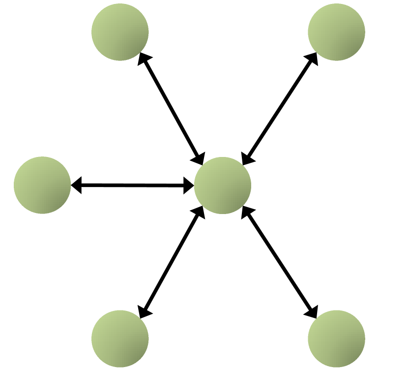
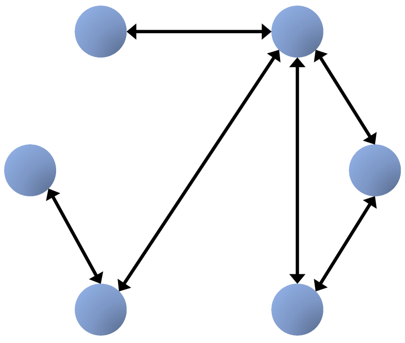
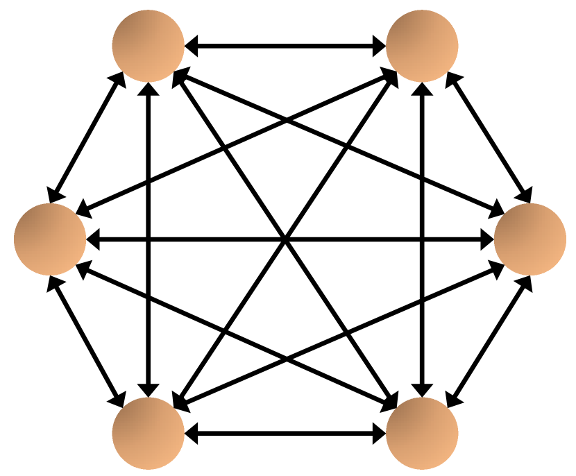
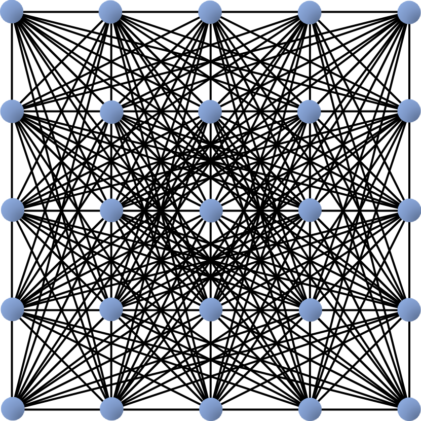
Figure 1: Different network topologies for distributed learning: (a) a non-cooperative topology where agents do not interact with one another, (b) a fully-connected topology where every agent is connected to every other agent in the network, (c) a centralized topology that is equivalent in performance to the fully-connected topology but requires less communication overhead, and (d) a sparsely connected network topology in which each user is connected to a subset of the users in the network.

There are various approaches for optimizing (4). We concentrate on fully-distributed strategies that operate over sparsely-connected networks. The concept of a fully distributed strategy is used here to mean the following:

  • (i)

    There is no central node that is coordinating the communication and computation during the learning process.

  • (ii)

    A node does not need to be connected to all other nodes. Indeed, as long as the network is connected (and it can be sparsely connected), the algorithm is able to approach the solution to the global learning problem.

  • (iii)

    Only one-hop communication is allowed during the learning process. That is, we do not allow the routing of a data packet over the network. Instead, each agent/node is only allowed to be directly communicating with its intermediate neighbors.

Figure 1 illustrates the types of topologies examined in this manuscript. It is important to notice that the centralized and fully-connected topologies are theoretically equivalent, but practically different as the centralized topology greatly reduces the amount of information that is communicated throughout the network. The centralized topology, however, is not robust to node failure since the entire solution breaks down if the central node fails. Throughout the remainder of the manuscript, we will refer to the centralized and fully-connected approaches interchangeably since they have identical excess-risk performance.

II-A Non-Cooperative Strategy

First, we examine the non-cooperative strategy for optimizing (4), which is for each node k𝑘k to run independently a stochastic gradient algorithm of the following form for i1𝑖1i\geq 1 [31, 32, 33, 34]:

𝒘k,i=𝒘k,i1μ(i)wQ(𝒘k,i1,𝒙k,i)[no cooperation]subscript𝒘𝑘𝑖subscript𝒘𝑘𝑖1𝜇𝑖subscript𝑤𝑄subscript𝒘𝑘𝑖1subscript𝒙𝑘𝑖[no cooperation]\displaystyle{\bm{w}}_{k,i}={\bm{w}}_{k,i-1}\!-\!\mu(i)\nabla_{\!w}Q(\!{\bm{w}}_{k,i-1},\!{\bm{x}}_{k,i}\!)\quad\quad\textrm{[no cooperation]} (6)

where wQ()subscript𝑤𝑄\nabla_{w}Q(\cdot) denotes the gradient vector of the loss function, and μ(i)0𝜇𝑖0\mu(i)\geq 0 is a step-size sequence. The gradient vector employed in (6) is an approximation for the actual gradient vector, wJk()subscript𝑤subscript𝐽𝑘\nabla_{w}J_{k}(\cdot), of the risk function. The difference between the true gradient vector and its approximation used in (6) is called gradient noise. Due to the presence of the gradient noise, the estimate 𝒘k,isubscript𝒘𝑘𝑖{\bm{w}}_{k,i} generated by (6) becomes a random quantity; we use boldface letters to refer to random variables throughout our manuscript, which is already reflected in our notation in (6).

It is shown in [31, 35] that for strongly-convex risk functions Jk(w)subscript𝐽𝑘𝑤J_{k}(w), the non-cooperative scheme (6) achieves an asymptotic convergence rate in the order of O(1/i)𝑂1𝑖O(1/i) under some conditions on the gradient noise and the step-size sequence μ(i)𝜇𝑖\mu(i), where the notation f(n)=O(g(n))𝑓𝑛𝑂𝑔𝑛f(n)=O(g(n)) means that the sequence f(n)𝑓𝑛f(n) decays at a rate that is at most the rate of decay of g(n)𝑔𝑛g(n) for sufficiently large n𝑛n—i.e., there exist positive constant c1subscript𝑐1c_{1} and an integer n0subscript𝑛0n_{0} such that f(n)c1g(n)𝑓𝑛subscript𝑐1𝑔𝑛f(n)\leq c_{1}g(n) for all n>n0𝑛subscript𝑛0n>n_{0}. In this way, in order to achieve an excess-risk accuracy on the order of O(ϵ)𝑂italic-ϵO(\epsilon), the non-cooperative algorithm (6) would require O(1/ϵ)𝑂1italic-ϵO(1/\epsilon) samples. It is further shown in [31, 36] that no algorithm can improve upon this rate under the same conditions. This implies that if no cooperation is to take place between the nodes, then the best asymptotic rate each learner would hope to achieve is on the order of O(1/i)𝑂1𝑖O(1/i).

II-B Centralized Strategy

Now, in place of the non-cooperative strategy, let us assume that the N𝑁N nodes transmit their samples to a central processor, which executes the following algorithm:

𝒘i=𝒘i1μ(i)Nk=1NwQ(𝒘i1,𝒙k,i)[unweighted cent.]subscript𝒘𝑖subscript𝒘𝑖1𝜇𝑖𝑁superscriptsubscript𝑘1𝑁subscript𝑤𝑄subscript𝒘𝑖1subscript𝒙𝑘𝑖[unweighted cent.]\displaystyle{\bm{w}}_{i}={\bm{w}}_{i-1}\!-\!\frac{\mu(i)}{N}\!\sum_{k=1}^{N}\nabla_{w}Q({\bm{w}}_{i-1},{\bm{x}}_{k,i})\quad\!\textrm{[unweighted\ cent.]} (7)

It can be shown that this implementation will have an asymptotic convergence rate in the order of O(1/Ni)𝑂1𝑁𝑖O(1/Ni) for step-size sequences of the form μ(i)=μ/i𝜇𝑖𝜇𝑖\mu(i)=\mu/i (see Corollary 2). In other words, the centralized implementation (7) provides an Nlimit-from𝑁N-fold increase in convergence rate relative to the non-cooperative solution (6). One of the questions we wish to answer in this work is whether it is possible to derive a fully distributed algorithm that allows every node in the network to converge (in the mean-square-error sense) at the same rate as the centralized solution, i.e., O(1/Ni)𝑂1𝑁𝑖O(1/Ni), with only communication between neighboring nodes and for general ad-hoc networks. We show that this task is indeed possible. We will additionally show that the distributed strategy can outperform the naïve centralized implementation (7) when the gradient noise profile across the agents is non-uniform, but that it will match the performance of a weighted version of (7), namely, the following weighted centralized strategy:

𝒘i=𝒘i1μ(i)k=1NπkwQ(𝒘i1,𝒙k,i)[weighted cent.]subscript𝒘𝑖subscript𝒘𝑖1𝜇𝑖superscriptsubscript𝑘1𝑁subscript𝜋𝑘subscript𝑤𝑄subscript𝒘𝑖1subscript𝒙𝑘𝑖[weighted cent.]\displaystyle{\bm{w}}_{i}={\bm{w}}_{i-1}\!-\!\mu(i)\!\sum_{k=1}^{N}\pi_{k}\nabla_{w}Q({\bm{w}}_{i-1},{\bm{x}}_{k,i})\quad\!\textrm{[weighted\ cent.]} (8)

where the {πk}subscript𝜋𝑘\{\pi_{k}\} are convex combination weights that satisfy:

πk>0,k=1Nπk=1formulae-sequencesubscript𝜋𝑘0superscriptsubscript𝑘1𝑁subscript𝜋𝑘1\displaystyle\pi_{k}>0,\quad\quad\sum_{k=1}^{N}\pi_{k}=1 (9)

and are meant to discount gradients with higher noise power compared to others. We next describe two popular fully-distributed strategies.

II-C Diffusion Strategy

Following the approach of [14, 32, 34], the diffusion strategy for evaluating distributed estimates 𝒘k,isubscript𝒘𝑘𝑖{\bm{w}}_{k,i} for wosuperscript𝑤𝑜w^{o} in (4) takes the following form:

𝝍k,isubscript𝝍𝑘𝑖\displaystyle\bm{\psi}_{k,i}\! =𝒘k,i1μ(i)wQ(𝒘k,i1,𝒙k,i)absentsubscript𝒘𝑘𝑖1𝜇𝑖subscript𝑤𝑄subscript𝒘𝑘𝑖1subscript𝒙𝑘𝑖\displaystyle=\!{\bm{w}}_{k,i-1}\!-\!\mu(i)\nabla_{w}Q({\bm{w}}_{k,i-1},{\bm{x}}_{k,i}) [adaptation] (10)
𝒘k,isubscript𝒘𝑘𝑖\displaystyle{\bm{w}}_{k,i}\! ==1Nak𝝍,iabsentsuperscriptsubscript1𝑁subscript𝑎𝑘subscript𝝍𝑖\displaystyle=\!\sum_{\ell=1}^{N}a_{\ell k}\bm{\psi}_{\ell,i} [aggregation] (11)

where 𝒙k,isubscript𝒙𝑘𝑖{\bm{x}}_{k,i} denotes the current data sample available at node k𝑘k. Each node k𝑘k begins with an estimate 𝒘k,0subscript𝒘𝑘0{\bm{w}}_{k,0} and employs a diminishing positive step-size sequence μ(i)𝜇𝑖\mu(i). The non-negative coefficients {ak}subscript𝑎𝑘\{a_{\ell k}\}, which form a left-stochastic N×N𝑁𝑁N\times N combination matrix A=[ak]𝐴delimited-[]subscript𝑎𝑘A=[a_{\ell k}], are used to scale information arriving at node k𝑘k from its neighbors. These coefficients are chosen to satisfy:

=1𝑁ak=1,ak=0 if nodes (,k) are not connectedformulae-sequence1𝑁subscript𝑎𝑘1subscript𝑎𝑘0 if nodes 𝑘 are not connected\displaystyle\underset{\ell=1}{\overset{N}{\sum}}a_{\ell k}\!=\!1,\ a_{\ell k}=0\textrm{ if nodes }(\ell,\!k)\textrm{ are not connected} (12)

We emphasize that we are only requiring A𝐴A to be left-stochastic, meaning that only each of its columns should add up to one rather than each of its columns and rows. The neighborhood 𝒩ksubscript𝒩𝑘\mathcal{N}_{k} for each node k𝑘k is defined as the set of nodes {}\{\ell\} for which ak0subscript𝑎𝑘0a_{\ell k}\neq 0. The neighborhood 𝒩ksubscript𝒩𝑘\mathcal{N}_{k} is typically known to agent k𝑘k. The main difference between the above algorithm and the original adapt-then-combine (ATC) diffusion strategy studied in [14, 34, 32] is that we are employing a diminishing step-size sequence μ(i)𝜇𝑖\mu(i) as opposed to a constant step-size. Constant step-sizes have the distinct advantage that they allow nodes to continue adapting their estimates in response to drifts in the underlying data distribution [37]. In this work, we are interested in examining the generalization ability of distributed learners asymptotically when the underlying distribution, 𝒳ksubscript𝒳𝑘{\cal X}_{k}, remains stationary, in which case the use of decaying step-sizes sequences is justified. If the statistical distribution of the data were subject to drifts, then constant step-sizes become a necessity, and this scenario is already studied in some detail in [14, 15, 34, 32].

II-D Consensus Strategy

In addition to (10)–(11), we shall examine the following consensus-based implementation [4, 17, 18, 33] for solving the same problem (4):

𝒘k,i==1Nak𝒘,i1μ(i)wQ(𝒘k,i1,𝒙k,i)[consensus]subscript𝒘𝑘𝑖superscriptsubscript1𝑁subscript𝑎𝑘subscript𝒘𝑖1𝜇𝑖subscript𝑤𝑄subscript𝒘𝑘𝑖1subscript𝒙𝑘𝑖[consensus]{\bm{w}}_{k,i}=\sum_{\ell=1}^{N}\!a_{\ell k}{\bm{w}}_{\ell,i-1}\!-\!\mu(i)\nabla_{w}Q({\bm{w}}_{k,i-1},{\bm{x}}_{k,i})\quad\textrm{[consensus]} (13)

The diffusion and consensus strategies (10)-(13) have exactly the same computational complexity, except that the computations are performed in a different order. We will see in Sec. IV-D that this difference enhances the performance of diffusion over consensus. Moreover, in the constant step-size case, the difference in the order in which the operations are performed causes an anomaly in the behavior of consensus solutions in that they can become unstable even when all individual nodes are able to solve the inference task in a stable manner; see [20, 34, 32]. Furthermore, consensus strategies of the form (13) are usually limited to employing a doubly-stochastic combination matrix A𝐴A. The analysis in the sequel will show that left-stochastic matrices actually lead to improved excess-risk performance (see Eqs. (61)–(63)) while convergence of the distributed implementation continues to be guaranteed (see Theorem 1).

III Main Assumptions

Before proceeding with the analysis, we list in this section the main assumptions that are needed to facilitate the exposition. The conditions listed below are common in the broad stochastic optimization literature — see the explanations in [31, 33, 34, 32]. The first condition assumes that the Jk(w)subscript𝐽𝑘𝑤J_{k}(w) are strongly-convex, with a common minimizer wosuperscript𝑤𝑜w^{o} for k=1,,N𝑘1𝑁k=1,\ldots,N. This condition ensures that the optimization problem (4) is well-conditioned.

Assumption 1 (Properties of risk functions)

Each risk function Jk(w)subscript𝐽𝑘𝑤J_{k}(w) is twice continuously-differentiable and its Hessian matrix is uniformly bounded from below and from above, namely,

0<λ¯Iw2Jk(w)λ¯I<0¯𝜆𝐼subscriptsuperscript2𝑤subscript𝐽𝑘𝑤¯𝜆𝐼0<\underline{\lambda}I\leq\nabla^{2}_{w}J_{k}(w)\leq\overline{\lambda}{I}<\infty (14)

Furthermore, the risks at the various agents are minimized at the same location:

wo=argmin𝑤Jk(w),k=1,,Nformulae-sequencesuperscript𝑤𝑜𝑤subscript𝐽𝑘𝑤𝑘1𝑁\displaystyle w^{o}=\underset{w}{\arg\min}\ J_{k}(w),\quad\quad k=1,\ldots,N (15)

and the Hessian matrices are locally Lipschitz continuous at wosuperscript𝑤𝑜w^{o}, i.e., for all wow<εnormsuperscript𝑤𝑜𝑤𝜀\|w^{o}-w\|<\varepsilon, there exists some τk0subscript𝜏𝑘0\tau_{k}\geq 0 such that:

w2Jk(wo)w2Jk(w)τkwownormsubscriptsuperscript2𝑤subscript𝐽𝑘superscript𝑤𝑜subscriptsuperscript2𝑤subscript𝐽𝑘𝑤subscript𝜏𝑘normsuperscript𝑤𝑜𝑤\displaystyle\|\nabla^{2}_{w}J_{k}(w^{o})-\nabla^{2}_{w}J_{k}(w)\|\leq\tau_{k}\cdot\|w^{o}-w\| (16)

We denote the value of the Hessian matrices at w=wo𝑤superscript𝑤𝑜w=w^{o} (assumed uniform across the agents) by

Hw2Jk(wo),k=1,,Nformulae-sequence𝐻superscriptsubscript𝑤2subscript𝐽𝑘superscript𝑤𝑜𝑘1𝑁\displaystyle H\triangleq\nabla_{w}^{2}J_{k}(w^{o}),\quad\quad k=1,\ldots,N (17)

where H>0𝐻0H>0. We let λmin>0subscript𝜆0\lambda_{\min}>0 denote the smallest eigenvalue of H𝐻H. \blacksquare

In fact, conditions (14) and the locally Lipschitz condition (16) jointly imply (16) globally (see Lemma E.8 in [32]); i.e., for all wM×1𝑤superscript𝑀1w\in\mathbb{R}^{M\times 1}, we have that there exists some τksubscript𝜏𝑘\tau_{k} such that:

w2Jk(wo)w2Jk(w)τkwownormsubscriptsuperscript2𝑤subscript𝐽𝑘superscript𝑤𝑜subscriptsuperscript2𝑤subscript𝐽𝑘𝑤subscript𝜏𝑘normsuperscript𝑤𝑜𝑤\displaystyle\|\nabla^{2}_{w}J_{k}(w^{o})-\nabla^{2}_{w}J_{k}(w)\|\leq\tau_{k}\cdot\|w^{o}-w\| (18)

Observe that

λminλ¯subscript𝜆¯𝜆\displaystyle\lambda_{\min}\geq\underline{\lambda} (19)

One useful implication that follows from Assumption 1 is the following. Consider the expected excess-risk (5) at node k𝑘k. Using the following sequence of inequalities, we can bound the excess-risk by a square weighted norm:

ERk(i)subscriptER𝑘𝑖\displaystyle\textrm{ER}_{k}(i) 𝔼𝒘{Jk(𝒘k,i1)Jk(wo)}absentsubscript𝔼𝒘subscript𝐽𝑘subscript𝒘𝑘𝑖1subscript𝐽𝑘superscript𝑤𝑜\displaystyle\triangleq\mathbb{E}_{\bm{w}}\{J_{k}({\bm{w}}_{k,i-1})-J_{k}(w^{o})\}
=(a)𝔼𝒘𝒘~k,i1𝑺k,i2superscriptaabsentsubscript𝔼𝒘superscriptsubscriptnormsubscript~𝒘𝑘𝑖1subscript𝑺𝑘𝑖2\displaystyle\stackrel{{\scriptstyle\mathrm{(a)}}}{{=}}\mathbb{E}_{\bm{w}}\|\widetilde{{\bm{w}}}_{k,i-1}\|_{{\bm{S}}_{k,i}}^{2} (20a)
(b)λ¯2𝔼𝒘𝒘~k,i12superscriptbabsent¯𝜆2subscript𝔼𝒘superscriptnormsubscript~𝒘𝑘𝑖12\displaystyle\stackrel{{\scriptstyle\mathrm{(b)}}}{{\leq}}\frac{\overline{\lambda}}{2}\cdot\mathbb{E}_{\bm{w}}\|\widetilde{{\bm{w}}}_{k,i-1}\|^{2} (20b)

where 𝒘~k,iwo𝒘k,isubscript~𝒘𝑘𝑖superscript𝑤𝑜subscript𝒘𝑘𝑖\widetilde{{\bm{w}}}_{k,i}\triangleq w^{o}-{\bm{w}}_{k,i}, 𝔼𝒘{}subscript𝔼𝒘{\mathbb{E}}_{\bm{w}}\{\cdot\} denotes expectation over the distribution of 𝒘𝒘{\bm{w}}, and the weighting matrix 𝑺k,isubscript𝑺𝑘𝑖\bm{S}_{k,i} is defined as

𝑺k,i[01t01w2Jk(wost𝒘~k,i1)𝑑s𝑑t]subscript𝑺𝑘𝑖delimited-[]superscriptsubscript01𝑡superscriptsubscript01superscriptsubscript𝑤2subscript𝐽𝑘superscript𝑤𝑜𝑠𝑡subscript~𝒘𝑘𝑖1differential-d𝑠differential-d𝑡\displaystyle\bm{S}_{k,i}\triangleq\left[\int_{0}^{1}t\int_{0}^{1}\nabla_{w}^{2}J_{k}(w^{o}-s\ t\ \widetilde{{\bm{w}}}_{k,i-1})dsdt\right] (21)

Step (a) is a consequence of applying the following mean-value theorem [31, p. 24] [32] twice for an arbitrary real-valued differentiable function f()𝑓f(\cdot):

f(a+b)=f(a)+(01𝖳f(a+tb)𝑑t)b𝑓𝑎𝑏𝑓𝑎superscriptsubscript01superscript𝖳𝑓𝑎𝑡𝑏differential-d𝑡𝑏f(a+b)=f(a)+\left(\int_{0}^{1}\nabla^{\mathsf{T}}f(a+t\cdot b)\ dt\right)\cdot b (22)

and the fact that wosuperscript𝑤𝑜w^{o} optimizes Jk(w)subscript𝐽𝑘𝑤J_{k}(w) so that wJk(wo)=0subscript𝑤subscript𝐽𝑘superscript𝑤𝑜0\nabla_{w}J_{k}(w^{o})=0. Step (b) is due to (14) and (21).

Expression (20a) shows that the expected excess-risk at node k𝑘k is equal to a weighted mean-square-error with weight matrix (21). This means that one way to compute or bound the expected excess-risk is by evaluating weighted mean-square-error quantities of the form (20a) or (20b). This is the route that we will follow in this manuscript. We will analyze the right-hand side of (20a) in order to draw conclusions regarding the evolution of the expected excess-risk. In particular, once we establish that the distributed algorithm converges in the mean-square-error sense, then inequality (20b) will immediately allow us to conclude that the algorithm also converges in excess-risk. Similarly, we can obtain the asymptotic expression for the excess-risk by leveraging the weighted-mean-square-error analysis developed for constant step-size distributed strategies [14, 15, 32], adjusted for the decaying step-size case. Observe that these conclusions are different than the useful results in [16], which focused on studying convergence in distribution. The mean-square-error results will enable us to expose analytically various interesting differences in the performance of distributed strategies, such as diffusion and consensus.

Our second condition is on the gradient noise process, which is defined, for a generic vector 𝒘𝒘{\bm{w}}, as

𝒗k,i(𝒘)wQ(𝒘,𝒙k,i)wJk(𝒘)subscript𝒗𝑘𝑖𝒘subscript𝑤𝑄𝒘subscript𝒙𝑘𝑖subscript𝑤subscript𝐽𝑘𝒘\displaystyle{\bm{v}}_{k,i}({\bm{w}})\triangleq\nabla_{w}Q({\bm{w}},{\bm{x}}_{k,i})-\nabla_{w}J_{k}({\bm{w}}) (23)

We collect the noises from across the network into a column vector

𝒈i(𝓦)subscript𝒈𝑖𝓦\displaystyle{\bm{g}}_{i}(\bm{{\scriptstyle{\mathcal{W}}}}) col{𝒗1,i(𝒘1),,𝒗N,i(𝒘N)}absentcolsubscript𝒗1𝑖subscript𝒘1subscript𝒗𝑁𝑖subscript𝒘𝑁\displaystyle\triangleq\textrm{col}\{{\bm{v}}_{1,i}({\bm{w}}_{1}),\ldots,{\bm{v}}_{N,i}({\bm{w}}_{N})\} (24)

where we are introducing the vector notation

𝓦𝓦\displaystyle\bm{{\scriptstyle{\mathcal{W}}}} col{𝒘1,,𝒘N}absentcolsubscript𝒘1subscript𝒘𝑁\displaystyle\triangleq\mathrm{col}\{{\bm{w}}_{1},\ldots,{\bm{w}}_{N}\} (25)

for the collection of parameters across the agents. We denote the covariance matrix of the gradient noise vector by

g,i(𝓦)subscript𝑔𝑖𝓦\displaystyle\mathcal{R}_{g,i}(\bm{{\scriptstyle{\mathcal{W}}}}) 𝔼{𝒈i(𝓦)𝒈i𝖳(𝓦)|𝓕i1}absent𝔼conditional-setsubscript𝒈𝑖𝓦superscriptsubscript𝒈𝑖𝖳𝓦subscript𝓕𝑖1\displaystyle\triangleq{\mathbb{E}}\{{\bm{g}}_{i}(\bm{{\scriptstyle{\mathcal{W}}}}){\bm{g}}_{i}^{\mathsf{T}}(\bm{{\scriptstyle{\mathcal{W}}}})|\bm{\mathcal{F}}_{i-1}\} (26)

where the conditioning is in relation to the past history of the estimators, 𝓕i1{𝒘k,j:k=1,,Nandji1}subscript𝓕𝑖1conditional-setsubscript𝒘𝑘𝑗formulae-sequence𝑘1𝑁and𝑗𝑖1\bm{\mathcal{F}}_{i-1}\!\triangleq\!\{{\bm{w}}_{k,j}:k=1,\ldots,N\ \mathrm{and}\ j\leq i-1\}. The following conditions are relaxations of assumptions that are regularly considered in the stochastic approximation literature; they are generally satisfied in important scenarios, such as logistic regression or quadratic loss functions of the form (1)–(2) — see [32].

Assumption 2 (Gradient noise model)

We assume the gradient noise process satisfies:

𝔼{𝒗k,i(𝒘)|𝓕i1}=0𝔼conditional-setsubscript𝒗𝑘𝑖𝒘subscript𝓕𝑖10\displaystyle\mathbb{E}\{{\bm{v}}_{k,i}({\bm{w}})|\bm{\mathcal{F}}_{i-1}\}=0 (27)
𝔼{𝒗k,i(𝒘)4|𝓕i1}α4wo𝒘4+σv44𝔼conditionalsuperscriptnormsubscript𝒗𝑘𝑖𝒘4subscript𝓕𝑖1subscript𝛼4superscriptnormsuperscript𝑤𝑜𝒘4superscriptsubscript𝜎𝑣44\displaystyle\mathbb{E}\{\|{\bm{v}}_{k,i}({\bm{w}})\|^{4}|\bm{\mathcal{F}}_{i-1}\}\leq\alpha_{4}\|w^{o}-{\bm{w}}\|^{4}+\sigma_{v4}^{4} (28)
𝔼{𝒗k,i𝖳(wo)𝒗,i(wo)}=0,kformulae-sequence𝔼superscriptsubscript𝒗𝑘𝑖𝖳superscript𝑤𝑜subscript𝒗𝑖superscript𝑤𝑜0𝑘\displaystyle{\mathbb{E}}\{{\bm{v}}_{k,i}^{\mathsf{T}}(w^{o}){\bm{v}}_{\ell,i}(w^{o})\}=0,\quad k\neq\ell (29)

for some α40subscript𝛼40\alpha_{4}\geq 0, σv440superscriptsubscript𝜎𝑣440\sigma_{v4}^{4}\geq 0, as well as:

g,i(𝒲)g,i(𝟙Nwo)κ𝟙Nwo𝒲γnormsubscript𝑔𝑖𝒲subscript𝑔𝑖tensor-productsubscript1𝑁superscript𝑤𝑜𝜅superscriptnormtensor-productsubscript1𝑁superscript𝑤𝑜𝒲𝛾\displaystyle\|\mathcal{R}_{g,i}({\scriptstyle{\mathcal{W}}})-\mathcal{R}_{g,i}(\mathds{1}_{N}\!\otimes\!w^{o})\|\leq\kappa\|\mathds{1}_{N}\!\otimes\!w^{o}-{\scriptstyle{\mathcal{W}}}\|^{\gamma} (30)
limi𝔼{g,i(𝟙Nwo)}gosubscript𝑖𝔼subscript𝑔𝑖tensor-productsubscript1𝑁superscript𝑤𝑜superscriptsubscript𝑔𝑜\displaystyle\lim_{i\rightarrow\infty}{\mathbb{E}}\{\mathcal{R}_{g,i}(\mathds{1}_{N}\otimes w^{o})\}\triangleq\mathcal{R}_{g}^{o} (31)

for some κ0𝜅0\kappa\geq 0, 0<γ40𝛾40<\gamma\leq 4, and where

𝒲𝒲\displaystyle{\scriptstyle{\mathcal{W}}} col{w1,,wN}absentcolsubscript𝑤1subscript𝑤𝑁\displaystyle\triangleq\mathrm{col}\{w_{1},\ldots,w_{N}\} (32)

and (30) is assumed to hold for 𝟙Nwo𝒲ϵnormtensor-productsubscript1𝑁superscript𝑤𝑜𝒲italic-ϵ\|\mathds{1}_{N}\!\otimes\!w^{o}-{\scriptstyle{\mathcal{W}}}\|\leq\epsilon, for some small ϵ>0italic-ϵ0\epsilon>0. \blacksquare

Observe that Assumption 2 implies that:

𝔼{𝒗k,i(𝒘)2|𝓕i1}𝔼conditionalsuperscriptnormsubscript𝒗𝑘𝑖𝒘2subscript𝓕𝑖1\displaystyle\mathbb{E}\{\|{\bm{v}}_{k,i}({\bm{w}})\|^{2}|\bm{\mathcal{F}}_{i-1}\} α2wo𝒘2+σv22absentsubscript𝛼2superscriptnormsuperscript𝑤𝑜𝒘2superscriptsubscript𝜎𝑣22\displaystyle\leq\alpha_{2}\cdot\|w^{o}\!-\!{\bm{w}}\|^{2}\!+\!\sigma_{v2}^{2} (33)

for some α2,σv220subscript𝛼2superscriptsubscript𝜎𝑣220\alpha_{2},\sigma_{v2}^{2}\geq 0 and 𝒘𝓕i1𝒘subscript𝓕𝑖1{\bm{w}}\in\bm{\mathcal{F}}_{i-1}. In addition, the local Lipschitz condition (30) of order γ𝛾\gamma [38, p. 53] (sometimes referred to as the Hölder condition of order γ𝛾\gamma [39, p. 110]) implies, under Assumption 1, that the following global condition also holds [32, 15]:

g,i(𝒲)g,i(𝟙Nwo)normsubscript𝑔𝑖𝒲subscript𝑔𝑖tensor-productsubscript1𝑁superscript𝑤𝑜\displaystyle\|\mathcal{R}_{g,i}({\scriptstyle{\mathcal{W}}})-\mathcal{R}_{g,i}(\mathds{1}_{N}\!\otimes\!w^{o})\| κ1𝟙Nwo𝒲2+absentlimit-fromsubscript𝜅1superscriptnormtensor-productsubscript1𝑁superscript𝑤𝑜𝒲2\displaystyle\leq\kappa_{1}\|\mathds{1}_{N}\!\otimes\!w^{o}-{\scriptstyle{\mathcal{W}}}\|^{2}+
κ𝟙Nwo𝒲γ𝜅superscriptnormtensor-productsubscript1𝑁superscript𝑤𝑜𝒲𝛾\displaystyle\quad\ \kappa\|\mathds{1}_{N}\!\otimes\!w^{o}-{\scriptstyle{\mathcal{W}}}\|^{\gamma} (34)

for some constant κ10subscript𝜅10\kappa_{1}\geq 0 that depends on ϵitalic-ϵ\epsilon and where κ𝜅\kappa is from (30). Furthermore, due to (29), we have that the matrix gosuperscriptsubscript𝑔𝑜\mathcal{R}_{g}^{o} is block-diagonal:

gosuperscriptsubscript𝑔𝑜\displaystyle\mathcal{R}_{g}^{o} blockdiag{Rv,1o,,Rv,No}absentblockdiagsuperscriptsubscript𝑅𝑣1𝑜superscriptsubscript𝑅𝑣𝑁𝑜\displaystyle\triangleq\textrm{blockdiag}\{R_{v,1}^{o},\ldots,R_{v,N}^{o}\} (35)
Rv,kosuperscriptsubscript𝑅𝑣𝑘𝑜\displaystyle R_{v,k}^{o} limi𝔼{𝒗k,i(wo)𝒗k,i𝖳(wo)}absentsubscript𝑖𝔼subscript𝒗𝑘𝑖superscript𝑤𝑜superscriptsubscript𝒗𝑘𝑖𝖳superscript𝑤𝑜\displaystyle\triangleq\lim_{i\rightarrow\infty}{\mathbb{E}}\{{\bm{v}}_{k,i}(w^{o}){\bm{v}}_{k,i}^{\mathsf{T}}(w^{o})\} (36)

Since nodes sample the data in an independent fashion, it is reasonable to expect the gradient noise to be uncorrelated across all nodes, as required by (29).

Our third condition relates to the structure of the network topology. We will assume that the network is strongly-connected, which means that (a) there exists at least one nontrivial self-loop, akk>0subscript𝑎𝑘𝑘0a_{kk}>0 for some k𝑘k, and (b) for any two agents k𝑘k and \ell, there exists a path with nonzero weights {ak,m1,am1,m2,,amr,}subscript𝑎𝑘subscript𝑚1subscript𝑎subscript𝑚1subscript𝑚2subscript𝑎subscript𝑚𝑟\{a_{k,m_{1}},a_{m_{1},m_{2}},\ldots,a_{m_{r},\ell}\} from k𝑘k to \ell, either directly if they are neighbors or through other agents. It is well-known that the combination matrix A𝐴A for such networks is primitive [40, p. 516]. That is, all entries of A𝐴A are non-negative and there exists some positive integer no>0subscript𝑛𝑜0n_{o}>0 such that all entries of Anosuperscript𝐴subscript𝑛𝑜A^{n_{o}} are strictly positive. One important property of primitive matrices follows from the Perron-Frobenius theorem [40, p. 534]; A𝐴A will have a single eigenvalue at one, while all other eigenvalues of A𝐴A will lie strictly inside the unit circle. Moreover, if we let p𝑝p denote the right-eigenvector associated with the eigenvalue at one, and normalize its entries to add up to one, i.e.,

Ap=p,    1N𝖳p=1formulae-sequence𝐴𝑝𝑝superscriptsubscript1𝑁𝖳𝑝1Ap=p,\;\;\;\;\mathds{1}_{N}^{\mathsf{T}}p=1 (37)

then all entries of p𝑝p will be strictly positive. We shall refer to p𝑝p as the Perron eigenvector of A𝐴A. We formalize this assumption in the following:

Assumption 3 (Network Topology)

The network is strongly-connected so that the combination matrix A𝐴A is primitive with 𝟙𝖳p=1superscript1𝖳𝑝1\mathds{1}^{\mathsf{T}}p=1 and p0succeeds𝑝0p\succ 0, where p𝑝p denotes the the Perron eigenvector of A𝐴A. \blacksquare

IV Main Results

In this section, we list the main results and defer the detailed proofs to the appendices.

IV-A Convergence Properties

Our first result provides conditions on the step-size sequence under which the diffusion strategy converges both in the mean-square-error (MSE) sense and also almost surely. The difference between the two sets of conditions that appear below is that in one case the step-size sequence is additionally required to be square-summable.

Theorem 1 (Convergence rates)

Let Assumptions 1-3 hold and let the step-size sequence satisfy

μ(i)>0,i=1μ(i)=,limiμ(i)=0.formulae-sequence𝜇𝑖0formulae-sequencesuperscriptsubscript𝑖1𝜇𝑖subscript𝑖𝜇𝑖0\displaystyle\mu(i)>0,\quad\sum_{i=1}^{\infty}\mu(i)=\infty,\quad\lim_{i\rightarrow\infty}\mu(i)=0. (38)

Then, 𝐰k,isubscript𝐰𝑘𝑖{\bm{w}}_{k,i} generated by (10)–(11) converges in the MSE sense to wosuperscript𝑤𝑜w^{o}, i.e.,

limi𝔼wo𝒘k,i2=0.subscript𝑖𝔼superscriptnormsuperscript𝑤𝑜subscript𝒘𝑘𝑖20\displaystyle\lim_{i\rightarrow\infty}{\mathbb{E}}\|w^{o}-{\bm{w}}_{k,i}\|^{2}=0. (39)

If the step-size sequence satisfies the additional square-summability condition:

i=1μ2(i)<,superscriptsubscript𝑖1superscript𝜇2𝑖\displaystyle\sum_{i=1}^{\infty}\mu^{2}(i)<\infty, (40)

then 𝐰k,isubscript𝐰𝑘𝑖{\bm{w}}_{k,i} converges to wosuperscript𝑤𝑜w^{o} almost surely (i.e., with probability one) for all k=1,,N𝑘1𝑁k=1,\ldots,N. Furthermore, when the step-size sequence is of the form μ(i)=μ/i𝜇𝑖𝜇𝑖\mu(i)=\mu/i with μ𝜇\mu satisfying 2λ¯μ>12¯𝜆𝜇12\underline{\lambda}\mu>1, then the second and fourth-order moments of the error vector converge at the rates of O(1/i)𝑂1𝑖O(1/i) and O(1/i2)𝑂1superscript𝑖2O(1/i^{2}), respectively:

lim supi𝔼𝒘~k,i2i1subscriptlimit-supremum𝑖𝔼superscriptnormsubscript~𝒘𝑘𝑖2superscript𝑖1\displaystyle\limsup_{i\rightarrow\infty}\frac{{\mathbb{E}}\|\widetilde{{\bm{w}}}_{k,i}\|^{2}}{i^{-1}} σv22μ22λ¯μ1absentsuperscriptsubscript𝜎𝑣22superscript𝜇22¯𝜆𝜇1\displaystyle\leq\frac{\sigma_{v2}^{2}\mu^{2}}{2\underline{\lambda}\mu-1} (41)
lim supi𝔼𝒘~k,i4i2subscriptlimit-supremum𝑖𝔼superscriptnormsubscript~𝒘𝑘𝑖4superscript𝑖2\displaystyle\limsup_{i\rightarrow\infty}\frac{{\mathbb{E}}\|\widetilde{{\bm{w}}}_{k,i}\|^{4}}{i^{-2}} constantabsentconstant\displaystyle\leq\textrm{constant} (42)

where σv22superscriptsubscript𝜎𝑣22\sigma_{v2}^{2} was introduced in (33).

Proof:

See Appendix A. \blacksquare

Observe that (41) implies that each node converges in the mean-square-error sense at the rate 1/i1𝑖1/i. Combining this result with (20b), we conclude that each node also converges in excess-risk at this rate:

lim supiERk(i)i1subscriptlimit-supremum𝑖subscriptER𝑘𝑖superscript𝑖1\displaystyle\limsup_{i\rightarrow\infty}\frac{\mathrm{ER}_{k}(i)}{i^{-1}} μ2λ¯μ2λ¯μ1σv22absent𝜇2¯𝜆𝜇2¯𝜆𝜇1superscriptsubscript𝜎𝑣22\displaystyle\leq\frac{\mu}{2}\cdot\frac{\bar{\lambda}\mu}{2\underline{\lambda}\mu-1}\cdot\sigma_{v2}^{2} (43)

when 2λ¯μ>12¯𝜆𝜇12\underline{\lambda}\mu>1.

Note that this conclusion does not yet reveal the benefit of cooperation (for example, it does not show how the convergence rate depends on N𝑁N). In the next section, we will derive closed-form asymptotic expressions for the mean-square-error and excess-risk, and from these expressions we will be able to highlight the benefit of network cooperation.

IV-B Evolution of Excess-Risk Measure

We continue to assume that the step-size sequence is selected as μ(i)=μ/i𝜇𝑖𝜇𝑖\mu(i)=\mu/i for some μ>0𝜇0\mu>0. This sequence satisfies conditions (38) and (40). Observe that in order to evaluate the excess-risk at node k𝑘k, we must evaluate (20a). To do so, we first form the following network-wide error quantity:

𝓦~isubscript~𝓦𝑖\displaystyle\widetilde{\bm{{\scriptstyle{\mathcal{W}}}}}_{i} col{𝒘~1,i,,𝒘~N,i}absentcolsubscript~𝒘1𝑖subscript~𝒘𝑁𝑖\displaystyle\triangleq\mathrm{col}\{\widetilde{{\bm{w}}}_{1,i},\ldots,\widetilde{{\bm{w}}}_{N,i}\} (44)

and let Ekksubscript𝐸𝑘𝑘E_{kk} denote the N×N𝑁𝑁N\times N matrix with a single entry equal to one at the (k,k)limit-from𝑘𝑘(k,k)-th location and all other entries equal to zero. Then, using (20a), we can write:

ERk(i)𝔼𝓦~i1Ekk𝑺k,i2subscriptER𝑘𝑖𝔼subscriptsuperscriptnormsubscript~𝓦𝑖12tensor-productsubscript𝐸𝑘𝑘subscript𝑺𝑘𝑖\displaystyle\textrm{ER}_{k}(i)\triangleq{\mathbb{E}}\|\widetilde{\bm{{\scriptstyle{\mathcal{W}}}}}_{i-1}\|^{2}_{E_{kk}\otimes\bm{S}_{k,i}} (45)

In order to facilitate the analysis, we introduce the eigenvalue decomposition of matrix H𝐻H:

H=ΦΛΦ𝖳𝐻ΦΛsuperscriptΦ𝖳\displaystyle H=\Phi\Lambda\Phi^{\mathsf{T}} (46)

where ΦΦ\Phi is an orthogonal matrix and ΛΛ\Lambda is diagonal with positive entries λ1,λ2,,λMsubscript𝜆1subscript𝜆2subscript𝜆𝑀\lambda_{1},\lambda_{2},\ldots,\lambda_{M}. Moreover, since the matrix A𝐴A is left-stochastic and primitive (by Assumption 3), we can express its Jordan decomposition in the form:

A=p𝟙𝖳+YDN1R𝖳𝐴𝑝superscript1𝖳𝑌subscript𝐷𝑁1superscript𝑅𝖳\displaystyle A=p\mathds{1}^{\mathsf{T}}+YD_{N-1}R^{\mathsf{T}} (47)

where R,YN×N1𝑅𝑌superscript𝑁𝑁1R,Y\in\mathbb{R}^{N\times N-1} represent the remaining left and right eigenvectors while DN1subscript𝐷𝑁1D_{N-1} represents the Jordan structure associated with the eigenvalues inside the unit disc.

Theorem 2 (Asymptotic Convergence of ERk(i)subscriptER𝑘𝑖\mathrm{ER}_{k}(i))

Let Assumptions 1-3 hold and let λminsubscript𝜆\lambda_{\min} denote the smallest eigenvalue of the matrix H𝐻H:

λminmin{λ1,,λM}subscript𝜆subscript𝜆1subscript𝜆𝑀\displaystyle\lambda_{\min}\triangleq\min\{\lambda_{1},\ldots,\lambda_{M}\} (48)

Then, when 2λminμ>12subscript𝜆𝜇12\lambda_{\min}\mu>1, it holds asymptotically that

ERk(i)subscriptER𝑘𝑖\displaystyle\mathrm{ER}_{k}(i) μ2im=1Mλmμ2λmμ1p𝖳Rv,mpsimilar-toabsent𝜇2𝑖superscriptsubscript𝑚1𝑀subscript𝜆𝑚𝜇2subscript𝜆𝑚𝜇1superscript𝑝𝖳subscript𝑅𝑣𝑚𝑝\displaystyle\sim\frac{\mu}{2i}\cdot\sum_{m=1}^{M}\frac{\lambda_{m}\mu}{2\lambda_{m}\mu-1}\cdot p^{\mathsf{T}}R_{v,m}p (49)
=μ2im=1Mλmμ2λmμ1=1Np2(Φ𝖳Rv,oΦ)mmabsent𝜇2𝑖superscriptsubscript𝑚1𝑀subscript𝜆𝑚𝜇2subscript𝜆𝑚𝜇1superscriptsubscript1𝑁superscriptsubscript𝑝2subscriptsuperscriptΦ𝖳superscriptsubscript𝑅𝑣𝑜Φ𝑚𝑚\displaystyle=\frac{\mu}{2i}\cdot\sum_{m=1}^{M}\frac{\lambda_{m}\mu}{2\lambda_{m}\mu-1}\sum_{\ell=1}^{N}p_{\ell}^{2}(\Phi^{{\mathsf{T}}}R_{v,\ell}^{o}\Phi)_{mm} (50)

where the notation f(i)g(i)similar-to𝑓𝑖𝑔𝑖f(i)\!\sim\!g(i) implies that limif(i)/g(i)=1subscript𝑖𝑓𝑖𝑔𝑖1\displaystyle{\lim_{i\rightarrow\infty}}f(i)/g(i)\!=\!1. Moreover, λmsubscript𝜆𝑚\lambda_{m} is the m𝑚m-th eigenvalue of H𝐻H and the N×N𝑁𝑁N\times N matrix Rv,msubscript𝑅𝑣𝑚R_{v,m} is defined as:

Rv,m[(Φ𝖳Rv,1oΦ)mm(Φ𝖳Rv,NoΦ)mm]subscript𝑅𝑣𝑚delimited-[]subscriptsuperscriptΦ𝖳superscriptsubscript𝑅𝑣1𝑜Φ𝑚𝑚missing-subexpressionmissing-subexpressionmissing-subexpressionmissing-subexpressionmissing-subexpressionmissing-subexpressionsubscriptsuperscriptΦ𝖳superscriptsubscript𝑅𝑣𝑁𝑜Φ𝑚𝑚\displaystyle R_{v,m}\triangleq\left[\begin{array}[]{ccc}(\Phi^{\mathsf{T}}R_{v,1}^{o}\Phi)_{mm}&&\\ &\ddots&\\ &&(\Phi^{\mathsf{T}}R_{v,N}^{o}\Phi)_{mm}\end{array}\right] (54)

where the notation (X)mmsubscript𝑋𝑚𝑚(X)_{mm} denotes the m𝑚m-th diagonal element of the matrix X𝑋X.

Proof:

See Appendix B. \blacksquare

Theorem 2 establishes a closed-form expression for the asymptotic excess-risk of the diffusion algorithm. We observe that the slowest rate at which the asymptotic term converges depends on the smallest eigenvalue of H𝐻H, which is λminsubscript𝜆\lambda_{\min}, and the constant μ𝜇\mu. Interestingly, the only dependence on the topology of the network asymptotically is encoded in the Perron vector p𝑝p of the combination matrix A𝐴A—i.e., most of the eigen-structure of the topology matrices becomes irrelevant asymptotically and only influences the convergence rate in the transient regime. We will see further ahead that the Perron vector p𝑝p can be optimized to minimize the excess-risk in the asymptotic regime. It is natural that the transient stage should depend on the network geometry because the networked agents are propagating their information over the entire network. The speed of information propagation over a sparsely connected network is determined by the second largest eigenvalue of the combination matrix [14], which is influenced by the degree of network connectivity. Our results show, however, that there is an asymptotic regime where the performance of the diffusion strategy can be made invariant to the specific network topology since the Perron vector p𝑝p can be designed for general connected networks, as we will see further ahead in (63). Finally, we observe that all agents participating in the network will achieve the same asymptotic performance given by the right-hand-side of (49) as this asymptotic expression for the excess-risk does not depend on any particular node index k𝑘k but only on the network-wide quantity p𝖳Rv,mpsuperscript𝑝𝖳subscript𝑅𝑣𝑚𝑝p^{\mathsf{T}}R_{v,m}p.

When λminsubscript𝜆\lambda_{\min} is not known, and thus it is not clear how to choose μ𝜇\mu to satisfy 2λminμ>12subscript𝜆𝜇12\lambda_{\min}\mu>1, it is common to choose a large μ𝜇\mu that forces 2λminμ1much-greater-than2subscript𝜆𝜇12\lambda_{\min}\mu\gg 1. In this case, we obtain from (50) that

ERk(i)subscriptER𝑘𝑖\displaystyle\mathrm{ER}_{k}(i) μ4i=1Np2𝖳𝗋(Rv,o),[2λminμ1]absent𝜇4𝑖superscriptsubscript1𝑁superscriptsubscript𝑝2𝖳𝗋superscriptsubscript𝑅𝑣𝑜delimited-[]much-greater-than2subscript𝜆𝜇1\displaystyle\approx\frac{\mu}{4i}\cdot\sum_{\ell=1}^{N}p_{\ell}^{2}{\mathsf{Tr}}(R_{v,\ell}^{o}),\quad\quad\quad[2\lambda_{\min}\mu\gg 1] (55)

This approximation is close in form to the original steady-state performance expression derived for the diffusion algorithm when a constant step-size μ𝜇\mu is used [41]. The main difference is that the “steady-state” term will now diminish at the rate 1/i1𝑖1/i when μ(i)=μ/i𝜇𝑖𝜇𝑖\mu(i)=\mu/i and 2λminμ1much-greater-than2subscript𝜆𝜇12\lambda_{\min}\mu\gg 1.

By specializing the previous results to the case N=1𝑁1N=1 (a stand-alone node), we obtain as a corollary the following result for the expected excess-risk that is delivered by the non-cooperative stochastic gradient algorithm (6).

Corollary 1 (Stochastic gradient approximation)

Consider recursion (6) and let Assumptions 1-2 hold with μ(i)=μ/i𝜇𝑖𝜇𝑖\mu(i)=\mu/i and 2λminμ>12subscript𝜆𝜇12\lambda_{\min}\mu>1. Then, the excess-risk approaches asymptotically:

𝔼𝒘{J(𝒘i1)J(wo)}subscript𝔼𝒘𝐽subscript𝒘𝑖1𝐽superscript𝑤𝑜\displaystyle{\mathbb{E}}_{\bm{w}}\{\!J({\bm{w}}_{i-1})\!\!-\!\!J(w^{o})\!\} μ2im=1Mλmμ2λmμ1(Φ𝖳RvoΦ)mmsimilar-toabsent𝜇2𝑖superscriptsubscript𝑚1𝑀subscript𝜆𝑚𝜇2subscript𝜆𝑚𝜇1subscriptsuperscriptΦ𝖳superscriptsubscript𝑅𝑣𝑜Φ𝑚𝑚\displaystyle\sim\frac{\mu}{2i}\!\sum_{m=1}^{M}\!\!\frac{\lambda_{m}\mu}{2\lambda_{m}\mu\!-\!1}(\Phi^{{\mathsf{T}}}\!R_{v}^{o}\Phi)_{mm} (56)
μ4i𝖳𝗋(Rvo),[2λminμ1]absent𝜇4𝑖𝖳𝗋superscriptsubscript𝑅𝑣𝑜delimited-[]much-greater-than2subscript𝜆𝜇1\displaystyle\approx\frac{\mu}{4i}\cdot{\mathsf{Tr}}(R_{v}^{o}),\quad[2\lambda_{\min}\mu\gg 1] (57)

where

Rvolimi𝔼{𝒗i(wo)𝒗i𝖳(wo)}superscriptsubscript𝑅𝑣𝑜subscript𝑖𝔼subscript𝒗𝑖superscript𝑤𝑜superscriptsubscript𝒗𝑖𝖳superscript𝑤𝑜\displaystyle R_{v}^{o}\triangleq\lim_{i\rightarrow\infty}{\mathbb{E}}\{{\bm{v}}_{i}(w^{o}){\bm{v}}_{i}^{\mathsf{T}}(w^{o})\} (58)

and 𝐯i()subscript𝐯𝑖{\bm{v}}_{i}(\cdot) is the noise process modeled by Assumption 2. \blacksquare

Observe that (56)–(57) are stronger than those in Theorem 1 since we are not only stating that the convergence rate is O(1/i)𝑂1𝑖O(1/i) but we are also giving the exact constant that multiplies the factor 1/i1𝑖1/i. In the next section, we examine the relationship between the derived constant and the network size and noise parameters across the network. Following this presentation, we will utilize our mean-square-error expressions to examine the differences between the diffusion strategy (10)–(11) and the consensus strategy (13).

IV-C Benefit of Cooperation

TABLE I: Examples of fully-distributed combination rules and their corresponding Perron vector.
Combination Rule aksubscript𝑎𝑘a_{\ell k} pksubscript𝑝𝑘p_{k}
Average Rule {1|𝒩k|,𝒩k0,otherwisecases1subscript𝒩𝑘subscript𝒩𝑘0otherwise\begin{cases}\frac{1}{\displaystyle|\mathcal{N}_{k}|},&\ell\in\mathcal{N}_{k}\\ 0,&\textrm{otherwise}\end{cases} |𝒩k|m=1N|𝒩m|subscript𝒩𝑘superscriptsubscript𝑚1𝑁subscript𝒩𝑚\frac{\displaystyle|\mathcal{N}_{k}|}{\displaystyle\sum_{m=1}^{N}|\mathcal{N}_{m}|}
Metropolis Rule [42] {1max(|𝒩k|,|𝒩|),𝒩k,k1j𝒩k\{k}ajk,=k0,otherwisecases1subscript𝒩𝑘subscript𝒩formulae-sequencesubscript𝒩𝑘𝑘1subscript𝑗\subscript𝒩𝑘𝑘subscript𝑎𝑗𝑘𝑘0otherwise\begin{cases}\displaystyle\frac{1}{\max\left(|\mathcal{N}_{k}|,|\mathcal{N}_{\ell}|\right)},&\ell\in\mathcal{N}_{k},\ell\neq k\\ 1-\displaystyle\sum_{j\in{\cal N}_{k}\backslash\{k\}}a_{jk},&\ell=k\\ 0,&\textrm{otherwise}\end{cases} 1N1𝑁\displaystyle\frac{1}{N}
Hastings Rule [43] {1pkmax(|𝒩k|pk,|𝒩|p),𝒩k,k1j𝒩k\{k}ajk,=k0,otherwisecases1subscript𝑝𝑘subscript𝒩𝑘subscript𝑝𝑘subscript𝒩subscript𝑝formulae-sequencesubscript𝒩𝑘𝑘1subscript𝑗\subscript𝒩𝑘𝑘subscript𝑎𝑗𝑘𝑘0otherwise\begin{cases}\displaystyle\frac{1}{p_{k}\cdot\max\left(\frac{|\mathcal{N}_{k}|}{p_{k}},\frac{|\mathcal{N}_{\ell}|}{p_{\ell}}\right)},&\ell\in\mathcal{N}_{k},\ell\neq k\\ 1-\displaystyle\sum_{j\in{\cal N}_{k}\backslash\{k\}}a_{jk},&\ell=k\\ 0,&\textrm{otherwise}\end{cases} pksubscript𝑝𝑘p_{k}

Up to this point in the discussion, the benefit of cooperation has not yet manifested itself explicitly; this benefit is actually already included in the vector p𝑝p. Optimization over p𝑝p will help bring forth these advantages. Thus, observe that the expression for the asymptotic term in (49) is quadratic in p𝑝p. We can optimize the asymptotic expression over p𝑝p in order to reduce the excess-risk. We re-write the asymptotic excess-risk (49) as:

𝔼{Jk(𝒘k,i1)Jk(wo)}μ2ip𝖳Zpsimilar-to𝔼subscript𝐽𝑘subscript𝒘𝑘𝑖1subscript𝐽𝑘superscript𝑤𝑜𝜇2𝑖superscript𝑝𝖳𝑍𝑝\displaystyle{\mathbb{E}}\{J_{k}({\bm{w}}_{k,i-1})-J_{k}(w^{o})\}\sim\frac{\mu}{2i}p^{\mathsf{T}}Zp (59)

where

Zm=1Mλmμ2λmμ1Rv,m𝑍superscriptsubscript𝑚1𝑀subscript𝜆𝑚𝜇2subscript𝜆𝑚𝜇1subscript𝑅𝑣𝑚\displaystyle Z\triangleq\sum_{m=1}^{M}\frac{\lambda_{m}\mu}{2\lambda_{m}\mu-1}R_{v,m} (60)

Then, we consider the problem of optimizing (59) over p𝑝p:

minp,A𝔸p𝖳Zpsubject toAp=p, 1𝖳p=1,p0formulae-sequencesubscript𝑝𝐴𝔸superscript𝑝𝖳𝑍𝑝subject to𝐴𝑝𝑝formulae-sequencesuperscript1𝖳𝑝1succeeds𝑝0\displaystyle\min_{p,A\in\mathbb{A}}\ p^{\mathsf{T}}Zp\quad\textrm{subject\ to}\ Ap=p,\ \ \mathds{1}^{\mathsf{T}}p=1,\ \ p\succ 0

where 𝔸𝔸\mathbb{A} denotes the set of left-stochastic and primitive combination matrices that satisfy the network topology structure. It is generally not clear how to solve this optimization problem over both A𝐴A and p𝑝p. We pursue an indirect route. We first remove the optimization over A𝐴A and determine an optimal p𝑝p. Subsequently, given the optimal posuperscript𝑝𝑜p^{o}, we show that a left-stochastic and primitive matrix A𝐴A in 𝔸𝔸\mathbb{A} can be constructed. The relaxed problem is:

minpp𝖳Zpsubject to  1𝖳p=1,p0formulae-sequencesubscript𝑝superscript𝑝𝖳𝑍𝑝subject to superscript1𝖳𝑝1succeeds𝑝0\displaystyle\min_{p}\ p^{\mathsf{T}}Zp\quad\quad\textrm{subject\ to\ }\ \mathds{1}^{\mathsf{T}}p=1,\ \ p\succ 0 (61)

whose solution is

po=Z1𝟙𝟙𝖳Z1𝟙superscript𝑝𝑜superscript𝑍11superscript1𝖳superscript𝑍11\displaystyle p^{o}=\frac{Z^{-1}\mathds{1}}{\mathds{1}^{\mathsf{T}}Z^{-1}\mathds{1}} (62)

It is straightforward to verify that 𝟙𝖳po=1superscript1𝖳superscript𝑝𝑜1\mathds{1}^{\mathsf{T}}p^{o}=1. A combination matrix A𝐴A that has this posuperscript𝑝𝑜p^{o} as its Perron eigenvector is the Hastings rule [44, 41] [32, Lemma 12.2], which is given by

ak={1pkomax(|𝒩k|pko,|𝒩|po),𝒩k,k1j𝒩k\{k}ajk,=k0,otherwisesubscript𝑎𝑘cases1subscriptsuperscript𝑝𝑜𝑘subscript𝒩𝑘subscriptsuperscript𝑝𝑜𝑘subscript𝒩subscriptsuperscript𝑝𝑜formulae-sequencesubscript𝒩𝑘𝑘1subscript𝑗\subscript𝒩𝑘𝑘subscript𝑎𝑗𝑘𝑘0otherwise\displaystyle a_{\ell k}=\begin{cases}\displaystyle\frac{1}{p^{o}_{k}\cdot\max\left(\frac{|\mathcal{N}_{k}|}{p^{o}_{k}},\frac{|\mathcal{N}_{\ell}|}{p^{o}_{\ell}}\right)},&\ell\in\mathcal{N}_{k},\ell\neq k\\ 1-\displaystyle\sum_{j\in{\cal N}_{k}\backslash\{k\}}a_{jk},&\ell=k\\ 0,&\textrm{otherwise}\end{cases} (63)

It is possible to see that for agent k𝑘k to implement the Hastings rule, it needs to know its neighborhood 𝒩ksubscript𝒩𝑘\mathcal{N}_{k} (which is known to agent k𝑘k), as well as the number of neighbors that each of its neighbors has (this information is easily derived from the immediate neighbors), and the Perron vector posuperscript𝑝𝑜p^{o} that the network wishes to obtain. Therefore, the design of the weighting matrix A𝐴A can be done in a fully distributed manner. Table I lists three fully-distributed combination rules (combination rules that can be implemented in a fully-distributed manner) and their corresponding Perron vector.

To see the effectiveness of this choice for p𝑝p, we consider the case where 2λminμ1much-greater-than2subscript𝜆𝜇12\lambda_{\min}\mu\gg 1, so that

Z12diag{𝖳𝗋(Rv,1o),,𝖳𝗋(Rv,No)}𝑍12diag𝖳𝗋superscriptsubscript𝑅𝑣1𝑜𝖳𝗋superscriptsubscript𝑅𝑣𝑁𝑜\displaystyle Z\approx\frac{1}{2}\textrm{diag}\{{\mathsf{Tr}}(R_{v,1}^{o}),\ldots,{\mathsf{Tr}}(R_{v,N}^{o})\} (64)

Substituting (62) into (59), we obtain:

𝔼{Jk\displaystyle{\mathbb{E}}\{J_{k} (𝒘k,i1)Jk(wo)}μ2i1𝟙𝖳Z1𝟙\displaystyle({\bm{w}}_{k,i-1})-J_{k}(w^{o})\}\sim\frac{\mu}{2i}\cdot\frac{1}{\mathds{1}^{\mathsf{T}}Z^{-1}\mathds{1}} (65)
(a)μ4i1k=1N(𝖳𝗋(Rv,ko))1,[2λminμ1]superscript𝑎absent𝜇4𝑖1superscriptsubscript𝑘1𝑁superscript𝖳𝗋superscriptsubscript𝑅𝑣𝑘𝑜1delimited-[]much-greater-than2subscript𝜆𝜇1\displaystyle\stackrel{{\scriptstyle(a)}}{{\approx}}\frac{\mu}{4i}\cdot\frac{1}{\sum_{k=1}^{N}\left({\mathsf{Tr}}(R_{v,k}^{o})\right)^{-1}},\quad[2\lambda_{\min}\mu\gg 1] (66)

where step (a)𝑎(a) is due to (64). First, we will compare this performance with that of the centralized algorithm (7). To do this, we first establish the following result:

Corollary 2 (Un-weighted Centralized processing)

Let Assumptions 1-2 hold with μ(i)=μ/i𝜇𝑖𝜇𝑖\mu(i)=\mu/i with 2λminμ>12subscript𝜆𝜇12\lambda_{\min}\mu>1. Consider the centralized algorithm (7), which has access to all the data from across the network at each iteration. Then, the excess-risk asymptotically satisfies:

𝔼𝒘{\displaystyle{\mathbb{E}}_{\bm{w}}\{ J(𝒘i1)J(wo)}\displaystyle J({\bm{w}}_{i-1})-J(w^{o})\}
μ2iN2(m=1Mλmμ2λmμ1k=1N(Φ𝖳Rv,koΦ)mm)similar-toabsent𝜇2𝑖superscript𝑁2superscriptsubscript𝑚1𝑀subscript𝜆𝑚𝜇2subscript𝜆𝑚𝜇1superscriptsubscript𝑘1𝑁subscriptsuperscriptΦ𝖳superscriptsubscript𝑅𝑣𝑘𝑜Φ𝑚𝑚\displaystyle\sim\frac{\mu}{2iN^{2}}\left(\sum_{m=1}^{M}\frac{\lambda_{m}\mu}{2\lambda_{m}\mu-1}\!\sum_{k=1}^{N}(\Phi^{{\mathsf{T}}}R_{v,k}^{o}\Phi)_{mm}\right) (67)
μ4iN2k=1N𝖳𝗋(Rv,ko),[2λminμ1]absent𝜇4𝑖superscript𝑁2superscriptsubscript𝑘1𝑁𝖳𝗋superscriptsubscript𝑅𝑣𝑘𝑜delimited-[]much-greater-than2subscript𝜆𝜇1\displaystyle\approx\frac{\mu}{4iN^{2}}\sum_{k=1}^{N}{\mathsf{Tr}}(R_{v,k}^{o}),\quad\quad\quad\quad[2\lambda_{\min}\mu\gg 1] (68)

where J(w)1Nk=1NJk(w)𝐽𝑤1𝑁superscriptsubscript𝑘1𝑁subscript𝐽𝑘𝑤J(w)\triangleq\frac{1}{N}\sum_{k=1}^{N}J_{k}(w).

Proof:

The centralized algorithm (7) is a special case of the diffusion algorithm when A=p𝟙N𝖳𝐴𝑝superscriptsubscript1𝑁𝖳A=p\mathds{1}_{N}^{\mathsf{T}}, where p=1N𝟙N𝑝1𝑁subscript1𝑁p=\frac{1}{N}\mathds{1}_{N}, which yields a network that satisfies Assumption 3. To see this, consider the diffusion algorithm (10)–(11) with A=p𝟙N𝖳𝐴𝑝superscriptsubscript1𝑁𝖳A=p\mathds{1}_{N}^{\mathsf{T}}:

𝝍k,isubscript𝝍𝑘𝑖\displaystyle\bm{\psi}_{k,i} =𝒘k,i1μ(i)wQ(𝒘k,i1,𝒙k,i)absentsubscript𝒘𝑘𝑖1𝜇𝑖subscript𝑤𝑄subscript𝒘𝑘𝑖1subscript𝒙𝑘𝑖\displaystyle={\bm{w}}_{k,i-1}-\mu(i)\nabla_{w}Q({\bm{w}}_{k,i-1},{\bm{x}}_{k,i}) (69)
𝒘k,isubscript𝒘𝑘𝑖\displaystyle{\bm{w}}_{k,i} ==1Np𝝍,iabsentsuperscriptsubscript1𝑁subscript𝑝subscript𝝍𝑖\displaystyle=\sum_{\ell=1}^{N}p_{\ell}\bm{\psi}_{\ell,i} (70)

First, observe that after the first iteration, the estimates across the network are now uniform since (70) does not depend on k𝑘k. We can therefore drop the subscript k𝑘k from 𝒘k,isubscript𝒘𝑘𝑖{\bm{w}}_{k,i}:

𝝍k,isubscript𝝍𝑘𝑖\displaystyle\bm{\psi}_{k,i} =𝒘i1μ(i)wQ(𝒘i1,𝒙k,i)absentsubscript𝒘𝑖1𝜇𝑖subscript𝑤𝑄subscript𝒘𝑖1subscript𝒙𝑘𝑖\displaystyle={\bm{w}}_{i-1}-\mu(i)\nabla_{w}Q({\bm{w}}_{i-1},{\bm{x}}_{k,i}) (71)
𝒘isubscript𝒘𝑖\displaystyle{\bm{w}}_{i} ==1Np𝝍,iabsentsuperscriptsubscript1𝑁subscript𝑝subscript𝝍𝑖\displaystyle=\sum_{\ell=1}^{N}p_{\ell}\bm{\psi}_{\ell,i} (72)

Substituting (71) into (72), we obtain:

𝒘isubscript𝒘𝑖\displaystyle{\bm{w}}_{i} ==1Np(𝒘i1μ(i)wQ(𝒘i1,𝒙,i))absentsuperscriptsubscript1𝑁subscript𝑝subscript𝒘𝑖1𝜇𝑖subscript𝑤𝑄subscript𝒘𝑖1subscript𝒙𝑖\displaystyle=\sum_{\ell=1}^{N}p_{\ell}\left({\bm{w}}_{i-1}-\mu(i)\nabla_{w}Q({\bm{w}}_{i-1},{\bm{x}}_{\ell,i})\right)
==1Np𝒘i1μ(i)=1NpwQ(𝒘i1,𝒙,i)absentsuperscriptsubscript1𝑁subscript𝑝subscript𝒘𝑖1𝜇𝑖superscriptsubscript1𝑁subscript𝑝subscript𝑤𝑄subscript𝒘𝑖1subscript𝒙𝑖\displaystyle=\sum_{\ell=1}^{N}p_{\ell}{\bm{w}}_{i-1}-\mu(i)\sum_{\ell=1}^{N}p_{\ell}\nabla_{w}Q({\bm{w}}_{i-1},{\bm{x}}_{\ell,i})
=(a)𝒘i1μ(i)=1NpwQ(𝒘i1,𝒙,i)superscript𝑎absentsubscript𝒘𝑖1𝜇𝑖superscriptsubscript1𝑁subscript𝑝subscript𝑤𝑄subscript𝒘𝑖1subscript𝒙𝑖\displaystyle\stackrel{{\scriptstyle(a)}}{{=}}{\bm{w}}_{i-1}-\mu(i)\sum_{\ell=1}^{N}p_{\ell}\nabla_{w}Q({\bm{w}}_{i-1},{\bm{x}}_{\ell,i})
=(b)𝒘i1μ(i)N=1NwQ(𝒘i1,𝒙,i)superscript𝑏absentsubscript𝒘𝑖1𝜇𝑖𝑁superscriptsubscript1𝑁subscript𝑤𝑄subscript𝒘𝑖1subscript𝒙𝑖\displaystyle\stackrel{{\scriptstyle(b)}}{{=}}{\bm{w}}_{i-1}-\frac{\mu(i)}{N}\sum_{\ell=1}^{N}\nabla_{w}Q({\bm{w}}_{i-1},{\bm{x}}_{\ell,i}) (73)

where step (a)𝑎(a) is due to 𝟙𝖳p=1superscript1𝖳𝑝1\mathds{1}^{\mathsf{T}}p=1 and step (b)𝑏(b) is obtained by substituting p=1N𝟙N𝑝1𝑁subscript1𝑁p=\frac{1}{N}\mathds{1}_{N}. Observe that (73) is identical to (7), the un-weighted centralized algorithm. Then, using the analysis of the diffusion algorithm in Theorem 2, we have that

ERk(i)subscriptER𝑘𝑖\displaystyle\mathrm{ER}_{k}(i) μ2i(m=1Mλmμ2λmμ1p𝖳Rv,mp)similar-toabsent𝜇2𝑖superscriptsubscript𝑚1𝑀subscript𝜆𝑚𝜇2subscript𝜆𝑚𝜇1superscript𝑝𝖳subscript𝑅𝑣𝑚𝑝\displaystyle\sim\frac{\mu}{2i}\left(\sum_{m=1}^{M}\frac{\lambda_{m}\mu}{2\lambda_{m}\mu-1}\cdot p^{\mathsf{T}}R_{v,m}p\right)
=μ2iN2(m=1Mλmμ2λmμ1=1N(Φ𝖳Rv,oΦ)mm)absent𝜇2𝑖superscript𝑁2superscriptsubscript𝑚1𝑀subscript𝜆𝑚𝜇2subscript𝜆𝑚𝜇1superscriptsubscript1𝑁subscriptsuperscriptΦ𝖳superscriptsubscript𝑅𝑣𝑜Φ𝑚𝑚\displaystyle=\frac{\mu}{2iN^{2}}\left(\sum_{m=1}^{M}\frac{\lambda_{m}\mu}{2\lambda_{m}\mu-1}\sum_{\ell=1}^{N}(\Phi^{{\mathsf{T}}}R_{v,\ell}^{o}\Phi)_{mm}\right) (74)

Since the right-hand-side of (74) does not depend on the agent index k𝑘k (all agents will achieve the same asymptotic performance), we have that the average excess-risk remains the same:

𝔼𝒘{\displaystyle{\mathbb{E}}_{\bm{w}}\{ J(𝒘i1)J(wo)}=1Nk=1NERk(i)\displaystyle J({\bm{w}}_{i-1})-J(w^{o})\}=\frac{1}{N}\sum_{k=1}^{N}\mathrm{ER}_{k}(i)
μ2iN2(m=1Mλmμ2λmμ1=1N(Φ𝖳Rv,oΦ)mm)similar-toabsent𝜇2𝑖superscript𝑁2superscriptsubscript𝑚1𝑀subscript𝜆𝑚𝜇2subscript𝜆𝑚𝜇1superscriptsubscript1𝑁subscriptsuperscriptΦ𝖳superscriptsubscript𝑅𝑣𝑜Φ𝑚𝑚\displaystyle\sim\frac{\mu}{2iN^{2}}\left(\sum_{m=1}^{M}\frac{\lambda_{m}\mu}{2\lambda_{m}\mu-1}\sum_{\ell=1}^{N}(\Phi^{{\mathsf{T}}}R_{v,\ell}^{o}\Phi)_{mm}\right)
(a)μ4iN2=1N𝖳𝗋(Rv,o),[2λminμ1]superscript𝑎absent𝜇4𝑖superscript𝑁2superscriptsubscript1𝑁𝖳𝗋superscriptsubscript𝑅𝑣𝑜delimited-[]much-greater-than2subscript𝜆𝜇1\displaystyle\stackrel{{\scriptstyle(a)}}{{\approx}}\frac{\mu}{4iN^{2}}\sum_{\ell=1}^{N}{\mathsf{Tr}}(R_{v,\ell}^{o}),\quad\quad\quad\quad[2\lambda_{\min}\mu\gg 1] (75)

where step (a)𝑎(a) is due to (64), which is the desired result. \blacksquare

Comparing (66) to (57) in the special case when 𝖳𝗋(Rv,ko)=𝖳𝗋(Rvo)𝖳𝗋superscriptsubscript𝑅𝑣𝑘𝑜𝖳𝗋superscriptsubscript𝑅𝑣𝑜{\mathsf{Tr}}(R_{v,k}^{o})={\mathsf{Tr}}(R_{v}^{o}) for all 1kN1𝑘𝑁1\leq k\leq N, we find that the diffusion algorithm offers an N𝑁N-fold improvement in the excess-risk over the non-cooperative solution. Also, comparing (66) to (68) in this case, we observe that asymptotically the diffusion algorithm achieves the same performance as the centralized algorithm (7). More generally, let us consider the case in which the noise profile is not uniform across the agents. We call upon the following inequality:

1k=1N(𝖳𝗋(Rv,ko))11N2k=1N𝖳𝗋(Rv,ko)1superscriptsubscript𝑘1𝑁superscript𝖳𝗋superscriptsubscript𝑅𝑣𝑘𝑜11superscript𝑁2superscriptsubscript𝑘1𝑁𝖳𝗋superscriptsubscript𝑅𝑣𝑘𝑜\displaystyle\frac{1}{\sum_{k=1}^{N}\left({\mathsf{Tr}}(R_{v,k}^{o})\right)^{-1}}\leq\frac{1}{N^{2}}\sum_{k=1}^{N}{\mathsf{Tr}}(R_{v,k}^{o}) (76)

which follows from the fact that the harmonic mean of a set of numbers is upper-bounded by their arithmetic mean. Then, we conclude from (76) that the excess-risk of the diffusion strategy is upper-bounded by that of the centralized strategy (7), and equality holds only when the network experiences a spatially uniform gradient noise profile. This implies that the diffusion strategy actually outperforms the implementation studied in [16], which uses a doubly-stochastic combination matrix. Furthermore, in this case of non-uniform noise profile and since

1k=1N(𝖳𝗋(Rv,ko))1min1kN𝖳𝗋(Rv,ko)1superscriptsubscript𝑘1𝑁superscript𝖳𝗋superscriptsubscript𝑅𝑣𝑘𝑜1subscript1𝑘𝑁𝖳𝗋superscriptsubscript𝑅𝑣𝑘𝑜\displaystyle\frac{1}{\displaystyle\sum_{k=1}^{N}\left({\mathsf{Tr}}(R_{v,k}^{o})\right)^{-1}}\leq\min_{1\leq k\leq N}{\mathsf{Tr}}(R_{v,k}^{o}) (77)

we also find that the diffusion strategy continues to outperform the non-cooperative solution, and guarantees that the performance of all nodes that utilize the diffusion strategy will outperform the best performing node in the non-cooperative solution.

On the other hand, the weighted centralized algorithm (8) achieves the same performance as the diffusion strategy since it is a special case of diffusion when A=π𝟙𝖳𝐴𝜋superscript1𝖳A=\pi\mathds{1}^{\mathsf{T}}.

Corollary 3 (Weighted Centralized processing)

Let Assumptions 1-2 hold with μ(i)=μ/i𝜇𝑖𝜇𝑖\mu(i)=\mu/i with 2λminμ>12subscript𝜆𝜇12\lambda_{\min}\mu>1. Consider the centralized algorithm (8), which has access to all the data from across the network at each iteration. Then, the excess-risk asymptotically satisfies:

𝔼𝒘{\displaystyle{\mathbb{E}}_{\bm{w}}\{ J(𝒘i1)J(wo)}\displaystyle J({\bm{w}}_{i-1})-J(w^{o})\}
μ2i(m=1Mλmμ2λmμ1k=1Nπk2(Φ𝖳Rv,koΦ)mm)similar-toabsent𝜇2𝑖superscriptsubscript𝑚1𝑀subscript𝜆𝑚𝜇2subscript𝜆𝑚𝜇1superscriptsubscript𝑘1𝑁superscriptsubscript𝜋𝑘2subscriptsuperscriptΦ𝖳superscriptsubscript𝑅𝑣𝑘𝑜Φ𝑚𝑚\displaystyle\sim\frac{\mu}{2i}\left(\sum_{m=1}^{M}\frac{\lambda_{m}\mu}{2\lambda_{m}\mu-1}\!\sum_{k=1}^{N}\pi_{k}^{2}(\Phi^{{\mathsf{T}}}R_{v,k}^{o}\Phi)_{mm}\right) (78)
μ4ik=1Nπk2𝖳𝗋(Rv,ko),[2λminμ1]absent𝜇4𝑖superscriptsubscript𝑘1𝑁superscriptsubscript𝜋𝑘2𝖳𝗋superscriptsubscript𝑅𝑣𝑘𝑜delimited-[]much-greater-than2subscript𝜆𝜇1\displaystyle\approx\frac{\mu}{4i}\cdot\sum_{k=1}^{N}\pi_{k}^{2}{\mathsf{Tr}}(R_{v,k}^{o}),\quad\quad\quad[2\lambda_{\min}\mu\gg 1] (79)

where J(w)1Nk=1NJk(w)𝐽𝑤1𝑁superscriptsubscript𝑘1𝑁subscript𝐽𝑘𝑤J(w)\triangleq\frac{1}{N}\sum_{k=1}^{N}J_{k}(w).

Proof:

The centralized algorithm (8) is a special case of the diffusion algorithm when A=π𝟙N𝖳𝐴𝜋superscriptsubscript1𝑁𝖳A=\pi\mathds{1}_{N}^{\mathsf{T}} where π=col{π1,,πN}𝜋colsubscript𝜋1subscript𝜋𝑁\pi=\mathrm{col}\{\pi_{1},\ldots,\pi_{N}\}, which yields a network that satisfies Assumption 3. The derivations closely mirror that of Corollary 2 except with p=π𝑝𝜋p=\pi, where 𝟙𝖳π=1superscript1𝖳𝜋1\mathds{1}^{\mathsf{T}}\pi=1, instead of p=1N𝟙𝑝1𝑁1p=\frac{1}{N}\mathds{1}. We can then use the result of Theorem 2 to obtain (78) and (79). \blacksquare

Comparing (78) with (50), we observe that the diffusion strategy achieves the same performance as the weighted centralized strategy (8) since we are free to let pk=πksubscript𝑝𝑘subscript𝜋𝑘p_{k}=\pi_{k}. Conversely, it is possible to optimize {πk}subscript𝜋𝑘\{\pi_{k}\} in the same manner as we did in (61) to obtain that the optimal choice of {πk}subscript𝜋𝑘\{\pi_{k}\} would yield an excess-risk performance for the weighted centralized algorithm of:

𝔼𝒘{J(𝒘i1)J(wo)}subscript𝔼𝒘𝐽subscript𝒘𝑖1𝐽superscript𝑤𝑜\displaystyle{\mathbb{E}}_{\bm{w}}\{J({\bm{w}}_{i-1})-J(w^{o})\} μ2i1𝟙𝖳Z1𝟙similar-toabsent𝜇2𝑖1superscript1𝖳superscript𝑍11\displaystyle\sim\frac{\mu}{2i}\cdot\frac{1}{\mathds{1}^{\mathsf{T}}Z^{-1}\mathds{1}} (80)

where Z𝑍Z was defined earlier in (60), which is identical to the one obtained by the diffusion strategy with the optimized p𝑝p found in (65).

The reader may also notice that it is further possible to optimize the asymptotic excess-risk curves (65) and (80) over the initial step-size μ𝜇\mu for the diffusion and weighted centralized strategies. This would entail solving an optimization problem of the form:

min2λminμ>1subscript2subscript𝜆𝜇1\displaystyle\min_{2\lambda_{\min}\mu>1}\quad 12μ𝟙𝖳Z1𝟙=12μ𝟙𝖳(m=1Mλmμ2λmμ1Rv,m)1𝟙12𝜇superscript1𝖳superscript𝑍1112𝜇superscript1𝖳superscriptsuperscriptsubscript𝑚1𝑀subscript𝜆𝑚𝜇2subscript𝜆𝑚𝜇1subscript𝑅𝑣𝑚11\displaystyle\frac{1}{2}\cdot\frac{\mu}{\mathds{1}^{\mathsf{T}}Z^{-1}\mathds{1}}=\frac{1}{2}\cdot\frac{\mu}{\mathds{1}^{\mathsf{T}}\!\left(\displaystyle\sum_{m=1}^{M}\!\!\frac{\lambda_{m}\mu}{2\lambda_{m}\mu-1}R_{v,m}\right)^{\!\!-1}\!\!\mathds{1}} (81)

While this problem is generally difficult to solve in closed-form, it is evident that the solution is μ=1/λ𝜇1𝜆\mu=1/\lambda when λm=λsubscript𝜆𝑚𝜆\lambda_{m}=\lambda for all 1mM1𝑚𝑀1\leq m\leq M (which is the case where the asymptotic Hessian matrix H𝐻H is white). In general, however, the optimization problem can be solved numerically to obtain the optimal rate when H𝐻H is known or can be estimated (such as in the case of the quadratic cost (2)).

IV-D Comparison to Consensus Strategies

In this section, we use the performance results derived so far to show that the diffusion strategy (10)–(11) has several advantages over the consensus strategy (13). Specifically, we will show that, asymptotically, the consensus excess-risk curve is worse than the diffusion excess-risk curve. In addition, we will observe through simulations that the overshoot during the transient phase may be significantly worse for consensus implementations.

To examine the differences in behavior, we will consider the network excess-risk:

ER(i)1Nk=1NERk(i)ER𝑖1𝑁superscriptsubscript𝑘1𝑁subscriptER𝑘𝑖\displaystyle\textrm{ER}(i)\triangleq\frac{1}{N}\sum_{k=1}^{N}\textrm{ER}_{k}(i)

For simplicity, we assume A𝐴A is symmetric; more generally, we can consider combination policies A𝐴A that are close-to-symmetric and employ arguments similar to [20]. The final conclusion will be similar to the arguments given here. We can now establish the following result.

Theorem 3 (Comparing network excess-risks)

Let Assumptions 1-3 hold and 2λminμ>12subscript𝜆𝜇12\lambda_{\min}\mu\!>\!1 with a symmetric A𝐴A. Then, it holds that the asymptotic network excess-risk achieved by the diffusion strategy (10)-(11) is upper bounded by (and, hence, better than) that achieved by the consensus strategy (13):

ERdiff(i)ERcons(i),as iformulae-sequencesuperscriptERdiff𝑖superscriptERcons𝑖as 𝑖\displaystyle\mathrm{ER}^{\mathrm{diff}}(i)\leq\mathrm{ER}^{\mathrm{cons}}(i),\quad\quad\textrm{as\ }i\rightarrow\infty (82)
Proof:

See Appendix F. \blacksquare

Result (82) implies that, asymptotically, the curve for the network excess-risk for the diffusion algorithm will be upper-bounded by the curve for the consensus algorithm. Even though both algorithms have the same computational complexity, the diffusion algorithm achieves better performance because it succeeds at diffusing the information more thoroughly through the network. This conclusion mirrors the result found in [20], which studied the difference in performance between the diffusion and consensus strategies in the constant step-size scenario. We conclude, therefore, that the manner by which the diffusion strategy propagates information through the network continues to outperform the consensus strategy even in the diminishing step-size case.

V Application to distributed inference over regression and classification models

In order to illustrate our results, we consider two applications related to distributed linear regression and distributed logistic regression (a classification model). In the former case, we will observe that our strategy for choosing the combination weights outperforms the doubly-stochastic weights of [16], and outperforms the consensus solution. We will also see that it is possible to select Jk(w)subscript𝐽𝑘𝑤J_{k}(w) such that the excess-risk can be interpreted as the Kullback-Leibler (KL) divergence between the true likelihood function and an estimated likelihood function.

V-A Quadratic Risk

Consider the estimation of an unknown vector woM×1superscript𝑤𝑜superscript𝑀1w^{o}\in\mathbb{R}^{M\times 1}, from observations:

𝒚k(i)=𝒉k,i𝖳wo+𝒛k(i)subscript𝒚𝑘𝑖superscriptsubscript𝒉𝑘𝑖𝖳superscript𝑤𝑜subscript𝒛𝑘𝑖\displaystyle{\bm{y}}_{k}(i)={\bm{h}}_{k,i}^{\mathsf{T}}w^{o}+{\bm{z}}_{k}(i) (83)

where 𝒛k(i)subscript𝒛𝑘𝑖{\bm{z}}_{k}(i) is zero-mean Gaussian noise with variance σz,k2superscriptsubscript𝜎𝑧𝑘2\sigma_{z,k}^{2} and all regressors 𝒉k,iM×1subscript𝒉𝑘𝑖superscript𝑀1{\bm{h}}_{k,i}\in\mathbb{R}^{M\times 1} are zero-mean, spatially independent, and identically distributed. This is a common scenario in linear regression. The likelihood function is given by:

p(𝒚k(i)|𝒉k,i,w)=12πσz,k2exp((𝒚k(i)𝒉k,i𝖳w)22σz,k2)𝑝conditionalsubscript𝒚𝑘𝑖subscript𝒉𝑘𝑖𝑤12𝜋superscriptsubscript𝜎𝑧𝑘2superscriptsubscript𝒚𝑘𝑖superscriptsubscript𝒉𝑘𝑖𝖳𝑤22superscriptsubscript𝜎𝑧𝑘2\displaystyle p({\bm{y}}_{k}(i)|{\bm{h}}_{k,i},w)=\frac{1}{\sqrt{2\pi\sigma_{z,k}^{2}}}\exp\left(\!-\frac{({\bm{y}}_{k}(i)\!-\!{\bm{h}}_{k,i}^{\mathsf{T}}w)^{2}}{2\sigma_{z,k}^{2}}\!\right) (84)

The maximum-likelihood estimate of wosuperscript𝑤𝑜w^{o} is obtained by minimizing the negative log-likelihood function; this step motivates the following choice for the loss function:

Q(w,𝒉k,i,𝒚k(i))𝑄𝑤subscript𝒉𝑘𝑖subscript𝒚𝑘𝑖\displaystyle Q(w,{\bm{h}}_{k,i},{\bm{y}}_{k}(i)) (𝒚k(i)𝒉k,i𝖳w)2absentsuperscriptsubscript𝒚𝑘𝑖superscriptsubscript𝒉𝑘𝑖𝖳𝑤2\displaystyle\triangleq({\bm{y}}_{k}(i)-{\bm{h}}_{k,i}^{\mathsf{T}}w)^{2} (85)

In this case, the risk function (3) becomes:

Jk(w)=𝔼(𝒚k(i)𝒉k,i𝖳w)2subscript𝐽𝑘𝑤𝔼superscriptsubscript𝒚𝑘𝑖superscriptsubscript𝒉𝑘𝑖𝖳𝑤2\displaystyle J_{k}(w)={\mathbb{E}}({\bm{y}}_{k}(i)-{\bm{h}}_{k,i}^{\mathsf{T}}w)^{2} (86)

and, using (84), the excess-risk (5) is equivalent to measuring the KL divergence:

DKL(p(𝒚k(i)\displaystyle D_{\textrm{KL}}(p({\bm{y}}_{k}(i) |𝒉k,i,wo)||p(𝒚k(i)|𝒉k,i,w))\displaystyle|{\bm{h}}_{k,i},w^{o})||p({\bm{y}}_{k}(i)|{\bm{h}}_{k,i},w))
𝔼{log(p(𝒚k(i)|𝒉k,i,wo)p(𝒚k(i)|𝒉k,i,w))}absent𝔼𝑝conditionalsubscript𝒚𝑘𝑖subscript𝒉𝑘𝑖superscript𝑤𝑜𝑝conditionalsubscript𝒚𝑘𝑖subscript𝒉𝑘𝑖𝑤\displaystyle\triangleq{\mathbb{E}}\left\{\log\left(\frac{p({\bm{y}}_{k}(i)|{\bm{h}}_{k,i},w^{o})}{p({\bm{y}}_{k}(i)|{\bm{h}}_{k,i},w)}\right)\right\} (87)

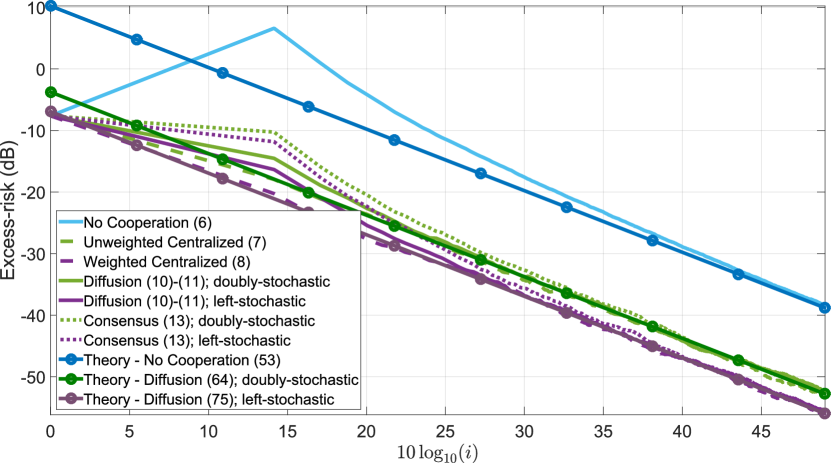
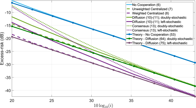
The results derived in Sec.IV apply to this definition of excess-risk, and we can therefore expect that the KL divergence curve of the diffusion strategy (10)–(11) will be below that of the consensus algorithm (13), and that the diffusion strategy will outperform both the non-cooperative solution (6) and the centralized algorithm (7).
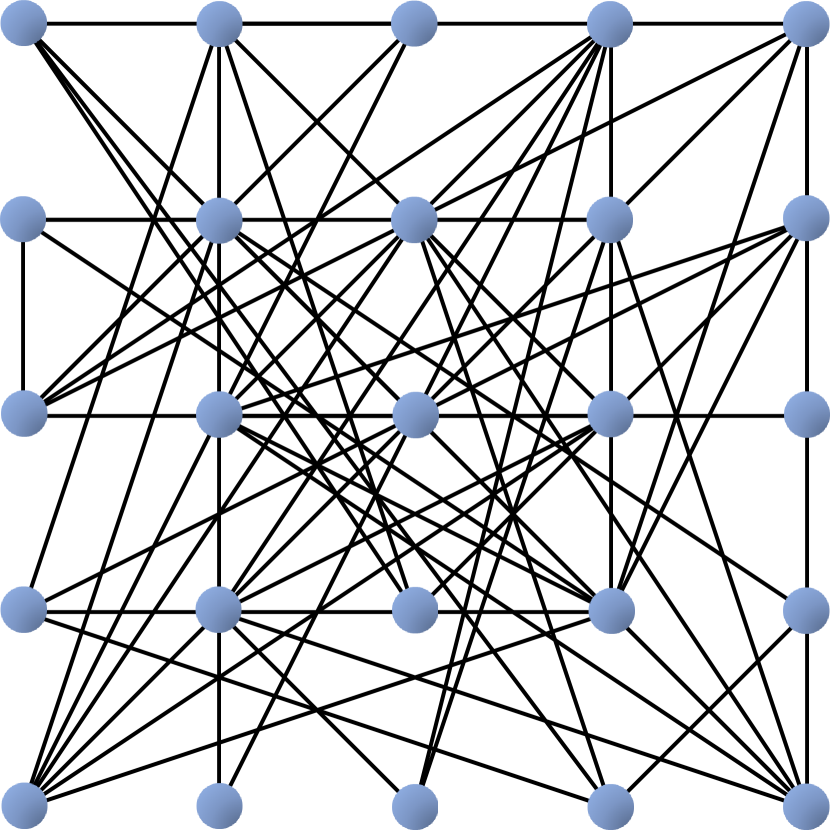
Refer to caption
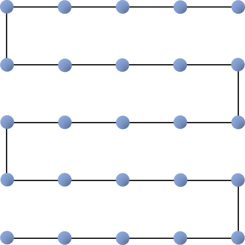
(a) The fully-connected network topology used to obtain the simulation results in Sec. V-A.
Refer to caption
(b) The sparsely-connected network topology used to obtain the simulation results in Sec. V-A.
Refer to caption
(c) The line-topology used to obtain the simulation results in Sec. V-A.
Refer to caption
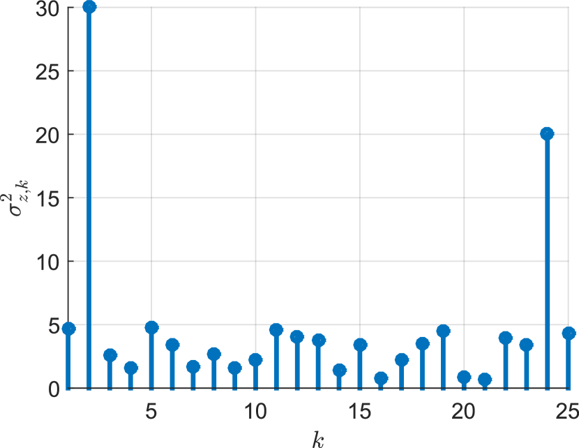
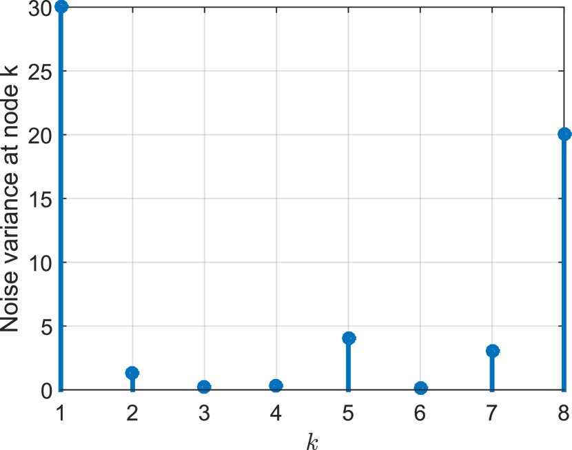
(d) Plot of noise variances across the 505050 nodes in the simulation.
Refer to caption
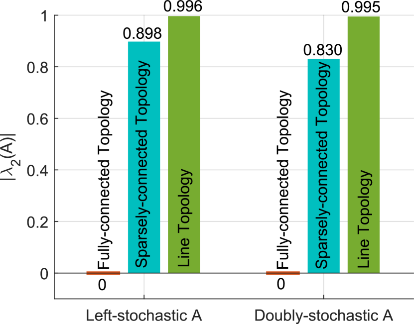
(e) Plot of the second largest eigenvalue of the combination matrices for various topologies. A fully-connected A𝐴A matrix always has a single non-zero eigenvalue at 111.
Figure 2: Simulation parameters for quadratic risk optimization: (a) The fully-connected network topology, (b) The sparsely-connected network topology, (c) The line-topology used in the simulations, (d) The noise variance at each node, and (e) The eigenvalue spectrum of the combination matrix A𝐴A.
Refer to caption
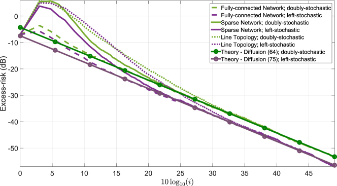
Figure 3: Simulation of the diffusion strategy for (1) a fully-connected network; (2) a sparsely-connected network; and (3) a line-topology. The network topologies and simulation parameters are listed in Fig. 2. Best viewed in color.
Refer to caption
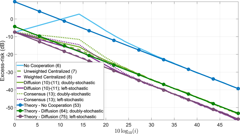
(a) Condition number of the matrix H𝐻H is 111. Comparison of non-cooperative, centralized, diffusion, and consensus strategies.
Refer to caption
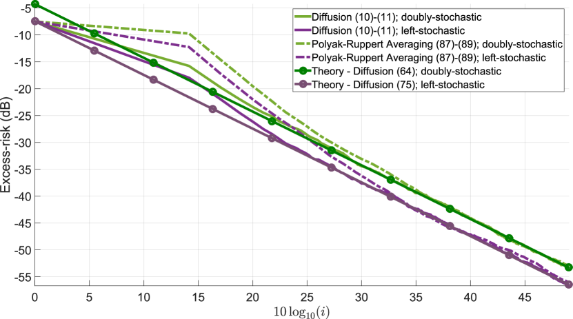
(b) Condition number of the matrix H𝐻H is 111. Comparison of non-averaged and averaged diffusion strategies.
Refer to caption
(c) Condition number of the matrix H𝐻H is 222. Comparison of non-cooperative, centralized, diffusion, and consensus strategies.
Refer to caption
(d) Condition number of the matrix H𝐻H is 222. Comparison of non-averaged and averaged diffusion strategies.
Refer to caption
(e) Condition number of the matrix H𝐻H is 444. Comparison of non-cooperative, centralized, diffusion, and consensus strategies.
Refer to caption
(f) Condition number of the matrix H𝐻H is 444. Comparison of non-averaged and averaged diffusion strategies.
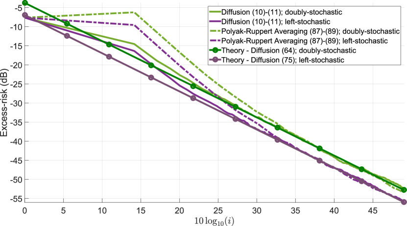
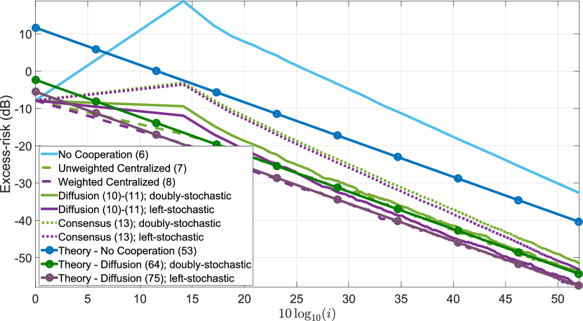
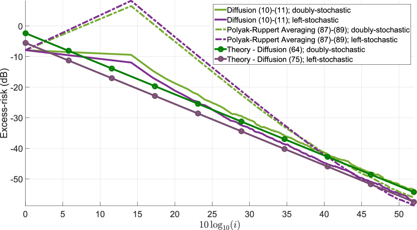
Figure 4: Comparison between learning curves of non-cooperative processing (6), diffusion algorithm (10)-(11), consensus algorithm (13), unweighted centralized (7), weighted centralized (8), and Polyak-Ruppert averaging scheme (90)–(92) for quadratic loss minimization. Best viewed in color.

We simulate the above results by considering a network with N=25𝑁25N=25 nodes as illustrated in Figs. 2(a)2(c). The quadratic loss function optimized at each node is (85), where 𝒉k,isubscript𝒉𝑘𝑖{\bm{h}}_{k,i} is a random vector in M×1superscript𝑀1\mathds{R}^{M\times 1} and M=4𝑀4M=4 and is a Gaussian random vector with i.i.d. elements and zero mean and unit variance. In addition, the scalar observation 𝒚k(i)subscript𝒚𝑘𝑖{\bm{y}}_{k}(i) is generated according to (83), where 𝒛k(i)subscript𝒛𝑘𝑖{\bm{z}}_{k}(i) is a Gaussian random variable with zero mean and variance σz,k2superscriptsubscript𝜎𝑧𝑘2\sigma_{z,k}^{2} as illustrated in Fig. 2(d). The combination weights are chosen according to the Hastings rule (63) using either the optimized Perron vector (62) or the uniform Perron vector that leads to the doubly-stochastic combination matrix p=1N𝟙N𝑝1𝑁subscript1𝑁p=\frac{1}{N}\mathds{1}_{N}. The magnitude of the second largest eigenvalue of the left- and doubly-stochastic matrices are illustrated in Fig. 2(e). The step-size was optimized via (81). Observe that we let two out of the 252525 nodes have particularly bad noise conditions. This should highlight the benefit of using left-stochastic weights as opposed to doubly-stochastic weights. The simulation results are illustrated in Fig. 4. The curves are averaged over 100100100 experiments. The network topologies examined in the simulations in this section are illustrated illustrated in Fig. 2(a)2(c).

V-A1 Asymptotic Performance invariance due to network topology

We first illustrate one of the main conclusions we draw from Theorem 2, which is that the diffusion strategy’s asymptotic performance is independent of the particular network topology. To do this, we simulate the diffusion strategy with three network topologies: (1) Fully-connected (Fig. 2(a)); (2) Sparsely-connected (Fig. 2(b)); and (3) Line topology (Fig. 2(c)). We utilize the Hastings rule (63) to obtain both left-stochastic and doubly-stochastic combination matrices by setting the desired Perron vector p𝑝p to the optimal vector (62) or 1N𝟙N1𝑁subscript1𝑁\frac{1}{N}\mathds{1}_{N}. Such combination matrices can be generated for any connected network topology. The eigen-spectrum of the resulting combination matrices for each topology are illustrated in Fig. 2(e). We observe that as the network becomes better connected, the second-largest eigenvalue is reduced. This eigen-value generally determines the convergence speed of the transient terms.

Figure 3 illustrates the simulation results for all of the simulated network topologies. We observe that regardless of the network topology, the diffusion strategy converges to the curve described by (49), albeit at different speeds. The fully-connected network case is theoretically equivalent to the centralized strategies (7) and (8), depending on the vector p𝑝p used. We conclude, therefore, that the diffusion strategy is invariant to the particular network topology and its asymptotic excess-risk curve only depends on the Perron vector of the combination matrix, which can be freely designed for connected networks.

V-A2 Performance comparisons

We now simulate the diffusion strategy as well as other algorithms discussed in the manuscript. In addition to the non-cooperative (6), diffusion (10)–(11), consensus (13), unweighted centralized (7), and weighted centralized (8) strategies, we also examine the performance of non-cooperative and distributed Polyak-Ruppert (PR) averaging strategies. The non-cooperative PR algorithm can be described as:

ϕk,isubscriptbold-italic-ϕ𝑘𝑖\displaystyle\bm{\phi}_{k,i} =ϕk,i1μ(i)wQ(ϕk,i1,𝒙k,i)absentsubscriptbold-italic-ϕ𝑘𝑖1𝜇𝑖subscript𝑤𝑄subscriptbold-italic-ϕ𝑘𝑖1subscript𝒙𝑘𝑖\displaystyle=\bm{\phi}_{k,i-1}\!-\!\mu(i)\nabla_{\!w}Q(\!\bm{\phi}_{k,i-1},\!{\bm{x}}_{k,i}\!) [adaptation]delimited-[]adaptation\displaystyle[\textrm{adaptation}] (88)
𝒘k,isubscript𝒘𝑘𝑖\displaystyle{\bm{w}}_{k,i} =𝒘k,i1+1i(ϕk,i𝒘k,i1)absentsubscript𝒘𝑘𝑖11𝑖subscriptbold-italic-ϕ𝑘𝑖subscript𝒘𝑘𝑖1\displaystyle={\bm{w}}_{k,i-1}+\frac{1}{i}\left(\bm{\phi}_{k,i}-{\bm{w}}_{k,i-1}\right) [averaging]delimited-[]averaging\displaystyle[\textrm{averaging}] (89)

which is simply the non-cooperative algorithm (6) operating independently, and a time-averaging process of the iterates to smooth the estimates. On the other hand, the distributed version that we implement for comparison takes the form:

𝝍k,isubscript𝝍𝑘𝑖\displaystyle\bm{\psi}_{k,i}\! =ϕk,i1μ(i)wQ(ϕk,i1,𝒙k,i)absentsubscriptbold-italic-ϕ𝑘𝑖1𝜇𝑖subscript𝑤𝑄subscriptbold-italic-ϕ𝑘𝑖1subscript𝒙𝑘𝑖\displaystyle=\!\bm{\phi}_{k,i-1}\!-\!\mu(i)\nabla_{w}Q(\bm{\phi}_{k,i-1},{\bm{x}}_{k,i}) [adaptation] (90)
ϕk,isubscriptbold-italic-ϕ𝑘𝑖\displaystyle\bm{\phi}_{k,i}\! ==1Nak𝝍,iabsentsuperscriptsubscript1𝑁subscript𝑎𝑘subscript𝝍𝑖\displaystyle=\!\sum_{\ell=1}^{N}a_{\ell k}\bm{\psi}_{\ell,i} [aggregation] (91)
𝒘k,isubscript𝒘𝑘𝑖\displaystyle{\bm{w}}_{k,i} =𝒘k,i1+1i(ϕk,i𝒘k,i1)absentsubscript𝒘𝑘𝑖11𝑖subscriptbold-italic-ϕ𝑘𝑖subscript𝒘𝑘𝑖1\displaystyle={\bm{w}}_{k,i-1}+\frac{1}{i}\left(\bm{\phi}_{k,i}-{\bm{w}}_{k,i-1}\right) [averaging] (92)

where the combination matrix with elements {ak}subscript𝑎𝑘\{a_{\ell k}\} is the same as the one used for the diffusion and consensus strategies.

It has been shown for single-agent stochastic approximation algorithms [22, 45, 35, 46] that the averaging operation allows the algorithm to be robust to loss of strong-convexity in the risk function (the algorithm will continue to converge at the fastest possible rate for the non-strongly-convex problem, albeit slower than the rate it would have achieved for the strongly-convex problem) in addition to achieving the best possible rate regardless of the eigen-structure of the Hessian matrix H𝐻H (which is important when H𝐻H is ill-conditioned). Unfortunately, these algorithms have also been shown to be sensitive to initialization [22] in that transient terms in their excess-risk curve decay at a relatively slow rate of 1/i21superscript𝑖21/i^{2}—in comparison to stochastic gradient descent, which forgets the initialization at a rate of 1/i2λminμ1superscript𝑖2subscript𝜆𝜇1/i^{2\lambda_{\min}\mu} asymptotically (Theorem 5), which can be made to decay faster with the choice of μ𝜇\mu, and faster in the earlier stages [22]. In addition, the step-size sequence μ(i)𝜇𝑖\mu(i) for the PR algorithms must decay slower than 1/i1𝑖1/i; for example μ(i)=μ/i2/3𝜇𝑖𝜇superscript𝑖23\mu(i)=\mu/i^{2/3}. Various methods have been suggested for avoiding such drawbacks such as to start the averaging process after some number of iterations [47] or selecting a small initial step-size μ𝜇\mu to reduce the size of the over-shoot. Unfortunately, it is usually not clear how many iterations should elapse before averaging starts. This is still a useful research direction to explore. In our simulations we use μ(i)=μ/i2/3𝜇𝑖𝜇superscript𝑖23\mu(i)=\mu/i^{2/3} as suggested in [22] for the PR averaging strategies.

The curves illustrate that the difference in performance between non-cooperative processing (6) and the diffusion algorithm with doubly-stochastic weights (i.e., the algorithm studied in [16]) is about 141414dB (10log10(N)10subscript10𝑁10\log_{10}(N)). We also observe that (10)-(11) achieves 101010dB per decade decay in simulation (1/i1𝑖1/i rate), and that the diffusion strategy with left-stochastic weights outperforms the un-weighted centralized solution (7) and the doubly-stochastic implementation. In comparison to the consensus algorithm (13), the diffusion algorithm (10)-(11) is seen to have better transient performance, and the network excess-risk for the consensus strategy remains higher than that for diffusion regardless of the combination matrix used (as predicted by Theorem 3). In addition, we observe that the left-stochastic diffusion algorithm approaches the same performance curve as the weighted centralized strategy (8) as predicted by theory.

We also observe that the Polyak-Ruppert averaging diffusion scheme exhibits worse performance than the non-averaged case when the condition number of H𝐻H is unity. This is due to the poor transient performance of the averaged algorithm [22, 48]. However, as the condition number of H𝐻H worsens, the averaged diffusion algorithm outperforms the standard diffusion scheme.

V-B Regularized Logistic Regression
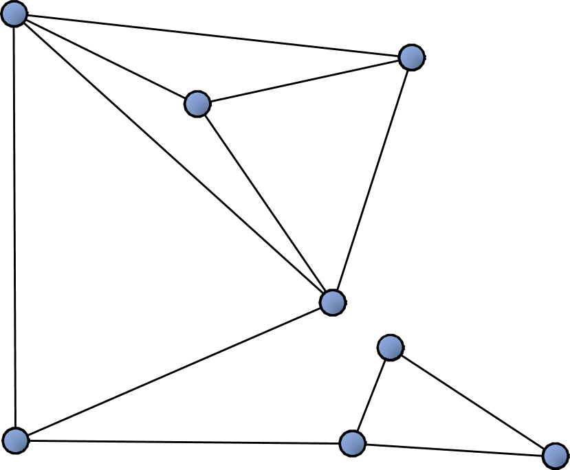
Refer to caption
(a) Network topology used to obtain the simulation results in Sec. V-B.
Refer to caption
(b) Plot of noise variances across the 888 nodes in the simulation.
Refer to caption
(c) Regularized KL divergence attained by nodes that utilize the non-cooperative algorithm (6), the unweighted centralized algorithm (7), the weighted centralized algorithm (8), the diffusion strategy (10)-(11), and consensus strategy (13) with optimized weights (62) and with doubly-stochastic weights (p=1N𝟙N𝑝1𝑁subscript1𝑁p=\frac{1}{N}\mathds{1}_{N}). Theoretical curves are from (57), (66) and (68). Curves are averaged over 200020002000 experiments.
Figure 5: Plot of the simulation parameters and results for the regularized logistic regression simulation.

Now consider an application where the dependent variable 𝒚k(i)subscript𝒚𝑘𝑖{\bm{y}}_{k}(i) is binary (i.e, it assumes values from the set {+1,1}11\{+1,-1\}) with 𝒉k,M×1subscript𝒉𝑘superscript𝑀1{\bm{h}}_{k,}\in\mathbb{R}^{M\times 1}. The log-odds function is assumed to obey the linear model [49, p. 117]:

log(p(𝒚k(i)|𝒉k,i;w)1p(𝒚k(i)|𝒉k,i;w))=𝒚k(i)𝒉k,i𝖳w𝑝conditionalsubscript𝒚𝑘𝑖subscript𝒉𝑘𝑖𝑤1𝑝conditionalsubscript𝒚𝑘𝑖subscript𝒉𝑘𝑖𝑤subscript𝒚𝑘𝑖superscriptsubscript𝒉𝑘𝑖𝖳𝑤\displaystyle\log\left(\frac{p({\bm{y}}_{k}(i)|{\bm{h}}_{k,i};w)}{1-p({\bm{y}}_{k}(i)|{\bm{h}}_{k,i};w)}\right)={\bm{y}}_{k}(i){\bm{h}}_{k,i}^{\mathsf{T}}w (93)

Solving for p(𝒚k,i|𝒉k,i;w)𝑝conditionalsubscript𝒚𝑘𝑖subscript𝒉𝑘𝑖𝑤p({\bm{y}}_{k,i}|{\bm{h}}_{k,i};w), we have that the likelihood is given by

p(𝒚k(i)|𝒉k,i;w)=11+e𝒚k(i)𝒉k,i𝖳w𝑝conditionalsubscript𝒚𝑘𝑖subscript𝒉𝑘𝑖𝑤11superscript𝑒subscript𝒚𝑘𝑖superscriptsubscript𝒉𝑘𝑖𝖳𝑤\displaystyle p({\bm{y}}_{k}(i)|{\bm{h}}_{k,i};w)=\frac{1}{1+e^{-{\bm{y}}_{k}(i){\bm{h}}_{k,i}^{\mathsf{T}}w}} (94)

Then, the maximum-likelihood estimate of wosuperscript𝑤𝑜w^{o} minimizes the negative log-likelihood function:

Q(w,𝒉k,i,𝒚k(i))=log(1+e𝒚k(i)𝒉k,i𝖳w)𝑄𝑤subscript𝒉𝑘𝑖subscript𝒚𝑘𝑖1superscript𝑒subscript𝒚𝑘𝑖superscriptsubscript𝒉𝑘𝑖𝖳𝑤\displaystyle Q(w,{\bm{h}}_{k,i},{\bm{y}}_{k}(i))=\log\left(1+e^{-{\bm{y}}_{k}(i){\bm{h}}_{k,i}^{\mathsf{T}}w}\right) (95)

Observe that Q(w,𝒉k,i,𝒚k(i))𝑄𝑤subscript𝒉𝑘𝑖subscript𝒚𝑘𝑖Q(w,{\bm{h}}_{k,i},{\bm{y}}_{k}(i)) is not strongly-convex. In order to alleviate this difficulty, it is possible to add a small regularizer so that [50, 51]:

Q(w,𝒉k,i,𝒚k(i))=ρ2w2+log(1+e𝒚k(i)𝒉k,i𝖳w)𝑄𝑤subscript𝒉𝑘𝑖subscript𝒚𝑘𝑖𝜌2superscriptnorm𝑤21superscript𝑒subscript𝒚𝑘𝑖superscriptsubscript𝒉𝑘𝑖𝖳𝑤\displaystyle Q(w,{\bm{h}}_{k,i},{\bm{y}}_{k}(i))=\frac{\rho}{2}\|w\|^{2}+\log\left(1+e^{-{\bm{y}}_{k}(i){\bm{h}}_{k,i}^{\mathsf{T}}w}\right) (96)

and the excess-risk then has the interpretation of being the regularized KL divergence:

DRKLsubscript𝐷RKL\displaystyle D_{\textrm{RKL}} (p(𝒚k(i)|𝒉k,i;wo)p(𝒚k(i)|𝒉k,i;w))\displaystyle\big{(}p({\bm{y}}_{k}(i)|{\bm{h}}_{k,i};w^{o})\parallel p({\bm{y}}_{k}(i)|{\bm{h}}_{k,i};w)\big{)}
ρ2(w2wo2)+𝔼{log(p(𝒚k(i)|𝒉k,i;wo)p(𝒚k(i)|𝒉k,i;w))}absent𝜌2superscriptnorm𝑤2superscriptnormsuperscript𝑤𝑜2𝔼𝑝conditionalsubscript𝒚𝑘𝑖subscript𝒉𝑘𝑖superscript𝑤𝑜𝑝conditionalsubscript𝒚𝑘𝑖subscript𝒉𝑘𝑖𝑤\displaystyle\triangleq\frac{\rho}{2}\left(\|w\|^{2}\!-\!\|w^{o}\|^{2}\right)+{\mathbb{E}}\left\{\log\left(\frac{p({\bm{y}}_{k}(i)|{\bm{h}}_{k,i};w^{o})}{p({\bm{y}}_{k}(i)|{\bm{h}}_{k,i};w)}\right)\right\} (97)

We generate a random adhoc network of N=8𝑁8N=8 nodes (illustrated in Fig. 5(a)) where each node samples M=2𝑀2M=2 dimensional feature vectors from a Gaussian mixture with two components and probability density function 𝒉k,i12𝒩(2𝟙,IM)+12𝒩(2𝟙,IM)similar-tosubscript𝒉𝑘𝑖12𝒩21subscript𝐼𝑀12𝒩21subscript𝐼𝑀{\bm{h}}_{k,i}\sim\frac{1}{2}\mathcal{N}(2\mathds{1},I_{M})+\frac{1}{2}\mathcal{N}(-2\mathds{1},I_{M}), where 𝒩(γ,Σ)𝒩𝛾Σ\mathcal{N}(\gamma,\Sigma) denotes the multivariate Gaussian density function with mean vector γ𝛾\gamma and covariance matrix ΣΣ\Sigma. The labels 𝒚k(i)subscript𝒚𝑘𝑖{\bm{y}}_{k}(i) are generated according to

p(𝒚k(i)|𝒉k,i;wo)=11+e𝒚k(i)𝒉k,i𝖳wo𝑝conditionalsubscript𝒚𝑘𝑖subscript𝒉𝑘𝑖superscript𝑤𝑜11superscript𝑒subscript𝒚𝑘𝑖superscriptsubscript𝒉𝑘𝑖𝖳superscript𝑤𝑜\displaystyle p({\bm{y}}_{k}(i)|{\bm{h}}_{k,i};w^{o})=\frac{1}{1+e^{-{\bm{y}}_{k}(i){\bm{h}}_{k,i}^{\mathsf{T}}w^{o}}} (98)

where wosuperscript𝑤𝑜w^{o} is chosen arbitrary at the start of each experiment. Each node performs the diffusion algorithm listed in (10)-(11) by computing the gradient according to the instantaneous approximation of the strongly-convex regularized KL divergence (97). Since in this scenario, the noise profile is uniform across the agents, the optimal weights (62) become po=1N𝟙Nsuperscript𝑝𝑜1𝑁subscript1𝑁p^{o}=\frac{1}{N}\mathds{1}_{N}, which leads to a doubly-stochastic combination policy, A𝐴A. In order to simulate a scenario involving a left-stochastic combination rule, we modify the instantaneous approximations for the gradient vectors across the agents by adding a small additive noise component to these approximations at each agent with varying power profile shown in Fig. (5(b)). These noise perturbations help model unknown effects or even round-off errors.

The regularization constant ρ𝜌\rho is chosen to be 555 in the simulation since it will determine λminsubscript𝜆\lambda_{\min} and in order to ensure that our approximation in (66) is valid, we choose μ𝜇\mu to be 555. The optimizer is found by optimizing the sum of the regularized KL divergences and using empirical average for the expectation.

Figure 5(c) shows the resulting curves, which are averaged over 500500500 experiments (with a different random network topology per experiment). We plot the performance of the non-cooperative algorithm along with its theoretical performance (both averaged over the nodes). In addition, we show the performance of the centralized algorithms (7) and (8) along with their theoretical performance obtained from the right-hand-side of (68) and (79). We see that the diffusion algorithm outperforms the non-cooperative algorithm and matches the centralized algorithm listed in (7) when the combination policy A𝐴A is doubly-stochastic, as predicted by Theorem 2. We also observe that when A𝐴A is chosen to be left-stochastic, the diffusion strategy outperforms (7), as predicted by (76) and approaches to same performance as the weighted centralized algorithm (8), as expected.

VI Conclusions and Future Work

We performed a detailed mean-square-error analysis of the asymptotic convergence behavior of distributed strategies of the consensus and diffusion types. We established that the algorithms converge asymptotically at the rate of O(1/i)𝑂1𝑖O(1/i) and, more importantly, derived the exact constant that multiplies the convergence rate factor 1/i1𝑖1/i. By using the derived expressions, we were able to compare the performance of various implementations against each other including non-cooperative strategies, centralized strategies, and distributed consensus and diffusion strategies. The analysis revealed that diffusion implementations outperform the other strategies and deliver the best excess-risk performance asymptotically as centralized strategies; we also showed how to optimize this performance over the choice of combination weights. We showed that the optimal weights are left-stochastic rather than doubly-stochastic and derived an expression for them in terms of the Hastings rule. We also observed that the diffusion implementation leads to smaller overshoot during the transient phase in relation to the other strategies in simulations. It was also demonstrated that the asymptotic performance of the difusion strategy is independent of the particular network topology that connects the agents. The analysis in this work was done under the assumption of stationary data distributions, in which case decaying step-sizes are justified. If the statistical distribution of the data drifts with time, then constant step-sizes need to be employed. In this case, the dynamics of the learning network is modified in one important way in that the gradient noise does not die out anymore (it is annihilated by decaying step-sizes but not by constant step-sizes). The performance of the networks in the constant step-size regime is studied in [32, 34, 14, 15]. A useful extension of this work is to study the Polyak-Ruppert averaging version (90)–(92) for robustness against ill-conditioning and lack of strong-convexity.

Appendix A Proof of Theorem 1

We denote the error vectors at node k𝑘k at time i𝑖i by 𝝍~k,iwo𝝍k,isubscript~𝝍𝑘𝑖superscript𝑤𝑜subscript𝝍𝑘𝑖\tilde{{\bm{\psi}}}_{k,i}\triangleq w^{o}-{\bm{\psi}}_{k,i} and 𝒘~k,iwo𝒘k,isubscript~𝒘𝑘𝑖superscript𝑤𝑜subscript𝒘𝑘𝑖\widetilde{{\bm{w}}}_{k,i}\triangleq w^{o}-{\bm{w}}_{k,i}. We subtract (10)-(11) from wosuperscript𝑤𝑜w^{o} using (23) to get

𝝍~k,isubscript~𝝍𝑘𝑖\displaystyle\tilde{{\bm{\psi}}}_{k,i} =𝒘~k,i1+μ(i)[wJk(𝒘k,i1)+𝒗k,i(𝒘k,i1)]absentsubscript~𝒘𝑘𝑖1𝜇𝑖delimited-[]subscript𝑤subscript𝐽𝑘subscript𝒘𝑘𝑖1subscript𝒗𝑘𝑖subscript𝒘𝑘𝑖1\displaystyle=\widetilde{{\bm{w}}}_{k,i-1}\!+\!\mu(i)\left[\nabla_{w}J_{k}({\bm{w}}_{k,i-1})\!+\!{\bm{v}}_{k,i}({\bm{w}}_{k,i-1})\right] (99)
𝒘~k,isubscript~𝒘𝑘𝑖\displaystyle\widetilde{{\bm{w}}}_{k,i} ==1Nak𝝍~,iabsentsuperscriptsubscript1𝑁subscript𝑎𝑘subscript~𝝍𝑖\displaystyle=\sum_{\ell=1}^{N}a_{\ell k}\tilde{{\bm{\psi}}}_{\ell,i} (100)

Using the mean-value relation (22), we can write

wJk(𝒘k,i1)=𝑯k,i𝒘~k,i1subscript𝑤subscript𝐽𝑘subscript𝒘𝑘𝑖1subscript𝑯𝑘𝑖subscript~𝒘𝑘𝑖1\displaystyle\nabla_{w}J_{k}({\bm{w}}_{k,i-1})=-{\bm{H}}_{k,i}\widetilde{{\bm{w}}}_{k,i-1} (101)

where

𝑯k,i01w2Jk(wot𝒘~k,i1)𝑑tsubscript𝑯𝑘𝑖superscriptsubscript01subscriptsuperscript2𝑤subscript𝐽𝑘superscript𝑤𝑜𝑡subscript~𝒘𝑘𝑖1differential-d𝑡{\bm{H}}_{k,i}\!\triangleq\!\int_{0}^{1}\nabla^{2}_{w}J_{k}(w^{o}\!-\!t\widetilde{{\bm{w}}}_{k,i-1})dt (102)

and where we used the fact that wJk(wo)=0subscript𝑤subscript𝐽𝑘superscript𝑤𝑜0\nabla_{w}J_{k}(w^{o})=0 since wosuperscript𝑤𝑜w^{o} optimizes Jk(w)subscript𝐽𝑘𝑤J_{k}(w). Substituting (101) into (99), we get

𝝍~k,isubscript~𝝍𝑘𝑖\displaystyle\tilde{{\bm{\psi}}}_{k,i} =[Iμ(i)𝑯k,i1]𝒘~k,i1+μ(i)𝒗k,i(𝒘k,i1)absentdelimited-[]𝐼𝜇𝑖subscript𝑯𝑘𝑖1subscript~𝒘𝑘𝑖1𝜇𝑖subscript𝒗𝑘𝑖subscript𝒘𝑘𝑖1\displaystyle=\left[I-\mu(i){\bm{H}}_{k,i-1}\right]\widetilde{{\bm{w}}}_{k,i-1}+\mu(i){\bm{v}}_{k,i}({\bm{w}}_{k,i-1}) (103)

We now derive mean-square-error (MSE) recursions by noting that x2x𝖳xsuperscriptnorm𝑥2superscript𝑥𝖳𝑥\|x\|^{2}\triangleq x^{\mathsf{T}}x is a convex function of x𝑥x. Therefore, applying Jensen’s inequality [52, p. 77] to (100) we obtain:

𝔼{𝒘~k,i2|𝓕i1}𝔼conditionalsuperscriptnormsubscript~𝒘𝑘𝑖2subscript𝓕𝑖1\displaystyle\mathbb{E}\{\|\widetilde{{\bm{w}}}_{k,i}\|^{2}|\bm{\mathcal{F}}_{i-1}\} =1Nak𝔼{𝝍~,i2|𝓕i1}absentsuperscriptsubscript1𝑁subscript𝑎𝑘𝔼conditionalsuperscriptnormsubscript~𝝍𝑖2subscript𝓕𝑖1\displaystyle\leq\sum_{\ell=1}^{N}a_{\ell k}\mathbb{E}\{\|\tilde{{\bm{\psi}}}_{\ell,i}\|^{2}|\bm{\mathcal{F}}_{i-1}\} (104)

for k=1,,N𝑘1𝑁k=1,\ldots,N. From (103) and using Assumption 2, we get

𝔼{𝝍~k,i2\displaystyle\mathbb{E}\{\|\tilde{{\bm{\psi}}}_{k,i}\|^{2} |𝓕i1}=𝔼{𝒘~k,i1𝚺k,i2|𝓕i1}+\displaystyle|\bm{\mathcal{F}}_{i-1}\}=\mathbb{E}\{\|\widetilde{{\bm{w}}}_{k,i-1}\|^{2}_{{\bm{\Sigma}}_{k,i}}|\bm{\mathcal{F}}_{i-1}\}+
μ2(i)𝔼{𝒗k,i(𝒘k,i1)2|𝓕i1}superscript𝜇2𝑖𝔼conditionalsuperscriptnormsubscript𝒗𝑘𝑖subscript𝒘𝑘𝑖12subscript𝓕𝑖1\displaystyle\mu^{2}(i)\cdot{\mathbb{E}}\{\left\|{\bm{v}}_{k,i}({\bm{w}}_{k,i-1})\right\|^{2}|\bm{\mathcal{F}}_{i-1}\} (105)

where 𝚺k,i(IMμ(i)𝑯k,i1)2subscript𝚺𝑘𝑖superscriptsubscript𝐼𝑀𝜇𝑖subscript𝑯𝑘𝑖12{\bm{\Sigma}}_{k,i}\triangleq\left(I_{M}-\mu(i){\bm{H}}_{k,i-1}\right)^{2}. The matrices 𝚺k,isubscript𝚺𝑘𝑖{\bm{\Sigma}}_{k,i} can be seen to be positive semi-definite for large enough i𝑖i and bounded by

0𝚺k,iγ2(i)IM0subscript𝚺𝑘𝑖superscript𝛾2𝑖subscript𝐼𝑀\displaystyle 0\leq{\bm{\Sigma}}_{k,i}\leq\gamma^{2}(i)I_{M} (106)

where

γ(i)max{|1μ(i)λ¯|,|1μ(i)λ¯|}𝛾𝑖1𝜇𝑖¯𝜆1𝜇𝑖¯𝜆\displaystyle\gamma(i)\triangleq\max\left\{\left|1-\mu(i)\bar{\lambda}\right|,\left|1-\mu(i)\underline{\lambda}\right|\right\} (107)

Now note that γ2(i)superscript𝛾2𝑖\gamma^{2}(i) can be upper-bounded by:

γ2(i)superscript𝛾2𝑖\displaystyle\gamma^{2}(i) =max{12μ(i)λ¯+μ2(i)λ¯2,12μ(i)λ¯+μ2(i)λ¯2}absent12𝜇𝑖¯𝜆superscript𝜇2𝑖superscript¯𝜆212𝜇𝑖¯𝜆superscript𝜇2𝑖superscript¯𝜆2\displaystyle=\max\left\{1-2\mu(i)\bar{\lambda}+\mu^{2}(i)\bar{\lambda}^{2},1-2\mu(i)\underline{\lambda}+\mu^{2}(i)\underline{\lambda}^{2}\right\}
12μ(i)λ¯+μ2(i)λ¯2absent12𝜇𝑖¯𝜆superscript𝜇2𝑖superscript¯𝜆2\displaystyle\leq 1-2\mu(i)\underline{\lambda}+\mu^{2}(i)\bar{\lambda}^{2} (108)

In order to simplify the notation, we introduce the upper-bound

β(i)𝛽𝑖\displaystyle\beta(i) 12μ(i)λ¯(1(λ¯2+α2)2λ¯μ(i))absent12𝜇𝑖¯𝜆1superscript¯𝜆2subscript𝛼22¯𝜆𝜇𝑖\displaystyle\triangleq 1-2\mu(i)\underline{\lambda}\left(1-\frac{(\bar{\lambda}^{2}+\alpha_{2})}{2\underline{\lambda}}\mu(i)\right) (109)

where α2subscript𝛼2\alpha_{2} is defined by (33), namely,

𝔼{𝒗k,i(𝒘k,i1)2|𝓕i1}α2𝒘~k,i12+σv22𝔼conditionalsuperscriptnormsubscript𝒗𝑘𝑖subscript𝒘𝑘𝑖12subscript𝓕𝑖1subscript𝛼2superscriptnormsubscript~𝒘𝑘𝑖12superscriptsubscript𝜎𝑣22\displaystyle{\mathbb{E}}\{\left\|{\bm{v}}_{k,i}({\bm{w}}_{k,i-1})\right\|^{2}|\bm{\mathcal{F}}_{i-1}\}\leq\alpha_{2}\|\widetilde{{\bm{w}}}_{k,i-1}\|^{2}+\sigma_{v2}^{2} (110)

Combining (105), (106), and (110), we obtain for k=1,,N𝑘1𝑁k=1,\ldots,N:

𝔼{𝝍~k,i2|𝓕i1}𝔼conditionalsuperscriptnormsubscript~𝝍𝑘𝑖2subscript𝓕𝑖1\displaystyle\mathbb{E}\{\|\tilde{{\bm{\psi}}}_{k,i}\|^{2}|\bm{\mathcal{F}}_{i-1}\} β(i)𝒘~k,i12+μ2(i)σv22absent𝛽𝑖superscriptnormsubscript~𝒘𝑘𝑖12superscript𝜇2𝑖superscriptsubscript𝜎𝑣22\displaystyle\leq\beta(i)\,\|\widetilde{{\bm{w}}}_{k,i-1}\|^{2}+\mu^{2}(i)\sigma_{v2}^{2} (111)

We introduce the MSE vectors:

𝓦isubscript𝓦𝑖\displaystyle\bm{\mathcal{W}}_{i} [𝒘~1,i2,,𝒘~N,i2]𝖳absentsuperscriptsuperscriptnormsubscript~𝒘1𝑖2superscriptnormsubscript~𝒘𝑁𝑖2𝖳\displaystyle\triangleq\big{[}\|\widetilde{{\bm{w}}}_{1,i}\|^{2},\dots,\|\widetilde{{\bm{w}}}_{N,i}\|^{2}\big{]}^{\mathsf{T}} (112)
𝓨isubscript𝓨𝑖\displaystyle\bm{\mathcal{Y}}_{i} [𝝍~1,i2,,𝝍~N,i2]𝖳absentsuperscriptsuperscriptnormsubscript~𝝍1𝑖2superscriptnormsubscript~𝝍𝑁𝑖2𝖳\displaystyle\triangleq\big{[}\|\tilde{{\bm{\psi}}}_{1,i}\|^{2},\dots,\|\tilde{{\bm{\psi}}}_{N,i}\|^{2}\big{]}^{\mathsf{T}} (113)

and rewrite (104), and (111) as:

𝔼{𝓨i|𝓕i1}𝔼conditional-setsubscript𝓨𝑖subscript𝓕𝑖1\displaystyle{\mathbb{E}}\{\bm{\mathcal{Y}}_{i}|\bm{\mathcal{F}}_{i-1}\} β(i)𝓦i1+μ2(i)σv22𝟙Nprecedes-or-equalsabsent𝛽𝑖subscript𝓦𝑖1superscript𝜇2𝑖superscriptsubscript𝜎𝑣22subscript1𝑁\displaystyle\preceq\beta(i)\bm{\mathcal{W}}_{i-1}+\mu^{2}(i)\sigma_{v2}^{2}\mathds{1}_{N} (114)
𝔼{𝓦i|𝓕i1}𝔼conditional-setsubscript𝓦𝑖subscript𝓕𝑖1\displaystyle{\mathbb{E}}\{\bm{\mathcal{W}}_{i}|\bm{\mathcal{F}}_{i-1}\} A𝖳𝔼{𝓨i|𝓕i1}precedes-or-equalsabsentsuperscript𝐴𝖳𝔼conditional-setsubscript𝓨𝑖subscript𝓕𝑖1\displaystyle\preceq A^{\mathsf{T}}{\mathbb{E}}\{\bm{\mathcal{Y}}_{i}|\bm{\mathcal{F}}_{i-1}\} (115)

where xyprecedes-or-equals𝑥𝑦x\preceq y indicates that each element of the vector x𝑥x is less than or equal to the corresponding element of vector y𝑦y. Using the fact that if xyprecedes-or-equals𝑥𝑦x\preceq y then BxByprecedes-or-equals𝐵𝑥𝐵𝑦Bx\preceq By for any matrix B𝐵B with non-negative entries, we can combine the above inequality recursions into a single recursion for 𝒲isubscript𝒲𝑖\mathcal{W}_{i}:

𝔼{𝓦i|𝓕i1}𝔼conditional-setsubscript𝓦𝑖subscript𝓕𝑖1\displaystyle{\mathbb{E}}\{\bm{\mathcal{W}}_{i}|\bm{\mathcal{F}}_{i-1}\} β(i)A𝖳𝓦i1+μ2(i)σv22𝟙Nprecedes-or-equalsabsent𝛽𝑖superscript𝐴𝖳subscript𝓦𝑖1superscript𝜇2𝑖superscriptsubscript𝜎𝑣22subscript1𝑁\displaystyle\preceq\beta(i)A^{\mathsf{T}}\bm{\mathcal{W}}_{i-1}+\mu^{2}(i)\sigma_{v2}^{2}\mathds{1}_{N} (116)

Now, we multiply both sides by p𝖳superscript𝑝𝖳p^{\mathsf{T}}, where p𝑝p is the Perron eigenvector of A𝐴A. This yields the recursion:

𝔼{p𝖳𝓦i|𝓕i1}𝔼conditional-setsuperscript𝑝𝖳subscript𝓦𝑖subscript𝓕𝑖1\displaystyle{\mathbb{E}}\{p^{\mathsf{T}}\bm{\mathcal{W}}_{i}|\bm{\mathcal{F}}_{i-1}\} β(i)p𝖳𝓦i1+μ2(i)σv22absent𝛽𝑖superscript𝑝𝖳subscript𝓦𝑖1superscript𝜇2𝑖superscriptsubscript𝜎𝑣22\displaystyle\leq\beta(i)p^{\mathsf{T}}\bm{\mathcal{W}}_{i-1}+\mu^{2}(i)\sigma_{v2}^{2} (117)

A-A MSE Convergence

For the first part of Theorem 1 (asymptotic MSE convergence), we evaluate the expectation of both sides of the inequality in (117) to get

𝔼{p𝖳𝓦i}𝔼superscript𝑝𝖳subscript𝓦𝑖\displaystyle{\mathbb{E}}\{p^{\mathsf{T}}\bm{\mathcal{W}}_{i}\} β(i)𝔼{p𝖳𝓦i1}+μ2(i)σv22absent𝛽𝑖𝔼superscript𝑝𝖳subscript𝓦𝑖1superscript𝜇2𝑖superscriptsubscript𝜎𝑣22\displaystyle\leq\beta(i){\mathbb{E}}\{p^{\mathsf{T}}\bm{\mathcal{W}}_{i-1}\}\!+\!\mu^{2}(i)\sigma_{v2}^{2} (118)

Now since μ(i)0𝜇𝑖0\mu(i)\rightarrow 0, we conclude that for large enough i>io𝑖subscript𝑖𝑜i>i_{o}, the sequence μ2(i)superscript𝜇2𝑖\mu^{2}(i) will assume smaller values than μ(i)𝜇𝑖\mu(i). Therefore, a large enough time index, io>0subscript𝑖𝑜0i_{o}>0 exists such that the following condition is satisfied:

0<(1β(i))=(2μ(i)λ¯+(λ¯2+α2)μ2(i))<101𝛽𝑖2𝜇𝑖¯𝜆superscript¯𝜆2subscript𝛼2superscript𝜇2𝑖1\displaystyle 0<(1-\beta(i))=(2\mu(i)\underline{\lambda}+(\bar{\lambda}^{2}+\alpha_{2})\mu^{2}(i))<1 (119)

Furthermore, noting that i=1(1β(i))=superscriptsubscript𝑖11𝛽𝑖\sum_{i=1}^{\infty}(1\!-\!\beta(i))=\infty, limiμ2(i)σv22/(1β(i))=0subscript𝑖superscript𝜇2𝑖superscriptsubscript𝜎𝑣221𝛽𝑖0\lim_{i\rightarrow\infty}\mu^{2}(i)\sigma_{v2}^{2}/(1-\beta(i))=0, we then invoke Lemma 4 (Appendix G) to arrive at the desired result.

A-B Almost-Sure Convergence

We see that (117) fits the form of Lemma 6 (Appendix G), where (119) will hold for large enough i𝑖i, i=1(1β(i))=superscriptsubscript𝑖11𝛽𝑖\sum_{i=1}^{\infty}(1\!-\!\beta(i))=\infty, limiμ2(i)σv22/(1β(i))=0subscript𝑖superscript𝜇2𝑖superscriptsubscript𝜎𝑣221𝛽𝑖0\lim_{i\rightarrow\infty}\mu^{2}(i)\sigma_{v2}^{2}/(1-\beta(i))=0, and i=1μ2(i)σv22<superscriptsubscript𝑖1superscript𝜇2𝑖superscriptsubscript𝜎𝑣22\sum_{i=1}^{\infty}\mu^{2}(i)\sigma_{v2}^{2}<\infty, and we conclude that p𝖳𝓦i0superscript𝑝𝖳subscript𝓦𝑖0p^{\mathsf{T}}\bm{\mathcal{W}}_{i}\rightarrow 0 almost surely so 𝓦i0subscript𝓦𝑖0\bm{\mathcal{W}}_{i}\rightarrow 0 almost surely as well since all the entries of p𝑝p are strictly positive. This implies that 𝒘k,iwosubscript𝒘𝑘𝑖superscript𝑤𝑜{\bm{w}}_{k,i}\rightarrow w^{o} almost surely for all k=1,,N𝑘1𝑁k=1,\ldots,N.

A-C MSE Convergence Rate

For the convergence rate, we take the expectation of

𝔼{p𝖳𝓦i|𝓕i1}𝔼conditional-setsuperscript𝑝𝖳subscript𝓦𝑖subscript𝓕𝑖1\displaystyle{\mathbb{E}}\{p^{\mathsf{T}}\bm{\mathcal{W}}_{i}|\bm{\mathcal{F}}_{i-1}\} β(i)p𝖳𝓦i1+μ2(i)σv22absent𝛽𝑖superscript𝑝𝖳subscript𝓦𝑖1superscript𝜇2𝑖superscriptsubscript𝜎𝑣22\displaystyle\leq\beta(i)p^{\mathsf{T}}\bm{\mathcal{W}}_{i-1}+\mu^{2}(i)\sigma_{v2}^{2} (120)

to get

𝔼{p𝖳𝓦i}𝔼superscript𝑝𝖳subscript𝓦𝑖\displaystyle{\mathbb{E}}\{p^{\mathsf{T}}\bm{\mathcal{W}}_{i}\} (1ai+bi2)𝔼{p𝖳𝓦i1}+ci2absent1𝑎𝑖𝑏superscript𝑖2𝔼superscript𝑝𝖳subscript𝓦𝑖1𝑐superscript𝑖2\displaystyle\leq\left(1-\frac{a}{i}+\frac{b}{i^{2}}\right){\mathbb{E}}\{p^{\mathsf{T}}\bm{\mathcal{W}}_{i-1}\}+\frac{c}{i^{2}} (121)

where a2μλ¯𝑎2𝜇¯𝜆a\triangleq 2\mu\underline{\lambda}, bμ2(λ¯+α2)𝑏superscript𝜇2¯𝜆subscript𝛼2b\triangleq\mu^{2}(\bar{\lambda}+\alpha_{2}), and cσv22μ2𝑐superscriptsubscript𝜎𝑣22superscript𝜇2c\triangleq\sigma_{v2}^{2}\mu^{2}. Using Lemma 5 (Appendix G), we have that when a=2λ¯μ>1𝑎2¯𝜆𝜇1a=2\underline{\lambda}\mu>1,

lim supi𝔼{p𝖳𝓦i}i1ca1,subscriptlimit-supremum𝑖𝔼superscript𝑝𝖳subscript𝓦𝑖superscript𝑖1𝑐𝑎1\displaystyle\limsup_{i\rightarrow\infty}\frac{{\mathbb{E}}\{p^{\mathsf{T}}\bm{\mathcal{W}}_{i}\}}{i^{-1}}\leq\frac{c}{a-1}, (122)

which in turn implies that each 𝔼𝒘k,i2𝔼superscriptnormsubscript𝒘𝑘𝑖2{\mathbb{E}}\|{\bm{w}}_{k,i}\|^{2} diminishes at the rate i1superscript𝑖1i^{-1}, which is our desired result.

A-D Fourth-Order-Moment Convergence Rate

Observe that by Jensen’s inequality, we have that

𝔼𝒘~k,i4=1Nak𝔼𝝍~,i4𝔼superscriptnormsubscript~𝒘𝑘𝑖4superscriptsubscript1𝑁subscript𝑎𝑘𝔼superscriptnormsubscript~𝝍𝑖4\displaystyle{\mathbb{E}}\|\widetilde{{\bm{w}}}_{k,i}\|^{4}\leq\sum_{\ell=1}^{N}a_{\ell k}{\mathbb{E}}\|\tilde{{\bm{\psi}}}_{\ell,i}\|^{4} (123)

and

𝝍~k,i4=(IMμ(i)𝑯k,i1)𝒘~k,i1+μ(i)𝒗k,i(𝒘k,i1)4superscriptnormsubscript~𝝍𝑘𝑖4superscriptnormsubscript𝐼𝑀𝜇𝑖subscript𝑯𝑘𝑖1subscript~𝒘𝑘𝑖1𝜇𝑖subscript𝒗𝑘𝑖subscript𝒘𝑘𝑖14\displaystyle\|\tilde{{\bm{\psi}}}_{k,i}\|^{4}=\|(I_{M}\!-\!\mu(i){\bm{H}}_{k,i-1})\widetilde{{\bm{w}}}_{k,i-1}\!+\!\mu(i){\bm{v}}_{k,i}({\bm{w}}_{k,i-1})\|^{4} (124)

By utilizing Lemma 5 from [53, p. 32], we obtain:

𝔼{\displaystyle{\mathbb{E}}\{\| 𝝍~k,i4|𝓕i1}θ1(i)𝒘~k,i14+\displaystyle\tilde{{\bm{\psi}}}_{k,i}\|^{4}|\bm{\mathcal{F}}_{i-1}\}\leq\theta_{1}(i)\|\widetilde{{\bm{w}}}_{k,i-1}\|^{4}+
3μ4(i)𝔼{𝒗k,i(𝒘k,i1)4|𝓕i1}+limit-from3superscript𝜇4𝑖𝔼conditionalsuperscriptnormsubscript𝒗𝑘𝑖subscript𝒘𝑘𝑖14subscript𝓕𝑖1\displaystyle\quad\ 3\mu^{4}(i){\mathbb{E}}\{\|{\bm{v}}_{k,i}({\bm{w}}_{k,i-1})\|^{4}|\bm{\mathcal{F}}_{i-1}\}+
8θ2(i)𝒘~k,i12𝔼{𝒗k,i(𝒘k,i1)2|𝓕i1}8subscript𝜃2𝑖superscriptnormsubscript~𝒘𝑘𝑖12𝔼conditionalsuperscriptnormsubscript𝒗𝑘𝑖subscript𝒘𝑘𝑖12subscript𝓕𝑖1\displaystyle\quad\ 8\theta_{2}(i)\|\widetilde{{\bm{w}}}_{k,i-1}\|^{2}\cdot{\mathbb{E}}\{\|{\bm{v}}_{k,i}({\bm{w}}_{k,i-1})\|^{2}|\bm{\mathcal{F}}_{i-1}\} (125)

where

θ1(i)subscript𝜃1𝑖\displaystyle\theta_{1}(i) 14μ(i)λ¯+2μ2(i)(2λ¯2+λ¯2)+μ4(i)λ¯4absent14𝜇𝑖¯𝜆2superscript𝜇2𝑖2superscript¯𝜆2superscript¯𝜆2superscript𝜇4𝑖superscript¯𝜆4\displaystyle\triangleq 1-4\mu(i)\underline{\lambda}+2\mu^{2}(i)(2\underline{\lambda}^{2}+\bar{\lambda}^{2})+\mu^{4}(i)\bar{\lambda}^{4} (126)
θ2(i)subscript𝜃2𝑖\displaystyle\theta_{2}(i) β(i)μ2(i)absent𝛽𝑖superscript𝜇2𝑖\displaystyle\triangleq\beta(i)\cdot\mu^{2}(i) (127)

Now, using (28), we have that

𝔼{𝒗k,i(𝒘k,i1)4|𝓕i1}α4𝒘~k,i14+σv44𝔼conditionalsuperscriptnormsubscript𝒗𝑘𝑖subscript𝒘𝑘𝑖14subscript𝓕𝑖1subscript𝛼4superscriptnormsubscript~𝒘𝑘𝑖14superscriptsubscript𝜎𝑣44\displaystyle{\mathbb{E}}\{\|{\bm{v}}_{k,i}({\bm{w}}_{k,i-1})\|^{4}|\bm{\mathcal{F}}_{i-1}\}\leq\alpha_{4}\|\widetilde{{\bm{w}}}_{k,i-1}\|^{4}+\sigma_{v4}^{4} (128)

and using (33) and (128) in (125), we obtain

𝔼{𝝍~k,i4|𝓕i1}𝔼conditionalsuperscriptnormsubscript~𝝍𝑘𝑖4subscript𝓕𝑖1\displaystyle{\mathbb{E}}\{\|\tilde{{\bm{\psi}}}_{k,i}\|^{4}|\bm{\mathcal{F}}_{i-1}\} θ1(i)𝒘~k,i14+absentlimit-fromsubscript𝜃1𝑖superscriptnormsubscript~𝒘𝑘𝑖14\displaystyle\leq\theta_{1}(i)\|\widetilde{{\bm{w}}}_{k,i-1}\|^{4}+
3μ(i)4(α4𝒘~k,i14+σv44)+limit-from3𝜇superscript𝑖4subscript𝛼4superscriptnormsubscript~𝒘𝑘𝑖14superscriptsubscript𝜎𝑣44\displaystyle\quad\ 3\mu(i)^{4}(\alpha_{4}\|\widetilde{{\bm{w}}}_{k,i-1}\|^{4}+\sigma_{v4}^{4})+
8θ2(i)𝒘~k,i12(α2𝒘~k,i12+σv22)8subscript𝜃2𝑖superscriptnormsubscript~𝒘𝑘𝑖12subscript𝛼2superscriptnormsubscript~𝒘𝑘𝑖12superscriptsubscript𝜎𝑣22\displaystyle\quad\ 8\theta_{2}(i)\|\widetilde{{\bm{w}}}_{k,i-1}\|^{2}\cdot(\alpha_{2}\|\widetilde{{\bm{w}}}_{k,i-1}\|^{2}\!+\!\sigma_{v2}^{2}) (129)

or, equivalently,

𝔼{𝝍~k,i4|𝓕i1}𝔼conditionalsuperscriptnormsubscript~𝝍𝑘𝑖4subscript𝓕𝑖1\displaystyle{\mathbb{E}}\{\|\tilde{{\bm{\psi}}}_{k,i}\|^{4}|\bm{\mathcal{F}}_{i-1}\} (1ai+O(i2))𝒘~k,i14+absentlimit-from1𝑎𝑖𝑂superscript𝑖2superscriptnormsubscript~𝒘𝑘𝑖14\displaystyle\leq\left(1-\frac{a}{i}+O(i^{-2})\right)\|\widetilde{{\bm{w}}}_{k,i-1}\|^{4}+
O(i2)𝒘~k,i12+O(i4)𝑂superscript𝑖2superscriptnormsubscript~𝒘𝑘𝑖12𝑂superscript𝑖4\displaystyle\quad\ O(i^{-2})\|\widetilde{{\bm{w}}}_{k,i-1}\|^{2}\!+\!O(i^{-4}) (130)

where a4λ¯μ𝑎4¯𝜆𝜇a\triangleq 4\underline{\lambda}\mu. Taking the unconditional expectation of 𝔼{𝝍~k,i4|𝓕i1}𝔼conditionalsuperscriptnormsubscript~𝝍𝑘𝑖4subscript𝓕𝑖1{\mathbb{E}}\{\|\tilde{{\bm{\psi}}}_{k,i}\|^{4}|\bm{\mathcal{F}}_{i-1}\}, we obtain,

𝔼𝝍~k,i4𝔼superscriptnormsubscript~𝝍𝑘𝑖4\displaystyle{\mathbb{E}}\|\tilde{{\bm{\psi}}}_{k,i}\|^{4} (1ai+O(i2))𝔼𝒘~k,i14+absentlimit-from1𝑎𝑖𝑂superscript𝑖2𝔼superscriptnormsubscript~𝒘𝑘𝑖14\displaystyle\leq\left(1-\frac{a}{i}+O(i^{-2})\right){\mathbb{E}}\|\widetilde{{\bm{w}}}_{k,i-1}\|^{4}+
O(i2)𝔼𝒘~k,i12+O(i4)𝑂superscript𝑖2𝔼superscriptnormsubscript~𝒘𝑘𝑖12𝑂superscript𝑖4\displaystyle\quad\ O(i^{-2}){\mathbb{E}}\|\widetilde{{\bm{w}}}_{k,i-1}\|^{2}\!+\!O(i^{-4}) (131)

Now, observing that 𝔼𝒘~k,i12O(i1)similar-to𝔼superscriptnormsubscript~𝒘𝑘𝑖12𝑂superscript𝑖1{\mathbb{E}}\|\widetilde{{\bm{w}}}_{k,i-1}\|^{2}\sim O(i^{-1}) according to (122), we have that

𝔼𝝍~k,i4𝔼superscriptnormsubscript~𝝍𝑘𝑖4\displaystyle{\mathbb{E}}\|\tilde{{\bm{\psi}}}_{k,i}\|^{4} (1ai+O(i2))𝔼𝒘~k,i14+O(i3)absent1𝑎𝑖𝑂superscript𝑖2𝔼superscriptnormsubscript~𝒘𝑘𝑖14𝑂superscript𝑖3\displaystyle\leq\left(1\!-\!\frac{a}{i}\!+\!O(i^{-2})\right){\mathbb{E}}\|\widetilde{{\bm{w}}}_{k,i-1}\|^{4}+O(i^{-3}) (132)

We can now form the network variables

𝒲i4subscriptsuperscript𝒲4𝑖\displaystyle\mathcal{W}^{4}_{i} [𝔼𝒘~1,i4,,𝔼𝒘~N,i4]𝖳absentsuperscript𝔼superscriptnormsubscript~𝒘1𝑖4𝔼superscriptnormsubscript~𝒘𝑁𝑖4𝖳\displaystyle\triangleq\big{[}{\mathbb{E}}\|\widetilde{{\bm{w}}}_{1,i}\|^{4},\dots,{\mathbb{E}}\|\widetilde{{\bm{w}}}_{N,i}\|^{4}\big{]}^{\mathsf{T}} (133)

so that

𝒲i4(1ai+O(i2))A𝖳𝒲i14+O(i3)precedes-or-equalssubscriptsuperscript𝒲4𝑖1𝑎𝑖𝑂superscript𝑖2superscript𝐴𝖳subscriptsuperscript𝒲4𝑖1𝑂superscript𝑖3\displaystyle\mathcal{W}^{4}_{i}\preceq\left(1-\frac{a}{i}+O(i^{-2})\right)A^{\mathsf{T}}\mathcal{W}^{4}_{i-1}+O(i^{-3}) (134)

and taking the maximum-norm, we obtain:

𝒲i4(1ai+O(i2))𝒲i14+ei3subscriptnormsubscriptsuperscript𝒲4𝑖1𝑎𝑖𝑂superscript𝑖2subscriptnormsubscriptsuperscript𝒲4𝑖1𝑒superscript𝑖3\displaystyle\|\mathcal{W}^{4}_{i}\|_{\infty}\leq\left(1-\frac{a}{i}+O(i^{-2})\right)\|\mathcal{W}^{4}_{i-1}\|_{\infty}+\frac{e}{i^{3}} (135)

where e𝑒e is a constant independent of i𝑖i. Using Lemma 5 (Appendix G), we have that when a=4λ¯μ>2𝑎4¯𝜆𝜇2a=4\underline{\lambda}\mu>2:

lim supi𝒲i4i2ea2,subscriptlimit-supremum𝑖subscriptnormsubscriptsuperscript𝒲4𝑖superscript𝑖2𝑒𝑎2\displaystyle\limsup_{i\rightarrow\infty}\frac{\|\mathcal{W}^{4}_{i}\|_{\infty}}{i^{-2}}\leq\frac{e}{a-2}, (136)

and therefore 𝔼𝒘~k,i4=O(i2)𝔼superscriptnormsubscript~𝒘𝑘𝑖4𝑂superscript𝑖2{\mathbb{E}}\|\widetilde{{\bm{w}}}_{k,i}\|^{4}=O(i^{-2}) when 2λ¯μ>12¯𝜆𝜇12\underline{\lambda}\mu>1.

Appendix B Proof of Theorem 2

First, we establish an equality regarding the relationship between the excess-risk and weighted means-square-error quantities:

Lemma 1 (Time-evolution of excess-risk)

Let Assumptions 12 hold. Then, the excess-risk at agent k𝑘k is given by

ERk(i)=AT(i)+TT(i)+HO1,k(i)+HO2(i)+HO3(i)subscriptER𝑘𝑖AT𝑖TT𝑖subscriptHO1𝑘𝑖subscriptHO2𝑖subscriptHO3𝑖\displaystyle\textrm{ER}_{k}(i)\!=\!\textrm{AT}(i)\!+\!\textrm{TT}(i)\!+\!\textrm{HO}_{1,k}(i)\!+\!\textrm{HO}_{2}(i)\!+\!\textrm{HO}_{3}(i) (137)

where

AT(i)AT𝑖\displaystyle\textrm{AT}(i) j=1i1μ2(j)𝖳𝗋(𝒢iΩj,i),absentsuperscriptsubscript𝑗1𝑖1superscript𝜇2𝑗𝖳𝗋subscript𝒢𝑖subscriptΩ𝑗𝑖\displaystyle\triangleq\sum_{j=1}^{i-1}\!\mu^{2}(j){\mathsf{Tr}}\!\left({\mathcal{G}}_{i}\Omega_{j,i}\right), [Asymptotic Term]delimited-[]Asymptotic Term\displaystyle\!\!\!\!\!\!\!\!\!\!\!\!\!\!\!\!\!\!\!\!\!\!\!\!\!\!\!\!\!\!\!\!\!\!\!\!\!\!\!\![\textrm{Asymptotic Term}] (138)
TT(i)TT𝑖\displaystyle\textrm{TT}(i) 𝔼𝓦~0Ω0,i2,absent𝔼subscriptsuperscriptnormsubscript~𝓦02subscriptΩ0𝑖\displaystyle\triangleq{\mathbb{E}}\|\widetilde{\bm{{\scriptstyle{\mathcal{W}}}}}_{0}\|^{2}_{\Omega_{0,i}}, [Transient Term]delimited-[]Transient Term\displaystyle\!\!\!\!\!\!\!\!\!\!\!\!\!\!\!\!\!\!\!\!\!\!\!\!\!\!\!\!\!\!\!\!\!\!\!\!\!\!\!\![\textrm{Transient Term}] (139)
HO1,k(i)subscriptHO1𝑘𝑖\displaystyle\textrm{HO}_{1,k}(i) 𝔼𝒘~k,i1𝖳𝑺~k,i𝒘~k,i1,absent𝔼superscriptsubscript~𝒘𝑘𝑖1𝖳subscript~𝑺𝑘𝑖subscript~𝒘𝑘𝑖1\displaystyle\triangleq{\mathbb{E}}\widetilde{{\bm{w}}}_{k,i-1}^{\mathsf{T}}\widetilde{\bm{S}}_{k,i}\widetilde{{\bm{w}}}_{k,i-1},\, [High-order Term]delimited-[]High-order Term\displaystyle\!\!\!\!\!\!\!\!\!\!\!\!\!\!\!\!\!\!\!\!\!\!\!\!\!\!\!\!\!\!\!\!\!\!\!\!\!\!\!\![\textrm{High-order\ Term}] (140)
HO2(i)subscriptHO2𝑖\displaystyle\textrm{HO}_{2}(i) j=1i1𝖳𝗋(d,jΩj,i),absentsuperscriptsubscript𝑗1𝑖1𝖳𝗋subscript𝑑𝑗subscriptΩ𝑗𝑖\displaystyle\triangleq\sum_{j=1}^{i-1}{\mathsf{Tr}}\!\left(\mathcal{R}_{d,j}\Omega_{j,i}\right), [High-order Term]delimited-[]High-order Term\displaystyle\!\!\!\!\!\!\!\!\!\!\!\!\!\!\!\!\!\!\!\!\!\!\!\!\!\!\!\!\!\!\!\!\!\!\!\!\!\!\!\![\textrm{High-order Term}] (141)
HO3(i)subscriptHO3𝑖\displaystyle\textrm{HO}_{3}(i) 2j=1i1𝖳𝗋(Ωj,i𝔼{j𝓦~j1𝒅j𝖳}),absent2superscriptsubscript𝑗1𝑖1𝖳𝗋subscriptΩ𝑗𝑖𝔼subscript𝑗subscript~𝓦𝑗1superscriptsubscript𝒅𝑗𝖳\displaystyle\triangleq 2\!\sum_{j=1}^{i-1}{\mathsf{Tr}}\left(\Omega_{j,i}{\mathbb{E}}\{{\mathcal{B}}_{j}\widetilde{\bm{{\scriptstyle{\mathcal{W}}}}}_{j-1}{\bm{d}}_{j}^{\mathsf{T}}\}\right), [High-order Term]delimited-[]High-order Term\displaystyle\!\!\!\!\!\!\!\!\!\!\!\!\!\!\!\!\!\![\textrm{High-order Term}] (142)
Ωj,isubscriptΩ𝑗𝑖\displaystyle\Omega_{j,i} (t=j+1i1t𝖳)Σ(t=j+1i1t𝖳)𝖳absentsuperscriptsubscriptproduct𝑡𝑗1𝑖1superscriptsubscript𝑡𝖳Σsuperscriptsuperscriptsubscriptproduct𝑡𝑗1𝑖1superscriptsubscript𝑡𝖳𝖳\displaystyle\triangleq\left(\prod_{t=j+1}^{i-1}{\mathcal{B}}_{t}^{\mathsf{T}}\right)\!\!\Sigma\!\left(\prod_{t=j+1}^{i-1}{\mathcal{B}}_{t}^{\mathsf{T}}\right)^{\!\!\!\!\!{\mathsf{T}}} (143)
ΣΣ\displaystyle\Sigma Ekk12Habsenttensor-productsubscript𝐸𝑘𝑘12𝐻\displaystyle\triangleq E_{kk}\otimes\frac{1}{2}H (144)
𝑺~k,isubscript~𝑺𝑘𝑖\displaystyle\widetilde{\bm{S}}_{k,i} 𝑺k,i12Habsentsubscript𝑺𝑘𝑖12𝐻\displaystyle\triangleq{\bm{S}}_{k,i}-\frac{1}{2}H (145)
𝒜𝒜\displaystyle\mathcal{A} AIMabsenttensor-product𝐴subscript𝐼𝑀\displaystyle\triangleq A\otimes I_{M} (146)
𝒢isubscript𝒢𝑖\displaystyle{\mathcal{G}}_{i} 𝒜𝖳𝔼{g,i(𝓦i1)}𝒜absentsuperscript𝒜𝖳𝔼subscript𝑔𝑖subscript𝓦𝑖1𝒜\displaystyle\triangleq\mathcal{A}^{\mathsf{T}}{\mathbb{E}}\{\mathcal{R}_{g,i}(\bm{{\scriptstyle{\mathcal{W}}}}_{i-1})\}\mathcal{A} (147)
\displaystyle\mathcal{H} INHabsenttensor-productsubscript𝐼𝑁𝐻\displaystyle\triangleq I_{N}\otimes H (148)
isubscript𝑖\displaystyle\mathcal{B}_{i} 𝒜𝖳(Iμ(i))absentsuperscript𝒜𝖳𝐼𝜇𝑖\displaystyle\triangleq\mathcal{A}^{\mathsf{T}}(I\!-\!\mu(i)\mathcal{H}) (149)
𝓗i1subscript𝓗𝑖1\displaystyle\bm{\mathcal{H}}_{i-1}\! diag1kN{01w2Jk(wot𝒘~k,i1)𝑑t}absent1𝑘𝑁diagsuperscriptsubscript01subscriptsuperscript2𝑤subscript𝐽𝑘superscript𝑤𝑜𝑡subscript~𝒘𝑘𝑖1differential-d𝑡\displaystyle\triangleq\!\underset{1\leq k\leq N}{\mathrm{diag}}\left\{\int_{0}^{1}\nabla^{2}_{w}J_{k}(w^{o}-t\widetilde{{\bm{w}}}_{k,i-1})dt\right\} (150)
𝒅isubscript𝒅𝑖\displaystyle{\bm{d}}_{i}\! μ(i)𝒜𝖳(𝓗i1)𝓦~i1absent𝜇𝑖superscript𝒜𝖳subscript𝓗𝑖1subscript~𝓦𝑖1\displaystyle\triangleq\!\mu(i)\mathcal{A}^{\mathsf{T}}(\mathcal{H}-\bm{\mathcal{H}}_{i-1})\widetilde{\bm{{\scriptstyle{\mathcal{W}}}}}_{i-1} (151)
d,isubscript𝑑𝑖\displaystyle\mathcal{R}_{d,i} 𝔼{𝒅i𝒅i𝖳}absent𝔼subscript𝒅𝑖superscriptsubscript𝒅𝑖𝖳\displaystyle\triangleq{\mathbb{E}}\{{\bm{d}}_{i}{\bm{d}}_{i}^{\mathsf{T}}\} (152)

Moreover, the products that appear in expression (143) for Ωj,isubscriptΩ𝑗𝑖\Omega_{j,i} are performed in the following order:

Ωj,i=j+1𝖳i1𝖳Σi1j+1subscriptΩ𝑗𝑖superscriptsubscript𝑗1𝖳superscriptsubscript𝑖1𝖳Σsubscript𝑖1subscript𝑗1\displaystyle\Omega_{j,i}={\mathcal{B}}_{j+1}^{\mathsf{T}}\cdots{\mathcal{B}}_{i-1}^{\mathsf{T}}\Sigma{\mathcal{B}}_{i-1}\cdots{\mathcal{B}}_{j+1} (153)
Proof:

First, observe from (45) that:

ERk(i)subscriptER𝑘𝑖\displaystyle\textrm{ER}_{k}(i) =𝔼𝓦~i1Ekk𝑺k,i2absent𝔼subscriptsuperscriptnormsubscript~𝓦𝑖12tensor-productsubscript𝐸𝑘𝑘subscript𝑺𝑘𝑖\displaystyle={\mathbb{E}}\|\widetilde{\bm{{\scriptstyle{\mathcal{W}}}}}_{i-1}\|^{2}_{E_{kk}\otimes\bm{S}_{k,i}}
=𝔼𝒘~k,i1𝖳𝑺k,i𝒘~k,i1absent𝔼superscriptsubscript~𝒘𝑘𝑖1𝖳subscript𝑺𝑘𝑖subscript~𝒘𝑘𝑖1\displaystyle={\mathbb{E}}\widetilde{{\bm{w}}}_{k,i-1}^{\mathsf{T}}\bm{S}_{k,i}\widetilde{{\bm{w}}}_{k,i-1}
=𝔼𝒘~k,i1𝖳(12H+𝑺~k,i)𝒘~k,i1absent𝔼superscriptsubscript~𝒘𝑘𝑖1𝖳12𝐻subscript~𝑺𝑘𝑖subscript~𝒘𝑘𝑖1\displaystyle={\mathbb{E}}\widetilde{{\bm{w}}}_{k,i-1}^{\mathsf{T}}\!\left(\!\frac{1}{2}H\!+\!\widetilde{\bm{S}}_{k,i}\!\right)\!\!\widetilde{{\bm{w}}}_{k,i-1}
=𝔼𝓦~i1Σ2+HO1,k(i)absent𝔼subscriptsuperscriptnormsubscript~𝓦𝑖12ΣsubscriptHO1𝑘𝑖\displaystyle={\mathbb{E}}\|\widetilde{\bm{{\scriptstyle{\mathcal{W}}}}}_{i-1}\|^{2}_{\Sigma}\!+\!\mathrm{HO}_{1,k}(i) (154)

Now to study 𝔼𝓦~i1Σ2𝔼subscriptsuperscriptnormsubscript~𝓦𝑖12Σ{\mathbb{E}}\|\widetilde{\bm{{\scriptstyle{\mathcal{W}}}}}_{i-1}\|^{2}_{\Sigma}, we first verify from (10)–(11) that the error quantity 𝓦~isubscript~𝓦𝑖\widetilde{\bm{{\scriptstyle{\mathcal{W}}}}}_{i} evolves according to the following dynamics:

𝓦~i1subscript~𝓦𝑖1\displaystyle\widetilde{\bm{{\scriptstyle{\mathcal{W}}}}}_{i-1} =i1𝓦~i2+μ(i1)𝒜𝖳𝒈i1(𝒘i2)+𝒅i1absentsubscript𝑖1subscript~𝓦𝑖2𝜇𝑖1superscript𝒜𝖳subscript𝒈𝑖1subscript𝒘𝑖2subscript𝒅𝑖1\displaystyle=\mathcal{B}_{i-1}\widetilde{\bm{{\scriptstyle{\mathcal{W}}}}}_{i-2}\!+\!\mu(i-1)\mathcal{A}^{\mathsf{T}}{\bm{g}}_{i-1}({\bm{w}}_{i-2})\!+\!{\bm{d}}_{i-1} (155)

Equating the energies of both sides of (155) and taking expectations, we arrive at the following recursion, which relates weighted variances of two successive network error vectors, 𝓦~i1subscript~𝓦𝑖1\widetilde{\bm{{\scriptstyle{\mathcal{W}}}}}_{i-1} and 𝓦~i2subscript~𝓦𝑖2\widetilde{\bm{{\scriptstyle{\mathcal{W}}}}}_{i-2}:

𝔼𝓦~i1Σ2𝔼superscriptsubscriptnormsubscript~𝓦𝑖1Σ2\displaystyle{\mathbb{E}}\|\widetilde{\bm{{\scriptstyle{\mathcal{W}}}}}_{i-1}\|_{\Sigma}^{2} =𝔼{𝓦~i2i1𝖳Σi12}+absentlimit-from𝔼superscriptsubscriptnormsubscript~𝓦𝑖2superscriptsubscript𝑖1𝖳Σsubscript𝑖12\displaystyle={\mathbb{E}}\left\{\|\widetilde{\bm{{\scriptstyle{\mathcal{W}}}}}_{i-2}\|_{{{\mathcal{B}}}_{i-1}^{\mathsf{T}}\Sigma{{\mathcal{B}}}_{i-1}}^{2}\right\}+
μ2(i1)𝖳𝗋(𝒢i1Σ)+𝔼𝒅i1Σ2+superscript𝜇2𝑖1𝖳𝗋subscript𝒢𝑖1Σlimit-from𝔼subscriptsuperscriptnormsubscript𝒅𝑖12Σ\displaystyle\quad\ \mu^{2}(i-1){\mathsf{Tr}}({\mathcal{G}}_{i-1}\Sigma)+{\mathbb{E}}\|{\bm{d}}_{i-1}\|^{2}_{\Sigma}+
2𝔼{𝒅i1𝖳Σi1𝓦~i2}2𝔼superscriptsubscript𝒅𝑖1𝖳Σsubscript𝑖1subscript~𝓦𝑖2\displaystyle\quad\ 2{\mathbb{E}}\{{\bm{d}}_{i-1}^{\mathsf{T}}\Sigma{{\mathcal{B}}}_{i-1}\widetilde{\bm{{\scriptstyle{\mathcal{W}}}}}_{i-2}\} (156)

where

𝒢i𝒜𝖳𝔼{g,i(𝓦i1)}𝒜subscript𝒢𝑖superscript𝒜𝖳𝔼subscript𝑔𝑖subscript𝓦𝑖1𝒜\displaystyle{\mathcal{G}}_{i}\triangleq\mathcal{A}^{\mathsf{T}}{\mathbb{E}}\{\mathcal{R}_{g,i}(\bm{{\scriptstyle{\mathcal{W}}}}_{i-1})\}\mathcal{A} (157)

If we now iterate the recursion (156), we obtain that

𝔼𝓦~i1Σ2𝔼superscriptsubscriptnormsubscript~𝓦𝑖1Σ2\displaystyle{\mathbb{E}}\|\widetilde{\bm{{\scriptstyle{\mathcal{W}}}}}_{i-1}\!\|_{\Sigma}^{2} =AT(i)+TT(i)+HO2(i)+HO3(i)absentAT𝑖TT𝑖subscriptHO2𝑖subscriptHO3𝑖\displaystyle=\textrm{AT}(i)+\textrm{TT}(i)+\textrm{HO}_{2}(i)+\textrm{HO}_{3}(i) (158)

where AT(i)AT𝑖\textrm{AT}(i), TT(i)TT𝑖\textrm{TT}(i), HO2(i)subscriptHO2𝑖\textrm{HO}_{2}(i), and HO3(i)subscriptHO3𝑖\textrm{HO}_{3}(i) were defined in (138), (139), (141), and (142), respectively. Then, combining (154) and (158), we obtain the following representation for the excess-risk:

ERk(i)=AT(i)+TT(i)+HO1,k(i)+HO2(i)+HO3(i)subscriptER𝑘𝑖AT𝑖TT𝑖subscriptHO1𝑘𝑖subscriptHO2𝑖subscriptHO3𝑖\textrm{ER}_{k}(i)=\textrm{AT}(i)+\textrm{TT}(i)+\textrm{HO}_{1,k}(i)+\textrm{HO}_{2}(i)+\textrm{HO}_{3}(i) (159)

where HO1,k(i)subscriptHO1𝑘𝑖\mathrm{HO}_{1,k}(i) was defined in (140). \blacksquare

The first term on the right-hand side of (137) models the asymptotic behavior of the network since, as we will see further ahead, it will decay at the slowest rate in comparison to all other terms in (137). In comparison, the second term on the right-hand side of (137) models the transient behavior of the diffusion network since it is governed by the initial error in estimating wosuperscript𝑤𝑜w^{o} at the different nodes. The remaining terms will decay faster than the first two terms, and thus will be considered “high-order” terms. It is necessary to study the behavior of all terms in (137) to understand the dynamics of the network.

First, we will establish the convergence rate of the so-called “asymptotic-term” AT(i)AT𝑖\textrm{AT}(i):

Theorem 4 (Convergence rate of asymptotic term AT(i)AT𝑖{\textrm{AT}}(i))

Let Assumptions 1-2 hold. It then holds asymptotically that

AT(i)μ22p𝖳(m=1Mλmαm(i)Rv,m)psimilar-toAT𝑖superscript𝜇22superscript𝑝𝖳superscriptsubscript𝑚1𝑀subscript𝜆𝑚subscript𝛼𝑚𝑖subscript𝑅𝑣𝑚𝑝\displaystyle{\textrm{AT}}(i)\sim\frac{\mu^{2}}{2}p^{\mathsf{T}}\left(\sum_{m=1}^{M}\lambda_{m}\alpha_{m}(i)R_{v,m}\right)p (160)

where the notation f(i)g(i)similar-to𝑓𝑖𝑔𝑖f(i)\!\sim\!g(i) implies that limif(i)/g(i)=1subscript𝑖𝑓𝑖𝑔𝑖1\displaystyle{\lim_{i\rightarrow\infty}}f(i)/g(i)\!=\!1 and αm(i)subscript𝛼𝑚𝑖\alpha_{m}(i) is defined as

αm(i){12λmμ11i+Θ(1i2λmμ),2λmμ1log(i)/i,2λmμ=1subscript𝛼𝑚𝑖cases12subscript𝜆𝑚𝜇11𝑖Θ1superscript𝑖2subscript𝜆𝑚𝜇2subscript𝜆𝑚𝜇1𝑖𝑖2subscript𝜆𝑚𝜇1\displaystyle\alpha_{m}(i)\!\!\triangleq\!\!\begin{cases}\frac{1}{2\lambda_{m}\mu-1}\cdot\frac{1}{i}+\Theta\left(\frac{1}{i^{2\lambda_{m}\mu}}\right),&2\lambda_{m}\mu\neq 1\\ \log(i)/i,&2\lambda_{m}\mu=1\end{cases} (161)

Moreover, λmsubscript𝜆𝑚\lambda_{m} is the m𝑚m-th eigenvalue of H𝐻H and the N×N𝑁𝑁N\times N matrix Rv,msubscript𝑅𝑣𝑚R_{v,m} is defined as:

Rv,mdiag{(Φ𝖳Rv,1oΦ)mm,,(Φ𝖳Rv,NoΦ)mm}subscript𝑅𝑣𝑚diagsubscriptsuperscriptΦ𝖳superscriptsubscript𝑅𝑣1𝑜Φ𝑚𝑚subscriptsuperscriptΦ𝖳superscriptsubscript𝑅𝑣𝑁𝑜Φ𝑚𝑚\displaystyle R_{v,m}\triangleq\mathrm{diag}\{(\Phi^{\mathsf{T}}R_{v,1}^{o}\Phi)_{mm},\ldots,(\Phi^{\mathsf{T}}R_{v,N}^{o}\Phi)_{mm}\} (162)

where the notation (X)mmsubscript𝑋𝑚𝑚(X)_{mm} denotes the m𝑚m-th diagonal element of the matrix X𝑋X. Specifically, when 2λminμ>12subscript𝜆𝜇12\lambda_{\min}\mu>1, we have that:

AT(i)μ2im=1Mλmμ2λmμ1p𝖳Rv,mpsimilar-toAT𝑖𝜇2𝑖superscriptsubscript𝑚1𝑀subscript𝜆𝑚𝜇2subscript𝜆𝑚𝜇1superscript𝑝𝖳subscript𝑅𝑣𝑚𝑝\displaystyle{\textrm{AT}}(i)\sim\frac{\mu}{2i}\sum_{m=1}^{M}\frac{\lambda_{m}\mu}{2\lambda_{m}\mu-1}\cdot p^{\mathsf{T}}R_{v,m}p (163)
Proof:

Observe that the covariance matrix 𝔼{g,i(𝓦i1)}𝔼subscript𝑔𝑖subscript𝓦𝑖1{\mathbb{E}}\{\mathcal{R}_{g,i}(\bm{{\scriptstyle{\mathcal{W}}}}_{i-1})\} converges to a constant matrix when 2λ¯μ>12¯𝜆𝜇12\underline{\lambda}\mu>1:

𝔼{g,i(𝓦i1)}=𝔼{g,i(𝟙Nwo)}+O(1imin(1,γ/2))𝔼subscript𝑔𝑖subscript𝓦𝑖1𝔼subscript𝑔𝑖tensor-productsubscript1𝑁superscript𝑤𝑜𝑂1superscript𝑖1𝛾2{\mathbb{E}}\{\!\mathcal{R}_{g,i}(\bm{{\scriptstyle{\mathcal{W}}}}_{i-1})\!\}\!=\!{\mathbb{E}}\{\mathcal{R}_{g,i}(\mathds{1}_{N}\!\otimes\!w^{o})\}+O\!\left(\!\frac{1}{i^{\min(1,\gamma/2)}}\!\right) (164)

where 0<γ40𝛾40<\gamma\leq 4 is from (30). To see this, consider the quantity:

𝔼g,i(𝓦i1)\displaystyle\|{\mathbb{E}}\mathcal{R}_{g,i}(\bm{{\scriptstyle{\mathcal{W}}}}_{i-1}) 𝔼{g,i(𝟙Nwo)}\displaystyle-{\mathbb{E}}\{\mathcal{R}_{g,i}(\mathds{1}_{N}\otimes w^{o})\}\|
(a)𝔼g,i(𝓦i1)g,i(𝟙Nwo)superscript𝑎absent𝔼normsubscript𝑔𝑖subscript𝓦𝑖1subscript𝑔𝑖tensor-productsubscript1𝑁superscript𝑤𝑜\displaystyle\stackrel{{\scriptstyle(a)}}{{\leq}}{\mathbb{E}}\|\mathcal{R}_{g,i}(\bm{{\scriptstyle{\mathcal{W}}}}_{i-1})\!-\!\mathcal{R}_{g,i}(\mathds{1}_{N}\!\otimes\!w^{o})\|
(b)κ1𝔼𝓦~i12+κ2𝔼𝓦~i1γsuperscript𝑏absentsubscript𝜅1𝔼superscriptnormsubscript~𝓦𝑖12subscript𝜅2𝔼superscriptnormsubscript~𝓦𝑖1𝛾\displaystyle\stackrel{{\scriptstyle(b)}}{{\leq}}\kappa_{1}\cdot{\mathbb{E}}\|\widetilde{\bm{{\scriptstyle{\mathcal{W}}}}}_{i-1}\|^{2}+\kappa_{2}\cdot{\mathbb{E}}\|\widetilde{\bm{{\scriptstyle{\mathcal{W}}}}}_{i-1}\|^{\gamma}
(c)κ1𝔼𝓦~i12+κ2(𝔼𝓦~i12)γ2superscript𝑐absentsubscript𝜅1𝔼superscriptnormsubscript~𝓦𝑖12subscript𝜅2superscript𝔼superscriptnormsubscript~𝓦𝑖12𝛾2\displaystyle\stackrel{{\scriptstyle(c)}}{{\leq}}\kappa_{1}\cdot{\mathbb{E}}\|\widetilde{\bm{{\scriptstyle{\mathcal{W}}}}}_{i-1}\|^{2}+\kappa_{2}\cdot({\mathbb{E}}\|\widetilde{\bm{{\scriptstyle{\mathcal{W}}}}}_{i-1}\|^{2})^{\frac{\gamma}{2}}
(d)O(1/i)+O(1/iγ/2)superscriptsimilar-to𝑑absent𝑂1𝑖𝑂1superscript𝑖𝛾2\displaystyle\stackrel{{\scriptstyle(d)}}{{\sim}}O(1/i)+O(1/i^{\gamma/2}) (165)

where steps (a)𝑎(a) and (c)𝑐(c) are due to Jensen’s inequality, step (b)𝑏(b) is due to (34), and step (d)𝑑(d) is due to (41)–(42) when 2λ¯μ>12¯𝜆𝜇12\underline{\lambda}\mu>1. We conclude, therefore, that:

limi𝔼{g,i(𝓦i1)}=gosubscript𝑖𝔼subscript𝑔𝑖subscript𝓦𝑖1superscriptsubscript𝑔𝑜\displaystyle\lim_{i\rightarrow\infty}{\mathbb{E}}\{\mathcal{R}_{g,i}(\bm{{\scriptstyle{\mathcal{W}}}}_{i-1})\}=\mathcal{R}_{g}^{o} (166)

where gosuperscriptsubscript𝑔𝑜\mathcal{R}_{g}^{o} is defined in (31). Combining with (147), we obtain

limi𝒢i=𝒢𝒜𝖳go𝒜subscript𝑖subscript𝒢𝑖𝒢superscript𝒜𝖳superscriptsubscript𝑔𝑜𝒜\displaystyle\lim_{i\rightarrow\infty}{\mathcal{G}}_{i}={\mathcal{G}}\triangleq\mathcal{A}^{\mathsf{T}}\mathcal{R}_{g}^{o}\mathcal{A} (167)

where, as pointed out in (35), gosuperscriptsubscript𝑔𝑜\mathcal{R}_{g}^{o} is block-diagonal. Since we are interested in the asymptotic performance of the term AT(i)AT𝑖{\textrm{AT}}(i), we may replace 𝒢isubscript𝒢𝑖{\mathcal{G}}_{i} with 𝒢𝒢{\mathcal{G}} in the following analysis. Now, with Σ=12EkkHΣtensor-product12subscript𝐸𝑘𝑘𝐻\Sigma=\frac{1}{2}E_{kk}\!\otimes\!H, we rewrite AT(i)AT𝑖{\textrm{AT}}(i) as

AT(i)=j=1i1μ2(j)𝖳𝗋(goΩj,i)AT𝑖superscriptsubscript𝑗1𝑖1superscript𝜇2𝑗𝖳𝗋superscriptsubscript𝑔𝑜subscriptΩ𝑗𝑖\displaystyle{\textrm{AT}}(i)=\sum_{j=1}^{i-1}\mu^{2}(j){\mathsf{Tr}}(\mathcal{R}_{g}^{o}\Omega_{j,i}) (168)

We observe that (168) is in the exact form required by Lemma 11 (Appendix G), where we make the identifications:

go,b0,q1formulae-sequencesuperscriptsubscript𝑔𝑜formulae-sequence𝑏0𝑞1\displaystyle\mathcal{L}\leftarrow\mathcal{R}_{g}^{o},\quad\quad b\leftarrow 0,\quad\quad q\leftarrow 1 (169)

where gosuperscriptsubscript𝑔𝑜\mathcal{R}_{g}^{o} is a block-diagonal matrix with block-matrices {R1,,RN}subscript𝑅1subscript𝑅𝑁\{R_{1},\ldots,R_{N}\}. We thus obtain (160). \blacksquare

Next, we consider the remaining terms of (137), beginning with TT(i)TT𝑖\textrm{TT}(i):

Theorem 5 (Convergence rate of transient term TT(i)TT𝑖\textrm{TT}(i))

Let Assumptions 1-2 hold. The transient term in (137) decays asymptotically according to

TT(i)=Θ(1/i2λminμ),as iformulae-sequenceTT𝑖Θ1superscript𝑖2subscript𝜆𝜇as 𝑖\displaystyle\textrm{TT}(i)=\Theta\left(1/i^{2\lambda_{\min}\mu}\right),\quad\quad\textrm{as\ }i\rightarrow\infty (170)
Proof:

See Appendix C. \blacksquare

Actually, in App. C, we derive upper and lower bounds for the transient term (see (206) and (208)). Examining these bounds, we notice that the transient term will grow initially before it starts to decay. The asymptotic rate of decay of the transient error is on the order of 1/i2λminμ1superscript𝑖2subscript𝜆𝜇1/i^{2\lambda_{\min}\mu}, for any value of 2λminμ2subscript𝜆𝜇2\lambda_{\min}\mu.

We now establish the convergence rate of the remaining high-order terms: HO1,k(i)subscriptHO1𝑘𝑖\textrm{HO}_{1,k}(i), HO2(i)subscriptHO2𝑖\textrm{HO}_{2}(i), and HO3(i)subscriptHO3𝑖\textrm{HO}_{3}(i) in the case where 2λminμ>12subscript𝜆𝜇12\lambda_{\min}\mu>1:

Theorem 6 (Convergence rate of HO1,k(i)subscriptHO1𝑘𝑖\textrm{HO}_{1,k}(i))

Let Assumptions 12 hold. It then holds asymptotically that

HO1,k(i)=O(1/i3/2)subscriptHO1𝑘𝑖𝑂1superscript𝑖32\displaystyle\mathrm{HO}_{1,k}(i)=O\left(1/i^{3/2}\right) (171)

when 2λ¯μ>12¯𝜆𝜇12\underline{\lambda}\mu>1.

Proof:

We have from (145) that

𝑺~k,inormsubscript~𝑺𝑘𝑖\displaystyle\|\tilde{\bm{S}}_{k,i}\| 01t01w2J(wost𝒘~k,i1)H𝑑s𝑑tabsentsuperscriptsubscript01𝑡superscriptsubscript01normsuperscriptsubscript𝑤2𝐽superscript𝑤𝑜𝑠𝑡subscript~𝒘𝑘𝑖1𝐻differential-d𝑠differential-d𝑡\displaystyle\leq\int_{0}^{1}\!\!t\!\!\int_{0}^{1}\!\!\|\nabla_{w}^{2}J(w^{o}-s\ t\ \widetilde{{\bm{w}}}_{k,i-1})-H\|dsdt
(a)τk𝒘~k,i101t201s𝑑s𝑑tsuperscript𝑎absentsubscript𝜏𝑘normsubscript~𝒘𝑘𝑖1superscriptsubscript01superscript𝑡2superscriptsubscript01𝑠differential-d𝑠differential-d𝑡\displaystyle\stackrel{{\scriptstyle(a)}}{{\leq}}\tau_{k}\|\widetilde{{\bm{w}}}_{k,i-1}\|\int_{0}^{1}t^{2}\int_{0}^{1}s\ ds\ dt
=τk6𝒘~k,i1absentsubscript𝜏𝑘6normsubscript~𝒘𝑘𝑖1\displaystyle=\frac{\tau_{k}}{6}\|\widetilde{{\bm{w}}}_{k,i-1}\| (172)

where step (a)𝑎(a) is due to the global Lipschitz condition (18). Therefore,

HO1(i)subscriptHO1𝑖\displaystyle\mathrm{HO}_{1}(i) τk6𝔼𝒘~k,i13absentsubscript𝜏𝑘6𝔼superscriptnormsubscript~𝒘𝑘𝑖13\displaystyle\leq\frac{\tau_{k}}{6}{\mathbb{E}}\|\widetilde{{\bm{w}}}_{k,i-1}\|^{3}
(b)τk6(𝔼𝒘~k,i14)3/4superscript𝑏absentsubscript𝜏𝑘6superscript𝔼superscriptnormsubscript~𝒘𝑘𝑖1434\displaystyle\stackrel{{\scriptstyle(b)}}{{\leq}}\frac{\tau_{k}}{6}\left({\mathbb{E}}\|\widetilde{{\bm{w}}}_{k,i-1}\|^{4}\right)^{3/4}
(c)O(i3/2),[2λ¯μ>1]superscriptsimilar-to𝑐absent𝑂superscript𝑖32delimited-[]2¯𝜆𝜇1\displaystyle\stackrel{{\scriptstyle(c)}}{{\sim}}O(i^{-3/2}),\quad\quad\quad[2\underline{\lambda}\mu>1] (173)

where step (b)𝑏(b) is due to Jensen’s inequality, which states that 𝔼f(𝒙)f(𝔼𝒙)𝔼𝑓𝒙𝑓𝔼𝒙{\mathbb{E}}f({\bm{x}})\leq f({\mathbb{E}}{\bm{x}}) for a concave function f(x)𝑓𝑥f(x):

𝔼𝒘~k,i13=𝔼(𝒘~k,i14)3/4(𝔼𝒘~k,i14)3/4𝔼superscriptnormsubscript~𝒘𝑘𝑖13𝔼superscriptsuperscriptnormsubscript~𝒘𝑘𝑖1434superscript𝔼superscriptnormsubscript~𝒘𝑘𝑖1434\displaystyle{\mathbb{E}}\|\widetilde{{\bm{w}}}_{k,i-1}\|^{3}={\mathbb{E}}(\|\widetilde{{\bm{w}}}_{k,i-1}\|^{4})^{3/4}\leq({\mathbb{E}}\|\widetilde{{\bm{w}}}_{k,i-1}\|^{4})^{3/4} (174)

and step (c)𝑐(c) is due to (42) when 2λ¯μ>12¯𝜆𝜇12\underline{\lambda}\mu>1. \blacksquare

Observe that Theorem 6 establishes that HO1(i)=o(1/i)subscriptHO1𝑖𝑜1𝑖\textrm{HO}_{1}(i)=o(1/i). This is an important result since the asymptotic term converges at the rate 1/i1𝑖1/i when 2λminμ>12subscript𝜆𝜇12\lambda_{\min}\mu>1. Next, we establish the following lemma for the convergence rate of the second high-order term: HO2(i)subscriptHO2𝑖\textrm{HO}_{2}(i):

Theorem 7 (Convergence rate of HO2(i)subscriptHO2𝑖\textrm{HO}_{2}(i))

Let Assumptions 1-2 hold. It then holds asymptotically that

HO2(i){Θ(1/i3)+Θ(1/i2λminμ),1<2λminμ3Θ(log(i)i3),2λminμ=3similar-tosubscriptHO2𝑖casesΘ1superscript𝑖3Θ1superscript𝑖2subscript𝜆𝜇12subscript𝜆𝜇3Θ𝑖superscript𝑖32subscript𝜆𝜇3\displaystyle\textrm{HO}_{2}(i)\sim\begin{cases}\Theta(1/i^{3})+\Theta(1/i^{2\lambda_{\min}\mu}),&1<2\lambda_{\min}\mu\neq 3\\ \Theta\left(\frac{\log(i)}{i^{3}}\right),&2\lambda_{\min}\mu=3\end{cases} (175)

when 2λminμ>12subscript𝜆𝜇12\lambda_{\min}\mu>1.

Proof:

See Appendix D. \blacksquare

Thus, we have that Theorem 7 demonstrates that the second high-order term HO2(i)=o(1/i)subscriptHO2𝑖𝑜1𝑖\textrm{HO}_{2}(i)=o(1/i), which is again faster than the asymptotic term AT(i)AT𝑖\textrm{AT}(i). Finally, we examine the final high-order term, HO3(i)subscriptHO3𝑖\textrm{HO}_{3}(i):

Theorem 8 (Convergence rate of HO3(i)subscriptHO3𝑖\textrm{HO}_{3}(i))

Let Assumptions 1-2 hold. It holds asymptotically that

HO3(i){Θ(1/i3/2)+Θ(1/i2λminμ),1<2λminμ32Θ(log(i)i3/2),2λminμ=32similar-tosubscriptHO3𝑖casesΘ1superscript𝑖32Θ1superscript𝑖2subscript𝜆𝜇12subscript𝜆𝜇32Θ𝑖superscript𝑖322subscript𝜆𝜇32\textrm{HO}_{3}(i)\sim\begin{cases}\Theta(1/i^{3/2})+\Theta(1/i^{2\lambda_{\min}\mu}),&1<2\lambda_{\min}\mu\neq\frac{3}{2}\\ \Theta\left(\frac{\log(i)}{i^{3/2}}\right),&2\lambda_{\min}\mu=\frac{3}{2}\end{cases} (176)

when 2λminμ>12subscript𝜆𝜇12\lambda_{\min}\mu>1.

Proof:

See Appendix E. \blacksquare

We observe from Theorems 58 that TT(i)𝑇𝑇𝑖TT(i), HO1,k(i)subscriptHO1𝑘𝑖\mathrm{HO}_{1,k}(i), HO2(i)subscriptHO2𝑖\mathrm{HO}_{2}(i), and HO3(i)subscriptHO3𝑖\mathrm{HO}_{3}(i) are higher-order terms in comparison to AT(i)AT𝑖\textrm{AT}(i) when 2λminμ>12subscript𝜆𝜇12\lambda_{\min}\mu>1 since they decay at a rate that is faster than that of AT(i)AT𝑖{\textrm{AT}}(i), Θ(1/i)Θ1𝑖\Theta(1/i). Notice that while (41)–(42) required 2λ¯μ>12¯𝜆𝜇12\underline{\lambda}\mu>1, Theorem 4, which establishes the same asymptotic rate, requires 2λminμ>12subscript𝜆𝜇12\lambda_{\min}\mu>1. However, due to (19), we know that:

2λ¯μ>12λminμ>12¯𝜆𝜇12subscript𝜆𝜇1\displaystyle 2\underline{\lambda}\mu>1\Longrightarrow 2\lambda_{\min}\mu>1 (177)

and thus as long as the condition of (41)–(42) is satisfied, the condition on 2λminμ>12subscript𝜆𝜇12\lambda_{\min}\mu>1 will automatically be satisfied. We conclude from (137) and Theorems 48 that:

ERk(i)μ2im=1Mλmμ2λmμ1p𝖳Rv,mpsimilar-tosubscriptER𝑘𝑖𝜇2𝑖superscriptsubscript𝑚1𝑀subscript𝜆𝑚𝜇2subscript𝜆𝑚𝜇1superscript𝑝𝖳subscript𝑅𝑣𝑚𝑝\displaystyle\textrm{ER}_{k}(i)\sim\frac{\mu}{2i}\sum_{m=1}^{M}\frac{\lambda_{m}\mu}{2\lambda_{m}\mu-1}\cdot p^{\mathsf{T}}R_{v,m}p (178)

when 2λminμ>12subscript𝜆𝜇12\lambda_{\min}\mu>1, which is our desired result. It is important to observe that it is possible for all terms TT(i)TT𝑖\textrm{TT}(i), HO1,k(i)subscriptHO1𝑘𝑖\textrm{HO}_{1,k}(i), HO2(i)subscriptHO2𝑖\textrm{HO}_{2}(i), and HO3(i)subscriptHO3𝑖\textrm{HO}_{3}(i) to depend on the network topology, just as the asymptotic term AT(i)AT𝑖\textrm{AT}(i) depends on it through the Perron vector p𝑝p. However, since all of the former terms decay faster than AT(i)AT𝑖\textrm{AT}(i), they do not contribute to the asymptotic excess-risk curve and thus their dependency on the network topology was not examined.

Appendix C Proof of Theorem 5

Introduce the Jordan canonical form of matrix A𝐴A:

A=TDT1𝐴𝑇𝐷superscript𝑇1\displaystyle A=TDT^{-1} (179)

The relation between the quantities {T,D}𝑇𝐷\{T,D\} and {Y,DN1,R}𝑌subscript𝐷𝑁1𝑅\{Y,D_{N-1},R\} in (47) is as follows:

T=[pY],D=[1DN1],T1formulae-sequence𝑇delimited-[]𝑝𝑌𝐷delimited-[]1missing-subexpressionmissing-subexpressionsubscript𝐷𝑁1superscript𝑇1\displaystyle T=\left[\!\!\begin{array}[]{cc}p&Y\end{array}\!\!\right],\ D=\left[\!\!\begin{array}[]{cc}1\\ &D_{N-1}\end{array}\!\!\right],\ T^{-1} =[𝟙N𝖳R𝖳]absentdelimited-[]superscriptsubscript1𝑁𝖳superscript𝑅𝖳\displaystyle=\left[\!\!\begin{array}[]{c}\mathds{1}_{N}^{\mathsf{T}}\\ R^{\mathsf{T}}\end{array}\!\!\right] (185)

Substituting (144), (149), and (179) into (139), we observe that the weighting matrix Ω0,isubscriptΩ0𝑖\Omega_{0,i} can be written as:

Ω0,isubscriptΩ0𝑖\displaystyle\Omega_{0,i} =1𝖳i1𝖳Σi11absentsuperscriptsubscript1𝖳superscriptsubscript𝑖1𝖳Σsubscript𝑖1subscript1\displaystyle={\mathcal{B}}_{1}^{\mathsf{T}}\cdots{\mathcal{B}}_{i-1}^{\mathsf{T}}\Sigma{\mathcal{B}}_{i-1}\cdots{\mathcal{B}}_{1}
=12TDi1T1EkkT𝖳D𝖳i1T𝖳ΦK0,iΦ𝖳absenttensor-product12𝑇superscript𝐷𝑖1superscript𝑇1subscript𝐸𝑘𝑘superscript𝑇𝖳superscriptsuperscript𝐷𝖳𝑖1superscript𝑇𝖳Φsubscript𝐾0𝑖superscriptΦ𝖳\displaystyle=\frac{1}{2}TD^{i-1}T^{-1}E_{kk}T^{-{\mathsf{T}}}{D^{\mathsf{T}}}^{i-1}T^{\mathsf{T}}\otimes\Phi K_{0,i}\Phi^{\mathsf{T}} (186)

where Kj,isubscript𝐾𝑗𝑖K_{j,i} is the following diagonal matrix:

Kj,i(t=j+1i1(IMμ(t)Λ))Λ(t=j+1i1(IMμ(t)Λ))subscript𝐾𝑗𝑖superscriptsubscriptproduct𝑡𝑗1𝑖1subscript𝐼𝑀𝜇𝑡ΛΛsuperscriptsubscriptproduct𝑡𝑗1𝑖1subscript𝐼𝑀𝜇𝑡ΛK_{j,i}\triangleq\left(\!\prod_{t=j+1}^{i-1}\!(I_{M}\!-\!\mu(t)\Lambda)\!\right)\!\Lambda\!\left(\!\prod_{t=j+1}^{i-1}\!(I_{M}\!-\!\mu(t)\Lambda)\!\right) (187)

Now, using (185), we conclude that

(TDT1)i1superscript𝑇𝐷superscript𝑇1𝑖1\displaystyle(TDT^{-1})^{i-1} =TDi1T1absent𝑇superscript𝐷𝑖1superscript𝑇1\displaystyle=TD^{i-1}T^{-1}
=[pY][1DN1i1][𝟙N𝖳R𝖳]absentdelimited-[]𝑝𝑌delimited-[]1missing-subexpressionmissing-subexpressionsuperscriptsubscript𝐷𝑁1𝑖1delimited-[]superscriptsubscript1𝑁𝖳superscript𝑅𝖳\displaystyle=\left[\begin{array}[]{cc}p&Y\end{array}\right]\left[\begin{array}[]{cc}1&\\ &D_{N-1}^{i-1}\end{array}\right]\left[\begin{array}[]{c}\mathds{1}_{N}^{\mathsf{T}}\\ R^{\mathsf{T}}\end{array}\right] (193)
=p𝟙𝖳+YDN1i1R𝖳absent𝑝superscript1𝖳𝑌superscriptsubscript𝐷𝑁1𝑖1superscript𝑅𝖳\displaystyle=p\mathds{1}^{\mathsf{T}}+YD_{N-1}^{i-1}R^{\mathsf{T}} (194)

so that

T𝑇\displaystyle T Di1T1EkkT𝖳D𝖳i1T𝖳superscript𝐷𝑖1superscript𝑇1subscript𝐸𝑘𝑘superscript𝑇𝖳superscriptsuperscript𝐷𝖳𝑖1superscript𝑇𝖳\displaystyle D^{i-1}T^{-1}E_{kk}T^{-{\mathsf{T}}}{D^{\mathsf{T}}}^{i-1}T^{\mathsf{T}}
=(a)(p𝟙𝖳+YDN1i1R𝖳)Ekk(𝟙p𝖳+RDN1𝖳i1Y𝖳)superscript𝑎absent𝑝superscript1𝖳𝑌superscriptsubscript𝐷𝑁1𝑖1superscript𝑅𝖳subscript𝐸𝑘𝑘1superscript𝑝𝖳𝑅superscriptsubscript𝐷𝑁1𝖳𝑖1superscript𝑌𝖳\displaystyle\stackrel{{\scriptstyle(a)}}{{=}}(p\mathds{1}^{\mathsf{T}}+YD_{N-1}^{i-1}R^{\mathsf{T}})E_{kk}(\mathds{1}p^{\mathsf{T}}+R{D_{N-1}^{{\mathsf{T}}{i-1}}}Y^{\mathsf{T}})
=p𝟙𝖳Ekk𝟙p𝖳+YDN1i1R𝖳Ekk𝟙p𝖳+absent𝑝superscript1𝖳subscript𝐸𝑘𝑘1superscript𝑝𝖳limit-from𝑌superscriptsubscript𝐷𝑁1𝑖1superscript𝑅𝖳subscript𝐸𝑘𝑘1superscript𝑝𝖳\displaystyle=p\mathds{1}^{\mathsf{T}}E_{kk}\mathds{1}p^{\mathsf{T}}+YD_{N-1}^{i-1}R^{\mathsf{T}}E_{kk}\mathds{1}p^{\mathsf{T}}+
p𝟙𝖳EkkRDN1𝖳i1Y𝖳+YDN1i1R𝖳EkkRDN1𝖳i1Y𝖳𝑝superscript1𝖳subscript𝐸𝑘𝑘𝑅superscriptsubscript𝐷𝑁1𝖳𝑖1superscript𝑌𝖳𝑌superscriptsubscript𝐷𝑁1𝑖1superscript𝑅𝖳subscript𝐸𝑘𝑘𝑅superscriptsubscript𝐷𝑁1𝖳𝑖1superscript𝑌𝖳\displaystyle\quad\ p\mathds{1}^{\mathsf{T}}E_{kk}R{D_{N-1}^{{\mathsf{T}}{i-1}}}Y^{\mathsf{T}}\!\!+\!\!YD_{N-1}^{i-1}R^{\mathsf{T}}E_{kk}R{D_{N-1}^{{\mathsf{T}}{i-1}}}Y^{\mathsf{T}}
=(b)pp𝖳+YDN1i1R𝖳Ekk𝟙p𝖳+p𝟙𝖳EkkRDN1𝖳i1Y𝖳+superscript𝑏absent𝑝superscript𝑝𝖳𝑌superscriptsubscript𝐷𝑁1𝑖1superscript𝑅𝖳subscript𝐸𝑘𝑘1superscript𝑝𝖳limit-from𝑝superscript1𝖳subscript𝐸𝑘𝑘𝑅superscriptsubscript𝐷𝑁1𝖳𝑖1superscript𝑌𝖳\displaystyle\stackrel{{\scriptstyle(b)}}{{=}}pp^{\mathsf{T}}+YD_{N-1}^{i-1}R^{\mathsf{T}}E_{kk}\mathds{1}p^{\mathsf{T}}+p\mathds{1}^{\mathsf{T}}E_{kk}R{D_{N-1}^{{\mathsf{T}}{i-1}}}Y^{\mathsf{T}}+
YDN1i1R𝖳EkkRDN1𝖳i1Y𝖳𝑌superscriptsubscript𝐷𝑁1𝑖1superscript𝑅𝖳subscript𝐸𝑘𝑘𝑅superscriptsubscript𝐷𝑁1𝖳𝑖1superscript𝑌𝖳\displaystyle\quad\ YD_{N-1}^{i-1}R^{\mathsf{T}}E_{kk}R{D_{N-1}^{{\mathsf{T}}{i-1}}}Y^{\mathsf{T}} (195)

where step (a)𝑎(a) is due to (194) and we used the fact that 𝟙N𝖳Ekk𝟙N=1superscriptsubscript1𝑁𝖳subscript𝐸𝑘𝑘subscript1𝑁1\mathds{1}_{N}^{\mathsf{T}}E_{kk}\mathds{1}_{N}=1 since Ekksubscript𝐸𝑘𝑘E_{kk} contains a single unit element at the (k,k)𝑘𝑘(k,k) entry in step (b)𝑏(b). The first term of (195) is a constant and does not vary with i𝑖i. On the other hand, all other terms vary with i𝑖i. Using Lemma 2 (Appendix G), we can now see that all the time-varying terms in (195) decay to zero at least at an exponential rate:

YDN1i1R𝖳Ekk𝟙p𝖳norm𝑌superscriptsubscript𝐷𝑁1𝑖1superscript𝑅𝖳subscript𝐸𝑘𝑘1superscript𝑝𝖳\displaystyle\|YD_{N-1}^{i-1}R^{\mathsf{T}}\!E_{kk}\mathds{1}p^{\mathsf{T}}\!\| YDN1i1R𝖳Ekk𝟙p𝖳absentnorm𝑌superscriptsubscript𝐷𝑁1𝑖1superscript𝑅𝖳normsubscript𝐸𝑘𝑘1superscript𝑝𝖳\displaystyle\!\leq\!\|YD_{N-1}^{i-1}R^{\mathsf{T}}\|\!\cdot\!\|\!E_{kk}\mathds{1}p^{\mathsf{T}}\!\| (196)
p𝟙𝖳EkkRD𝖳N1i1Y𝖳norm𝑝superscript1𝖳subscript𝐸𝑘𝑘𝑅superscriptsubscriptsuperscript𝐷𝖳𝑁1𝑖1superscript𝑌𝖳\displaystyle\|p\mathds{1}^{\mathsf{T}}E_{kk}R{D^{\mathsf{T}}}_{N-1}^{i-1}Y^{\mathsf{T}}\| =YDN1i1R𝖳Ekk𝟙p𝖳absentnorm𝑌superscriptsubscript𝐷𝑁1𝑖1superscript𝑅𝖳subscript𝐸𝑘𝑘1superscript𝑝𝖳\displaystyle\!=\!\|\!YD_{N-1}^{i-1}R^{\mathsf{T}}E_{kk}\mathds{1}p^{\mathsf{T}}\!\| (197)
YDN1i1R𝖳EkkRD𝖳N1i1Y𝖳norm𝑌superscriptsubscript𝐷𝑁1𝑖1superscript𝑅𝖳subscript𝐸𝑘𝑘𝑅superscriptsubscriptsuperscript𝐷𝖳𝑁1𝑖1superscript𝑌𝖳\displaystyle\|Y\!D_{N-1}^{i-1}R^{\mathsf{T}}\!E_{kk}R{D^{\mathsf{T}}}_{N-1}^{i-1}Y^{\mathsf{T}}\!\| EkkYDN1i1R𝖳absentnormsubscript𝐸𝑘𝑘norm𝑌superscriptsubscript𝐷𝑁1𝑖1superscript𝑅𝖳\displaystyle\!\leq\!\|E_{kk}\|\!\cdot\!\|YD_{N-1}^{i-1}R^{\mathsf{T}}\| (198)

where, from Lemma 2,

YDN1i1R𝖳norm𝑌superscriptsubscript𝐷𝑁1𝑖1superscript𝑅𝖳\displaystyle\|YD_{N-1}^{i-1}R^{\mathsf{T}}\| cTT1(ρ(DN1)+12)i1absent𝑐norm𝑇normsuperscript𝑇1superscript𝜌subscript𝐷𝑁112𝑖1\displaystyle\leq c\cdot\|T\|\!\cdot\|T^{-1}\|\cdot\left(\frac{\rho(D_{N-1})+1}{2}\right)^{i-1} (199)

And since the spectral radius of DN1subscript𝐷𝑁1D_{N-1} is strictly less than 111, we find that all terms in (195), with the exception of pp𝖳𝑝superscript𝑝𝖳pp^{\mathsf{T}}, will decay to zero at an exponential rate. We can ignore the decaying terms since the convergence rate will be dominated by a slower term that decays at the rate i2λminμsuperscript𝑖2subscript𝜆𝜇i^{-2\lambda_{\min}\mu} in K0,isubscript𝐾0𝑖K_{0,i}. To see this, we first write down the transient term as:

𝔼𝓦~0Ω0,i2𝔼subscriptsuperscriptnormsubscript~𝓦02subscriptΩ0𝑖\displaystyle{\mathbb{E}}\|\widetilde{\bm{{\scriptstyle{\mathcal{W}}}}}_{0}\|^{2}_{\Omega_{0,i}} 12𝔼{𝓦~0𝖳(pp𝖳ΦK0,iΦ𝖳)𝓦~0}similar-toabsent12𝔼superscriptsubscript~𝓦0𝖳tensor-product𝑝superscript𝑝𝖳Φsubscript𝐾0𝑖superscriptΦ𝖳subscript~𝓦0\displaystyle\sim\frac{1}{2}{\mathbb{E}}\left\{\widetilde{\bm{{\scriptstyle{\mathcal{W}}}}}_{0}^{\mathsf{T}}\left(pp^{\mathsf{T}}\otimes\Phi K_{0,i}\Phi^{\mathsf{T}}\right)\widetilde{\bm{{\scriptstyle{\mathcal{W}}}}}_{0}\right\}
=12𝔼{𝓦~0𝖳(pΦ)(INK0,i)(pΦ)𝖳𝓦~0}absent12𝔼superscriptsubscript~𝓦0𝖳tensor-product𝑝Φtensor-productsubscript𝐼𝑁subscript𝐾0𝑖superscripttensor-product𝑝Φ𝖳subscript~𝓦0\displaystyle=\frac{1}{2}{\mathbb{E}}\left\{\widetilde{\bm{{\scriptstyle{\mathcal{W}}}}}_{0}^{\mathsf{T}}(p\otimes\Phi)(I_{N}\otimes K_{0,i})(p\otimes\Phi)^{\mathsf{T}}\widetilde{\bm{{\scriptstyle{\mathcal{W}}}}}_{0}\right\} (200)

The notation a(i)b(i)similar-to𝑎𝑖𝑏𝑖a(i)\sim b(i) is defined after (160). We now introduce the linear transformation, 𝓦~0superscriptsubscript~𝓦0\widetilde{\bm{{\scriptstyle{\mathcal{W}}}}}_{0}^{\prime}, of the initial error vector 𝓦~0subscript~𝓦0\widetilde{\bm{{\scriptstyle{\mathcal{W}}}}}_{0}:

𝓦~0(pΦ)𝖳𝓦~0superscriptsubscript~𝓦0superscripttensor-product𝑝Φ𝖳subscript~𝓦0\displaystyle\widetilde{\bm{{\scriptstyle{\mathcal{W}}}}}_{0}^{\prime}\triangleq(p\otimes\Phi)^{\mathsf{T}}\widetilde{\bm{{\scriptstyle{\mathcal{W}}}}}_{0} (201)

This transformation allows us to rewrite (200) as

𝔼𝓦~0Ω0,i2𝔼subscriptsuperscriptnormsubscript~𝓦02subscriptΩ0𝑖\displaystyle{\mathbb{E}}\|\widetilde{\bm{{\scriptstyle{\mathcal{W}}}}}_{0}\|^{2}_{\Omega_{0,i}} 12𝔼{𝓦~0𝖳(INK0,i)𝓦~0}similar-toabsent12𝔼superscriptsubscript~𝓦0𝖳tensor-productsubscript𝐼𝑁subscript𝐾0𝑖superscriptsubscript~𝓦0\displaystyle\sim\frac{1}{2}{\mathbb{E}}\left\{\widetilde{\bm{{\scriptstyle{\mathcal{W}}}}}_{0}^{\prime{\mathsf{T}}}(I_{N}\otimes K_{0,i})\widetilde{\bm{{\scriptstyle{\mathcal{W}}}}}_{0}^{\prime}\right\}
=12k=1N𝔼{𝒘~0,k𝖳K0,i𝒘~0,k}absent12superscriptsubscript𝑘1𝑁𝔼superscriptsubscript~𝒘0𝑘𝖳subscript𝐾0𝑖superscriptsubscript~𝒘0𝑘\displaystyle=\frac{1}{2}\sum_{k=1}^{N}{\mathbb{E}}\{\widetilde{{\bm{w}}}_{0,k}^{\prime{\mathsf{T}}}K_{0,i}\widetilde{{\bm{w}}}_{0,k}^{\prime}\} (202)

where 𝒘~0,ksuperscriptsubscript~𝒘0𝑘\widetilde{{\bm{w}}}_{0,k}^{\prime} is the k𝑘k-th M×1𝑀1M\times 1 block of the block-vector 𝓦~0superscriptsubscript~𝓦0\widetilde{\bm{{\scriptstyle{\mathcal{W}}}}}_{0}^{\prime}, where 𝓦~0=col{𝒘~0,1,,𝒘~0,N}superscriptsubscript~𝓦0colsuperscriptsubscript~𝒘01superscriptsubscript~𝒘0𝑁\widetilde{\bm{{\scriptstyle{\mathcal{W}}}}}_{0}^{\prime}=\mathrm{col}\{\widetilde{{\bm{w}}}_{0,1}^{\prime},\ldots,\widetilde{{\bm{w}}}_{0,N}^{\prime}\}.

The only remaining dependence on the iteration is now embedded in K0,isubscript𝐾0𝑖K_{0,i} as defined in (187). Examining this diagonal matrix we have that:

K0,isubscript𝐾0𝑖\displaystyle K_{0,i} =diag{λ1j=1i1(1μ(j)λ1)2,,λMj=1i1(1μ(j)λM)2}absentdiagsubscript𝜆1superscriptsubscriptproduct𝑗1𝑖1superscript1𝜇𝑗subscript𝜆12subscript𝜆𝑀superscriptsubscriptproduct𝑗1𝑖1superscript1𝜇𝑗subscript𝜆𝑀2\displaystyle=\!\mathrm{diag}\!\left\{\!\!\lambda_{1}\prod_{j=1}^{i-1}(1\!-\!\mu(j)\lambda_{1})^{2},\ldots,\lambda_{M}\prod_{j=1}^{i-1}(1\!-\!\mu(j)\lambda_{M})^{2}\!\!\right\} (203)

where λmsubscript𝜆𝑚\lambda_{m} is the m𝑚m-th eigenvalue of the matrix H𝐻H. Substituting (203) into (202), we obtain:

𝔼𝓦~0Ω0,i2𝔼subscriptsuperscriptnormsubscript~𝓦02subscriptΩ0𝑖\displaystyle{\mathbb{E}}\|\widetilde{\bm{{\scriptstyle{\mathcal{W}}}}}_{0}\|^{2}_{\Omega_{0,i}} 12m=1M[λmj=1i1(1μ(j)λm)2]k=1N𝔼𝒘~0,k,m2similar-toabsent12superscriptsubscript𝑚1𝑀delimited-[]subscript𝜆𝑚superscriptsubscriptproduct𝑗1𝑖1superscript1𝜇𝑗subscript𝜆𝑚2superscriptsubscript𝑘1𝑁𝔼superscriptnormsuperscriptsubscript~𝒘0𝑘𝑚2\displaystyle\sim\frac{1}{2}\sum_{m=1}^{M}\left[\!\lambda_{m}\prod_{j=1}^{i-1}(1\!-\!\mu(j)\lambda_{m})^{2}\!\right]\!\sum_{k=1}^{N}{\mathbb{E}}\|\widetilde{{\bm{w}}}_{0,k,m}^{\prime}\|^{2} (204)

where 𝒘~0,k,msuperscriptsubscript~𝒘0𝑘𝑚\widetilde{{\bm{w}}}_{0,k,m}^{\prime} denotes the m𝑚m-th element of the vector 𝒘~0,ksuperscriptsubscript~𝒘0𝑘\widetilde{{\bm{w}}}_{0,k}^{\prime}, so that 𝒘~0,k=col{𝒘~0,k,1,,𝒘~0,k,M}superscriptsubscript~𝒘0𝑘colsuperscriptsubscript~𝒘0𝑘1superscriptsubscript~𝒘0𝑘𝑀\widetilde{{\bm{w}}}_{0,k}^{\prime}=\mathrm{col}\{\widetilde{{\bm{w}}}_{0,k,1}^{\prime},\ldots,\widetilde{{\bm{w}}}_{0,k,M}^{\prime}\}. In order to determine the rate of convergence of the quantity λmj=1i1(1μ(j)λm)2subscript𝜆𝑚superscriptsubscriptproduct𝑗1𝑖1superscript1𝜇𝑗subscript𝜆𝑚2\lambda_{m}\prod_{j=1}^{i-1}(1\!-\!\mu(j)\lambda_{m})^{2}, we appeal to Lemma 7 (Appendix G). We use (266) in conjunction with (204) to conclude that the transient term can be lower- and upper-bounded by:

𝔼𝓦~0Ω0,i2𝔼subscriptsuperscriptnormsubscript~𝓦02subscriptΩ0𝑖\displaystyle{\mathbb{E}}\|\widetilde{\bm{{\scriptstyle{\mathcal{W}}}}}_{0}\|^{2}_{\Omega_{0,i}} 12m=1Mλmsmc¯m,ik=1N𝔼𝒘~0,k,m2absent12superscriptsubscript𝑚1𝑀subscript𝜆𝑚subscript𝑠𝑚subscript¯𝑐𝑚𝑖superscriptsubscript𝑘1𝑁𝔼superscriptnormsuperscriptsubscript~𝒘0𝑘𝑚2\displaystyle\geq\frac{1}{2}\sum_{m=1}^{M}\lambda_{m}s_{m}\underline{c}_{m,i}\sum_{k=1}^{N}{\mathbb{E}}\|\widetilde{{\bm{w}}}_{0,k,m}^{\prime}\|^{2}
=12m=1Me2j=1λmμ+1log(1λmμj)(1λmμi)2i(iλmμ)2λmμ\displaystyle=\frac{1}{2}\sum_{m=1}^{M}\frac{e^{2\sum_{j=1}^{\left\lceil\lambda_{m}\mu\right\rceil+1}\log\left(1\!-\!\frac{\lambda_{m}\mu}{j}\right)}\cdot\left(1-\frac{\lambda_{m}\mu}{i}\right)^{2i}}{(i\!-\!\lambda_{m}\mu)^{2\lambda_{m}\mu}}\cdot
λm(λmμλmμ+1)2λmμ(1λmμλmμ+1)2(λmμ+1)k=1N𝔼𝒘~0,k,m2subscript𝜆𝑚superscriptsubscript𝜆𝑚𝜇subscript𝜆𝑚𝜇12subscript𝜆𝑚𝜇superscript1subscript𝜆𝑚𝜇subscript𝜆𝑚𝜇12subscript𝜆𝑚𝜇1superscriptsubscript𝑘1𝑁𝔼superscriptnormsuperscriptsubscript~𝒘0𝑘𝑚2\displaystyle\quad\quad\ \frac{\lambda_{m}(\left\lceil\lambda_{m}\mu\right\rceil\!-\!\lambda_{m}\mu\!+\!1)^{2\lambda_{m}\mu}}{\left(1-\frac{\lambda_{m}\mu}{\left\lceil\lambda_{m}\mu\right\rceil+1}\right)^{2(\left\lceil\lambda_{m}\mu\right\rceil+1)}}\sum_{k=1}^{N}{\mathbb{E}}\|\widetilde{{\bm{w}}}_{0,k,m}^{\prime}\|^{2} (205)
(a)12m=1Me2j=1λmμ+1log(1λmμj)e2λmμ(iλmμ)2λmμ\displaystyle\stackrel{{\scriptstyle(a)}}{{\sim}}\frac{1}{2}\sum_{m=1}^{M}\frac{e^{2\sum_{j=1}^{\left\lceil\lambda_{m}\mu\right\rceil+1}\log\left(1-\frac{\lambda_{m}\mu}{j}\right)}\cdot e^{-2\lambda_{m}\mu}}{(i-\lambda_{m}\mu)^{2\lambda_{m}\mu}}\cdot
λm(λmμλmμ+1)2λmμ(1λmμλmμ+1)2(λmμ+1)k=1N𝔼𝒘~0,k,m2subscript𝜆𝑚superscriptsubscript𝜆𝑚𝜇subscript𝜆𝑚𝜇12subscript𝜆𝑚𝜇superscript1subscript𝜆𝑚𝜇subscript𝜆𝑚𝜇12subscript𝜆𝑚𝜇1superscriptsubscript𝑘1𝑁𝔼superscriptnormsuperscriptsubscript~𝒘0𝑘𝑚2\displaystyle\quad\quad\!\frac{\lambda_{m}(\left\lceil\lambda_{m}\mu\right\rceil-\lambda_{m}\mu+1)^{2\lambda_{m}\mu}}{\left(1-\frac{\lambda_{m}\mu}{\left\lceil\lambda_{m}\mu\right\rceil+1}\right)^{2(\left\lceil\lambda_{m}\mu\right\rceil+1)}}\!\sum_{k=1}^{N}{\mathbb{E}}\|\widetilde{{\bm{w}}}_{0,k,m}^{\prime}\|^{2} (206)
𝔼𝓦~0Ω0,i2𝔼subscriptsuperscriptnormsubscript~𝓦02subscriptΩ0𝑖\displaystyle{\mathbb{E}}\|\widetilde{\bm{{\scriptstyle{\mathcal{W}}}}}_{0}\|^{2}_{\Omega_{0,i}} 12m=1Mλmsmc¯m,ik=1N𝔼𝒘~0,k,m2absent12superscriptsubscript𝑚1𝑀subscript𝜆𝑚subscript𝑠𝑚subscript¯𝑐𝑚𝑖superscriptsubscript𝑘1𝑁𝔼superscriptnormsuperscriptsubscript~𝒘0𝑘𝑚2\displaystyle\leq\frac{1}{2}\sum_{m=1}^{M}\lambda_{m}s_{m}\bar{c}_{m,i}\sum_{k=1}^{N}{\mathbb{E}}\|\widetilde{{\bm{w}}}_{0,k,m}^{\prime}\|^{2}
=12m=1Me2j=1λmμ+1log(1λmμj)(1λmμi+1)2(i+1)(i+1λmμ)2λmμ\displaystyle=\frac{1}{2}\!\!\sum_{m=1}^{M}\!\!\frac{e^{2\sum_{j=1}^{\left\lceil\lambda_{m}\mu\right\rceil+1}\log\left(1-\frac{\lambda_{m}\mu}{j}\right)}\!\!\left(1\!-\!\frac{\lambda_{m}\mu}{i+1}\right)^{\!2(i+1)}}{(i+1-\lambda_{m}\mu)^{2\lambda_{m}\mu}}\cdot
λm(λmμλmμ+2)2λmμ(1λmμλmμ+2)2(λmμ+2)k=1N𝔼𝒘~0,k,m2subscript𝜆𝑚superscriptsubscript𝜆𝑚𝜇subscript𝜆𝑚𝜇22subscript𝜆𝑚𝜇superscript1subscript𝜆𝑚𝜇subscript𝜆𝑚𝜇22subscript𝜆𝑚𝜇2superscriptsubscript𝑘1𝑁𝔼superscriptnormsuperscriptsubscript~𝒘0𝑘𝑚2\displaystyle\quad\quad\ \frac{\lambda_{m}(\left\lceil\lambda_{m}\mu\right\rceil\!-\!\lambda_{m}\mu\!+\!2)^{2\lambda_{m}\mu}}{\left(1\!-\!\frac{\lambda_{m}\mu}{\left\lceil\lambda_{m}\mu\right\rceil+2}\right)^{2(\left\lceil\lambda_{m}\mu\right\rceil+2)}}\sum_{k=1}^{N}{\mathbb{E}}\|\widetilde{{\bm{w}}}_{0,k,m}^{\prime}\|^{2} (207)
(b)12m=1Me2j=1λmμ+1log(1λmμj)e2λmμ(i+1λmμ)2λmμ\displaystyle\stackrel{{\scriptstyle(b)}}{{\sim}}\frac{1}{2}\sum_{m=1}^{M}\frac{e^{2\sum_{j=1}^{\left\lceil\lambda_{m}\mu\right\rceil+1}\log\left(1-\frac{\lambda_{m}\mu}{j}\right)}e^{-2\lambda_{m}\mu}}{(i+1-\lambda_{m}\mu)^{2\lambda_{m}\mu}}\cdot
λm(λmμλmμ+2)2λmμ(1λmμλmμ+2)2(λmμ+2)k=1N𝔼𝒘~0,k,m2subscript𝜆𝑚superscriptsubscript𝜆𝑚𝜇subscript𝜆𝑚𝜇22subscript𝜆𝑚𝜇superscript1subscript𝜆𝑚𝜇subscript𝜆𝑚𝜇22subscript𝜆𝑚𝜇2superscriptsubscript𝑘1𝑁𝔼superscriptnormsuperscriptsubscript~𝒘0𝑘𝑚2\displaystyle\quad\quad\!\frac{\lambda_{m}(\left\lceil\lambda_{m}\mu\right\rceil-\lambda_{m}\mu+2)^{2\lambda_{m}\mu}}{\left(1-\frac{\lambda_{m}\mu}{\left\lceil\lambda_{m}\mu\right\rceil+2}\right)^{2(\left\lceil\lambda_{m}\mu\right\rceil+2)}}\!\sum_{k=1}^{N}\!{\mathbb{E}}\|\widetilde{{\bm{w}}}_{0,k,m}^{\prime}\|^{2} (208)

where steps (a)𝑎(a) and (b)𝑏(b) are due to the expressions (1λmμ/i)2isuperscript1subscript𝜆𝑚𝜇𝑖2𝑖\left(1-\lambda_{m}\mu/i\right)^{2i} and (1λmμ/(i+1))2i+2superscript1subscript𝜆𝑚𝜇𝑖12𝑖2\left(1-\lambda_{m}\mu/(i+1)\right)^{2i+2} asymptotically converging to e2λmμsuperscript𝑒2subscript𝜆𝑚𝜇e^{-2\lambda_{m}\mu} [54, p. 26], which is independent of i𝑖i. In fact, the numerators in (205) and (207) account for the increase in the excess-risk at the beginning of the iterations. Eventually, however, the denominator terms of the form (iλmμ)2λmμsuperscript𝑖subscript𝜆𝑚𝜇2subscript𝜆𝑚𝜇(i-\lambda_{m}\mu)^{2\lambda_{m}\mu} and (i+1λmμ)2λmμsuperscript𝑖1subscript𝜆𝑚𝜇2subscript𝜆𝑚𝜇(i+1-\lambda_{m}\mu)^{2\lambda_{m}\mu} will overtake the increase in (1λmμ/i)2isuperscript1subscript𝜆𝑚𝜇𝑖2𝑖\left(1-\lambda_{m}\mu/i\right)^{2i} and (1λmμ/(i+1))2i+2superscript1subscript𝜆𝑚𝜇𝑖12𝑖2\left(1-\lambda_{m}\mu/(i+1)\right)^{2i+2} and the excess-risk will begin to decay from that point onwards. Furthermore, examination of (206) and (208) shows that the m𝑚m-th term decays at the rate O(i2λmμ)𝑂superscript𝑖2subscript𝜆𝑚𝜇O(i^{-2\lambda_{m}\mu}), making the slowest term vanish at O(i2λminμ)𝑂superscript𝑖2subscript𝜆𝜇O(i^{-2\lambda_{\min}\mu}), where λminsubscript𝜆\lambda_{\min} is the smallest eigenvalue of the matrix H𝐻H.

Appendix D Proof of Theorem 7

Since the matrices d,isubscript𝑑𝑖\mathcal{R}_{d,i} and j+1𝖳i1𝖳Σi1j+1superscriptsubscript𝑗1𝖳superscriptsubscript𝑖1𝖳Σsubscript𝑖1subscript𝑗1{\mathcal{B}}_{j+1}^{\mathsf{T}}\cdots{\mathcal{B}}_{i-1}^{\mathsf{T}}\Sigma{\mathcal{B}}_{i-1}\cdots{\mathcal{B}}_{j+1} are positive semi-definite as long as ΣΣ\Sigma is positive semi-definite, we have that

HO2(i)subscriptHO2𝑖\displaystyle\mathrm{HO}_{2}(i) j=1i1𝖳𝗋(d,jμ2(j))𝖳𝗋(μ2(j)Ωj,i)absentsuperscriptsubscript𝑗1𝑖1𝖳𝗋subscript𝑑𝑗superscript𝜇2𝑗𝖳𝗋superscript𝜇2𝑗subscriptΩ𝑗𝑖\displaystyle\leq\sum_{j=1}^{i-1}{\mathsf{Tr}}\left(\frac{\mathcal{R}_{d,j}}{\mu^{2}(j)}\right){\mathsf{Tr}}\left(\mu^{2}(j)\Omega_{j,i}\right)
=j=1i1𝔼𝒅jμ(j)2𝖳𝗋(μ2(j)Ωj,i)absentsuperscriptsubscript𝑗1𝑖1𝔼superscriptnormsubscript𝒅𝑗𝜇𝑗2𝖳𝗋superscript𝜇2𝑗subscriptΩ𝑗𝑖\displaystyle=\sum_{j=1}^{i-1}{\mathbb{E}}\left\|\frac{{\bm{d}}_{j}}{\mu(j)}\right\|^{2}{\mathsf{Tr}}\left(\mu^{2}(j)\Omega_{j,i}\right) (209)

where in the first inequality we used the property that 0𝖳𝗋(AB)𝖳𝗋(A)𝖳𝗋(B)0𝖳𝗋𝐴𝐵𝖳𝗋𝐴𝖳𝗋𝐵0\leq{\mathsf{Tr}}(AB)\leq{\mathsf{Tr}}(A){\mathsf{Tr}}(B) for nonnegative matrices A𝐴A and B𝐵B (Lemma 3 in Appendix G). To evaluate the convergence rate of 𝔼𝒅j/μ(j)2𝔼superscriptnormsubscript𝒅𝑗𝜇𝑗2{\mathbb{E}}\|{\bm{d}}_{j}/\mu(j)\|^{2}, we proceed as follows. First, we denote the block diagonal entries of the matrix 𝓗j1subscript𝓗𝑗1\bm{\mathcal{H}}_{j-1} defined by (150) as

𝑯k,j101w2Jk(wot𝒘~k,j1)𝑑tsubscript𝑯𝑘𝑗1superscriptsubscript01superscriptsubscript𝑤2subscript𝐽𝑘superscript𝑤𝑜𝑡subscript~𝒘𝑘𝑗1differential-d𝑡\displaystyle{\bm{H}}_{k,j-1}\triangleq\int_{0}^{1}\nabla_{w}^{2}\,J_{k}(w^{o}-t\widetilde{{\bm{w}}}_{k,j-1})dt (210)

Then, we note that

𝒅j/μ(j)normsubscript𝒅𝑗𝜇𝑗\displaystyle\|{\bm{d}}_{j}/\mu(j)\| 𝒜𝖳[(H𝑯1,j1)𝒘~1,j1(H𝑯N,j1)𝒘~N,j1]absentnormsuperscript𝒜𝖳normdelimited-[]𝐻subscript𝑯1𝑗1subscript~𝒘1𝑗1𝐻subscript𝑯𝑁𝑗1subscript~𝒘𝑁𝑗1\displaystyle\leq\|\mathcal{A}^{\mathsf{T}}\|\cdot\left\|\left[\begin{array}[]{c}(H-\bm{H}_{1,j-1})\widetilde{{\bm{w}}}_{1,j-1}\\ \vdots\\ (H-\bm{H}_{N,j-1})\widetilde{{\bm{w}}}_{N,j-1}\end{array}\right]\right\| (214)
𝒜𝖳k=1NH𝑯k,j1𝒘~k,j1absentnormsuperscript𝒜𝖳superscriptsubscript𝑘1𝑁norm𝐻subscript𝑯𝑘𝑗1normsubscript~𝒘𝑘𝑗1\displaystyle\leq\|\mathcal{A}^{\mathsf{T}}\|\cdot\sum_{k=1}^{N}\|H-\bm{H}_{k,j-1}\|\cdot\|\widetilde{{\bm{w}}}_{k,j-1}\| (215)

Using the global Lipschitz condition (18), we have that

H𝑯k,j1norm𝐻subscript𝑯𝑘𝑗1\displaystyle\|H-\bm{H}_{k,j-1}\| =01Hw2Jk(wot𝒘~k,j1)dtabsentnormsuperscriptsubscript01𝐻subscriptsuperscript2𝑤subscript𝐽𝑘superscript𝑤𝑜𝑡subscript~𝒘𝑘𝑗1𝑑𝑡\displaystyle=\left\|\int_{0}^{1}\!H\!-\!\nabla^{2}_{w}J_{k}(w^{o}-t\widetilde{{\bm{w}}}_{k,j-1})dt\right\|
τk𝒘~k,j101t𝑑tabsentsubscript𝜏𝑘normsubscript~𝒘𝑘𝑗1superscriptsubscript01𝑡differential-d𝑡\displaystyle\leq\tau_{k}\|\widetilde{{\bm{w}}}_{k,j-1}\|\int_{0}^{1}\!t\ dt
=τk2𝒘~k,j1absentsubscript𝜏𝑘2normsubscript~𝒘𝑘𝑗1\displaystyle=\frac{\tau_{k}}{2}\|\widetilde{{\bm{w}}}_{k,j-1}\| (216)

Substituting into (215), we obtain

𝒅j/μ(j)normsubscript𝒅𝑗𝜇𝑗\displaystyle\|{\bm{d}}_{j}/\mu(j)\| 12𝒜𝖳k=1Nτk𝒘~k,j12absent12normsuperscript𝒜𝖳superscriptsubscript𝑘1𝑁subscript𝜏𝑘superscriptnormsubscript~𝒘𝑘𝑗12\displaystyle\leq\frac{1}{2}\cdot\|\mathcal{A}^{\mathsf{T}}\|\cdot\sum_{k=1}^{N}\tau_{k}\|\widetilde{{\bm{w}}}_{k,j-1}\|^{2} (217)

so that, upon squaring and using the Cauchy-Schwarz inequality,

𝒅j/μ(j)2superscriptnormsubscript𝒅𝑗𝜇𝑗2\displaystyle\|{\bm{d}}_{j}/\mu(j)\|^{2} 14𝒜𝖳2τk=1N𝒘~k,j14absent14superscriptnormsuperscript𝒜𝖳2superscript𝜏superscriptsubscript𝑘1𝑁superscriptnormsubscript~𝒘𝑘𝑗14\displaystyle\leq\frac{1}{4}\cdot\|\mathcal{A}^{\mathsf{T}}\|^{2}\cdot\tau^{\prime}\cdot\sum_{k=1}^{N}\|\widetilde{{\bm{w}}}_{k,j-1}\|^{4} (218)

where

τk=1Nτk2superscript𝜏superscriptsubscript𝑘1𝑁superscriptsubscript𝜏𝑘2\displaystyle\tau^{\prime}\triangleq\sum_{k=1}^{N}\tau_{k}^{2} (219)

Taking the expectation, we obtain

𝔼𝒅j/μ(j)2𝔼superscriptnormsubscript𝒅𝑗𝜇𝑗2\displaystyle{\mathbb{E}}\|{\bm{d}}_{j}/\mu(j)\|^{2} 14𝒜𝖳2τk=1N𝔼𝒘~k,j14absent14superscriptnormsuperscript𝒜𝖳2superscript𝜏superscriptsubscript𝑘1𝑁𝔼superscriptnormsubscript~𝒘𝑘𝑗14\displaystyle\leq\frac{1}{4}\cdot\|\mathcal{A}^{\mathsf{T}}\|^{2}\cdot\tau^{\prime}\cdot\sum_{k=1}^{N}{\mathbb{E}}\|\widetilde{{\bm{w}}}_{k,j-1}\|^{4}
Nτ4𝒜𝖳2𝒲j14absent𝑁superscript𝜏4superscriptnormsuperscript𝒜𝖳2subscriptnormsubscriptsuperscript𝒲4𝑗1\displaystyle\leq\frac{N\cdot\tau^{\prime}}{4}\cdot\|\mathcal{A}^{\mathsf{T}}\|^{2}\cdot\|\mathcal{W}^{4}_{j-1}\|_{\infty}
=(a)O(j2),2λ¯μ>1formulae-sequencesuperscript𝑎absent𝑂superscript𝑗22¯𝜆𝜇1\displaystyle\stackrel{{\scriptstyle(a)}}{{=}}O(j^{-2}),\quad\quad 2\underline{\lambda}\mu>1 (220)

where 𝒲j14superscriptsubscript𝒲𝑗14\mathcal{W}_{j-1}^{4} is defined in (133) and step (a)𝑎(a) is due to (42). This implies that there exist constants d>0𝑑0d>0 and jo1subscript𝑗𝑜1j_{o}\geq 1 such that for all jjo𝑗subscript𝑗𝑜j\geq j_{o}, we have that 𝔼𝒅j/μ(j)2/j2<d𝔼superscriptnormsubscript𝒅𝑗𝜇𝑗2superscript𝑗2𝑑{\mathbb{E}}\|{\bm{d}}_{j}/\mu(j)\|^{2}/j^{-2}<d. Therefore, we can split the sum in (209) into two sums:

HO2(i)dj=joi1j2𝖳𝗋(μ2(j)Ωj,i)+j=1jo1𝔼𝒅j2𝖳𝗋(Ωj,i)subscriptHO2𝑖𝑑superscriptsubscript𝑗subscript𝑗𝑜𝑖1superscript𝑗2𝖳𝗋superscript𝜇2𝑗subscriptΩ𝑗𝑖superscriptsubscript𝑗1subscript𝑗𝑜1𝔼superscriptnormsubscript𝒅𝑗2𝖳𝗋subscriptΩ𝑗𝑖\mathrm{HO}_{2}(i)\leq d\cdot\sum_{j=j_{o}}^{i-1}j^{-2}{\mathsf{Tr}}\left(\mu^{2}(j)\Omega_{j,i}\right)+\sum_{j=1}^{j_{o}-1}{\mathbb{E}}\left\|{\bm{d}}_{j}\right\|^{2}{\mathsf{Tr}}\left(\Omega_{j,i}\right) (221)

For the first term, we immediately recognize that it fits in the form required by Lemma 11 (Appendix G) with the identifications: b2,I,qjoformulae-sequence𝑏2formulae-sequence𝐼𝑞subscript𝑗𝑜b\leftarrow 2,\mathcal{L}\leftarrow I,q\leftarrow j_{o}. So we conclude that the first term asymptotically becomes:

dj=joi1𝑑superscriptsubscript𝑗subscript𝑗𝑜𝑖1\displaystyle d\cdot\sum_{j=j_{o}}^{i-1} j2𝖳𝗋(μ(j)2Ωj,i)dμ2p22m=1Mλmαm,2(i)similar-tosuperscript𝑗2𝖳𝗋𝜇superscript𝑗2subscriptΩ𝑗𝑖𝑑superscript𝜇2superscriptnorm𝑝22superscriptsubscript𝑚1𝑀subscript𝜆𝑚subscript𝛼𝑚2𝑖\displaystyle j^{-2}{\mathsf{Tr}}\left(\mu(j)^{2}\Omega_{j,i}\right)\sim\frac{d\cdot\mu^{2}\cdot\|p\|^{2}}{2}\sum_{m=1}^{M}\lambda_{m}\alpha_{m,2}(i) (222)

where

αm,2(i)subscript𝛼𝑚2𝑖\displaystyle\alpha_{m,2}(i) ={i32λmμ3+Θ(i2λminμ),1<2λmμ3log(i)i3,2λmμ=3absentcasessuperscript𝑖32subscript𝜆𝑚𝜇3Θsuperscript𝑖2subscript𝜆𝜇12subscript𝜆𝑚𝜇3𝑖superscript𝑖32subscript𝜆𝑚𝜇3\displaystyle=\begin{cases}\frac{i^{-3}}{2\lambda_{m}\mu-3}+\Theta(i^{-2\lambda_{\min}\mu}),&1<2\lambda_{m}\mu\neq 3\\ \frac{\log(i)}{i^{3}},&2\lambda_{m}\mu=3\end{cases} (223)

and where we require 2λminμ>12subscript𝜆𝜇12\lambda_{\min}\mu>1 since step (220) required 2λ¯μ>12¯𝜆𝜇12\underline{\lambda}\mu>1, which automatically guarantees that condition 2λminμ>12subscript𝜆𝜇12\lambda_{\min}\mu>1 is satisfied since λ¯λmin¯𝜆subscript𝜆\underline{\lambda}\leq\lambda_{\min}. Now (222) will converge at the rate of its slowest term and, hence, we have that

d\displaystyle d\cdot j=joi1j2𝖳𝗋(μ(j)2Ωj,i)superscriptsubscript𝑗subscript𝑗𝑜𝑖1superscript𝑗2𝖳𝗋𝜇superscript𝑗2subscriptΩ𝑗𝑖\displaystyle\sum_{j=j_{o}}^{i-1}j^{-2}{\mathsf{Tr}}\left(\mu(j)^{2}\Omega_{j,i}\right)
{Θ(i3)+Θ(i2λminμ),1<2λminμ3Θ(log(i)i3),2λminμ=3similar-toabsentcasesΘsuperscript𝑖3Θsuperscript𝑖2subscript𝜆𝜇12subscript𝜆𝜇3Θ𝑖superscript𝑖32subscript𝜆𝜇3\displaystyle\sim\begin{cases}\Theta\left(i^{-3}\right)+\Theta(i^{-2\lambda_{\min}\mu}),&1<2\lambda_{\min}\mu\neq 3\\ \Theta\left(\frac{\log(i)}{i^{3}}\right),&2\lambda_{\min}\mu=3\end{cases} (224)

On the other hand, for the second term of (221), we recall (179)–(187) and observe that the trace can be computed as:

𝖳𝗋(Ωj,i)𝖳𝗋subscriptΩ𝑗𝑖\displaystyle{\mathsf{Tr}}(\Omega_{j,i}) =𝖳𝗋(TDijT1EkkT𝖳D𝖳ijT𝖳ΦKj,iΦ𝖳)absent𝖳𝗋tensor-product𝑇superscript𝐷𝑖𝑗superscript𝑇1subscript𝐸𝑘𝑘superscript𝑇𝖳superscriptsuperscript𝐷𝖳𝑖𝑗superscript𝑇𝖳Φsubscript𝐾𝑗𝑖superscriptΦ𝖳\displaystyle={\mathsf{Tr}}(TD^{i-j}T^{-1}E_{kk}T^{-{\mathsf{T}}}{D^{\mathsf{T}}}^{i-j}T^{\mathsf{T}}\otimes\Phi K_{j,i}\Phi^{\mathsf{T}})
=(a)𝖳𝗋(TDijT1EkkT𝖳D𝖳ijT𝖳)×\displaystyle\stackrel{{\scriptstyle(a)}}{{=}}{\mathsf{Tr}}(TD^{i-j}T^{-1}E_{kk}T^{-{\mathsf{T}}}{D^{\mathsf{T}}}^{i-j}T^{\mathsf{T}})\times
m=1MλmΓ2(iλmμ)Γ2(i)Γ2(j+1)Γ2(j+1λmμ)superscriptsubscript𝑚1𝑀subscript𝜆𝑚superscriptΓ2𝑖subscript𝜆𝑚𝜇superscriptΓ2𝑖superscriptΓ2𝑗1superscriptΓ2𝑗1subscript𝜆𝑚𝜇\displaystyle\quad\ \sum_{m=1}^{M}\lambda_{m}\frac{\Gamma^{2}(i-\lambda_{m}\mu)}{\Gamma^{2}(i)}\cdot\frac{\Gamma^{2}(j+1)}{\Gamma^{2}(j+1-\lambda_{m}\mu)}
(b)𝖳𝗋(TDijT1EkkT𝖳D𝖳ijT𝖳)×\displaystyle\stackrel{{\scriptstyle(b)}}{{\sim}}{\mathsf{Tr}}(TD^{i-j}T^{-1}E_{kk}T^{-{\mathsf{T}}}{D^{\mathsf{T}}}^{i-j}T^{\mathsf{T}})\times
m=1Mi2λmμλmΓ2(j+1)Γ2(j+1λmμ)superscriptsubscript𝑚1𝑀superscript𝑖2subscript𝜆𝑚𝜇subscript𝜆𝑚superscriptΓ2𝑗1superscriptΓ2𝑗1subscript𝜆𝑚𝜇\displaystyle\quad\ \sum_{m=1}^{M}i^{-2\lambda_{m}\mu}\lambda_{m}\frac{\Gamma^{2}(j+1)}{\Gamma^{2}(j+1-\lambda_{m}\mu)}
(c)𝖳𝗋(TE11T1EkkT𝖳E11T𝖳)×\displaystyle\stackrel{{\scriptstyle(c)}}{{\sim}}{\mathsf{Tr}}(TE_{11}T^{-1}E_{kk}T^{-{\mathsf{T}}}E_{11}T^{\mathsf{T}})\times
m=1Mi2λmμλmΓ2(j+1)Γ2(j+1λmμ)superscriptsubscript𝑚1𝑀superscript𝑖2subscript𝜆𝑚𝜇subscript𝜆𝑚superscriptΓ2𝑗1superscriptΓ2𝑗1subscript𝜆𝑚𝜇\displaystyle\quad\ \sum_{m=1}^{M}i^{-2\lambda_{m}\mu}\lambda_{m}\frac{\Gamma^{2}(j+1)}{\Gamma^{2}(j+1-\lambda_{m}\mu)}
=(d)𝖳𝗋(p𝟙N𝖳Ekk𝟙Np𝖳)m=1Mi2λmμλmΓ2(j+1)Γ2(j+1λmμ)superscript𝑑absent𝖳𝗋𝑝superscriptsubscript1𝑁𝖳subscript𝐸𝑘𝑘subscript1𝑁superscript𝑝𝖳superscriptsubscript𝑚1𝑀superscript𝑖2subscript𝜆𝑚𝜇subscript𝜆𝑚superscriptΓ2𝑗1superscriptΓ2𝑗1subscript𝜆𝑚𝜇\displaystyle\stackrel{{\scriptstyle(d)}}{{=}}{\mathsf{Tr}}(p\mathds{1}_{N}^{\mathsf{T}}E_{kk}\mathds{1}_{N}p^{\mathsf{T}})\sum_{m=1}^{M}i^{-2\lambda_{m}\mu}\frac{\lambda_{m}\cdot\Gamma^{2}(j+1)}{\Gamma^{2}(j+1-\lambda_{m}\mu)}
=m=1Mi2λmμλmΓ2(j+1)Γ2(j+1λmμ)p2absentsuperscriptsubscript𝑚1𝑀superscript𝑖2subscript𝜆𝑚𝜇subscript𝜆𝑚superscriptΓ2𝑗1superscriptΓ2𝑗1subscript𝜆𝑚𝜇superscriptnorm𝑝2\displaystyle=\sum_{m=1}^{M}i^{-2\lambda_{m}\mu}\lambda_{m}\frac{\Gamma^{2}(j+1)}{\Gamma^{2}(j+1-\lambda_{m}\mu)}\|p\|^{2} (225)

where step (a)𝑎(a) is due to Lemma 7 (Appendix G); step (b)𝑏(b) is due to Lemma 8 (Appendix G); step (c)𝑐(c) is due to the fact that DijE11superscript𝐷𝑖𝑗subscript𝐸11D^{i-j}\rightarrow E_{11} for large i𝑖i (since j𝑗j will only increase up to josubscript𝑗𝑜j_{o}, which will become small in comparison to large i𝑖i asymptotically); and step (d)𝑑(d) is due to the fact that TE11T1𝑇subscript𝐸11superscript𝑇1TE_{11}T^{-1} is a rank-111 matrix that is spanned by the left- and right-eigenvectors of A𝐴A corresponding to the eigenvalue 111. The left eigenvector is 𝟙Nsubscript1𝑁\mathds{1}_{N} since A𝐴A is left-stochastic. The right eigenvector is p𝑝p and is normalized so that the sum of its entries is unity; i.e., p𝖳𝟙N=1superscript𝑝𝖳subscript1𝑁1p^{\mathsf{T}}\mathds{1}_{N}=1 and Ap=p𝐴𝑝𝑝Ap=p. Then, TE11T1=p𝟙N𝖳𝑇subscript𝐸11superscript𝑇1𝑝subscriptsuperscript1𝖳𝑁TE_{11}T^{-1}=p\mathds{1}^{\mathsf{T}}_{N}. Substituting (225) into the second term of (221), we obtain:

j=1jo1superscriptsubscript𝑗1subscript𝑗𝑜1\displaystyle\sum_{j=1}^{j_{o}-1} 𝔼𝒅j2𝖳𝗋(Ωj,i)𝔼superscriptnormsubscript𝒅𝑗2𝖳𝗋subscriptΩ𝑗𝑖\displaystyle{\mathbb{E}}\left\|{\bm{d}}_{j}\right\|^{2}{\mathsf{Tr}}\left(\Omega_{j,i}\right)
m=1Mi2λmμj=1jo1𝔼𝒅j2λmΓ2(j+1)Γ2(j+1λmμ)p2similar-toabsentsuperscriptsubscript𝑚1𝑀superscript𝑖2subscript𝜆𝑚𝜇superscriptsubscript𝑗1subscript𝑗𝑜1𝔼superscriptnormsubscript𝒅𝑗2subscript𝜆𝑚superscriptΓ2𝑗1superscriptΓ2𝑗1subscript𝜆𝑚𝜇superscriptnorm𝑝2\displaystyle\sim\sum_{m=1}^{M}i^{-2\lambda_{m}\mu}\sum_{j=1}^{j_{o}-1}{\mathbb{E}}\left\|{\bm{d}}_{j}\right\|^{2}\lambda_{m}\frac{\Gamma^{2}(j+1)}{\Gamma^{2}(j+1-\lambda_{m}\mu)}\|p\|^{2}
=(a)O(i2λminμ)superscript𝑎absent𝑂superscript𝑖2subscript𝜆𝜇\displaystyle\stackrel{{\scriptstyle(a)}}{{=}}O(i^{-2\lambda_{\min}\mu}) (226)

where step (a)𝑎(a) is due to the fact that the inner sum has finite bounds. Combining (224) and (226), we have that:

HO2(i)={Θ(i3)+Θ(i2λminμ),1<2λminμ3Θ(log(i)i3),2λminμ=3subscriptHO2𝑖casesΘsuperscript𝑖3Θsuperscript𝑖2subscript𝜆𝜇12subscript𝜆𝜇3Θ𝑖superscript𝑖32subscript𝜆𝜇3\displaystyle\mathrm{HO}_{2}(i)\!=\!\begin{cases}\Theta(i^{-3})\!+\!\Theta(i^{-2\lambda_{\min}\mu}),&1<2\lambda_{\min}\mu\neq 3\\ \Theta(\frac{\log(i)}{i^{3}}),&2\lambda_{\min}\mu=3\end{cases} (227)

Appendix E Proof of Theorem 8

The study of the final term of (137) is slightly more complicated than that of the others since in this case the matrix 𝔼{j𝓦~j1𝒅j𝖳}𝔼subscript𝑗subscript~𝓦𝑗1superscriptsubscript𝒅𝑗𝖳{\mathbb{E}}\{\mathcal{B}_{j}\widetilde{\bm{{\scriptstyle{\mathcal{W}}}}}_{j-1}{\bm{d}}_{j}^{\mathsf{T}}\} is no longer symmetric, let alone positive semi-definite. Nevertheless, using Lemma 3 (Appendix G), we can obtain:

HO3(i)subscriptHO3𝑖\displaystyle\mathrm{HO}_{3}(i) j=1i1𝖳𝗋(μ2(j)Ωj,i)𝔼{j𝓦~j1𝒅j𝖳}μ(j)2absentsuperscriptsubscript𝑗1𝑖1𝖳𝗋superscript𝜇2𝑗subscriptΩ𝑗𝑖norm𝔼subscript𝑗subscript~𝓦𝑗1superscriptsubscript𝒅𝑗𝖳𝜇superscript𝑗2\displaystyle\leq\sum_{j=1}^{i-1}{\mathsf{Tr}}\!\left(\mu^{2}(j)\Omega_{j,i}\right)\left\|\frac{{\mathbb{E}}\{{\mathcal{B}}_{j}\widetilde{\bm{{\scriptstyle{\mathcal{W}}}}}_{j-1}{\bm{d}}_{j}^{\mathsf{T}}\}}{\mu(j)^{2}}\right\| (228)

Now, using Jensen’s inequality and the submultiplicative norm property of the spectral norm, we have that

𝔼{j𝓦~j1𝒅j𝖳}μ2(j)1μ(j)𝔼{j𝓦~j1𝒅j/μ(j)}norm𝔼subscript𝑗subscript~𝓦𝑗1superscriptsubscript𝒅𝑗𝖳superscript𝜇2𝑗1𝜇𝑗𝔼normsubscript𝑗normsubscript~𝓦𝑗1normsubscript𝒅𝑗𝜇𝑗\displaystyle\left\|\frac{{\mathbb{E}}\{{\mathcal{B}}_{j}\widetilde{\bm{{\scriptstyle{\mathcal{W}}}}}_{j-1}{\bm{d}}_{j}^{\mathsf{T}}\}}{\mu^{2}(j)}\right\|\leq\frac{1}{\mu(j)}{\mathbb{E}}\{\|{\mathcal{B}}_{j}\|\cdot\|\widetilde{\bm{{\scriptstyle{\mathcal{W}}}}}_{j-1}\|\cdot\|{\bm{d}}_{j}/\mu(j)\|\}
1μ(j)𝔼{𝒜𝖳Iμ(j)𝓦~j1𝒅j/μ(j)}absent1𝜇𝑗𝔼normsuperscript𝒜𝖳norm𝐼𝜇𝑗normsubscript~𝓦𝑗1normsubscript𝒅𝑗𝜇𝑗\displaystyle\leq\frac{1}{\mu(j)}{\mathbb{E}}\{\|{\mathcal{A}}^{\mathsf{T}}\|\|I\!-\!\mu(j)\mathcal{H}\|\cdot\|\widetilde{\bm{{\scriptstyle{\mathcal{W}}}}}_{j-1}\|\cdot\|{\bm{d}}_{j}/\mu(j)\|\} (229)

Using (217), we obtain

𝔼{j𝓦~j1𝒅j𝖳}μ2(j)norm𝔼subscript𝑗subscript~𝓦𝑗1superscriptsubscript𝒅𝑗𝖳superscript𝜇2𝑗\displaystyle\left\|\frac{{\mathbb{E}}\{{\mathcal{B}}_{j}\widetilde{\bm{{\scriptstyle{\mathcal{W}}}}}_{j-1}{\bm{d}}_{j}^{\mathsf{T}}\}}{\mu^{2}(j)}\right\| 12μ(j)𝒜𝖳2Iμ(j)\displaystyle\leq\frac{1}{2\mu(j)}\|{\mathcal{A}}^{\mathsf{T}}\|^{2}\cdot\|I\!-\!\mu(j)\mathcal{H}\|\cdot
𝔼{𝓦~j1k=1Nτk𝒘~k,j12}𝔼normsubscript~𝓦𝑗1superscriptsubscript𝑘1𝑁subscript𝜏𝑘superscriptnormsubscript~𝒘𝑘𝑗12\displaystyle\quad\ {\mathbb{E}}\left\{\!\|\widetilde{\bm{{\scriptstyle{\mathcal{W}}}}}_{j-1}\|\sum_{k=1}^{N}\tau_{k}\|\widetilde{{\bm{w}}}_{k,j-1}\|^{2}\!\right\} (230)

Now, since 𝓦~j1k=1N𝒘~k,j1normsubscript~𝓦𝑗1superscriptsubscript𝑘1𝑁normsubscript~𝒘𝑘𝑗1\|\widetilde{\bm{{\scriptstyle{\mathcal{W}}}}}_{j-1}\|\leq\sum_{k=1}^{N}\|\widetilde{{\bm{w}}}_{k,j-1}\|, we have that:

𝔼𝔼\displaystyle{\mathbb{E}} {𝓦~j1k=1Nτk𝒘~k,j12}normsubscript~𝓦𝑗1superscriptsubscript𝑘1𝑁subscript𝜏𝑘superscriptnormsubscript~𝒘𝑘𝑗12\displaystyle\left\{\|\widetilde{\bm{{\scriptstyle{\mathcal{W}}}}}_{j-1}\|\sum_{k=1}^{N}\tau_{k}\|\widetilde{{\bm{w}}}_{k,j-1}\|^{2}\right\}
𝔼{(k=1N𝒘~k,j1)(k=1Nτk𝒘~k,j12)}absent𝔼superscriptsubscript𝑘1𝑁normsubscript~𝒘𝑘𝑗1superscriptsubscript𝑘1𝑁subscript𝜏𝑘superscriptnormsubscript~𝒘𝑘𝑗12\displaystyle\quad\leq{\mathbb{E}}\left\{\left(\sum_{k=1}^{N}\|\widetilde{{\bm{w}}}_{k,j-1}\|\right)\left(\sum_{k=1}^{N}\tau_{k}\|\widetilde{{\bm{w}}}_{k,j-1}\|^{2}\right)\right\}
(a)𝔼|k=1N𝒘~k,j1|2𝔼|k=1Nτk𝒘~k,j12|2superscript𝑎absent𝔼superscriptsuperscriptsubscript𝑘1𝑁normsubscript~𝒘𝑘𝑗12𝔼superscriptsuperscriptsubscript𝑘1𝑁subscript𝜏𝑘superscriptnormsubscript~𝒘𝑘𝑗122\displaystyle\quad\stackrel{{\scriptstyle(a)}}{{\leq}}\sqrt{{\mathbb{E}}\left|\sum_{k=1}^{N}\|\widetilde{{\bm{w}}}_{k,j-1}\|\right|^{2}\cdot{\mathbb{E}}\left|\sum_{k=1}^{N}\tau_{k}\|\widetilde{{\bm{w}}}_{k,j-1}\|^{2}\right|^{2}}
(b)Nk=1N𝔼𝒘~k,j12τk=1N𝔼𝒘~k,j14superscript𝑏absent𝑁superscriptsubscript𝑘1𝑁𝔼superscriptnormsubscript~𝒘𝑘𝑗12superscript𝜏superscriptsubscript𝑘1𝑁𝔼superscriptnormsubscript~𝒘𝑘𝑗14\displaystyle\quad\stackrel{{\scriptstyle(b)}}{{\leq}}\sqrt{N\sum_{k=1}^{N}{\mathbb{E}}\|\widetilde{{\bm{w}}}_{k,j-1}\|^{2}\cdot\tau^{\prime}\cdot\sum_{k=1}^{N}{\mathbb{E}}\|\widetilde{{\bm{w}}}_{k,j-1}\|^{4}} (231)

where steps (a)𝑎(a)-(b)𝑏(b) are due to the Cauchy-Schwarz inequality and τk=1Nτk2superscript𝜏superscriptsubscript𝑘1𝑁superscriptsubscript𝜏𝑘2\tau^{\prime}\triangleq\sum_{k=1}^{N}\tau_{k}^{2}. Now, from Theorem 1, we know that 𝔼𝒘~k,j12=O(j1)𝔼superscriptnormsubscript~𝒘𝑘𝑗12𝑂superscript𝑗1{\mathbb{E}}\|\widetilde{{\bm{w}}}_{k,j-1}\|^{2}=O(j^{-1}) and 𝔼𝒘~k,j14=O(j2)𝔼superscriptnormsubscript~𝒘𝑘𝑗14𝑂superscript𝑗2{\mathbb{E}}\|\widetilde{{\bm{w}}}_{k,j-1}\|^{4}=O(j^{-2}) when 2λ¯μ>12¯𝜆𝜇12\underline{\lambda}\mu>1. Therefore, we can conclude that 𝔼{𝓦~j1k=1Nτk𝒘~k,j12}=O(j3/2)𝔼normsubscript~𝓦𝑗1superscriptsubscript𝑘1𝑁subscript𝜏𝑘superscriptnormsubscript~𝒘𝑘𝑗12𝑂superscript𝑗32{\mathbb{E}}\left\{\|\widetilde{\bm{{\scriptstyle{\mathcal{W}}}}}_{j-1}\|\sum_{k=1}^{N}\tau_{k}\|\widetilde{{\bm{w}}}_{k,j-1}\|^{2}\right\}=O(j^{-3/2}) and so

𝔼{j𝓦~j1𝒅j𝖳}μ2(j)=O(j1/2)norm𝔼subscript𝑗subscript~𝓦𝑗1superscriptsubscript𝒅𝑗𝖳superscript𝜇2𝑗𝑂superscript𝑗12\displaystyle\left\|\frac{{\mathbb{E}}\{{\mathcal{B}}_{j}\widetilde{\bm{{\scriptstyle{\mathcal{W}}}}}_{j-1}{\bm{d}}_{j}^{\mathsf{T}}\}}{\mu^{2}(j)}\right\|=O(j^{-1/2}) (232)

when 2λ¯μ>12¯𝜆𝜇12\underline{\lambda}\mu>1. That is, there exist constants c>0𝑐0c>0 and j11subscript𝑗11j_{1}\geq 1 such that for all jj1𝑗subscript𝑗1j\geq j_{1}, we have that

𝔼{j𝓦~j1𝒅j𝖳}μ2(j)<cj1/2norm𝔼subscript𝑗subscript~𝓦𝑗1superscriptsubscript𝒅𝑗𝖳superscript𝜇2𝑗𝑐superscript𝑗12\displaystyle\left\|\frac{{\mathbb{E}}\{{\mathcal{B}}_{j}\widetilde{\bm{{\scriptstyle{\mathcal{W}}}}}_{j-1}{\bm{d}}_{j}^{\mathsf{T}}\}}{\mu^{2}(j)}\right\|<c\cdot j^{-1/2} (233)

So we can now mirror the technique in App. D and split the sum in (228) as

HO3(i)subscriptHO3𝑖\displaystyle\mathrm{HO}_{3}(i) cj=j1i1𝖳𝗋(j1/2μ2(j)Ωj,i)+absentlimit-from𝑐superscriptsubscript𝑗subscript𝑗1𝑖1𝖳𝗋superscript𝑗12superscript𝜇2𝑗subscriptΩ𝑗𝑖\displaystyle\leq c\cdot\sum_{j=j_{1}}^{i-1}{\mathsf{Tr}}(j^{-1/2}\mu^{2}(j)\Omega_{j,i})+
j=1j11𝖳𝗋(Ωj,i)𝔼{j𝓦~j1𝒅j𝖳}superscriptsubscript𝑗1subscript𝑗11𝖳𝗋subscriptΩ𝑗𝑖norm𝔼subscript𝑗subscript~𝓦𝑗1superscriptsubscript𝒅𝑗𝖳\displaystyle\quad\ \sum_{j=1}^{j_{1}-1}{\mathsf{Tr}}\left(\Omega_{j,i}\right)\left\|{\mathbb{E}}\{{\mathcal{B}}_{j}\widetilde{\bm{{\scriptstyle{\mathcal{W}}}}}_{j-1}{\bm{d}}_{j}^{\mathsf{T}}\}\right\| (234)

For the first term, we use Lemma 11 (Appendix G) with the identifications b12,I,qj1formulae-sequence𝑏12formulae-sequence𝐼𝑞subscript𝑗1b\leftarrow\frac{1}{2},\mathcal{L}\leftarrow I,q\leftarrow j_{1} to conclude that

cj=j1i1𝖳𝗋(j1/2μ2(j)Ωj,i)cμ2p22m=1Mλmαm,1/2(i)similar-to𝑐superscriptsubscript𝑗subscript𝑗1𝑖1𝖳𝗋superscript𝑗12superscript𝜇2𝑗subscriptΩ𝑗𝑖𝑐superscript𝜇2superscriptnorm𝑝22superscriptsubscript𝑚1𝑀subscript𝜆𝑚subscript𝛼𝑚12𝑖\displaystyle c\cdot\sum_{j=j_{1}}^{i-1}{\mathsf{Tr}}(j^{-1/2}\mu^{2}(j)\Omega_{j,i})\sim\frac{c\cdot\mu^{2}\cdot\|p\|^{2}}{2}\sum_{m=1}^{M}\lambda_{m}\alpha_{m,1/2}(i) (235)

where

αm,2(i)subscript𝛼𝑚2𝑖\displaystyle\alpha_{m,2}(i) ={i3/22λmμ3+Θ(i2λmμ),1<2λmμ3/2log(i)i3/2,2λmμ=3/2absentcasessuperscript𝑖322subscript𝜆𝑚𝜇3Θsuperscript𝑖2subscript𝜆𝑚𝜇12subscript𝜆𝑚𝜇32𝑖superscript𝑖322subscript𝜆𝑚𝜇32\displaystyle=\begin{cases}\frac{i^{-3/2}}{2\lambda_{m}\mu-3}+\Theta(i^{-2\lambda_{m}\mu}),&1<2\lambda_{m}\mu\neq 3/2\\ \frac{\log(i)}{i^{3/2}},&2\lambda_{m}\mu=3/2\end{cases} (236)

Since (235) will converge at the rate of its slowest term, we have that:

c\displaystyle c\cdot j=j1i1j1/2𝖳𝗋(μ(j)2Ωj,i)superscriptsubscript𝑗subscript𝑗1𝑖1superscript𝑗12𝖳𝗋𝜇superscript𝑗2subscriptΩ𝑗𝑖\displaystyle\sum_{j=j_{1}}^{i-1}j^{-1/2}{\mathsf{Tr}}\left(\mu(j)^{2}\Omega_{j,i}\right)
{Θ(i3/2)+Θ(i2λminμ),1<2λminμ3/2Θ(log(i)i3/2),2λminμ=3/2similar-toabsentcasesΘsuperscript𝑖32Θsuperscript𝑖2subscript𝜆𝜇12subscript𝜆𝜇32Θ𝑖superscript𝑖322subscript𝜆𝜇32\displaystyle\sim\begin{cases}\!\Theta\left(i^{-3/2}\right)\!+\!\Theta(i^{-2\lambda_{\min}\mu}),&1<2\lambda_{\min}\mu\neq 3/2\\ \!\Theta\left(\frac{\log(i)}{i^{3/2}}\right),&2\lambda_{\min}\mu=3/2\end{cases} (237)

For the second term, we substitute (225) to obtain

j=1j11𝖳𝗋(Ωj,i)𝔼{j𝓦~j1𝒅j𝖳}superscriptsubscript𝑗1subscript𝑗11𝖳𝗋subscriptΩ𝑗𝑖norm𝔼subscript𝑗subscript~𝓦𝑗1superscriptsubscript𝒅𝑗𝖳\displaystyle\sum_{j=1}^{j_{1}-1}{\mathsf{Tr}}\left(\Omega_{j,i}\right)\left\|{\mathbb{E}}\{{\mathcal{B}}_{j}\widetilde{\bm{{\scriptstyle{\mathcal{W}}}}}_{j-1}{\bm{d}}_{j}^{\mathsf{T}}\}\right\|
m=1Mi2λmμλmj=1j11𝔼{j𝓦~j1𝒅j𝖳}Γ2(j+1)p2Γ2(j+1λmμ)similar-toabsentsuperscriptsubscript𝑚1𝑀superscript𝑖2subscript𝜆𝑚𝜇subscript𝜆𝑚superscriptsubscript𝑗1subscript𝑗11norm𝔼subscript𝑗subscript~𝓦𝑗1superscriptsubscript𝒅𝑗𝖳superscriptΓ2𝑗1superscriptnorm𝑝2superscriptΓ2𝑗1subscript𝜆𝑚𝜇\displaystyle\quad\ \sim\sum_{m=1}^{M}\!i^{-2\lambda_{m}\mu}\lambda_{m}\!\!\sum_{j=1}^{j_{1}-1}\left\|{\mathbb{E}}\{{\mathcal{B}}_{j}\widetilde{\bm{{\scriptstyle{\mathcal{W}}}}}_{j-1}{\bm{d}}_{j}^{\mathsf{T}}\}\right\|\!\cdot\!\frac{\Gamma^{2}(j\!+\!1)\cdot\|p\|^{2}}{\Gamma^{2}(j\!+\!1\!-\!\lambda_{m}\mu)}
=(a)O(i2λminμ)superscript𝑎absent𝑂superscript𝑖2subscript𝜆𝜇\displaystyle\quad\ \stackrel{{\scriptstyle(a)}}{{=}}O(i^{-2\lambda_{\min}\mu}) (238)

where step (a)𝑎(a) is due to the fact that jsubscript𝑗{\mathcal{B}}_{j}, 𝓦~j1subscript~𝓦𝑗1\widetilde{\bm{{\scriptstyle{\mathcal{W}}}}}_{j-1}, and 𝒅jsubscript𝒅𝑗{\bm{d}}_{j} depend on j𝑗j only and are independent of i𝑖i so that this finite sum leads to a constant term that is independent of i𝑖i. Combining (237) and (238), we have that:

HO3(i)={Θ(i3/2)+Θ(i2λminμ),1<2λminμ32Θ(log(i)i3/2),2λminμ=32subscriptHO3𝑖casesΘsuperscript𝑖32Θsuperscript𝑖2subscript𝜆𝜇12subscript𝜆𝜇32Θ𝑖superscript𝑖322subscript𝜆𝜇32\displaystyle\mathrm{HO}_{3}(i)\!=\!\begin{cases}\!\Theta(i^{-3/2})\!+\!\Theta(i^{-2\lambda_{\min}\mu}),&\!1\!<\!2\lambda_{\min}\mu\!\neq\!\frac{3}{2}\\ \!\Theta(\frac{\log(i)}{i^{3/2}}),&2\lambda_{\min}\mu\!=\!\frac{3}{2}\end{cases} (239)

Appendix F Proof of Theorem 3

The main difference between the dynamics of the diffusion and consensus implementations is in the definition of the isubscript𝑖{\mathcal{B}}_{i} matrices in (149) where

idiffsuperscriptsubscript𝑖diff\displaystyle{{\mathcal{B}}_{i}^{\textrm{diff}}} 𝒜𝖳(IMNμ(i))absentsuperscript𝒜𝖳subscript𝐼𝑀𝑁𝜇𝑖\displaystyle\triangleq{\mathcal{A}}^{\mathsf{T}}(I_{MN}\!-\!\mu(i)\mathcal{H}) (240)
iconssuperscriptsubscript𝑖cons\displaystyle{{\mathcal{B}}_{i}^{\textrm{cons}}} 𝒜𝖳μ(i)absentsuperscript𝒜𝖳𝜇𝑖\displaystyle\triangleq{\mathcal{A}}^{\mathsf{T}}-\mu(i)\mathcal{H} (241)

where 𝒜𝒜{\cal A} appears in a multiplicative form in (240) and in an additive form in (241). The apparently small change in the order in which operations take place within the consensus and diffusion strategies actually leads to significant differences in the evolution of the error vectors over the respective networks leading to worse transient and asymptotic performance for consensus strategies; these conclusions are consistent with results reported in [20, 32] albeit for constant step-size adaptation. To examine the differences in behavior, we will consider the network excess-risk:

ER(i)1Nk=1NERk(i)ER𝑖1𝑁superscriptsubscript𝑘1𝑁subscriptER𝑘𝑖\displaystyle\textrm{ER}(i)\triangleq\frac{1}{N}\sum_{k=1}^{N}\textrm{ER}_{k}(i) (242)

When 2λminμ>12subscript𝜆𝜇12\lambda_{\min}\mu>1, we can average the asymptotic terms from (137) to obtain the following expression for the asymptotic excess-risk (which can also be obtained by substituting Σ=IN12HΣtensor-productsubscript𝐼𝑁12𝐻\Sigma=I_{N}\otimes\frac{1}{2}H into (138)):

ER(i)=12Nj=1i1μ2(j)𝖳𝗋((t=j+1i1t𝖳)𝖳𝒢(t=j+1i1t𝖳))ER𝑖12𝑁superscriptsubscript𝑗1𝑖1superscript𝜇2𝑗𝖳𝗋superscriptsuperscriptsubscriptproduct𝑡𝑗1𝑖1superscriptsubscript𝑡𝖳𝖳𝒢superscriptsubscriptproduct𝑡𝑗1𝑖1superscriptsubscript𝑡𝖳\displaystyle\textrm{ER}(i)\!=\!\frac{1}{2N}\sum_{j=1}^{i-1}\mu^{2}(j){\mathsf{Tr}}\left(\mathcal{H}\left(\!\prod_{t=j+1}^{i-1}\!\!\!\!{\mathcal{B}}_{t}^{\mathsf{T}}\!\!\right)^{\!\!\!\!{\mathsf{T}}}\!\!{\mathcal{G}}\!\!\left(\!\prod_{t=j+1}^{i-1}\!\!\!\!{\mathcal{B}}_{t}^{\mathsf{T}}\right)\!\!\!\right) (243)

as i𝑖i\rightarrow\infty where tsubscript𝑡{\mathcal{B}}_{t} is either tdiffsuperscriptsubscript𝑡diff{{\mathcal{B}}_{t}^{\textrm{diff}}} or tconssuperscriptsubscript𝑡cons{{\mathcal{B}}_{t}^{\textrm{cons}}}, depending on which algorithm we wish to examine. Likewise, the matrix 𝒢𝒢{\mathcal{G}} is either 𝒢diffsuperscript𝒢diff{\mathcal{G}}^{\textrm{diff}} or 𝒢conssuperscript𝒢cons{\mathcal{G}}^{\textrm{cons}}, depending on the algorithm, where 𝒢diff𝒜𝖳go𝒜superscript𝒢diffsuperscript𝒜𝖳superscriptsubscript𝑔𝑜𝒜{\mathcal{G}}^{\textrm{diff}}\triangleq{\mathcal{A}}^{\mathsf{T}}{\mathcal{R}}_{g}^{o}{\mathcal{A}} and 𝒢consgosuperscript𝒢conssuperscriptsubscript𝑔𝑜{\mathcal{G}}^{\textrm{cons}}\triangleq{\mathcal{R}}_{g}^{o}. Table II lists the parameters for both implementations.

For simplicity, we assume A𝐴A is symmetric; more generally, we can consider combination policies A𝐴A that are close-to-symmetric and employ arguments similar to [20]. The final conclusion will be similar to the arguments given here. Now, since A𝐴A is primitive, the matrix D𝐷D in the Jordan canonical form of A=TDT1𝐴𝑇𝐷superscript𝑇1A=TDT^{-1} will be diagonal with a single eigenvalue at one and with all other eigenvalues strictly inside the unit circle. We let the vectors rksubscript𝑟𝑘r_{k} and yksubscript𝑦𝑘y_{k} for k={1,,N}𝑘1𝑁k=\{1,\ldots,N\} represent the right and left eigenvectors, respectively, of the matrix A𝖳superscript𝐴𝖳A^{\mathsf{T}} corresponding to the eigenvalue Dkksubscript𝐷𝑘𝑘D_{kk} (the k𝑘k-th diagonal element of D𝐷D), i.e., A𝖳rk=Dkkrk,yk𝖳A𝖳=Dkkyk𝖳formulae-sequencesuperscript𝐴𝖳subscript𝑟𝑘subscript𝐷𝑘𝑘subscript𝑟𝑘superscriptsubscript𝑦𝑘𝖳superscript𝐴𝖳subscript𝐷𝑘𝑘superscriptsubscript𝑦𝑘𝖳A^{\mathsf{T}}r_{k}=D_{kk}r_{k},y_{k}^{\mathsf{T}}A^{\mathsf{T}}=D_{kk}y_{k}^{\mathsf{T}}, where we normalize the vectors so that rk𝖳yl=δk,lsuperscriptsubscript𝑟𝑘𝖳subscript𝑦𝑙subscript𝛿𝑘𝑙r_{k}^{{\mathsf{T}}}y_{l}=\delta_{k,l}. In fact, since A𝐴A is symmetric, the eigenvectors {rk}subscript𝑟𝑘\{r_{k}\} are themselves orthonormal, as well as the eigenvectors {yk}subscript𝑦𝑘\{y_{k}\}. When Ap=p𝐴𝑝𝑝Ap=p, then D11=1subscript𝐷111D_{11}=1, r1=𝟙Nsubscript𝑟1subscript1𝑁r_{1}=\mathds{1}_{N}, and y1=psubscript𝑦1𝑝y_{1}=p. Furthermore, let {sm,m=1,,M}formulae-sequencesubscript𝑠𝑚𝑚1𝑀\{s_{m},m=1,\ldots,M\} denote the eigenvectors of the matrix H𝐻H, i.e., Hsm=λmsm𝐻subscript𝑠𝑚subscript𝜆𝑚subscript𝑠𝑚Hs_{m}=\lambda_{m}s_{m}, where λmsubscript𝜆𝑚\lambda_{m} is the m𝑚m-th eigenvalue of H𝐻H and the eigenvectors smsubscript𝑠𝑚s_{m} are normalized so that sm2=1superscriptnormsubscript𝑠𝑚21\|s_{m}\|^{2}=1. We observe that the matrices idiffsuperscriptsubscript𝑖diff{{\mathcal{B}}_{i}^{\textrm{diff}}} and iconssuperscriptsubscript𝑖cons{{\mathcal{B}}_{i}^{\textrm{cons}}} share the same eigenvectors but have different eigenvalues. We denote the eigenvectors of isubscript𝑖{\mathcal{B}}_{i} by yl,mbsuperscriptsubscript𝑦𝑙𝑚𝑏y_{l,m}^{b}. They can be found to be rl,mb=rlsmsuperscriptsubscript𝑟𝑙𝑚𝑏tensor-productsubscript𝑟𝑙subscript𝑠𝑚r_{l,m}^{b}=r_{l}\otimes s_{m} and yl,mb=ylsmsuperscriptsubscript𝑦𝑙𝑚𝑏tensor-productsubscript𝑦𝑙subscript𝑠𝑚y_{l,m}^{b}=y_{l}\otimes s_{m} [20, 32].

TABLE II: Variables in the Diffusion and Consensus Implementations.
Algorithm Diffusion (10)-(11) Consensus (13)
isubscript𝑖{\mathcal{B}}_{i} 𝒜𝖳(IMNμ(i))superscript𝒜𝖳subscript𝐼𝑀𝑁𝜇𝑖{\mathcal{A}}^{\mathsf{T}}(I_{MN}-\mu(i)\mathcal{H}) 𝒜𝖳μ(i)superscript𝒜𝖳𝜇𝑖{\mathcal{A}}^{\mathsf{T}}-\mu(i)\mathcal{H}
λk,m(i)subscript𝜆𝑘𝑚subscript𝑖\lambda_{k,m}({\mathcal{B}}_{i}) Dkk(1μ(i)λm)subscript𝐷𝑘𝑘1𝜇𝑖subscript𝜆𝑚D_{kk}(1-\mu(i)\lambda_{m}) Dkkμ(i)λmsubscript𝐷𝑘𝑘𝜇𝑖subscript𝜆𝑚D_{kk}-\mu(i)\lambda_{m}
𝒢𝒢{\mathcal{G}} 𝒜𝖳go𝒜superscript𝒜𝖳superscriptsubscript𝑔𝑜𝒜{\mathcal{A}}^{\mathsf{T}}{\mathcal{R}}_{g}^{o}{\mathcal{A}} gosuperscriptsubscript𝑔𝑜{\mathcal{R}}_{g}^{o}
yk,mb𝖳𝒢yk,mbsuperscriptsubscript𝑦𝑘𝑚𝑏𝖳𝒢superscriptsubscript𝑦𝑘𝑚𝑏{y_{k,m}^{b{\mathsf{T}}}}{\mathcal{G}}y_{k,m}^{b} Dkk2yk,mb𝖳goyk,mbsuperscriptsubscript𝐷𝑘𝑘2superscriptsubscript𝑦𝑘𝑚𝑏𝖳superscriptsubscript𝑔𝑜superscriptsubscript𝑦𝑘𝑚𝑏D_{kk}^{2}{y_{k,m}^{b{\mathsf{T}}}}\mathcal{R}_{g}^{o}y_{k,m}^{b} yk,mb𝖳goyk,mbsuperscriptsubscript𝑦𝑘𝑚𝑏𝖳superscriptsubscript𝑔𝑜superscriptsubscript𝑦𝑘𝑚𝑏{y_{k,m}^{b{\mathsf{T}}}}\mathcal{R}_{g}^{o}y_{k,m}^{b}

We now introduce the eigendecomposition

i=k=1Nm=1Mrk,mbyk,mb𝖳λk,m(i)subscript𝑖superscriptsubscript𝑘1𝑁superscriptsubscript𝑚1𝑀superscriptsubscript𝑟𝑘𝑚𝑏superscriptsubscript𝑦𝑘𝑚𝑏𝖳subscript𝜆𝑘𝑚subscript𝑖\displaystyle{\mathcal{B}}_{i}=\sum_{k=1}^{N}\sum_{m=1}^{M}r_{k,m}^{b}{y_{k,m}^{b{\mathsf{T}}}}\lambda_{k,m}({\mathcal{B}}_{i}) (244)

where the expressions for the eigenvalues λk,m(i)subscript𝜆𝑘𝑚subscript𝑖\lambda_{k,m}({\mathcal{B}}_{i}) are listed in Table II for the diffusion and consensus strategies. Now, since the eigenvectors are orthonormal, we have that the finite product of tsubscript𝑡{\mathcal{B}}_{t} matrices is:

t=j+1i1t=k=1Nm=1Mrk,mbyk,mb𝖳(t=j+1i1λk,m(t))superscriptsubscriptproduct𝑡𝑗1𝑖1subscript𝑡superscriptsubscript𝑘1𝑁superscriptsubscript𝑚1𝑀superscriptsubscript𝑟𝑘𝑚𝑏superscriptsubscript𝑦𝑘𝑚𝑏𝖳superscriptsubscriptproduct𝑡𝑗1𝑖1subscript𝜆𝑘𝑚subscript𝑡\displaystyle\prod_{t=j+1}^{i-1}{\mathcal{B}}_{t}=\sum_{k=1}^{N}\sum_{m=1}^{M}r_{k,m}^{b}{y_{k,m}^{b{\mathsf{T}}}}\left(\prod_{t=j+1}^{i-1}\lambda_{k,m}({\mathcal{B}}_{t})\right) (245)

We substitute (245) into (243) to get

ER(i)ER𝑖\displaystyle\textrm{ER}(i) =μ22Nj=1i11j2𝖳𝗋(k=1N=1Nm1=1Mm2=1Myk,m1b𝖳𝒢y,m2b×\displaystyle=\frac{\mu^{2}}{2N}\sum_{j=1}^{i-1}\!\frac{1}{j^{2}}\!{\mathsf{Tr}}\Bigg{(}\!\!\mathcal{H}\sum_{k=1}^{N}\!\sum_{\ell=1}^{N}\!\sum_{m_{1}=1}^{M}\!\sum_{m_{2}=1}^{M}y_{k,m_{1}}^{b{\mathsf{T}}}\mathcal{G}y_{\ell,m_{2}}^{b}\times
rk,m1br,m2b𝖳(t=j+1i1λk,m1(t))(t=j+1i1λ,m2(t)))\displaystyle\quad\quad\ r_{k,m_{1}}^{b}r_{\ell,m_{2}}^{b{\mathsf{T}}}\bigg{(}\prod_{t=j+1}^{i-1}\!\!\lambda_{k,m_{1}}({\mathcal{B}}_{t})\!\!\bigg{)}\!\!\bigg{(}\prod_{t=j+1}^{i-1}\!\!\lambda_{\ell,m_{2}}({\mathcal{B}}_{t})\!\!\bigg{)}\!\!\Bigg{)}
=(a)μ22Nj=1i11j2𝖳𝗋(k=1N=1Nm1=1Mm2=1Myk,m1b𝖳𝒢y,m2b×\displaystyle\stackrel{{\scriptstyle(a)}}{{=}}\frac{\mu^{2}}{2N}\sum_{j=1}^{i-1}\frac{1}{j^{2}}{\mathsf{Tr}}\Bigg{(}\sum_{k=1}^{N}\sum_{\ell=1}^{N}\sum_{m_{1}=1}^{M}\sum_{m_{2}=1}^{M}{y_{k,m_{1}}^{b{\mathsf{T}}}}\mathcal{G}{y_{\ell,m_{2}}^{b}}\times
(rk𝖳rsm1𝖳Hsm2)(t=j+1i1λk,m1(t))×\displaystyle\quad\quad\ (r_{k}^{\mathsf{T}}r_{\ell}\otimes s_{m_{1}}^{\mathsf{T}}Hs_{m_{2}})\!\bigg{(}\!\prod_{t=j+1}^{i-1}\lambda_{k,m_{1}}({\mathcal{B}}_{t})\!\bigg{)}\times
(t=j+1i1λ,m2(t)))\displaystyle\quad\quad\quad\ \bigg{(}\!\prod_{t=j+1}^{i-1}\lambda_{\ell,m_{2}}({\mathcal{B}}_{t})\!\bigg{)}\!\!\Bigg{)}
=(b)μ22Nj=1i11j2𝖳𝗋(k=1N=1N(rk2λm)yk,mb𝖳𝒢yk,mb×\displaystyle\stackrel{{\scriptstyle(b)}}{{=}}\frac{\mu^{2}}{2N}\sum_{j=1}^{i-1}\frac{1}{j^{2}}{\mathsf{Tr}}\Bigg{(}\sum_{k=1}^{N}\sum_{\ell=1}^{N}(\|r_{k}\|^{2}\otimes\lambda_{m}){y_{k,m}^{b{\mathsf{T}}}}\mathcal{G}{y_{k,m}^{b}}\times
(t=j+1i1λk,m2(t)))\displaystyle\quad\quad\quad\quad\quad\quad\quad\quad\quad\quad\quad\ \bigg{(}\prod_{t=j+1}^{i-1}\lambda_{k,m}^{2}({\mathcal{B}}_{t})\bigg{)}\!\!\Bigg{)}
=μ22Nk=1Nm=1Mλmrk2yk,mb𝖳𝒢yk,mb×\displaystyle=\frac{\mu^{2}}{2N}\sum_{k=1}^{N}\sum_{m=1}^{M}\lambda_{m}\cdot\|r_{k}\|^{2}\cdot y_{k,m}^{b{\mathsf{T}}}{\mathcal{G}}y_{k,m}^{b}\times
j=1i11j2t=j+1i1λk,m2(t)superscriptsubscript𝑗1𝑖11superscript𝑗2superscriptsubscriptproduct𝑡𝑗1𝑖1superscriptsubscript𝜆𝑘𝑚2subscript𝑡\displaystyle\quad\quad\quad\quad\quad\quad\quad\sum_{j=1}^{i-1}\frac{1}{j^{2}}\prod_{t=j+1}^{i-1}\!\!\!\lambda_{k,m}^{2}({\mathcal{B}}_{t}) (246)

where step (a)𝑎(a) is due to =INHtensor-productsubscript𝐼𝑁𝐻\mathcal{H}=I_{N}\otimes H and rk,m=rksmsubscript𝑟𝑘𝑚tensor-productsubscript𝑟𝑘subscript𝑠𝑚r_{k,m}=r_{k}\otimes s_{m} and step (b)𝑏(b) is due to the fact that D𝐷D is assumed to be diagonalizable (and H𝐻H is diagonalizable since it is symmetric), which implies that rk𝖳r=rk2δk,superscriptsubscript𝑟𝑘𝖳subscript𝑟superscriptnormsubscript𝑟𝑘2subscript𝛿𝑘r_{k}^{\mathsf{T}}r_{\ell}=\|r_{k}\|^{2}\delta_{k,\ell} and sm1𝖳Hsm2=λkδm1,m2superscriptsubscript𝑠subscript𝑚1𝖳𝐻subscript𝑠subscript𝑚2subscript𝜆𝑘subscript𝛿subscript𝑚1subscript𝑚2s_{m_{1}}^{\mathsf{T}}Hs_{m_{2}}=\lambda_{k}\delta_{m_{1},m_{2}}, where δi,j=1subscript𝛿𝑖𝑗1\delta_{i,j}=1 only when i=j𝑖𝑗i=j and is zero otherwise. Using Lemma 7 (Appendix G) and the asymptotic expansion in (284), we can write:

ERdiff(i)superscriptERdiff𝑖\displaystyle\textrm{ER}^{\textrm{diff}}(i) =(a)μ22Nk=1Nm=1MλmDkk2rk2yk,mb𝖳goyk,mb×\displaystyle\stackrel{{\scriptstyle(a)}}{{=}}\frac{\mu^{2}}{2N}\sum_{k=1}^{N}\sum_{m=1}^{M}\lambda_{m}D_{kk}^{2}\|r_{k}\|^{2}\cdot y_{k,m}^{b{\mathsf{T}}}\mathcal{R}_{g}^{o}y_{k,m}^{b}\times
j=1i11j2t=j+1i1λk,m2(t)superscriptsubscript𝑗1𝑖11superscript𝑗2superscriptsubscriptproduct𝑡𝑗1𝑖1superscriptsubscript𝜆𝑘𝑚2subscript𝑡\displaystyle\quad\quad\quad\quad\quad\quad\quad\ \sum_{j=1}^{i-1}\frac{1}{j^{2}}\prod_{t=j+1}^{i-1}\lambda_{k,m}^{2}({\mathcal{B}}_{t})
=(b)μ22Nk=1Nm=1MλmDkk2rk2yk,mb𝖳goyk,mb×\displaystyle\stackrel{{\scriptstyle(b)}}{{=}}\frac{\mu^{2}}{2N}\sum_{k=1}^{N}\sum_{m=1}^{M}\!\!\lambda_{m}D_{kk}^{2}\|r_{k}\|^{2}\cdot y_{k,m}^{b{\mathsf{T}}}\mathcal{R}_{g}^{o}y_{k,m}^{b}\times
j=1i1Dkk2(ij1)j2t=j+1i1(1μ(j)λm)2superscriptsubscript𝑗1𝑖1superscriptsubscript𝐷𝑘𝑘2𝑖𝑗1superscript𝑗2superscriptsubscriptproduct𝑡𝑗1𝑖1superscript1𝜇𝑗subscript𝜆𝑚2\displaystyle\quad\quad\quad\quad\quad\ \sum_{j=1}^{i-1}D_{kk}^{2(i-j-1)}j^{-2}\!\!\prod_{t=j+1}^{i-1}(1-\mu(j)\lambda_{m})^{2}
=(c)μ22Nk=1Nm=1Mλmrk2yk,mb𝖳goyk,mb×\displaystyle\stackrel{{\scriptstyle(c)}}{{=}}\frac{\mu^{2}}{2N}\sum_{k=1}^{N}\sum_{m=1}^{M}\!\!\lambda_{m}\|r_{k}\|^{2}\cdot y_{k,m}^{b{\mathsf{T}}}\mathcal{R}_{g}^{o}y_{k,m}^{b}\times
j=1i1Dkk2(ij)j2Γ2(i+1λmμ)Γ2(i+1)Γ2(j+1)Γ2(j+1λmμ)superscriptsubscript𝑗1𝑖1superscriptsubscript𝐷𝑘𝑘2𝑖𝑗superscript𝑗2superscriptΓ2𝑖1subscript𝜆𝑚𝜇superscriptΓ2𝑖1superscriptΓ2𝑗1superscriptΓ2𝑗1subscript𝜆𝑚𝜇\displaystyle\quad\ \sum_{j=1}^{i-1}D_{kk}^{2(i-j)}j^{-2}\frac{\Gamma^{2}(i\!+\!1\!-\!\lambda_{m}\mu)}{\Gamma^{2}(i+1)}\!\cdot\!\frac{\Gamma^{2}(j+1)}{\Gamma^{2}(j\!+\!1\!-\!\lambda_{m}\mu)}
=(d)μ22Nk=1Nm=1Mλmrk2yk,mb𝖳goyk,mbi2λmμ×\displaystyle\stackrel{{\scriptstyle(d)}}{{=}}\frac{\mu^{2}}{2N}\sum_{k=1}^{N}\sum_{m=1}^{M}\lambda_{m}\|r_{k}\|^{2}\cdot y_{k,m}^{b{\mathsf{T}}}\mathcal{R}_{g}^{o}y_{k,m}^{b}i^{-2\lambda_{m}\mu}\times
j=1i1Dkk2(ij)Γ2(j)Γ2(j+1λmμ)superscriptsubscript𝑗1𝑖1superscriptsubscript𝐷𝑘𝑘2𝑖𝑗superscriptΓ2𝑗superscriptΓ2𝑗1subscript𝜆𝑚𝜇\displaystyle\quad\quad\quad\quad\quad\quad\ \sum_{j=1}^{i-1}D_{kk}^{2(i-j)}\frac{\Gamma^{2}(j)}{\Gamma^{2}(j+1-\lambda_{m}\mu)} (247)

where step (a)𝑎(a) is due to the last line of Table II; step (b)𝑏(b) is due to the second line of Table II; step (c)𝑐(c) is due to (264); and step (d)𝑑(d) is due to (283) and the property xΓ(x)=Γ(x+1)𝑥Γ𝑥Γ𝑥1x\cdot\Gamma(x)=\Gamma(x+1).

For the consensus algorithm, we have:

ERcons(i)superscriptERcons𝑖\displaystyle\textrm{ER}^{\textrm{cons}}(i) =(a)μ22Nk=1Nm=1Mλmrk2yk,mb𝖳goyk,mb×\displaystyle\stackrel{{\scriptstyle(a)}}{{=}}\frac{\mu^{2}}{2N}\sum_{k=1}^{N}\sum_{m=1}^{M}\lambda_{m}\|r_{k}\|^{2}\cdot y_{k,m}^{b{\mathsf{T}}}\mathcal{R}_{g}^{o}y_{k,m}^{b}\times
j=1i11j2t=j+1i1λk,m2(t)superscriptsubscript𝑗1𝑖11superscript𝑗2superscriptsubscriptproduct𝑡𝑗1𝑖1superscriptsubscript𝜆𝑘𝑚2subscript𝑡\displaystyle\quad\quad\quad\quad\quad\quad\quad\ \sum_{j=1}^{i-1}\frac{1}{j^{2}}\prod_{t=j+1}^{i-1}\lambda_{k,m}^{2}({\mathcal{B}}_{t})
=(b)μ22Nk=1Nm=1Mλmrk2yk,mb𝖳goyk,mb×\displaystyle\stackrel{{\scriptstyle(b)}}{{=}}\frac{\mu^{2}}{2N}\sum_{k=1}^{N}\sum_{m=1}^{M}\lambda_{m}\|r_{k}\|^{2}\cdot y_{k,m}^{b{\mathsf{T}}}\mathcal{R}_{g}^{o}y_{k,m}^{b}\times
j=1i1j2t=j+1i1(Dkkμ(j)λm)2superscriptsubscript𝑗1𝑖1superscript𝑗2superscriptsubscriptproduct𝑡𝑗1𝑖1superscriptsubscript𝐷𝑘𝑘𝜇𝑗subscript𝜆𝑚2\displaystyle\quad\quad\quad\quad\quad\quad\quad\ \sum_{j=1}^{i-1}j^{-2}\prod_{t=j+1}^{i-1}(D_{kk}-\mu(j)\lambda_{m})^{2}
=(c)μ22Nk=1Nm=1Mλmrk2yk,mb𝖳goyk,mb×\displaystyle\stackrel{{\scriptstyle(c)}}{{=}}\frac{\mu^{2}}{2N}\sum_{k=1}^{N}\sum_{m=1}^{M}\!\!\lambda_{m}\|r_{k}\|^{2}\cdot y_{k,m}^{b{\mathsf{T}}}\mathcal{R}_{g}^{o}y_{k,m}^{b}\times
j=1i1Dkk2(ij1)j2Γ2(i+1λmμDkk1)Γ2(i+1)\displaystyle\quad\quad\quad\ \sum_{j=1}^{i-1}D_{kk}^{2(i-j-1)}j^{-2}\frac{\Gamma^{2}(i+1-\lambda_{m}\mu D_{kk}^{-1})}{\Gamma^{2}(i+1)}\cdot
Γ2(j+1)Γ2(j+1λmμDkk1)superscriptΓ2𝑗1superscriptΓ2𝑗1subscript𝜆𝑚𝜇superscriptsubscript𝐷𝑘𝑘1\displaystyle\quad\quad\quad\quad\quad\quad\quad\quad\quad\quad\quad\frac{\Gamma^{2}(j+1)}{\Gamma^{2}(j+1-\lambda_{m}\mu D_{kk}^{-1})}
=(d)μ22Nk=1Nm=1Mλmrk2yk,mb𝖳goyk,mb×\displaystyle\stackrel{{\scriptstyle(d)}}{{=}}\frac{\mu^{2}}{2N}\sum_{k=1}^{N}\sum_{m=1}^{M}\!\!\lambda_{m}\|r_{k}\|^{2}\cdot y_{k,m}^{b{\mathsf{T}}}\mathcal{R}_{g}^{o}y_{k,m}^{b}\times
i2λmμDkk1j=1i1Dkk2(ij1)Γ2(j)Γ2(j+1λmμDkk1)superscript𝑖2subscript𝜆𝑚𝜇superscriptsubscript𝐷𝑘𝑘1superscriptsubscript𝑗1𝑖1superscriptsubscript𝐷𝑘𝑘2𝑖𝑗1superscriptΓ2𝑗superscriptΓ2𝑗1subscript𝜆𝑚𝜇superscriptsubscript𝐷𝑘𝑘1\displaystyle\quad\quad i^{-2\lambda_{m}\mu D_{kk}^{-1}}\sum_{j=1}^{i-1}\frac{D_{kk}^{2(i-j-1)}\cdot\Gamma^{2}(j)}{\Gamma^{2}(j+1-\lambda_{m}\mu D_{kk}^{-1})} (248)

where step (a)𝑎(a) is due to the last line of Table II; step (b)𝑏(b) is due to the second line of Table II; step (c)𝑐(c) is due to (264); and step (d)𝑑(d) is due to (283) and the property xΓ(x)=Γ(x+1)𝑥Γ𝑥Γ𝑥1x\cdot\Gamma(x)=\Gamma(x+1).

By comparing (247) and (248), we observe that the equations for the asymptotic expected excess-risk for the diffusion and consensus strategies are identical except for the most inner summation. When Dkk=1subscript𝐷𝑘𝑘1D_{kk}=1, the summands inside the most inner terms are identical. In fact, this variation is the key to the performance difference between the two algorithms. Using Lemma 10 (Appendix G) with b=0𝑏0b=0, we can obtain the following upper-bound for the inner summation of the diffusion strategy for any Dkk<1subscript𝐷𝑘𝑘1D_{kk}<1:

i2λmμj=1i1Dkk2(ij)Γ2(j)Γ2(j+1λmμ)1log(Dkk1)1i2superscript𝑖2subscript𝜆𝑚𝜇superscriptsubscript𝑗1𝑖1superscriptsubscript𝐷𝑘𝑘2𝑖𝑗superscriptΓ2𝑗superscriptΓ2𝑗1subscript𝜆𝑚𝜇1superscriptsubscript𝐷𝑘𝑘11superscript𝑖2\displaystyle i^{-2\lambda_{m}\mu}\sum_{j=1}^{i-1}D_{kk}^{2(i-j)}\frac{\Gamma^{2}(j)}{\Gamma^{2}(j+1-\lambda_{m}\mu)}\leq\frac{1}{\log(D_{kk}^{-1})}\cdot\frac{1}{i^{2}} (249)

Similarly, using Lemma 10 with b=0𝑏0b=0, we can obtain the following lower-bound for the inner summation of the diffusion strategy for any Dkk<1subscript𝐷𝑘𝑘1D_{kk}<1:

Dkk2i2λmμDkk1j=1i1Dkk2(ij)Γ2(j)Γ2(j+1λmμDkk1)1log(Dkk1)1i2superscriptsubscript𝐷𝑘𝑘2superscript𝑖2subscript𝜆𝑚𝜇superscriptsubscript𝐷𝑘𝑘1superscriptsubscript𝑗1𝑖1superscriptsubscript𝐷𝑘𝑘2𝑖𝑗superscriptΓ2𝑗superscriptΓ2𝑗1subscript𝜆𝑚𝜇superscriptsubscript𝐷𝑘𝑘11superscriptsubscript𝐷𝑘𝑘11superscript𝑖2\displaystyle D_{kk}^{-2}i^{-2\lambda_{m}\mu D_{kk}^{-1}}\sum_{j=1}^{i-1}\frac{D_{kk}^{2(i-j)}\cdot\Gamma^{2}(j)}{\Gamma^{2}(j+1-\lambda_{m}\mu D_{kk}^{-1})}\geq\frac{1}{\log(D_{kk}^{-1})}\cdot\frac{1}{i^{2}} (250)

as i𝑖i\rightarrow\infty. Therefore,

ERcons(i)ERdiff(i)superscriptERcons𝑖superscriptERdiff𝑖\displaystyle\textrm{ER}^{\textrm{cons}}(i)-\textrm{ER}^{\textrm{diff}}(i) =μ22Nk=1Nm=1Mλmrk2yk,mb𝖳goyk,mb×\displaystyle=\frac{\mu^{2}}{2N}\sum_{k=1}^{N}\sum_{m=1}^{M}\lambda_{m}\|r_{k}\|^{2}\cdot y_{k,m}^{b{\mathsf{T}}}\mathcal{R}_{g}^{o}y_{k,m}^{b}\times
(i2λmμDkk1j=1i1Dkk2(ij1)Γ2(j)Γ2(j+1λmμDkk1)\displaystyle\!\!\!\!\!\!\!\!\!\!\!\!\!\!\!\!\!\!\!\!\!\!\!\!\!\!\!\!\!\!\!\!\!\!\!\!\left(i^{-2\lambda_{m}\mu D_{kk}^{-1}}\sum_{j=1}^{i-1}D_{kk}^{2(i-j-1)}\frac{\Gamma^{2}(j)}{\Gamma^{2}(j+1-\lambda_{m}\mu D_{kk}^{-1})}-\right.
i2λmμj=1i1Dkk2(ij)Γ2(j)Γ2(j+1λmμ))\displaystyle\left.i^{-2\lambda_{m}\mu}\sum_{j=1}^{i-1}D_{kk}^{2(i-j)}\frac{\Gamma^{2}(j)}{\Gamma^{2}(j+1-\lambda_{m}\mu)}\right)
(a)μ22Nk=1Nm=1Mλmrk2yk,mb𝖳goyk,mb×\displaystyle\stackrel{{\scriptstyle(a)}}{{\geq}}\frac{\mu^{2}}{2N}\!\sum_{k=1}^{N}\sum_{m=1}^{M}\!\!\lambda_{m}\|r_{k}\|^{2}\!\cdot\!y_{k,m}^{b{\mathsf{T}}}\mathcal{R}_{g}^{o}y_{k,m}^{b}\times
(1log(Dkk1)1i21log(Dkk1)1i2)1superscriptsubscript𝐷𝑘𝑘11superscript𝑖21superscriptsubscript𝐷𝑘𝑘11superscript𝑖2\displaystyle\quad\quad\!\left(\frac{1}{\log(D_{kk}^{-1})}\cdot\frac{1}{i^{2}}-\frac{1}{\log(D_{kk}^{-1})}\cdot\frac{1}{i^{2}}\right)
=0absent0\displaystyle=0 (251)

for large i𝑖i, where step (a)𝑎(a) is due to (249)–(250).

Appendix G Useful Lemmas

In this appendix, we list several useful results that are used in the later appendices.

G-A Matrix Results

We first introduce the following lemma that relates the norm of a matrix power to the power of its spectral radius.

Lemma 2 (Bound on the norm of a matrix power)

Let A𝐴A denote a matrix whose spectral radius, ρ(A)𝜌𝐴\rho(A), is strictly less than 111. Then, Anc(ρ(A)+12)nnormsuperscript𝐴𝑛𝑐superscript𝜌𝐴12𝑛\|A^{n}\|\leq c\cdot\left(\frac{\rho(A)+1}{2}\right)^{n} where n𝑛n\in\mathbb{N} and c𝑐c is some positive constant.

Proof:

From [40, p. 299], we have Anc(ρ(A)+ϵ)nnormsuperscript𝐴𝑛𝑐superscript𝜌𝐴italic-ϵ𝑛\|A^{n}\|\leq c\cdot(\rho(A)+\epsilon)^{n} for any ϵ>0italic-ϵ0\epsilon>0. Now let ϵ=(1ρ(A))/2italic-ϵ1𝜌𝐴2\epsilon=(1-\rho(A))/2. \blacksquare

We can also bound the trace of the product of two matrices.

Lemma 3 (A trace inequality)

Given a positive semi-definite matrix AR×R0𝐴superscript𝑅𝑅0A\in\mathbb{R}^{R\times R}\geq 0 and a matrix BR×R𝐵superscript𝑅𝑅B\in\mathbb{R}^{R\times R}, it holds that:

𝖳𝗋(AB)𝖳𝗋(A)B𝖳𝗋𝐴𝐵𝖳𝗋𝐴norm𝐵\displaystyle{\mathsf{Tr}}(AB)\leq{\mathsf{Tr}}(A)\cdot\|B\| (252)

where \|\cdot\| is the 2limit-from22-induced norm (or maximum singular value). Furthermore, when B𝐵B is also positive semi-definite, we have that:

0𝖳𝗋(AB)𝖳𝗋(A)B𝖳𝗋(A)𝖳𝗋(B)0𝖳𝗋𝐴𝐵𝖳𝗋𝐴norm𝐵𝖳𝗋𝐴𝖳𝗋𝐵\displaystyle 0\leq{\mathsf{Tr}}(AB)\leq{\mathsf{Tr}}(A)\cdot\|B\|\leq{\mathsf{Tr}}(A)\cdot{\mathsf{Tr}}(B) (253)
Proof:

Relation (252) was proved in [55]. When the matrix B𝐵B is also positive semi-definte, we have from [56, 57] that:

λmin(B)𝖳𝗋(A)𝖳𝗋(AB)λmax(B)𝖳𝗋(A)=B𝖳𝗋(A)subscript𝜆𝐵𝖳𝗋𝐴𝖳𝗋𝐴𝐵subscript𝜆𝐵𝖳𝗋𝐴norm𝐵𝖳𝗋𝐴\displaystyle\lambda_{\min}(B){\mathsf{Tr}}(A)\leq{\mathsf{Tr}}(AB)\leq\lambda_{\max}(B)\cdot{\mathsf{Tr}}(A)=\|B\|\cdot{\mathsf{Tr}}(A)

Since the matrix B𝐵B is positive semi-definite, we have that λmin(B)0subscript𝜆𝐵0\lambda_{\min}(B)\geq 0. Furthermore, we may use the inequality λmax(B)𝖳𝗋(B)subscript𝜆𝐵𝖳𝗋𝐵\lambda_{\max}(B)\leq{\mathsf{Tr}}(B) since B𝐵B is positive semi-definite to obtain (253) \blacksquare

G-B Convergence of Inequality Recursions

We list the following lemma from [31, p. 45], which demonstrates the convergence of a deterministic recursion.

Lemma 4 (Convergence of a deterministic recursion)

Let a sequence v(i)𝑣𝑖v(i) satisfy

v(i)(1η(i1))v(i1)+ζ(i1)𝑣𝑖1𝜂𝑖1𝑣𝑖1𝜁𝑖1\displaystyle v(i)\leq(1-\eta(i-1))v(i-1)+\zeta(i-1)
i=0η(i)=,0η(i)<1,ζ(i)0,ζ(i)η(i)0.formulae-sequenceformulae-sequencesuperscriptsubscript𝑖0𝜂𝑖0𝜂𝑖1formulae-sequence𝜁𝑖0𝜁𝑖𝜂𝑖0\displaystyle\sum_{i=0}^{\infty}\eta(i)=\infty,\quad 0\leq\eta(i)<1,\quad\zeta(i)\geq 0,\quad\frac{\zeta(i)}{\eta(i)}\rightarrow 0.

Then,

lim supiv(i)0subscriptlimit-supremum𝑖𝑣𝑖0\displaystyle\limsup_{i\rightarrow\infty}v(i)\leq 0 (254)

and if v(i)0𝑣𝑖0v(i)\geq 0, then v(i)0𝑣𝑖0v(i)\rightarrow 0. \blacksquare

In addition to demonstrating convergence of recursions of the above form, we are also interested in the convergence rate for special cases of η(i)𝜂𝑖\eta(i). To this end, we establish the following lemma, which extends Lemma 4 [31, p. 45].

Lemma 5 (Convergence rate of a deterministic recursion)

Assume that f>0,d>0,p>0formulae-sequence𝑓0formulae-sequence𝑑0𝑝0f>0,d>0,p>0 with f>p𝑓𝑝f>p and let the deterministic sequence v(i)0𝑣𝑖0v(i)\geq 0 satisfy

v(i)(1fi+O(1i2))v(i1)+dip+1𝑣𝑖1𝑓𝑖𝑂1superscript𝑖2𝑣𝑖1𝑑superscript𝑖𝑝1\displaystyle v(i)\leq\left(1-\frac{f}{i}+O\bigg{(}\frac{1}{i^{2}}\bigg{)}\right)v(i-1)+\frac{d}{i^{p+1}} (255)

Then,

lim supiv(i)ipdfpsubscriptlimit-supremum𝑖𝑣𝑖superscript𝑖𝑝𝑑𝑓𝑝\displaystyle\limsup_{i\rightarrow\infty}\frac{v(i)}{i^{-p}}\leq\frac{d}{f-p} (256)
Proof:

Define the sequence

u(i)v(i)ipdfp𝑢𝑖𝑣𝑖superscript𝑖𝑝𝑑𝑓𝑝\displaystyle u(i)\triangleq\frac{v(i)}{i^{-p}}-\frac{d}{f-p} (257)

Then, it holds that:

u(i+1)𝑢𝑖1\displaystyle u(i+1) =(i+1)pv(i+1)dfpabsentsuperscript𝑖1𝑝𝑣𝑖1𝑑𝑓𝑝\displaystyle=(i+1)^{p}v(i+1)-\frac{d}{f-p}
(a)(i+1)p((1fi+1+O(1i2))v(i)+d(i+1)p+1)superscript𝑎absentlimit-fromsuperscript𝑖1𝑝1𝑓𝑖1𝑂1superscript𝑖2𝑣𝑖𝑑superscript𝑖1𝑝1\displaystyle\stackrel{{\scriptstyle(a)}}{{\leq}}\!\!(i\!+\!1)^{p}\!\left(\!\!\bigg{(}1\!-\!\frac{f}{i\!+\!1}\!+\!O\bigg{(}\!\frac{1}{i^{2}}\!\bigg{)}\!\!\bigg{)}v(i)\!+\!\frac{d}{(i\!+\!1)^{p+1}}\!\right)\!-
dfp𝑑𝑓𝑝\displaystyle\quad\ \frac{d}{f-p}
=(b)v(i)ip(1+pi+O(1i2))(1fi+1+O(1i2))+superscript𝑏absentlimit-from𝑣𝑖superscript𝑖𝑝1𝑝𝑖𝑂1superscript𝑖21𝑓𝑖1𝑂1superscript𝑖2\displaystyle\stackrel{{\scriptstyle(b)}}{{=}}\frac{v(i)}{i^{-p}}\Big{(}\!1\!+\!\frac{p}{i}\!+\!O\Big{(}\frac{1}{i^{2}}\Big{)}\!\Big{)}\Big{(}1\!-\!\frac{f}{i\!+\!1}\!+\!O\Big{(}\frac{1}{i^{2}}\Big{)}\Big{)}+
di+1dfp𝑑𝑖1𝑑𝑓𝑝\displaystyle\quad\ \frac{d}{i+1}-\frac{d}{f-p}
=(c)v(i)ip(1(fp)/(i+1)+O(1/i2))+superscript𝑐absentlimit-from𝑣𝑖superscript𝑖𝑝1𝑓𝑝𝑖1𝑂1superscript𝑖2\displaystyle\stackrel{{\scriptstyle(c)}}{{=}}\frac{v(i)}{i^{-p}}\Big{(}1-(f-p)/(i+1)+O(1/i^{2})\Big{)}+
di+1dfp𝑑𝑖1𝑑𝑓𝑝\displaystyle\quad\ \frac{d}{i+1}-\frac{d}{f-p}
=(1fpi+1+O(1i2))u(i)+O(1i2)absent1𝑓𝑝𝑖1𝑂1superscript𝑖2𝑢𝑖𝑂1superscript𝑖2\displaystyle=\left(1-\frac{f-p}{i+1}+O\left(\frac{1}{i^{2}}\right)\right)u(i)+O\left(\frac{1}{i^{2}}\right) (258)

where step (a)𝑎(a) is due to (255), step (b)𝑏(b) is due to the series expansion of (1+1/i)psuperscript11𝑖𝑝(1+1/i)^{p} about i=𝑖i=\infty, and step (c)𝑐(c) is due to:

(1+p/i+\displaystyle\Big{(}1+p/i+ O(1/i2))(1f/(i+1)+O(1/i2))\displaystyle O(1/i^{2})\Big{)}\Big{(}1-f/(i+1)+O(1/i^{2})\Big{)}
=1(fp)/(i+1)+O(1/i2)absent1𝑓𝑝𝑖1𝑂1superscript𝑖2\displaystyle=1-(f-p)/(i+1)+O(1/i^{2}) (259)

Recall that we assumed f>p𝑓𝑝f>p and, therefore,

i=1(fpi+1+O(1i2))superscriptsubscript𝑖1𝑓𝑝𝑖1𝑂1superscript𝑖2\displaystyle\sum_{i=1}^{\infty}\left(\frac{f-p}{i+1}+O\bigg{(}\frac{1}{i^{2}}\bigg{)}\right) =absent\displaystyle=\infty (260)

and

limiO(1/i2)fpi+1+O(1/i2)subscript𝑖𝑂1superscript𝑖2𝑓𝑝𝑖1𝑂1superscript𝑖2\displaystyle\lim_{i\rightarrow\infty}\frac{O(1/i^{2})}{\frac{f-p}{i+1}+O(1/i^{2})} =0absent0\displaystyle=0 (261)

We now call upon Lemma 4 to deduce that lim supiu(i)0subscriptlimit-supremum𝑖𝑢𝑖0\limsup_{i\rightarrow\infty}u(i)\leq 0, which leads to (256). \blacksquare

We also have the following stochastic analogue to Lemma 4 [31, pp. 49–50].

Lemma 6 (Convergence of a stochastic recursion)

Let there be a sequence of random variables 𝐯0,subscript𝐯0{\bm{v}}_{0}, ,𝐯i0subscript𝐯𝑖0\ldots,{\bm{v}}_{i}\geq 0, 𝔼𝐯0<𝔼subscript𝐯0{\mathbb{E}}{\bm{v}}_{0}<\infty, satisfying

𝔼{𝒗(i)|𝒗(0),,𝒗(i1)}(1η(i1))𝒗(i1)+ζ(i1)𝔼conditional-set𝒗𝑖𝒗0𝒗𝑖11𝜂𝑖1𝒗𝑖1𝜁𝑖1\displaystyle{\mathbb{E}}\{{\bm{v}}(i)|{\bm{v}}(0),\ldots,{\bm{v}}(i\!-\!1)\}\leq(1\!-\!\eta(i\!-\!1)){\bm{v}}(i-1)\!+\!\zeta(i\!-\!1) (262)

with

k=0η(i)=, 0η(i)<1,ζ(i)0,ζ(i)η(i)0,i=0ζ(i)<formulae-sequenceformulae-sequencesuperscriptsubscript𝑘0𝜂𝑖 0𝜂𝑖1formulae-sequence𝜁𝑖0formulae-sequence𝜁𝑖𝜂𝑖0superscriptsubscript𝑖0𝜁𝑖\displaystyle\sum_{k=0}^{\infty}\eta(i)\!=\!\infty,\;0\!\leq\!\eta(i)<1,\;\zeta(i)\!\geq\!0,\;\frac{\zeta(i)}{\eta(i)}\!\rightarrow\!0,\;\sum_{i=0}^{\infty}\zeta(i)\!<\!\infty (263)

Then, 𝐯(i)0𝐯𝑖0{\bm{v}}(i)\rightarrow 0 almost surely. \blacksquare

G-C Finite Products and Behavior of Special Functions

We now examine the behavior of finite products. We will observe that these products are closely related to different forms of the Gamma function defined in (265) [54].

Lemma 7 (Bounds and identities on finite products)

Let μ>0𝜇0\mu>0, λm>0subscript𝜆𝑚0\lambda_{m}>0, and 1j<i1𝑗𝑖1\leq j<i, it holds that

t=j+1i(1λμt)2superscriptsubscriptproduct𝑡𝑗1𝑖superscript1𝜆𝜇𝑡2\displaystyle\prod_{t=j+1}^{i}\left(1-\frac{\lambda\mu}{t}\right)^{2} =Γ2(i+1λμ)Γ2(i+1)Γ2(j+1)Γ2(j+1λμ)absentsuperscriptΓ2𝑖1𝜆𝜇superscriptΓ2𝑖1superscriptΓ2𝑗1superscriptΓ2𝑗1𝜆𝜇\displaystyle=\frac{\Gamma^{2}(i+1-\lambda\mu)}{\Gamma^{2}(i+1)}\cdot\frac{\Gamma^{2}(j+1)}{\Gamma^{2}(j+1-\lambda\mu)} (264)

where the Gamma function is defined by:

Γ(x)0tx1et𝑑tΓ𝑥superscriptsubscript0superscript𝑡𝑥1superscript𝑒𝑡differential-d𝑡\displaystyle\Gamma(x)\triangleq\int_{0}^{\infty}t^{x-1}e^{-t}dt (265)

Furthermore, when i𝑖i is large, it holds that:

c¯m,ismj=1i(1λmμj)2c¯m,ismsubscript¯𝑐𝑚𝑖subscript𝑠𝑚superscriptsubscriptproduct𝑗1𝑖superscript1subscript𝜆𝑚𝜇𝑗2subscript¯𝑐𝑚𝑖subscript𝑠𝑚\displaystyle\underline{c}_{m,i}\cdot s_{m}\leq\prod_{j=1}^{i}\left(1-\frac{\lambda_{m}\mu}{j}\right)^{2}\leq\bar{c}_{m,i}\cdot s_{m} (266)

where

smsubscript𝑠𝑚\displaystyle s_{m} e2j=1λmμ+1log(1λmμj)absentsuperscript𝑒2superscriptsubscript𝑗1subscript𝜆𝑚𝜇11subscript𝜆𝑚𝜇𝑗\displaystyle\triangleq e^{2\sum_{j=1}^{\left\lceil\lambda_{m}\mu\right\rceil+1}\log\left(1-\frac{\lambda_{m}\mu}{j}\right)} (267)
c¯m,isubscript¯𝑐𝑚𝑖\displaystyle\underline{c}_{m,i} fm,i(λmμλmμ+1)2λmμ(1λmμλmμ+1)2(λmμ+1)absentsubscript𝑓𝑚𝑖superscriptsubscript𝜆𝑚𝜇subscript𝜆𝑚𝜇12subscript𝜆𝑚𝜇superscript1subscript𝜆𝑚𝜇subscript𝜆𝑚𝜇12subscript𝜆𝑚𝜇1\displaystyle\triangleq\frac{f_{m,i}\cdot(\left\lceil\lambda_{m}\mu\right\rceil-\lambda_{m}\mu+1)^{2\lambda_{m}\mu}}{\left(1-\frac{\lambda_{m}\mu}{\left\lceil\lambda_{m}\mu\right\rceil+1}\right)^{2(\left\lceil\lambda_{m}\mu\right\rceil+1)}} (268)
c¯m,isubscript¯𝑐𝑚𝑖\displaystyle\bar{c}_{m,i} fm,i+1(λmμλmμ+2)2λmμ(1λmμλmμ+2)2(λmμ+2)absentsubscript𝑓𝑚𝑖1superscriptsubscript𝜆𝑚𝜇subscript𝜆𝑚𝜇22subscript𝜆𝑚𝜇superscript1subscript𝜆𝑚𝜇subscript𝜆𝑚𝜇22subscript𝜆𝑚𝜇2\displaystyle\triangleq\frac{f_{m,i+1}\cdot(\left\lceil\lambda_{m}\mu\right\rceil-\lambda_{m}\mu+2)^{2\lambda_{m}\mu}}{\left(1-\frac{\lambda_{m}\mu}{\left\lceil\lambda_{m}\mu\right\rceil+2}\right)^{2(\left\lceil\lambda_{m}\mu\right\rceil+2)}} (269)
fm,isubscript𝑓𝑚𝑖\displaystyle f_{m,i} (1λmμi)2i(iλmμ)2λmμabsentsuperscript1subscript𝜆𝑚𝜇𝑖2𝑖superscript𝑖subscript𝜆𝑚𝜇2subscript𝜆𝑚𝜇\displaystyle\triangleq\frac{\left(1-\frac{\lambda_{m}\mu}{i}\right)^{2i}}{(i-\lambda_{m}\mu)^{2\lambda_{m}\mu}} (270)

and \lceil\cdot\rceil indicates the ceiling operator and log()\log(\cdot) denotes the natural logarithm.

Proof:

For (264), we observe using the property Γ(x+1)=xΓ(x)Γ𝑥1𝑥Γ𝑥\Gamma(x+1)=x\cdot\Gamma(x) that

(tλμ)2superscript𝑡𝜆𝜇2\displaystyle(t-\lambda\mu)^{2} =Γ2(t+1λμ)Γ2(tλμ)absentsuperscriptΓ2𝑡1𝜆𝜇superscriptΓ2𝑡𝜆𝜇\displaystyle=\frac{\Gamma^{2}(t+1-\lambda\mu)}{\Gamma^{2}(t-\lambda\mu)} (271)

and, therefore,

t=j+1i(tλμ)2superscriptsubscriptproduct𝑡𝑗1𝑖superscript𝑡𝜆𝜇2\displaystyle\prod_{t=j+1}^{i}\!\!(t-\lambda\mu)^{2} =Γ2(j+1+1λμ)Γ2(j+1λμ)Γ2(i+1λμ)Γ2(iλμ)absentsuperscriptΓ2𝑗11𝜆𝜇superscriptΓ2𝑗1𝜆𝜇superscriptΓ2𝑖1𝜆𝜇superscriptΓ2𝑖𝜆𝜇\displaystyle=\frac{\Gamma^{2}(j+1+1-\lambda\mu)}{\Gamma^{2}(j+1-\lambda\mu)}\!\cdots\!\frac{\Gamma^{2}(i+1-\lambda\mu)}{\Gamma^{2}(i-\lambda\mu)}
=Γ2(i+1λμ)Γ2(j+1λμ)absentsuperscriptΓ2𝑖1𝜆𝜇superscriptΓ2𝑗1𝜆𝜇\displaystyle=\frac{\Gamma^{2}(i+1-\lambda\mu)}{\Gamma^{2}(j+1-\lambda\mu)} (272)

and, in the special case when λμ=0𝜆𝜇0\lambda\mu=0,

t=j+1it2superscriptsubscriptproduct𝑡𝑗1𝑖superscript𝑡2\displaystyle\prod_{t=j+1}^{i}t^{2} =Γ2(j+1+1)Γ2(j+1)Γ2(i+1)Γ2(i)=Γ2(i+1)Γ2(j+1)absentsuperscriptΓ2𝑗11superscriptΓ2𝑗1superscriptΓ2𝑖1superscriptΓ2𝑖superscriptΓ2𝑖1superscriptΓ2𝑗1\displaystyle=\frac{\Gamma^{2}(j+1+1)}{\Gamma^{2}(j+1)}\!\cdots\!\frac{\Gamma^{2}(i+1)}{\Gamma^{2}(i)}=\frac{\Gamma^{2}(i+1)}{\Gamma^{2}(j+1)} (273)

Then,

t=j+1i(1λμt)2superscriptsubscriptproduct𝑡𝑗1𝑖superscript1𝜆𝜇𝑡2\displaystyle\prod_{t=j+1}^{i}\left(1-\frac{\lambda\mu}{t}\right)^{2} =t=j+1i(tλμ)2t2absentsuperscriptsubscriptproduct𝑡𝑗1𝑖superscript𝑡𝜆𝜇2superscript𝑡2\displaystyle=\prod_{t=j+1}^{i}\frac{(t-\lambda\mu)^{2}}{t^{2}}
=t=j+1i(tλμ)2t=j+1it2absentsuperscriptsubscriptproduct𝑡𝑗1𝑖superscript𝑡𝜆𝜇2superscriptsubscriptproduct𝑡𝑗1𝑖superscript𝑡2\displaystyle=\frac{\prod_{t=j+1}^{i}(t-\lambda\mu)^{2}}{\prod_{t=j+1}^{i}t^{2}}
=(a)Γ2(i+1λμ)Γ2(j+1λμ)Γ2(j+1)Γ2(i+1)superscript𝑎absentsuperscriptΓ2𝑖1𝜆𝜇superscriptΓ2𝑗1𝜆𝜇superscriptΓ2𝑗1superscriptΓ2𝑖1\displaystyle\stackrel{{\scriptstyle(a)}}{{=}}\frac{\Gamma^{2}(i+1-\lambda\mu)}{\Gamma^{2}(j+1-\lambda\mu)}\cdot\frac{\Gamma^{2}(j+1)}{\Gamma^{2}(i+1)} (274)

where step (a)𝑎(a) is due to (272)–(273). For (266), we start from

j=1i(1λmμj)2superscriptsubscriptproduct𝑗1𝑖superscript1subscript𝜆𝑚𝜇𝑗2\displaystyle\prod_{j=1}^{i}\left(1-\frac{\lambda_{m}\mu}{j}\right)^{2} =e2j=1ilog(1λmμj)absentsuperscript𝑒2superscriptsubscript𝑗1𝑖1subscript𝜆𝑚𝜇𝑗\displaystyle=e^{2\sum_{j=1}^{i}\log\left(1-\frac{\lambda_{m}\mu}{j}\right)}
=(a)sme2j=λmμ+2ilog(1λmμj)superscript𝑎absentsubscript𝑠𝑚superscript𝑒2superscriptsubscript𝑗subscript𝜆𝑚𝜇2𝑖1subscript𝜆𝑚𝜇𝑗\displaystyle\stackrel{{\scriptstyle(a)}}{{=}}s_{m}\cdot e^{2\sum_{j=\left\lceil\lambda_{m}\mu\right\rceil+2}^{i}\log\left(1-\frac{\lambda_{m}\mu}{j}\right)} (275)

where step (a)𝑎(a) is valid since i𝑖i is assumed to be large and smsubscript𝑠𝑚s_{m} was defined in (267). Observe that smsubscript𝑠𝑚s_{m} is constant and does not depend on i𝑖i. On the other hand, the second term in (275) can be bounded by using the following integral bounds for any increasing function f(x)𝑓𝑥f(x):

a1bf(x)𝑑xj=abf(j)ab+1f(x)𝑑xsuperscriptsubscript𝑎1𝑏𝑓𝑥differential-d𝑥superscriptsubscript𝑗𝑎𝑏𝑓𝑗superscriptsubscript𝑎𝑏1𝑓𝑥differential-d𝑥\displaystyle\int_{a-1}^{b}f(x)dx\leq\sum_{j=a}^{b}f(j)\leq\int_{a}^{b+1}f(x)dx (276)

Applying (276) to the function f(x)=log(1λmμx)𝑓𝑥1subscript𝜆𝑚𝜇𝑥f(x)=\log\left(1-\frac{\lambda_{m}\mu}{x}\right), which is an increasing function in x𝑥x for x>λmμ𝑥subscript𝜆𝑚𝜇x>\lambda_{m}\mu, we get

{e2j=λmμ+2ilog(1λmμj)e2λmμ+1ilog(1λmμx)𝑑xe2j=λmμ+2ilog(1λmμj)e2λmμ+2i+1log(1λmμx)𝑑xcasessuperscript𝑒2superscriptsubscript𝑗subscript𝜆𝑚𝜇2𝑖1subscript𝜆𝑚𝜇𝑗superscript𝑒2superscriptsubscriptsubscript𝜆𝑚𝜇1𝑖1subscript𝜆𝑚𝜇𝑥differential-d𝑥otherwisesuperscript𝑒2superscriptsubscript𝑗subscript𝜆𝑚𝜇2𝑖1subscript𝜆𝑚𝜇𝑗superscript𝑒2superscriptsubscriptsubscript𝜆𝑚𝜇2𝑖11subscript𝜆𝑚𝜇𝑥differential-d𝑥otherwise\displaystyle\begin{cases}e^{2\sum_{j=\left\lceil\lambda_{m}\mu\right\rceil+2}^{i}\log\left(1-\frac{\lambda_{m}\mu}{j}\right)}\geq e^{2\int_{\left\lceil\lambda_{m}\mu\right\rceil+1}^{i}\log\left(1-\frac{\lambda_{m}\mu}{x}\right)dx}\\ e^{2\sum_{j=\left\lceil\lambda_{m}\mu\right\rceil+2}^{i}\log\left(1-\frac{\lambda_{m}\mu}{j}\right)}\leq e^{2\int_{\left\lceil\lambda_{m}\mu\right\rceil+2}^{i+1}\log\left(1-\frac{\lambda_{m}\mu}{x}\right)dx}\end{cases} (277)

We can evaluate the definite integrals by noting that the indefinite integral of log(1λmμ/x)1subscript𝜆𝑚𝜇𝑥\log(1-\lambda_{m}\mu/x) is given by

log(1λmμx)𝑑x1subscript𝜆𝑚𝜇𝑥differential-d𝑥\displaystyle\int\log\bigg{(}1-\frac{\lambda_{m}\mu}{x}\bigg{)}dx =xlog(1λmμx)absentlimit-from𝑥1subscript𝜆𝑚𝜇𝑥\displaystyle=x\cdot\log\bigg{(}1-\frac{\lambda_{m}\mu}{x}\bigg{)}-
λmμlog(xλmμ)subscript𝜆𝑚𝜇𝑥subscript𝜆𝑚𝜇\displaystyle\quad\ \lambda_{m}\mu\log(x-\lambda_{m}\mu) (278)

Evaluating the integrals in (277) using (278), we obtain the bounds

λmμ+1ilog(1λmμx)𝑑xsuperscriptsubscriptsubscript𝜆𝑚𝜇1𝑖1subscript𝜆𝑚𝜇𝑥differential-d𝑥\displaystyle\int_{\left\lceil\lambda_{m}\mu\right\rceil+1}^{i}\log\left(1-\frac{\lambda_{m}\mu}{x}\right)dx =ilog(1λmμi)absentlimit-from𝑖1subscript𝜆𝑚𝜇𝑖\displaystyle=i\log\left(1\!-\!\frac{\lambda_{m}\mu}{i}\right)-
λmμlog(iλmμ)(λmμ+1)log(1λmμλmμ+1)+subscript𝜆𝑚𝜇𝑖subscript𝜆𝑚𝜇limit-fromsubscript𝜆𝑚𝜇11subscript𝜆𝑚𝜇subscript𝜆𝑚𝜇1\displaystyle\!\!\!\!\!\!\!\!\!\!\!\!\!\!\!\!\!\!\!\!\!\!\!\!\!\!\!\!\!\!\!\!\!\!\!\!\!\!\!\!\!\!\!\!\!\!\!\!\!\!\!\!\!\!\!\!\!\!\!\!\!\!\!\!\!\!\!\!\!\lambda_{m}\mu\log(i\!-\!\lambda_{m}\mu)\!-\!(\left\lceil\lambda_{m}\mu\right\rceil\!+\!1)\log\left(1\!-\!\frac{\lambda_{m}\mu}{\left\lceil\lambda_{m}\mu\right\rceil+1}\right)\!+
λmμlog(λmμλmμ+1)subscript𝜆𝑚𝜇subscript𝜆𝑚𝜇subscript𝜆𝑚𝜇1\displaystyle\!\!\!\!\!\!\!\!\!\!\!\!\!\!\!\!\!\!\!\!\lambda_{m}\mu\log(\left\lceil\lambda_{m}\mu\right\rceil-\lambda_{m}\mu+1) (279)

and

λmμ+2i+1log(1λmμx)𝑑xsuperscriptsubscriptsubscript𝜆𝑚𝜇2𝑖11subscript𝜆𝑚𝜇𝑥differential-d𝑥\displaystyle\int_{\left\lceil\lambda_{m}\mu\right\rceil+2}^{i+1}\log\left(1-\frac{\lambda_{m}\mu}{x}\right)dx =(i+1)log(1λmμi+1)absentlimit-from𝑖11subscript𝜆𝑚𝜇𝑖1\displaystyle=(i+1)\log\left(1\!-\!\frac{\lambda_{m}\mu}{i+1}\right)\!-
λmμlog(i+1λmμ)+λmμlog(λmμλmμ+2)subscript𝜆𝑚𝜇𝑖1subscript𝜆𝑚𝜇limit-fromsubscript𝜆𝑚𝜇subscript𝜆𝑚𝜇subscript𝜆𝑚𝜇2\displaystyle\!\!\!\!\!\!\!\!\!\!\!\!\!\!\!\!\!\!\!\!\!\!\!\!\!\!\!\!\!\!\!\!\!\!\!\!\!\!\!\!\!\!\!\!\!\!\!\!\!\!\!\!\!\!\!\!\!\!\!\!\!\!\!\lambda_{m}\mu\log(i\!+\!1\!-\!\lambda_{m}\mu)+\lambda_{m}\mu\log(\left\lceil\lambda_{m}\mu\right\rceil-\lambda_{m}\mu+2)-
(λmμ+2)log(1λmμλmμ+2)subscript𝜆𝑚𝜇21subscript𝜆𝑚𝜇subscript𝜆𝑚𝜇2\displaystyle\!\!\!\!\!\!\!\!\!\!\!\!\!\!\!\!\!\!\!\!\!\!\!\!\!\!\!\!\!\!\!\!\!\!\!\!\!\!\!\!(\left\lceil\lambda_{m}\mu\right\rceil+2)\log\left(1\!-\!\frac{\lambda_{m}\mu}{\left\lceil\lambda_{m}\mu\right\rceil+2}\right) (280)

Substituting (279)-(280) into (277), we find that the right-hand-sides of (277) reduce to

e2λmμ+1ilog(1λmμx)𝑑xsuperscript𝑒2superscriptsubscriptsubscript𝜆𝑚𝜇1𝑖1subscript𝜆𝑚𝜇𝑥differential-d𝑥\displaystyle e^{2\int_{\left\lceil\lambda_{m}\mu\right\rceil+1}^{i}\log\left(1-\frac{\lambda_{m}\mu}{x}\right)dx} =c¯m,iabsentsubscript¯𝑐𝑚𝑖\displaystyle=\underline{c}_{m,i} (281)
e2λmμ+2i+1log(1λmμx)𝑑xsuperscript𝑒2superscriptsubscriptsubscript𝜆𝑚𝜇2𝑖11subscript𝜆𝑚𝜇𝑥differential-d𝑥\displaystyle e^{2\int_{\left\lceil\lambda_{m}\mu\right\rceil+2}^{i+1}\log\left(1-\frac{\lambda_{m}\mu}{x}\right)dx} =c¯m,iabsentsubscript¯𝑐𝑚𝑖\displaystyle=\bar{c}_{m,i} (282)

Combining (281)–(282) with (275), we arrive at (266). \blacksquare

In (264), we established that a finite product can be interpreted in terms of Gamma functions. We are interested in the behavior of the Gamma function in the asymptotic regime for its argument. For this purpose, we call upon the following lemma from [54, 58], which describes some properties of the Gamma function.

Lemma 8 (Properties of Gamma functions)

The Gamma function satisfies:

lim|s|Γ2(s+a)Γ2(s+c)s2(ac)subscript𝑠superscriptΓ2𝑠𝑎superscriptΓ2𝑠𝑐superscript𝑠2𝑎𝑐\displaystyle\lim_{|s|\rightarrow\infty}\frac{\Gamma^{2}(s+a)}{\Gamma^{2}(s+c)}s^{-2(a-c)} =1absent1\displaystyle=1 (283)

for |arg(s+a)|<π𝑠𝑎𝜋|\arg(s+a)|<\pi and

Γ(s,x)=xs1ex[m=0M1(1)mΓ(1s+m)xmΓ(1s)+O(|x|M)]Γ𝑠𝑥superscript𝑥𝑠1superscript𝑒𝑥delimited-[]superscriptsubscript𝑚0𝑀1superscript1𝑚Γ1𝑠𝑚superscript𝑥𝑚Γ1𝑠𝑂superscript𝑥𝑀\Gamma(s,x)=x^{s-1}e^{-x}\left[\sum_{m=0}^{M-1}\frac{(-1)^{m}\Gamma(1-s+\!m)}{x^{m}\Gamma(1-s)}+O\!\left(|x|^{-M}\right)\!\right] (284)

for |x|𝑥|x|\!\rightarrow\!\infty, 3π/2<arg(x)<3π/23𝜋2𝑥3𝜋2-3\pi/2<\arg(x)<3\pi/2, and any integer M1𝑀1M\geq 1. Here, the notation Γ(s,x)Γ𝑠𝑥\Gamma(s,x) denotes the upper incomplete Gamma function:

Γ(s,x)xts1et𝑑tΓ𝑠𝑥superscriptsubscript𝑥superscript𝑡𝑠1superscript𝑒𝑡differential-d𝑡\displaystyle\Gamma(s,x)\triangleq\int_{x}^{\infty}t^{s-1}e^{-t}dt (285)

Using the above lemma, we can now examine the convergence rate of a series of Gamma functions. In Lemma 9, we observe that a series of a fraction of Gamma functions will converge at different rates, iνsuperscript𝑖𝜈i^{-\nu} or log(i)/i𝑖𝑖\log(i)/i. And in Lemma 10 we observe that when each term in the series is weighted exponentially, the convergence rate will become faster.

Lemma 9 (Series of Gamma functions)

Let b0𝑏0b\geq 0, q1𝑞1q\geq 1. Then,

1i2λmμ1superscript𝑖2subscript𝜆𝑚𝜇\displaystyle\frac{1}{i^{2\lambda_{m}\mu}} j=qi1jbΓ2(j)Γ2(j+1λmμ)superscriptsubscript𝑗𝑞𝑖1superscript𝑗𝑏superscriptΓ2𝑗superscriptΓ2𝑗1subscript𝜆𝑚𝜇\displaystyle\sum_{j=q}^{i-1}j^{-b}\frac{\Gamma^{2}(j)}{\Gamma^{2}(j+1-\lambda_{m}\mu)}
{ib12λmμb1+Θ(1/i2λmμ),2λmμ1+blog(i)ib+1,2λmμ=1+bsimilar-toabsentcasessuperscript𝑖𝑏12subscript𝜆𝑚𝜇𝑏1Θ1superscript𝑖2subscript𝜆𝑚𝜇2subscript𝜆𝑚𝜇1𝑏𝑖superscript𝑖𝑏12subscript𝜆𝑚𝜇1𝑏\displaystyle\sim\begin{cases}\frac{i^{-b-1}}{2\lambda_{m}\mu-b-1}+\Theta(1/i^{2\lambda_{m}\mu}),&2\lambda_{m}\mu\neq 1+b\\ \frac{\log(i)}{i^{b+1}},&2\lambda_{m}\mu=1+b\end{cases} (286)
Proof:

Observe that (283) states that Γ2(s+a)/Γ2(s+c)s2(ac)similar-tosuperscriptΓ2𝑠𝑎superscriptΓ2𝑠𝑐superscript𝑠2𝑎𝑐\Gamma^{2}(s+a)/\Gamma^{2}(s+c)\sim s^{2(a-c)} for large s𝑠s. Thus, for any ϵ2>0subscriptitalic-ϵ20\epsilon_{2}>0, there exists q2superscript𝑞2q^{\prime}\geq 2 such that for all sq𝑠superscript𝑞s\geq q^{\prime}, the difference between unity and the ratio of Γ2(s+a)/Γ2(s+c)superscriptΓ2𝑠𝑎superscriptΓ2𝑠𝑐\Gamma^{2}(s+a)/\Gamma^{2}(s+c) to its asymptotic function s2(ac)superscript𝑠2𝑎𝑐s^{2(a-c)} is small:

|Γ2(s+a)Γ2(s+c)1s2(ac)1|<ϵ2superscriptΓ2𝑠𝑎superscriptΓ2𝑠𝑐1superscript𝑠2𝑎𝑐1subscriptitalic-ϵ2\displaystyle\left|\frac{\Gamma^{2}(s+a)}{\Gamma^{2}(s+c)}\cdot\frac{1}{s^{2(a-c)}}-1\right|<\epsilon_{2} (287)

which implies that

(1ϵ2)s2(ac)<Γ2(s+a)Γ2(s+c)<(1+ϵ2)s2(ac)1subscriptitalic-ϵ2superscript𝑠2𝑎𝑐superscriptΓ2𝑠𝑎superscriptΓ2𝑠𝑐1subscriptitalic-ϵ2superscript𝑠2𝑎𝑐\displaystyle(1-\epsilon_{2})s^{2(a-c)}<\frac{\Gamma^{2}(s+a)}{\Gamma^{2}(s+c)}<(1+\epsilon_{2})s^{2(a-c)} (288)

Setting s=j,a=0,c=1λmμformulae-sequence𝑠𝑗formulae-sequence𝑎0𝑐1subscript𝜆𝑚𝜇s=j,a=0,c=1-\lambda_{m}\mu into (288), we obtain the following bound for the summand in (286):

(1ϵ2)j2λmμ2b<jbΓ2(j)Γ2(j+1λmμ)<(1+ϵ2)j2λmμ2b1subscriptitalic-ϵ2superscript𝑗2subscript𝜆𝑚𝜇2𝑏superscript𝑗𝑏superscriptΓ2𝑗superscriptΓ2𝑗1subscript𝜆𝑚𝜇1subscriptitalic-ϵ2superscript𝑗2subscript𝜆𝑚𝜇2𝑏\displaystyle(1\!-\!\epsilon_{2})j^{2\lambda_{m}\mu-2-b}<\frac{j^{-b}\cdot\Gamma^{2}(j)}{\Gamma^{2}(j+1-\lambda_{m}\mu)}<(1\!+\!\epsilon_{2})j^{2\lambda_{m}\mu-2-b} (289)

Therefore, we can split the sum into two terms, one covering values from q𝑞q to q1superscript𝑞1q^{\prime}-1, while the other summing over values from qsuperscript𝑞q^{\prime} to i1𝑖1i-1:

1i2λmμj=qi1jbΓ2(j)Γ2(j+1λmμ)1superscript𝑖2subscript𝜆𝑚𝜇superscriptsubscript𝑗𝑞𝑖1superscript𝑗𝑏superscriptΓ2𝑗superscriptΓ2𝑗1subscript𝜆𝑚𝜇\displaystyle\frac{1}{i^{2\lambda_{m}\mu}}\sum_{j=q}^{i-1}\frac{j^{-b}\cdot\Gamma^{2}(j)}{\Gamma^{2}(j\!+\!1\!-\!\lambda_{m}\mu)}
=1i2λmμj=qq1jbΓ2(j)Γ2(j+1λmμ)+1i2λmμj=qi1jbΓ2(j)Γ2(j+1λmμ)absent1superscript𝑖2subscript𝜆𝑚𝜇superscriptsubscript𝑗𝑞superscript𝑞1superscript𝑗𝑏superscriptΓ2𝑗superscriptΓ2𝑗1subscript𝜆𝑚𝜇1superscript𝑖2subscript𝜆𝑚𝜇superscriptsubscript𝑗superscript𝑞𝑖1superscript𝑗𝑏superscriptΓ2𝑗superscriptΓ2𝑗1subscript𝜆𝑚𝜇\displaystyle=\frac{1}{i^{2\lambda_{m}\mu}}\sum_{j=q}^{q^{\prime}-1}\frac{j^{-b}\cdot\Gamma^{2}(j)}{\Gamma^{2}(j\!+\!1\!-\!\lambda_{m}\mu)}\!+\!\frac{1}{i^{2\lambda_{m}\mu}}\sum_{j=q^{\prime}}^{i-1}\frac{j^{-b}\cdot\Gamma^{2}(j)}{\Gamma^{2}(j\!+\!1\!-\!\lambda_{m}\mu)}
=(a)O(i2λmμ)+1i2λmμj=qi1jbΓ2(j)Γ2(j+1λmμ)superscript𝑎absent𝑂superscript𝑖2subscript𝜆𝑚𝜇1superscript𝑖2subscript𝜆𝑚𝜇superscriptsubscript𝑗superscript𝑞𝑖1superscript𝑗𝑏superscriptΓ2𝑗superscriptΓ2𝑗1subscript𝜆𝑚𝜇\displaystyle\stackrel{{\scriptstyle(a)}}{{=}}O(i^{-2\lambda_{m}\mu})+\frac{1}{i^{2\lambda_{m}\mu}}\sum_{j=q^{\prime}}^{i-1}\frac{j^{-b}\cdot\Gamma^{2}(j)}{\Gamma^{2}(j+1-\lambda_{m}\mu)} (290)

where step (a)𝑎(a) is due to the fact that the first term is proportional to i2λmμsuperscript𝑖2subscript𝜆𝑚𝜇i^{-2\lambda_{m}\mu} (with no other dependence on i𝑖i). We would like to obtain the convergence rate of the second term in (290). For this, using (289), we have

1i2λmμj=qi1jbΓ2(j)Γ2(j+1λmμ)<1+ϵ2i2λmμj=qi1j2λmμ2b1superscript𝑖2subscript𝜆𝑚𝜇superscriptsubscript𝑗superscript𝑞𝑖1superscript𝑗𝑏superscriptΓ2𝑗superscriptΓ2𝑗1subscript𝜆𝑚𝜇1subscriptitalic-ϵ2superscript𝑖2subscript𝜆𝑚𝜇superscriptsubscript𝑗superscript𝑞𝑖1superscript𝑗2subscript𝜆𝑚𝜇2𝑏\displaystyle\frac{1}{i^{2\lambda_{m}\mu}}\sum_{j=q^{\prime}}^{i-1}\frac{j^{-b}\cdot\Gamma^{2}(j)}{\Gamma^{2}(j+1-\lambda_{m}\mu)}<\frac{1+\epsilon_{2}}{i^{2\lambda_{m}\mu}}\sum_{j=q^{\prime}}^{i-1}j^{2\lambda_{m}\mu-2-b} (291)

and

1i2λmμj=qi1jbΓ2(j)Γ2(j+1λmμ)>1ϵ2i2λmμj=qi1j2λmμ2b1superscript𝑖2subscript𝜆𝑚𝜇superscriptsubscript𝑗superscript𝑞𝑖1superscript𝑗𝑏superscriptΓ2𝑗superscriptΓ2𝑗1subscript𝜆𝑚𝜇1subscriptitalic-ϵ2superscript𝑖2subscript𝜆𝑚𝜇superscriptsubscript𝑗superscript𝑞𝑖1superscript𝑗2subscript𝜆𝑚𝜇2𝑏\displaystyle\frac{1}{i^{2\lambda_{m}\mu}}\sum_{j=q^{\prime}}^{i-1}\frac{j^{-b}\cdot\Gamma^{2}(j)}{\Gamma^{2}(j+1-\lambda_{m}\mu)}>\frac{1-\epsilon_{2}}{i^{2\lambda_{m}\mu}}\sum_{j=q^{\prime}}^{i-1}j^{2\lambda_{m}\mu-2-b} (292)

Therefore, we only need to study the behavior of i2λmμj=qi1j2λmμ2bsuperscript𝑖2subscript𝜆𝑚𝜇superscriptsubscript𝑗superscript𝑞𝑖1superscript𝑗2subscript𝜆𝑚𝜇2𝑏i^{-2\lambda_{m}\mu}\sum_{j=q^{\prime}}^{i-1}j^{2\lambda_{m}\mu-2-b}. We rely on the following integral bounds, which are valid for any positive monotonic function f(x)𝑓𝑥f(x):

abf(x)𝑑xi=abf(i)a1b+1f(x)𝑑xsuperscriptsubscript𝑎𝑏𝑓𝑥differential-d𝑥superscriptsubscript𝑖𝑎𝑏𝑓𝑖superscriptsubscript𝑎1𝑏1𝑓𝑥differential-d𝑥\displaystyle\int_{a}^{b}f(x)dx\leq\sum_{i=a}^{b}f(i)\leq\int_{a-1}^{b+1}f(x)dx (293)

and use the following indefinite integral for the case where 2λmμ2b12subscript𝜆𝑚𝜇2𝑏12\lambda_{m}\mu-2-b\neq 1:

x2λmμ2b𝑑x=x2λmμ1b2λmμ1b+constantsuperscript𝑥2subscript𝜆𝑚𝜇2𝑏differential-d𝑥superscript𝑥2subscript𝜆𝑚𝜇1𝑏2subscript𝜆𝑚𝜇1𝑏constant\displaystyle\int x^{2\lambda_{m}\mu-2-b}dx=\frac{x^{2\lambda_{m}\mu-1-b}}{2\lambda_{m}\mu-1-b}+\mathrm{constant} (294)

to obtain the following bounds

1i2λmμj=qi1j2λmμ2b1superscript𝑖2subscript𝜆𝑚𝜇superscriptsubscript𝑗superscript𝑞𝑖1superscript𝑗2subscript𝜆𝑚𝜇2𝑏\displaystyle\frac{1}{i^{2\lambda_{m}\mu}}\sum_{j=q^{\prime}}^{i-1}j^{2\lambda_{m}\mu-2-b} 1i2λmμq1ix2λmμ2b𝑑xabsent1superscript𝑖2subscript𝜆𝑚𝜇superscriptsubscriptsuperscript𝑞1𝑖superscript𝑥2subscript𝜆𝑚𝜇2𝑏differential-d𝑥\displaystyle\leq\frac{1}{i^{2\lambda_{m}\mu}}\int_{q^{\prime}-1}^{i}x^{2\lambda_{m}\mu-2-b}dx
=ib12λmμb1+O(i2λmμ)absentsuperscript𝑖𝑏12subscript𝜆𝑚𝜇𝑏1𝑂superscript𝑖2subscript𝜆𝑚𝜇\displaystyle=\frac{i^{-b-1}}{2\lambda_{m}\mu-b-1}+O(i^{-2\lambda_{m}\mu}) (295)

Substituting (295) into (291), we obtain the following upper-bound for the second term of (290):

1i2λmμj=qi1jbΓ2(j)Γ2(j+1λmμ)<(1+ϵ2)ib12λmμb1+O(i2λmμ)1superscript𝑖2subscript𝜆𝑚𝜇superscriptsubscript𝑗superscript𝑞𝑖1superscript𝑗𝑏superscriptΓ2𝑗superscriptΓ2𝑗1subscript𝜆𝑚𝜇1subscriptitalic-ϵ2superscript𝑖𝑏12subscript𝜆𝑚𝜇𝑏1𝑂superscript𝑖2subscript𝜆𝑚𝜇\displaystyle\frac{1}{i^{2\lambda_{m}\mu}}\!\sum_{j=q^{\prime}}^{i-1}\!\frac{j^{-b}\cdot\Gamma^{2}(j)}{\Gamma^{2}(j+1-\lambda_{m}\mu)}<\frac{(1\!+\!\epsilon_{2})\cdot i^{-b-1}}{2\lambda_{m}\mu-b-1}\!+\!O(i^{-2\lambda_{m}\mu}) (296)

Similarly, we can use the integral bound (293) to obtain the lower-bound:

1i2λmμj=qi1j2λmμ2b1superscript𝑖2subscript𝜆𝑚𝜇superscriptsubscript𝑗superscript𝑞𝑖1superscript𝑗2subscript𝜆𝑚𝜇2𝑏\displaystyle\frac{1}{i^{2\lambda_{m}\mu}}\sum_{j=q^{\prime}}^{i-1}j^{2\lambda_{m}\mu-2-b} 1i2λmμqi1x2λmμ2b𝑑xabsent1superscript𝑖2subscript𝜆𝑚𝜇superscriptsubscriptsuperscript𝑞𝑖1superscript𝑥2subscript𝜆𝑚𝜇2𝑏differential-d𝑥\displaystyle\geq\frac{1}{i^{2\lambda_{m}\mu}}\int_{q^{\prime}}^{i-1}x^{2\lambda_{m}\mu-2-b}dx
=1i2λmμ((i1)2λmμ1b2λmμ1b(q)2λmμ1b2λmμ1b)absent1superscript𝑖2subscript𝜆𝑚𝜇superscript𝑖12subscript𝜆𝑚𝜇1𝑏2subscript𝜆𝑚𝜇1𝑏superscriptsuperscript𝑞2subscript𝜆𝑚𝜇1𝑏2subscript𝜆𝑚𝜇1𝑏\displaystyle\!\!\!\!\!\!\!\!\!\!\!\!\!\!\!\!\!\!\!\!\!\!\!\!\!=\frac{1}{i^{2\lambda_{m}\mu}}\left(\frac{(i-1)^{2\lambda_{m}\mu-1-b}}{2\lambda_{m}\mu-1-b}-\frac{(q^{\prime})^{2\lambda_{m}\mu-1-b}}{2\lambda_{m}\mu-1-b}\right)
ib12λmμb1+O(i2λmμ)similar-toabsentsuperscript𝑖𝑏12subscript𝜆𝑚𝜇𝑏1𝑂superscript𝑖2subscript𝜆𝑚𝜇\displaystyle\!\!\!\!\!\!\!\!\!\!\!\!\!\!\!\!\!\!\!\!\!\!\!\!\!\sim\frac{i^{-b-1}}{2\lambda_{m}\mu-b-1}+O(i^{-2\lambda_{m}\mu}) (297)

Substituting (297) into (292), we obtain the following lower-bound for the second term of (290):

1i2λmμj=qi1jbΓ2(j)Γ2(j+1λmμ)>(1ϵ2)ib12λmμb1+O(i2λmμ)1superscript𝑖2subscript𝜆𝑚𝜇superscriptsubscript𝑗superscript𝑞𝑖1superscript𝑗𝑏superscriptΓ2𝑗superscriptΓ2𝑗1subscript𝜆𝑚𝜇1subscriptitalic-ϵ2superscript𝑖𝑏12subscript𝜆𝑚𝜇𝑏1𝑂superscript𝑖2subscript𝜆𝑚𝜇\displaystyle\frac{1}{i^{2\lambda_{m}\mu}}\!\sum_{j=q^{\prime}}^{i-1}\!\frac{j^{-b}\cdot\Gamma^{2}(j)}{\Gamma^{2}(j+1-\lambda_{m}\mu)}>\frac{(1\!-\!\epsilon_{2})\cdot i^{-b-1}}{2\lambda_{m}\mu-b-1}\!+\!O(i^{-2\lambda_{m}\mu}) (298)

We conclude from (296) and (298) that for large i𝑖i, when 2λmμb102subscript𝜆𝑚𝜇𝑏102\lambda_{m}\mu-b-1\neq 0, and for any ϵ2>0subscriptitalic-ϵ20\epsilon_{2}>0,

|j=qi1i2λmμΓ2(j)Γ2(j+1λmμ)ib12λmμb1O(i2λmμ)|<ϵ2superscriptsubscript𝑗superscript𝑞𝑖1superscript𝑖2subscript𝜆𝑚𝜇superscriptΓ2𝑗superscriptΓ2𝑗1subscript𝜆𝑚𝜇superscript𝑖𝑏12subscript𝜆𝑚𝜇𝑏1𝑂superscript𝑖2subscript𝜆𝑚𝜇subscriptitalic-ϵ2\displaystyle\left|\sum_{j=q^{\prime}}^{i-1}\!\frac{i^{-2\lambda_{m}\mu}\cdot\Gamma^{2}(j)}{\Gamma^{2}(j+1-\lambda_{m}\mu)}-\frac{i^{-b-1}}{2\lambda_{m}\mu-b-1}\!-\!O(i^{-2\lambda_{m}\mu})\right|<\epsilon_{2} (299)

which implies that, as i𝑖i\rightarrow\infty,

j=qi1i2λmμΓ2(j)Γ2(j+1λmμ)ib12λmμb1+O(i2λmμ)similar-tosuperscriptsubscript𝑗superscript𝑞𝑖1superscript𝑖2subscript𝜆𝑚𝜇superscriptΓ2𝑗superscriptΓ2𝑗1subscript𝜆𝑚𝜇superscript𝑖𝑏12subscript𝜆𝑚𝜇𝑏1𝑂superscript𝑖2subscript𝜆𝑚𝜇\displaystyle\sum_{j=q^{\prime}}^{i-1}\!\frac{i^{-2\lambda_{m}\mu}\cdot\Gamma^{2}(j)}{\Gamma^{2}(j+1-\lambda_{m}\mu)}\sim\frac{i^{-b-1}}{2\lambda_{m}\mu-b-1}\!+\!O(i^{-2\lambda_{m}\mu}) (300)

when 2λmμb102subscript𝜆𝑚𝜇𝑏102\lambda_{m}\mu-b-1\neq 0, which is the first line of (286).

On the other hand, when 2λmμb1=02subscript𝜆𝑚𝜇𝑏102\lambda_{m}\mu-b-1=0, we may use the following indefinite integral in place of (294):

x2λmμ2b𝑑x=1x𝑑x=log(x)+constantsuperscript𝑥2subscript𝜆𝑚𝜇2𝑏differential-d𝑥1𝑥differential-d𝑥𝑥constant\displaystyle\int x^{2\lambda_{m}\mu-2-b}dx=\int\frac{1}{x}dx=\log(x)+\mathrm{constant} (301)

Then, we have that

1i1+bj=qi1j11superscript𝑖1𝑏superscriptsubscript𝑗superscript𝑞𝑖1superscript𝑗1\displaystyle\frac{1}{i^{1+b}}\sum_{j=q^{\prime}}^{i-1}j^{-1} =1i1+bj=q1i1jabsent1superscript𝑖1𝑏superscriptsubscript𝑗superscript𝑞1𝑖1𝑗\displaystyle=\frac{1}{i^{1+b}}\sum_{j=q^{\prime}-1}^{i}\frac{1}{j}
1i1+bq1i1x𝑑xabsent1superscript𝑖1𝑏superscriptsubscriptsuperscript𝑞1𝑖1𝑥differential-d𝑥\displaystyle\leq\frac{1}{i^{1+b}}\int_{q^{\prime}-1}^{i}\frac{1}{x}dx
=log(i)ib+1+O(i1b)absent𝑖superscript𝑖𝑏1𝑂superscript𝑖1𝑏\displaystyle=\frac{\log(i)}{i^{b+1}}+O(i^{-1-b}) (302)

Substituting (302) into (291), we obtain the following upper-bound for the second term of (290):

1i1+bj=qi1jbΓ2(j)Γ2(j+1λmμ)<(1+ϵ2)log(i)ib+1+O(i1b)1superscript𝑖1𝑏superscriptsubscript𝑗superscript𝑞𝑖1superscript𝑗𝑏superscriptΓ2𝑗superscriptΓ2𝑗1subscript𝜆𝑚𝜇1subscriptitalic-ϵ2𝑖superscript𝑖𝑏1𝑂superscript𝑖1𝑏\displaystyle\frac{1}{i^{1+b}}\!\sum_{j=q^{\prime}}^{i-1}\!\frac{j^{-b}\cdot\Gamma^{2}(j)}{\Gamma^{2}(j+1-\lambda_{m}\mu)}<(1+\epsilon_{2})\cdot\frac{\log(i)}{i^{b+1}}+O(i^{-1-b}) (303)

Similarly, we can use the integral bound (293) to obtain the lower-bound:

1i1+bj=qi1j11superscript𝑖1𝑏superscriptsubscript𝑗superscript𝑞𝑖1superscript𝑗1\displaystyle\frac{1}{i^{1+b}}\sum_{j=q^{\prime}}^{i-1}j^{-1} 1i1+bqi11x𝑑xlog(i)ib+1+O(i1b)absent1superscript𝑖1𝑏superscriptsubscriptsuperscript𝑞𝑖11𝑥differential-d𝑥similar-to𝑖superscript𝑖𝑏1𝑂superscript𝑖1𝑏\displaystyle\geq\frac{1}{i^{1+b}}\int_{q^{\prime}}^{i-1}\frac{1}{x}dx\sim\frac{\log(i)}{i^{b+1}}+O(i^{-1-b}) (304)

Substituting (304) into (292), we obtain the following lower-bound for the second term of (290):

1i1+bj=qi1jbΓ2(j)Γ2(j+1λmμ)>(1ϵ2)log(i)ib+1+O(i1b)1superscript𝑖1𝑏superscriptsubscript𝑗superscript𝑞𝑖1superscript𝑗𝑏superscriptΓ2𝑗superscriptΓ2𝑗1subscript𝜆𝑚𝜇1subscriptitalic-ϵ2𝑖superscript𝑖𝑏1𝑂superscript𝑖1𝑏\displaystyle\frac{1}{i^{1+b}}\!\sum_{j=q^{\prime}}^{i-1}\!\frac{j^{-b}\cdot\Gamma^{2}(j)}{\Gamma^{2}(j+1-\lambda_{m}\mu)}>(1-\epsilon_{2})\frac{\log(i)}{i^{b+1}}\!+\!O(i^{-1-b}) (305)

We conclude from (296) and (298) that when 2λmμb1=02subscript𝜆𝑚𝜇𝑏102\lambda_{m}\mu-b-1=0, and for any ϵ2>0subscriptitalic-ϵ20\epsilon_{2}>0,

|j=qi1i2λmμΓ2(j)Γ2(j+1λmμ)log(i)ib+1O(ib1)|<ϵ2superscriptsubscript𝑗superscript𝑞𝑖1superscript𝑖2subscript𝜆𝑚𝜇superscriptΓ2𝑗superscriptΓ2𝑗1subscript𝜆𝑚𝜇𝑖superscript𝑖𝑏1𝑂superscript𝑖𝑏1subscriptitalic-ϵ2\displaystyle\left|\sum_{j=q^{\prime}}^{i-1}\!\frac{i^{-2\lambda_{m}\mu}\cdot\Gamma^{2}(j)}{\Gamma^{2}(j+1-\lambda_{m}\mu)}-\frac{\log(i)}{i^{b+1}}\!-\!O(i^{-b-1})\right|<\epsilon_{2} (306)

which implies that, as i𝑖i\rightarrow\infty,

j=qi1ib1Γ2(j)Γ2(j+1λmμ)log(i)ib+1similar-tosuperscriptsubscript𝑗superscript𝑞𝑖1superscript𝑖𝑏1superscriptΓ2𝑗superscriptΓ2𝑗1subscript𝜆𝑚𝜇𝑖superscript𝑖𝑏1\displaystyle\sum_{j=q^{\prime}}^{i-1}\!\frac{i^{-b-1}\cdot\Gamma^{2}(j)}{\Gamma^{2}(j+1-\lambda_{m}\mu)}\sim\frac{\log(i)}{i^{b+1}} (307)

when 2λmμb1=02subscript𝜆𝑚𝜇𝑏102\lambda_{m}\mu-b-1=0, which is the second line of (286). \blacksquare

Compared with Lemma 9, we now scale each term in the series by an exponentially decaying weight. We will observe that the convergence rate becomes faster than in Lemma 9.

Lemma 10 (Series of weighted Gamma functions)

Let q1𝑞1q\geq 1, b0𝑏0b\geq 0, and 0<ρ<10𝜌10<\rho<1. Then we have the following:

1i2λmμj=qi1ρijjbΓ2(j)Γ2(j+1λmμ)1superscript𝑖2subscript𝜆𝑚𝜇superscriptsubscript𝑗𝑞𝑖1superscript𝜌𝑖𝑗superscript𝑗𝑏superscriptΓ2𝑗superscriptΓ2𝑗1subscript𝜆𝑚𝜇\displaystyle\frac{1}{i^{2\lambda_{m}\mu}}\sum_{j=q}^{i-1}\rho^{i-j}\frac{j^{-b}\Gamma^{2}(j)}{\Gamma^{2}(j+1-\lambda_{m}\mu)} =Θ(1/i2+b),asiformulae-sequenceabsentΘ1superscript𝑖2𝑏as𝑖\displaystyle=\Theta(1/i^{2+b}),\quad\quad\!\!\!\!\!\mathrm{as\ }i\rightarrow\infty (308)

and

ρlog(ρ1)limii2+bi2λmμj=qi1ρijjbΓ2(j)Γ2(j+1λmμ)1log(ρ1)𝜌superscript𝜌1subscript𝑖superscript𝑖2𝑏superscript𝑖2subscript𝜆𝑚𝜇superscriptsubscript𝑗𝑞𝑖1superscript𝜌𝑖𝑗superscript𝑗𝑏superscriptΓ2𝑗superscriptΓ2𝑗1subscript𝜆𝑚𝜇1superscript𝜌1\displaystyle\frac{\rho}{\log(\rho^{-1})}\leq\lim_{i\rightarrow\infty}\frac{i^{2+b}}{i^{2\lambda_{m}\mu}}\!\cdot\!\sum_{j=q}^{i-1}\frac{\rho^{i-j}j^{-b}\Gamma^{2}(j)}{\Gamma^{2}(j+1-\lambda_{m}\mu)}\leq\frac{1}{\log(\rho^{-1})} (309)
Proof:

Notice that due to (283), we have that for any ϵ2>0subscriptitalic-ϵ20\epsilon_{2}>0, there exists integer q2superscript𝑞2q^{\prime}\geq 2 such that for all jq𝑗superscript𝑞j\geq q^{\prime}, (289) is satisfied. Therefore, we may divide the sum in (308) into two parts, j<q𝑗superscript𝑞j<q^{\prime}, and jq𝑗superscript𝑞j\geq q^{\prime}:

1i2λmμj=qi1ρijjbΓ2(j)Γ2(j+1λmμ)1superscript𝑖2subscript𝜆𝑚𝜇superscriptsubscript𝑗𝑞𝑖1superscript𝜌𝑖𝑗superscript𝑗𝑏superscriptΓ2𝑗superscriptΓ2𝑗1subscript𝜆𝑚𝜇\displaystyle\frac{1}{i^{2\lambda_{m}\mu}}\sum_{j=q}^{i-1}\frac{\rho^{i-j}j^{-b}\cdot\Gamma^{2}(j)}{\Gamma^{2}(j+1-\lambda_{m}\mu)}
=1i2λmμ(ρij=1q1ρjjbΓ2(j)Γ2(j+1λmμ)+j=qi1ρijjbΓ2(j)Γ2(j+1λmμ))absent1superscript𝑖2subscript𝜆𝑚𝜇superscript𝜌𝑖superscriptsubscript𝑗1superscript𝑞1superscript𝜌𝑗superscript𝑗𝑏superscriptΓ2𝑗superscriptΓ2𝑗1subscript𝜆𝑚𝜇superscriptsubscript𝑗superscript𝑞𝑖1superscript𝜌𝑖𝑗superscript𝑗𝑏superscriptΓ2𝑗superscriptΓ2𝑗1subscript𝜆𝑚𝜇\displaystyle=\frac{1}{i^{2\lambda_{m}\mu}}\!\left(\!\!\rho^{i}\!\sum_{j=1}^{q^{\prime}-1}\frac{\rho^{-j}\cdot j^{-b}\cdot\Gamma^{2}(j)}{\Gamma^{2}(j+1-\lambda_{m}\mu)}\!+\!\!\sum_{j=q^{\prime}}^{i-1}\frac{\rho^{i-j}\cdot j^{-b}\cdot\Gamma^{2}(j)}{\Gamma^{2}(j+1-\lambda_{m}\mu)}\!\!\right)
=O(i2λmμρi)+1i2λmμj=qi1ρijjbΓ2(j)Γ2(j+1λmμ)absent𝑂superscript𝑖2subscript𝜆𝑚𝜇superscript𝜌𝑖1superscript𝑖2subscript𝜆𝑚𝜇superscriptsubscript𝑗superscript𝑞𝑖1superscript𝜌𝑖𝑗superscript𝑗𝑏superscriptΓ2𝑗superscriptΓ2𝑗1subscript𝜆𝑚𝜇\displaystyle=O(i^{-2\lambda_{m}\mu}\rho^{i})+\frac{1}{i^{2\lambda_{m}\mu}}\sum_{j=q^{\prime}}^{i-1}\frac{\rho^{i-j}\cdot j^{-b}\cdot\Gamma^{2}(j)}{\Gamma^{2}(j+1-\lambda_{m}\mu)} (310)

Using the right-most bound in (289) for any ϵ2>0subscriptitalic-ϵ20\epsilon_{2}>0 and large enough qsuperscript𝑞q^{\prime}:

1i2λmμj=1i1ρijΓ2(j)Γ2(j+1λmμ)1superscript𝑖2subscript𝜆𝑚𝜇superscriptsubscript𝑗1𝑖1superscript𝜌𝑖𝑗superscriptΓ2𝑗superscriptΓ2𝑗1subscript𝜆𝑚𝜇\displaystyle\frac{1}{i^{2\lambda_{m}\mu}}\sum_{j=1}^{i-1}\frac{\rho^{i-j}\cdot\Gamma^{2}(j)}{\Gamma^{2}(j+1-\lambda_{m}\mu)}
O(i2λmμρi)+(1+ϵ2)ρii2λmμj=qi1ρjj2λmμ2babsent𝑂superscript𝑖2subscript𝜆𝑚𝜇superscript𝜌𝑖1subscriptitalic-ϵ2superscript𝜌𝑖superscript𝑖2subscript𝜆𝑚𝜇superscriptsubscript𝑗superscript𝑞𝑖1superscript𝜌𝑗superscript𝑗2subscript𝜆𝑚𝜇2𝑏\displaystyle\leq O(i^{-2\lambda_{m}\mu}\rho^{i})+\frac{(1+\epsilon_{2})\rho^{i}}{i^{2\lambda_{m}\mu}}\sum_{j=q^{\prime}}^{i-1}\rho^{-j}j^{2\lambda_{m}\mu-2-b}
(a)O(i2λmμρi)+(1+ϵ2)ρii2λmμq1iexlog(ρ)x2λmμ2b𝑑xsuperscript𝑎absent𝑂superscript𝑖2subscript𝜆𝑚𝜇superscript𝜌𝑖1subscriptitalic-ϵ2superscript𝜌𝑖superscript𝑖2subscript𝜆𝑚𝜇superscriptsubscriptsuperscript𝑞1𝑖superscript𝑒𝑥𝜌superscript𝑥2subscript𝜆𝑚𝜇2𝑏differential-d𝑥\displaystyle\stackrel{{\scriptstyle(a)}}{{\leq}}O(i^{-2\lambda_{m}\mu}\rho^{i})+\frac{(1+\epsilon_{2})\rho^{i}}{i^{2\lambda_{m}\mu}}\int_{q^{\prime}-1}^{i}e^{-x\log(\rho)}x^{2\lambda_{m}\mu-2-b}dx (311)

where step (a)𝑎(a) is due to (293). Now, in order to compute the definite integral on the right-hand-side of (311), we use the following indefinite integral [54, p. 108]:

xmeβxn𝑑x=Γ(γ,βxn)nβγ+constantsuperscript𝑥𝑚superscript𝑒𝛽superscript𝑥𝑛differential-d𝑥Γ𝛾𝛽superscript𝑥𝑛𝑛superscript𝛽𝛾constant\displaystyle\int x^{m}e^{-\beta x^{n}}dx=-\frac{\Gamma(\gamma,\beta x^{n})}{n\beta^{\gamma}}+\mathrm{constant} (312)

where γ(m+1)/n𝛾𝑚1𝑛\gamma\triangleq(m+1)/n, β0𝛽0\beta\neq 0, and n0𝑛0n\neq 0. Making the identifications: m2λmμ2b,n1,βlog(ρ)formulae-sequence𝑚2subscript𝜆𝑚𝜇2𝑏formulae-sequence𝑛1𝛽𝜌m\leftarrow 2\lambda_{m}\mu-2-b,\quad n\leftarrow 1,\quad\beta\leftarrow\log(\rho), we get

exlog(ρ)x2λmμ2b𝑑xsuperscript𝑒𝑥𝜌superscript𝑥2subscript𝜆𝑚𝜇2𝑏differential-d𝑥\displaystyle\int e^{-x\log(\rho)}x^{2\lambda_{m}\mu-2-b}dx =Γ(2λmμ1b,log(ρ)x)(log(ρ))2λmμ1b+absentlimit-fromΓ2subscript𝜆𝑚𝜇1𝑏𝜌𝑥superscript𝜌2subscript𝜆𝑚𝜇1𝑏\displaystyle=-\frac{\Gamma(2\lambda_{m}\mu-1-b,\log(\rho)x)}{(\log(\rho))^{2\lambda_{m}\mu-1-b}}+
constantconstant\displaystyle\quad\ \mathrm{constant} (313)

Using (313) in conjunction with (311), we obtain the following:

1i2λmμj=1i1ρijΓ2(j)Γ2(j+1λmμ)O(i2λmμρi)+1superscript𝑖2subscript𝜆𝑚𝜇superscriptsubscript𝑗1𝑖1superscript𝜌𝑖𝑗superscriptΓ2𝑗superscriptΓ2𝑗1subscript𝜆𝑚𝜇limit-from𝑂superscript𝑖2subscript𝜆𝑚𝜇superscript𝜌𝑖\displaystyle\frac{1}{i^{2\lambda_{m}\mu}}\sum_{j=1}^{i-1}\frac{\rho^{i-j}\cdot\Gamma^{2}(j)}{\Gamma^{2}(j+1-\lambda_{m}\mu)}\leq O(i^{-2\lambda_{m}\mu}\rho^{i})+
(1+ϵ2)ρii2λmμ[Γ(2λmμ1b,(q1)log(ρ))(log(ρ))2λmμ1b\displaystyle\frac{(1+\epsilon_{2})\rho^{i}}{i^{2\lambda_{m}\mu}}\!\!\Bigg{[}\frac{\Gamma(2\lambda_{m}\mu-1-b,(q^{\prime}\!-\!1)\log(\rho))}{\left(\log(\rho)\right)^{2\lambda_{m}\mu-1-b}}-
Γ(2λmμ1b,ilog(ρ))(log(ρ))2λmμ1b]\displaystyle\quad\quad\quad\quad\quad\!\!\frac{\Gamma(2\lambda_{m}\mu-1-b,i\log(\rho))}{\left(\log(\rho)\right)^{2\lambda_{m}\mu-1-b}}\Bigg{]} (314)

Now, observe that the first term inside the bracket of (314) is proportional to i2λmμρisuperscript𝑖2subscript𝜆𝑚𝜇superscript𝜌𝑖i^{-2\lambda_{m}\mu}\rho^{i}, so we may combine it with the first term to obtain:

1i2λmμj=1i1ρijΓ2(j)Γ2(j+1λmμ)1superscript𝑖2subscript𝜆𝑚𝜇superscriptsubscript𝑗1𝑖1superscript𝜌𝑖𝑗superscriptΓ2𝑗superscriptΓ2𝑗1subscript𝜆𝑚𝜇\displaystyle\frac{1}{i^{2\lambda_{m}\mu}}\sum_{j=1}^{i-1}\frac{\rho^{i-j}\cdot\Gamma^{2}(j)}{\Gamma^{2}(j+1-\lambda_{m}\mu)} O(i2λmμρi)absentlimit-from𝑂superscript𝑖2subscript𝜆𝑚𝜇superscript𝜌𝑖\displaystyle\leq O(i^{-2\lambda_{m}\mu}\rho^{i})-
(1+ϵ2)ρii2λmμΓ(2λmμ1b,ilog(ρ))(log(ρ))2λmμ1b1subscriptitalic-ϵ2superscript𝜌𝑖superscript𝑖2subscript𝜆𝑚𝜇Γ2subscript𝜆𝑚𝜇1𝑏𝑖𝜌superscript𝜌2subscript𝜆𝑚𝜇1𝑏\displaystyle\!\!\!\!\!\!\!\!\!\!\!\!\!\!\!\!\!\!\!\!\!\!\!\!\!\!\!\!\!\!\!\!\!\!\!\!\!\!\!\frac{(1+\epsilon_{2})\rho^{i}}{i^{2\lambda_{m}\mu}}\cdot\frac{\Gamma(2\lambda_{m}\mu-1-b,i\log(\rho))}{\left(\log(\rho)\right)^{2\lambda_{m}\mu-1-b}} (315)

What remains to be done is to characterize the convergence rate of the second term in (315). To do this, we utilize the asymptotic expansion of the upper incomplete Gamma function listed in (284) with the identifications s2λmμ1b,xilog(ρ),M1formulae-sequence𝑠2subscript𝜆𝑚𝜇1𝑏formulae-sequence𝑥𝑖𝜌𝑀1s\leftarrow 2\lambda_{m}\mu-1-b,x\leftarrow i\log(\rho),M\leftarrow 1 and write

Γ(\displaystyle\Gamma( 2λmμ1b,ilog(ρ))\displaystyle 2\lambda_{m}\mu-1-b,i\log(\rho))
=(ilog(ρ))2λmμ2beilog(ρ)[1+O(|ilog(ρ))|1)]\displaystyle=(i\log(\rho))^{2\lambda_{m}\mu-2-b}\cdot e^{-i\log(\rho)}\left[1+O\!\left(|i\log(\rho))|^{-1}\right)\right]
=i2λmμ2b(log(ρ))2λmμ2bρi+O(ρii2λmμ3b)absentsuperscript𝑖2subscript𝜆𝑚𝜇2𝑏superscript𝜌2subscript𝜆𝑚𝜇2𝑏superscript𝜌𝑖𝑂superscript𝜌𝑖superscript𝑖2subscript𝜆𝑚𝜇3𝑏\displaystyle=i^{2\lambda_{m}\mu-2-b}(\log(\rho))^{2\lambda_{m}\mu-2-b}\rho^{-i}+O(\rho^{-i}i^{2\lambda_{m}\mu-3-b}) (316)

Substituting (316) into (315), we obtain

1i2λmμj=1i1ρijΓ2(j)Γ2(j+1λmμ)1superscript𝑖2subscript𝜆𝑚𝜇superscriptsubscript𝑗1𝑖1superscript𝜌𝑖𝑗superscriptΓ2𝑗superscriptΓ2𝑗1subscript𝜆𝑚𝜇\displaystyle\frac{1}{i^{2\lambda_{m}\mu}}\sum_{j=1}^{i-1}\frac{\rho^{i-j}\cdot\Gamma^{2}(j)}{\Gamma^{2}(j+1-\lambda_{m}\mu)}
O(i2λmμρi)(1+ϵ2)ρii2λmμ1(log(ρ))2λmμ1b×\displaystyle\leq O(i^{-2\lambda_{m}\mu}\rho^{i})-\frac{(1+\epsilon_{2})\rho^{i}}{i^{2\lambda_{m}\mu}}\frac{1}{(\log(\rho))^{2\lambda_{m}\mu-1-b}}\times
[i2λmμ2b(log(ρ))2λmμ2bρi+O(ρii2λmμ3b)]delimited-[]superscript𝑖2subscript𝜆𝑚𝜇2𝑏superscript𝜌2subscript𝜆𝑚𝜇2𝑏superscript𝜌𝑖𝑂superscript𝜌𝑖superscript𝑖2subscript𝜆𝑚𝜇3𝑏\displaystyle\quad\ \left[i^{2\lambda_{m}\mu-2-b}(\log(\rho))^{2\lambda_{m}\mu-2-b}\rho^{-i}+O(\rho^{-i}i^{2\lambda_{m}\mu-3-b})\right]
=O(i2λmμρi)+(1+ϵ2)i2blog(ρ1)+O(i3b)absent𝑂superscript𝑖2subscript𝜆𝑚𝜇superscript𝜌𝑖1subscriptitalic-ϵ2superscript𝑖2𝑏superscript𝜌1𝑂superscript𝑖3𝑏\displaystyle=O(i^{-2\lambda_{m}\mu}\rho^{i})+(1+\epsilon_{2})\frac{i^{-2-b}}{\log(\rho^{-1})}+O(i^{-3-b}) (317)

The lower bound is derived in a similar way starting with (310), except for taking the integral limits for the lower-bound to be {q,i1}𝑞𝑖1\{q,i-1\}:

1i2λmμj=1i1ρijΓ(j)2Γ(j+1λmμ)21superscript𝑖2subscript𝜆𝑚𝜇superscriptsubscript𝑗1𝑖1superscript𝜌𝑖𝑗Γsuperscript𝑗2Γsuperscript𝑗1subscript𝜆𝑚𝜇2\displaystyle\frac{1}{i^{2\lambda_{m}\mu}}\sum_{j=1}^{i-1}\frac{\rho^{i-j}\cdot\Gamma(j)^{2}}{\Gamma(j+1-\lambda_{m}\mu)^{2}} O(i2λmμρi)+O(i3b)absent𝑂superscript𝑖2subscript𝜆𝑚𝜇superscript𝜌𝑖𝑂superscript𝑖3𝑏\displaystyle\geq O(i^{-2\lambda_{m}\mu}\rho^{i})+O(i^{-3-b})
(1ϵ2)ρi2blog(ρ1)1subscriptitalic-ϵ2𝜌superscript𝑖2𝑏superscript𝜌1\displaystyle\quad\ \frac{(1-\epsilon_{2})\rho\cdot i^{-2-b}}{\log(\rho^{-1})} (318)

as i𝑖i\rightarrow\infty. Since the upper and lower-bounds (317)–(318) hold for any ϵ2>0subscriptitalic-ϵ20\epsilon_{2}>0 and large i𝑖i, we obtain (309). \blacksquare

The final intermediate result we will establish concerns the convergence rate of a sequence of traces.

Lemma 11 (Convergence rate of a series of traces)

Assume that Σ=12EkkHΣtensor-product12subscript𝐸𝑘𝑘𝐻\Sigma=\frac{1}{2}E_{kk}\!\otimes\!H, b0𝑏0b\geq 0, q1𝑞1q\geq 1, and let {\cal L} denote a block diagonal matrix:

blockdiag{L1,,LN}blockdiagsubscript𝐿1subscript𝐿𝑁\displaystyle\mathcal{L}\triangleq\textrm{blockdiag}\{L_{1},\ldots,L_{N}\} (319)

where each LkM×Msubscript𝐿𝑘superscript𝑀𝑀L_{k}\in\mathbb{R}^{M\times M}. Then,

C(i)𝐶𝑖\displaystyle C(i) j=qijbμ2(j)𝖳𝗋(Ωj,i)μ22m=1Mλmαm,b(i)p𝖳Lmpabsentsuperscriptsubscript𝑗𝑞𝑖superscript𝑗𝑏superscript𝜇2𝑗𝖳𝗋subscriptΩ𝑗𝑖similar-tosuperscript𝜇22superscriptsubscript𝑚1𝑀subscript𝜆𝑚subscript𝛼𝑚𝑏𝑖superscript𝑝𝖳superscriptsubscript𝐿𝑚𝑝\displaystyle\triangleq\sum_{j=q}^{i}j^{-b}\mu^{2}(j){\mathsf{Tr}}(\mathcal{L}\Omega_{j,i})\sim\frac{\mu^{2}}{2}\sum_{m=1}^{M}\lambda_{m}\alpha_{m,b}(i)p^{\mathsf{T}}L_{m}^{\prime}p (320)

where μ(i)μ/i𝜇𝑖𝜇𝑖\mu(i)\triangleq\mu/i, Ωj,isubscriptΩ𝑗𝑖\Omega_{j,i} is defined by (143),

αm,b(i){ib12λmμb1+Θ(i2λmμ),2λmμ1+blog(i)ib+1,2λmμ=1+bsubscript𝛼𝑚𝑏𝑖casessuperscript𝑖𝑏12subscript𝜆𝑚𝜇𝑏1Θsuperscript𝑖2subscript𝜆𝑚𝜇2subscript𝜆𝑚𝜇1𝑏𝑖superscript𝑖𝑏12subscript𝜆𝑚𝜇1𝑏\displaystyle\alpha_{m,b}(i)\!\!\triangleq\!\!\begin{cases}\frac{i^{-b-1}}{2\lambda_{m}\mu-b-1}+\Theta(i^{-2\lambda_{m}\mu}),&2\lambda_{m}\mu\neq 1+b\\ \frac{\log(i)}{i^{b+1}},&2\lambda_{m}\mu=1+b\end{cases} (321)

and

Lmdiag{(Φ𝖳L1Φ)mm,(Φ𝖳LNΦ)mm}superscriptsubscript𝐿𝑚diagsubscriptsuperscriptΦ𝖳subscript𝐿1Φ𝑚𝑚subscriptsuperscriptΦ𝖳subscript𝐿𝑁Φ𝑚𝑚\displaystyle L_{m}^{\prime}\triangleq\mathrm{diag}\{(\Phi^{\mathsf{T}}L_{1}\Phi)_{mm},(\Phi^{\mathsf{T}}L_{N}\Phi)_{mm}\} (322)

and ΦΦ\Phi is the eigen-basis of the matrix H𝐻H as defined in Assumption 1 and (46).

Proof:

Introduce the Jordan canonical form of matrix A𝐴A:

A=TDT1𝐴𝑇𝐷superscript𝑇1\displaystyle A=TDT^{-1} (323)

Now, recall the definition of the weighting matrix Ωj,isubscriptΩ𝑗𝑖\Omega_{j,i} from (143), reproduced here for convenience:

Ωj,isubscriptΩ𝑗𝑖\displaystyle\Omega_{j,i} (t=j+1i1t𝖳)Σ(t=j+1i1t𝖳)𝖳absentsuperscriptsubscriptproduct𝑡𝑗1𝑖1superscriptsubscript𝑡𝖳Σsuperscriptsuperscriptsubscriptproduct𝑡𝑗1𝑖1superscriptsubscript𝑡𝖳𝖳\displaystyle\triangleq\left(\prod_{t=j+1}^{i-1}{\mathcal{B}}_{t}^{\mathsf{T}}\right)\!\!\Sigma\!\left(\prod_{t=j+1}^{i-1}{\mathcal{B}}_{t}^{\mathsf{T}}\right)^{\!\!\!\!\!{\mathsf{T}}} (324)

Substituting (144), (149), and (323) into Ωj,isubscriptΩ𝑗𝑖\Omega_{j,i}, we obtain:

Ωj,isubscriptΩ𝑗𝑖\displaystyle\Omega_{j,i} =12TDijT1EkkT𝖳D𝖳ijT𝖳ΦKj,iΦ𝖳absenttensor-product12𝑇superscript𝐷𝑖𝑗superscript𝑇1subscript𝐸𝑘𝑘superscript𝑇𝖳superscriptsuperscript𝐷𝖳𝑖𝑗superscript𝑇𝖳Φsubscript𝐾𝑗𝑖superscriptΦ𝖳\displaystyle=\frac{1}{2}TD^{i-j}T^{-1}E_{kk}T^{-{\mathsf{T}}}{D^{\mathsf{T}}}^{i-j}T^{\mathsf{T}}\otimes\Phi K_{j,i}\Phi^{\mathsf{T}} (325)

where Kj,isubscript𝐾𝑗𝑖K_{j,i} was defined in (187), repeated here for convenience:

Kj,i(t=j+1i1(IMμ(t)Λ))Λ(t=j+1i1(IMμ(t)Λ))subscript𝐾𝑗𝑖superscriptsubscriptproduct𝑡𝑗1𝑖1subscript𝐼𝑀𝜇𝑡ΛΛsuperscriptsubscriptproduct𝑡𝑗1𝑖1subscript𝐼𝑀𝜇𝑡ΛK_{j,i}\triangleq\left(\!\prod_{t=j+1}^{i-1}\!(I_{M}\!-\!\mu(t)\Lambda)\!\right)\!\Lambda\!\left(\!\prod_{t=j+1}^{i-1}\!(I_{M}\!-\!\mu(t)\Lambda)\!\right) (326)

Thus, we can re-write C(i)𝐶𝑖C(i) as:

C(i)𝐶𝑖\displaystyle C(i) =12j=qi1jb𝖳𝗋((TDijT1EkkT𝖳D𝖳ijT𝖳\displaystyle=\frac{1}{2}\sum_{j=q}^{i-1}j^{-b}{\mathsf{Tr}}\bigg{(}\mathcal{L}(TD^{i-j}T^{-1}E_{kk}T^{-{\mathsf{T}}}{D^{\mathsf{T}}}^{i-j}T^{\mathsf{T}}\otimes
μ2(j)ΦKj,iΦ𝖳))\displaystyle\quad\quad\quad\quad\quad\quad\quad\ \mu^{2}(j)\Phi K_{j,i}\Phi^{\mathsf{T}})\bigg{)} (327)

We denote the entries of the matrix below by [bmn]delimited-[]subscript𝑏𝑚𝑛[b_{mn}]:

TDijT1EkkT𝖳D𝖳ijT𝖳=[b11b12b1Nb21b22b2,NbN1bN2bNN]𝑇superscript𝐷𝑖𝑗superscript𝑇1subscript𝐸𝑘𝑘superscript𝑇𝖳superscriptsuperscript𝐷𝖳𝑖𝑗superscript𝑇𝖳delimited-[]subscript𝑏11subscript𝑏12subscript𝑏1𝑁subscript𝑏21subscript𝑏22subscript𝑏2𝑁subscript𝑏𝑁1subscript𝑏𝑁2subscript𝑏𝑁𝑁\displaystyle TD^{i-j}T^{-1}E_{kk}T^{-{\mathsf{T}}}{D^{\mathsf{T}}}^{i-j}T^{\mathsf{T}}=\left[\begin{array}[]{cccc}b_{11}&b_{12}&\cdots&b_{1N}\\ b_{21}&b_{22}&\cdots&b_{2,N}\\ \vdots&\vdots&\ddots&\vdots\\ b_{N1}&b_{N2}&\cdots&b_{NN}\end{array}\right] (332)

so that

T𝑇\displaystyle T DijT1EkkT𝖳D𝖳ijT𝖳μ2(j)ΦKj,iΦ𝖳tensor-productsuperscript𝐷𝑖𝑗superscript𝑇1subscript𝐸𝑘𝑘superscript𝑇𝖳superscriptsuperscript𝐷𝖳𝑖𝑗superscript𝑇𝖳superscript𝜇2𝑗Φsubscript𝐾𝑗𝑖superscriptΦ𝖳\displaystyle D^{i-j}T^{-1}E_{kk}T^{-{\mathsf{T}}}{D^{\mathsf{T}}}^{i-j}T^{\mathsf{T}}\otimes\mu^{2}(j)\Phi K_{j,i}\Phi^{\mathsf{T}}
=μ2(j)[b11ΦKj,iΦ𝖳b1NΦKj,iΦ𝖳bN1ΦKj,iΦ𝖳bNNΦKj,iΦ𝖳]absentsuperscript𝜇2𝑗delimited-[]subscript𝑏11Φsubscript𝐾𝑗𝑖superscriptΦ𝖳subscript𝑏1𝑁Φsubscript𝐾𝑗𝑖superscriptΦ𝖳subscript𝑏𝑁1Φsubscript𝐾𝑗𝑖superscriptΦ𝖳subscript𝑏𝑁𝑁Φsubscript𝐾𝑗𝑖superscriptΦ𝖳\displaystyle=\mu^{2}(j)\left[\begin{array}[]{ccc}b_{11}\Phi K_{j,i}\Phi^{\mathsf{T}}&\cdots&b_{1N}\Phi K_{j,i}\Phi^{\mathsf{T}}\\ \vdots&\ddots&\vdots\\ b_{N1}\Phi K_{j,i}\Phi^{\mathsf{T}}&\cdots&b_{NN}\Phi K_{j,i}\Phi^{\mathsf{T}}\end{array}\right] (336)

Substituting (319) and (336) into (138), we obtain

C(i)𝐶𝑖\displaystyle C(i) 12j=1i1jbμ2(j)𝖳𝗋([L1LN]×\displaystyle\triangleq\frac{1}{2}\sum_{j=1}^{i-1}j^{-b}\mu^{2}(j){\mathsf{Tr}}\!\left(\left[\begin{array}[]{ccc}L_{1}&&\\ &\ddots&\\ &&L_{N}\end{array}\right]\times\right. (340)
[b11ΦKj,iΦ𝖳b1NΦKj,iΦ𝖳bN1ΦKj,iΦ𝖳bNNΦKj,iΦ𝖳])\displaystyle\quad\quad\quad\quad\quad\left.\left[\begin{array}[]{ccc}b_{11}\Phi K_{j,i}\Phi^{\mathsf{T}}&\cdots&b_{1N}\Phi K_{j,i}\Phi^{\mathsf{T}}\\ \vdots&\ddots&\vdots\\ b_{N1}\Phi K_{j,i}\Phi^{\mathsf{T}}&\cdots&b_{NN}\Phi K_{j,i}\Phi^{\mathsf{T}}\end{array}\right]\right)\ (344)
=12j=1i1jbμ2(j)k=1Nbkk𝖳𝗋(Φ𝖳LkΦKj,i)absent12superscriptsubscript𝑗1𝑖1superscript𝑗𝑏superscript𝜇2𝑗superscriptsubscript𝑘1𝑁subscript𝑏𝑘𝑘𝖳𝗋superscriptΦ𝖳subscript𝐿𝑘Φsubscript𝐾𝑗𝑖\displaystyle=\frac{1}{2}\sum_{j=1}^{i-1}j^{-b}\mu^{2}(j)\sum_{k=1}^{N}b_{kk}{\mathsf{Tr}}\left(\Phi^{\mathsf{T}}L_{k}\Phi K_{j,i}\right) (345)

Now, we know that the matrix Kj,isubscript𝐾𝑗𝑖K_{j,i} is diagonal with diagonal elements:

[Kj,i]mm=λmt=j+1i1(1μ(t)λm)2subscriptdelimited-[]subscript𝐾𝑗𝑖𝑚𝑚subscript𝜆𝑚superscriptsubscriptproduct𝑡𝑗1𝑖1superscript1𝜇𝑡subscript𝜆𝑚2\displaystyle[K_{j,i}]_{mm}=\lambda_{m}\prod_{t=j+1}^{i-1}(1-\mu(t)\lambda_{m})^{2} (346)

Let us denote the matrix Φ𝖳LkΦsuperscriptΦ𝖳subscript𝐿𝑘Φ\Phi^{\mathsf{T}}L_{k}\Phi by

LkΦ𝖳LkΦsuperscriptsubscript𝐿𝑘superscriptΦ𝖳subscript𝐿𝑘Φ\displaystyle L_{k}^{\prime}\triangleq\Phi^{\mathsf{T}}L_{k}\Phi (347)

so that

LkKj,isuperscriptsubscript𝐿𝑘subscript𝐾𝑗𝑖\displaystyle L_{k}^{\prime}K_{j,i} =[[Lk]11[Lk]12[Lk]1M[Lk]21[Lk]22[Lk]2M[Lk]M1[Lk]M2[Lk]MM]×\displaystyle=\left[\begin{array}[]{cccc}\left[L_{k}^{\prime}\right]_{11}&\left[L_{k}^{\prime}\right]_{12}&\cdots&\left[L_{k}^{\prime}\right]_{1M}\\ \left[L_{k}^{\prime}\right]_{21}&\left[L_{k}^{\prime}\right]_{22}&\cdots&\left[L_{k}^{\prime}\right]_{2M}\\ \vdots&\vdots&\ddots&\vdots\\ \left[L_{k}^{\prime}\right]_{M1}&\left[L_{k}^{\prime}\right]_{M2}&\cdots&\left[L_{k}^{\prime}\right]_{MM}\\ \end{array}\right]\times (352)
[[Kj,i]11[Kj,i]22[Kj,i]MM]delimited-[]subscriptdelimited-[]subscript𝐾𝑗𝑖11missing-subexpressionmissing-subexpressionmissing-subexpressionmissing-subexpressionsubscriptdelimited-[]subscript𝐾𝑗𝑖22missing-subexpressionmissing-subexpressionmissing-subexpressionmissing-subexpressionmissing-subexpressionmissing-subexpressionmissing-subexpressionmissing-subexpressionsubscriptdelimited-[]subscript𝐾𝑗𝑖𝑀𝑀\displaystyle\quad\quad\ \left[\begin{array}[]{cccc}[K_{j,i}]_{11}&&&\\ &[K_{j,i}]_{22}&&\\ &&\ddots&\\ &&&[K_{j,i}]_{MM}\end{array}\right] (357)

and (345) becomes

C(i)𝐶𝑖\displaystyle C(i) =12j=1i1jbμ2(j)k=1Nbkk×\displaystyle=\frac{1}{2}\sum_{j=1}^{i-1}j^{-b}\mu^{2}(j)\sum_{k=1}^{N}b_{kk}\times
𝖳𝗋([[Kj,i]11[Lk]11[Kj,i]MM[Lk]1M[Kj,i]11[Lk]21[Kj,i]MM[Lk]2M[Kj,i]11[Lk]M1[Kj,i]MM[Lk]MM])𝖳𝗋delimited-[]subscriptdelimited-[]subscript𝐾𝑗𝑖11subscriptdelimited-[]superscriptsubscript𝐿𝑘11subscriptdelimited-[]subscript𝐾𝑗𝑖𝑀𝑀subscriptdelimited-[]superscriptsubscript𝐿𝑘1𝑀subscriptdelimited-[]subscript𝐾𝑗𝑖11subscriptdelimited-[]superscriptsubscript𝐿𝑘21subscriptdelimited-[]subscript𝐾𝑗𝑖𝑀𝑀subscriptdelimited-[]superscriptsubscript𝐿𝑘2𝑀subscriptdelimited-[]subscript𝐾𝑗𝑖11subscriptdelimited-[]superscriptsubscript𝐿𝑘𝑀1subscriptdelimited-[]subscript𝐾𝑗𝑖𝑀𝑀subscriptdelimited-[]superscriptsubscript𝐿𝑘𝑀𝑀\displaystyle\ {\mathsf{Tr}}\left(\left[\begin{array}[]{ccc}\left[K_{j,i}\right]_{11}\left[L_{k}^{\prime}\right]_{11}&\cdots&\left[K_{j,i}\right]_{MM}\left[L_{k}^{\prime}\right]_{1M}\\ \left[K_{j,i}\right]_{11}\left[L_{k}^{\prime}\right]_{21}&\cdots&\left[K_{j,i}\right]_{MM}\left[L_{k}^{\prime}\right]_{2M}\\ \vdots&\ddots&\vdots\\ \left[K_{j,i}\right]_{11}\left[L_{k}^{\prime}\right]_{M1}&\cdots&\left[K_{j,i}\right]_{MM}\left[L_{k}^{\prime}\right]_{MM}\end{array}\right]\right) (362)
=12m=1Mj=1i1[Kj,i]mmjbμ2(j)k=1Nbkk[Lk]mmabsent12superscriptsubscript𝑚1𝑀superscriptsubscript𝑗1𝑖1subscriptdelimited-[]subscript𝐾𝑗𝑖𝑚𝑚superscript𝑗𝑏superscript𝜇2𝑗superscriptsubscript𝑘1𝑁subscript𝑏𝑘𝑘subscriptdelimited-[]superscriptsubscript𝐿𝑘𝑚𝑚\displaystyle=\frac{1}{2}\sum_{m=1}^{M}\sum_{j=1}^{i-1}\left[K_{j,i}\right]_{mm}j^{-b}\mu^{2}(j)\sum_{k=1}^{N}b_{kk}\left[L_{k}^{\prime}\right]_{mm} (363)

Finally, note that

𝖳𝗋𝖳𝗋\displaystyle{\mathsf{Tr}} ([b11b12b1Nb21b22b2,NbN1bN2bNN][[L1]mm[L2]mm[LN]mm])delimited-[]subscript𝑏11subscript𝑏12subscript𝑏1𝑁subscript𝑏21subscript𝑏22subscript𝑏2𝑁subscript𝑏𝑁1subscript𝑏𝑁2subscript𝑏𝑁𝑁delimited-[]subscriptdelimited-[]superscriptsubscript𝐿1𝑚𝑚missing-subexpressionmissing-subexpressionmissing-subexpressionmissing-subexpressionsubscriptdelimited-[]superscriptsubscript𝐿2𝑚𝑚missing-subexpressionmissing-subexpressionmissing-subexpressionmissing-subexpressionmissing-subexpressionmissing-subexpressionmissing-subexpressionmissing-subexpressionsubscriptdelimited-[]superscriptsubscript𝐿𝑁𝑚𝑚\displaystyle\left(\!\left[\!\!\begin{array}[]{cccc}b_{11}&b_{12}&\cdots&b_{1N}\\ b_{21}&b_{22}&\cdots&b_{2,N}\\ \vdots&\vdots&\ddots&\vdots\\ b_{N1}&b_{N2}&\cdots&b_{NN}\end{array}\!\!\right]\!\!\left[\!\!\!\begin{array}[]{cccc}\left[L_{1}^{\prime}\right]_{mm}&&&\\ &\!\!\!\!\!\!\left[L_{2}^{\prime}\right]_{mm}\!\!\!\!\!\!&&\\ &&\!\!\!\!\!\!\ddots\!\!\!\!\!\!&\\ &&&\!\!\left[L_{N}^{\prime}\right]_{mm}\!\!\end{array}\!\!\!\right]\!\right) (372)
=k=1Nbkk[Lk]mmabsentsuperscriptsubscript𝑘1𝑁subscript𝑏𝑘𝑘subscriptdelimited-[]superscriptsubscript𝐿𝑘𝑚𝑚\displaystyle\quad\quad\quad\quad\quad\quad\quad\quad\quad\quad=\sum_{k=1}^{N}b_{kk}\left[L_{k}^{\prime}\right]_{mm} (373)

Combining (332), (346),(347), (363), and (373), we obtain:

C(i)𝐶𝑖\displaystyle C(i) =12m=1Mj=qi1jb[μ2(j)λmt=j+1i1(1μ(t)λm)2]×\displaystyle=\frac{1}{2}\sum_{m=1}^{M}\sum_{j=q}^{i-1}j^{-b}\left[\mu^{2}(j)\lambda_{m}\prod_{t=j+1}^{i-1}(1-\mu(t)\lambda_{m})^{2}\right]\times
𝖳𝗋(TDijT1EkkT𝖳D𝖳ijT𝖳Lm)𝖳𝗋𝑇superscript𝐷𝑖𝑗superscript𝑇1subscript𝐸𝑘𝑘superscript𝑇𝖳superscriptsuperscript𝐷𝖳𝑖𝑗superscript𝑇𝖳superscriptsubscript𝐿𝑚\displaystyle\quad\quad\quad\ {\mathsf{Tr}}\left(TD^{i-j}T^{-1}E_{kk}T^{-{\mathsf{T}}}{D^{\mathsf{T}}}^{i-j}T^{\mathsf{T}}L_{m}^{\prime}\right) (374)

where Lmsuperscriptsubscript𝐿𝑚L_{m}^{\prime} is defined by (322). Next we observe that the product t=j+1i1(1μ(t)λm)2superscriptsubscriptproduct𝑡𝑗1𝑖1superscript1𝜇𝑡subscript𝜆𝑚2\prod_{t=j+1}^{i-1}(1-\mu(t)\lambda_{m})^{2} has the same form as the term in (264) when μ(t)=μ/t𝜇𝑡𝜇𝑡\mu(t)=\mu/t and, hence, it can be described by ratios of Gamma functions:

t=j+1i1(1μ(t)λm)2=Γ2(iλmμ)Γ2(i)Γ2(j+1)Γ2(j+1λmμ)superscriptsubscriptproduct𝑡𝑗1𝑖1superscript1𝜇𝑡subscript𝜆𝑚2superscriptΓ2𝑖subscript𝜆𝑚𝜇superscriptΓ2𝑖superscriptΓ2𝑗1superscriptΓ2𝑗1subscript𝜆𝑚𝜇\displaystyle\prod_{t=j+1}^{i-1}(1-\mu(t)\lambda_{m})^{2}=\frac{\Gamma^{2}(i-\lambda_{m}\mu)}{\Gamma^{2}(i)}\cdot\frac{\Gamma^{2}(j+1)}{\Gamma^{2}(j+1-\lambda_{m}\mu)} (375)

We now utilize (283) with the identifications si,aλmμ,c0formulae-sequence𝑠𝑖formulae-sequence𝑎subscript𝜆𝑚𝜇𝑐0s\leftarrow i,a\leftarrow-\lambda_{m}\mu,c\leftarrow 0 to deduce that the first fraction in (375) will converge asymptotically as i2λmμsuperscript𝑖2subscript𝜆𝑚𝜇i^{-2\lambda_{m}\mu}. Therefore, we have

μ2(j)λmt=j+1i1(1μ(t)λm)2superscript𝜇2𝑗subscript𝜆𝑚superscriptsubscriptproduct𝑡𝑗1𝑖1superscript1𝜇𝑡subscript𝜆𝑚2\displaystyle\mu^{2}(j)\lambda_{m}\!\!\!\prod_{t=j+1}^{i-1}\!\!\!\!(1\!-\!\mu(t)\lambda_{m})^{2} λmμ2i2λmμΓ2(j+1)j2Γ2(j+1λmμ)similar-toabsentsubscript𝜆𝑚superscript𝜇2superscript𝑖2subscript𝜆𝑚𝜇superscriptΓ2𝑗1superscript𝑗2superscriptΓ2𝑗1subscript𝜆𝑚𝜇\displaystyle\sim\frac{\lambda_{m}\mu^{2}i^{-2\lambda_{m}\mu}\cdot\Gamma^{2}(j\!+\!1)}{j^{2}\cdot\Gamma^{2}(j+1-\lambda_{m}\mu)}
=(a)λmμ2i2λmμΓ2(j)Γ2(j+1λmμ)superscript𝑎absentsubscript𝜆𝑚superscript𝜇2superscript𝑖2subscript𝜆𝑚𝜇superscriptΓ2𝑗superscriptΓ2𝑗1subscript𝜆𝑚𝜇\displaystyle\stackrel{{\scriptstyle(a)}}{{=}}\frac{\lambda_{m}\mu^{2}i^{-2\lambda_{m}\mu}\cdot\Gamma^{2}(j)}{\Gamma^{2}(j+1-\lambda_{m}\mu)} (376)

where step (a)𝑎(a) is due to the fact that xΓ(x)=Γ(x+1)𝑥Γ𝑥Γ𝑥1x\cdot\Gamma(x)=\Gamma(x+1). Substituting (376) into (374), we get as i𝑖i\rightarrow\infty:

C(i)𝐶𝑖\displaystyle C(i) =μ22m=1Mλmi2λmμj=qi1jbΓ2(j)Γ2(j+1λmμ)×\displaystyle=\frac{\mu^{2}}{2}\sum_{m=1}^{M}\frac{\lambda_{m}}{i^{2\lambda_{m}\mu}}\sum_{j=q}^{i-1}j^{-b}\frac{\Gamma^{2}(j)}{\Gamma^{2}(j+1-\lambda_{m}\mu)}\times
𝖳𝗋(TDijT1EkkT𝖳D𝖳ijT𝖳Lm)𝖳𝗋𝑇superscript𝐷𝑖𝑗superscript𝑇1subscript𝐸𝑘𝑘superscript𝑇𝖳superscriptsuperscript𝐷𝖳𝑖𝑗superscript𝑇𝖳superscriptsubscript𝐿𝑚\displaystyle\quad\quad\quad\ {\mathsf{Tr}}\left(TD^{i-j}T^{-1}E_{kk}T^{-{\mathsf{T}}}{D^{\mathsf{T}}}^{i-j}T^{\mathsf{T}}L_{m}^{\prime}\right) (377)

We use 𝖳𝗋(A𝖳BCD𝖳)=(vec(A))𝖳(DB)vec(C)𝖳𝗋superscript𝐴𝖳𝐵𝐶superscript𝐷𝖳superscriptvec𝐴𝖳tensor-product𝐷𝐵vec𝐶{\mathsf{Tr}}(A^{\mathsf{T}}BCD^{\mathsf{T}})=(\mathrm{vec}(A))^{\mathsf{T}}(D\otimes B)\mathrm{vec}(C) to expand the trace as:

C(i)=μ22m=1M(vec(T𝖳LmT))𝖳λm×\displaystyle C(i)=\frac{\mu^{2}}{2}\!\sum_{m=1}^{M}(\textrm{vec}(T^{\mathsf{T}}L_{m}^{\prime}T))^{\mathsf{T}}\lambda_{m}\times
[1i2λmμj=qi1jbΓ2(j)Γ2(j+1λmμ)(DD)ij]vec(T1EkkT𝖳)delimited-[]1superscript𝑖2subscript𝜆𝑚𝜇superscriptsubscript𝑗𝑞𝑖1superscript𝑗𝑏superscriptΓ2𝑗superscriptΓ2𝑗1subscript𝜆𝑚𝜇superscripttensor-product𝐷𝐷𝑖𝑗vecsuperscript𝑇1subscript𝐸𝑘𝑘superscript𝑇𝖳\displaystyle\left[\frac{1}{i^{2\lambda_{m}\mu}}\sum_{j=q}^{i-1}\frac{j^{-b}\cdot\Gamma^{2}(j)}{\Gamma^{2}(j\!+\!1\!-\!\lambda_{m}\mu)}(D\!\otimes\!D)^{i-j}\right]\!\!\textrm{vec}(T^{-1}E_{kk}T^{-{\mathsf{T}}}) (378)

First, we will examine the following sum:

1i2λmμj=qi1jbΓ2(j)Γ2(j+1λmμ)(DD)ij1superscript𝑖2subscript𝜆𝑚𝜇superscriptsubscript𝑗𝑞𝑖1superscript𝑗𝑏superscriptΓ2𝑗superscriptΓ2𝑗1subscript𝜆𝑚𝜇superscripttensor-product𝐷𝐷𝑖𝑗\displaystyle\frac{1}{i^{2\lambda_{m}\mu}}\sum_{j=q}^{i-1}\frac{j^{-b}\cdot\Gamma^{2}(j)}{\Gamma^{2}(j+1-\lambda_{m}\mu)}(D\!\otimes\!D)^{i-j} (379)

Using (185) we have

(DD)ijsuperscripttensor-product𝐷𝐷𝑖𝑗\displaystyle(D\otimes D)^{i-j} =DijDijabsenttensor-productsuperscript𝐷𝑖𝑗superscript𝐷𝑖𝑗\displaystyle=D^{i-j}\otimes D^{i-j}
=[1DN1ij][1DN1i1]absenttensor-productdelimited-[]1missing-subexpressionmissing-subexpressionsuperscriptsubscript𝐷𝑁1𝑖𝑗delimited-[]1missing-subexpressionmissing-subexpressionsuperscriptsubscript𝐷𝑁1𝑖1\displaystyle=\left[\begin{array}[]{cc}1&\\ &D_{N-1}^{i-j}\end{array}\right]\otimes\left[\begin{array}[]{cc}1&\\ &D_{N-1}^{i-1}\end{array}\right] (384)
=diag{1,DN1ij,DN1ij,DN1i1DN1i1}absentdiag1superscriptsubscript𝐷𝑁1𝑖𝑗superscriptsubscript𝐷𝑁1𝑖𝑗tensor-productsuperscriptsubscript𝐷𝑁1𝑖1superscriptsubscript𝐷𝑁1𝑖1\displaystyle=\mathrm{diag}\{1,D_{N-1}^{i-j},D_{N-1}^{i-j},D_{N-1}^{i-1}\otimes D_{N-1}^{i-1}\} (385)

Substituting (385) into (379), we obtain:

1i2λmμ1superscript𝑖2subscript𝜆𝑚𝜇\displaystyle\frac{1}{i^{2\lambda_{m}\mu}} j=qi1jbΓ2(j)Γ2(j+1λmμ)(DD)ijsuperscriptsubscript𝑗𝑞𝑖1superscript𝑗𝑏superscriptΓ2𝑗superscriptΓ2𝑗1subscript𝜆𝑚𝜇superscripttensor-product𝐷𝐷𝑖𝑗\displaystyle\sum_{j=q}^{i-1}\frac{j^{-b}\cdot\Gamma^{2}(j)}{\Gamma^{2}(j+1-\lambda_{m}\mu)}(D\!\otimes\!D)^{i-j}
=1i2λmμj=qi1jbΓ2(j)Γ2(j+1λmμ)×\displaystyle=\frac{1}{i^{2\lambda_{m}\mu}}\sum_{j=q}^{i-1}\frac{j^{-b}\cdot\Gamma^{2}(j)}{\Gamma^{2}(j+1-\lambda_{m}\mu)}\times
diag{1,DN1ij,DN1ij,DN1i1DN1i1}diag1superscriptsubscript𝐷𝑁1𝑖𝑗superscriptsubscript𝐷𝑁1𝑖𝑗tensor-productsuperscriptsubscript𝐷𝑁1𝑖1superscriptsubscript𝐷𝑁1𝑖1\displaystyle\quad\ \mathrm{diag}\{1,D_{N-1}^{i-j},D_{N-1}^{i-j},D_{N-1}^{i-1}\otimes D_{N-1}^{i-1}\}
=diag{τ(i),A1(i),A1(i),A2(i)}absentdiag𝜏𝑖subscript𝐴1𝑖subscript𝐴1𝑖subscript𝐴2𝑖\displaystyle=\mathrm{diag}\{\tau(i),A_{1}(i),A_{1}(i),A_{2}(i)\} (386)

where

τ(i)𝜏𝑖\displaystyle\tau(i) i2λmμj=qi1jbΓ2(j)Γ2(j+1λmμ)absentsuperscript𝑖2subscript𝜆𝑚𝜇superscriptsubscript𝑗𝑞𝑖1superscript𝑗𝑏superscriptΓ2𝑗superscriptΓ2𝑗1subscript𝜆𝑚𝜇\displaystyle\triangleq i^{-2\lambda_{m}\mu}\sum_{j=q}^{i-1}\frac{j^{-b}\cdot\Gamma^{2}(j)}{\Gamma^{2}(j+1-\lambda_{m}\mu)} (387)
A1(i)subscript𝐴1𝑖\displaystyle A_{1}(i) i2λmμj=qi1jbΓ2(j)Γ2(j+1λmμ)DN1ijabsentsuperscript𝑖2subscript𝜆𝑚𝜇superscriptsubscript𝑗𝑞𝑖1superscript𝑗𝑏superscriptΓ2𝑗superscriptΓ2𝑗1subscript𝜆𝑚𝜇superscriptsubscript𝐷𝑁1𝑖𝑗\displaystyle\triangleq i^{-2\lambda_{m}\mu}\sum_{j=q}^{i-1}\frac{j^{-b}\cdot\Gamma^{2}(j)}{\Gamma^{2}(j+1-\lambda_{m}\mu)}D_{N-1}^{i-j} (388)
A2(i)subscript𝐴2𝑖\displaystyle A_{2}(i) i2λmμj=qi1jbΓ2(j)Γ2(j+1λmμ)DN1ijDN1ijabsentsuperscript𝑖2subscript𝜆𝑚𝜇superscriptsubscript𝑗𝑞𝑖1tensor-productsuperscript𝑗𝑏superscriptΓ2𝑗superscriptΓ2𝑗1subscript𝜆𝑚𝜇superscriptsubscript𝐷𝑁1𝑖𝑗superscriptsubscript𝐷𝑁1𝑖𝑗\displaystyle\triangleq i^{-2\lambda_{m}\mu}\sum_{j=q}^{i-1}\frac{j^{-b}\cdot\Gamma^{2}(j)}{\Gamma^{2}(j+1-\lambda_{m}\mu)}D_{N-1}^{i-j}\otimes D_{N-1}^{i-j} (389)

From Lemma 9 we conclude that τ(i)𝜏𝑖\tau(i) converges asymptotically according to (286):

τ(i)𝜏𝑖\displaystyle\tau(i) {ib12λmμb1+Θ(i2λmμ),2λmμ1+blog(i)ib+1,2λmμ=1+bsimilar-toabsentcasessuperscript𝑖𝑏12subscript𝜆𝑚𝜇𝑏1Θsuperscript𝑖2subscript𝜆𝑚𝜇2subscript𝜆𝑚𝜇1𝑏𝑖superscript𝑖𝑏12subscript𝜆𝑚𝜇1𝑏\displaystyle\sim\begin{cases}\frac{i^{-b-1}}{2\lambda_{m}\mu-b-1}+\Theta(i^{-2\lambda_{m}\mu}),&2\lambda_{m}\mu\neq 1+b\\ \frac{\log(i)}{i^{b+1}},&2\lambda_{m}\mu=1+b\end{cases}
=αm,b(i)absentsubscript𝛼𝑚𝑏𝑖\displaystyle=\alpha_{m,b}(i) (390)

where αm,b(i)subscript𝛼𝑚𝑏𝑖\alpha_{m,b}(i) was defined in (321). We now examine the convergence rate of the other three sub-matrices in (386). The second and third sub-matrices can be shown to converge to zero at a faster rate via:

A1(i)normsubscript𝐴1𝑖\displaystyle\left\|A_{1}(i)\right\| j=1i1i2λmμjbΓ2(j)Γ2(j+1λmμ)DN1ijabsentsuperscriptsubscript𝑗1𝑖1superscript𝑖2subscript𝜆𝑚𝜇superscript𝑗𝑏superscriptΓ2𝑗superscriptΓ2𝑗1subscript𝜆𝑚𝜇normsuperscriptsubscript𝐷𝑁1𝑖𝑗\displaystyle\leq\sum_{j=1}^{i-1}\frac{i^{-2\lambda_{m}\mu}\cdot j^{-b}\cdot\Gamma^{2}(j)}{\Gamma^{2}(j+1-\lambda_{m}\mu)}\|D_{N-1}^{i-j}\|
(a)cj=1i1i2λmμjbΓ2(j)Γ2(j+1λmμ)(ρ(DN1)+12)ijsuperscript𝑎absent𝑐superscriptsubscript𝑗1𝑖1superscript𝑖2subscript𝜆𝑚𝜇superscript𝑗𝑏superscriptΓ2𝑗superscriptΓ2𝑗1subscript𝜆𝑚𝜇superscript𝜌subscript𝐷𝑁112𝑖𝑗\displaystyle\stackrel{{\scriptstyle(a)}}{{\leq}}c\cdot\sum_{j=1}^{i-1}\frac{i^{-2\lambda_{m}\mu}\cdot j^{-b}\cdot\Gamma^{2}(j)}{\Gamma^{2}(j+1-\lambda_{m}\mu)}\left(\frac{\rho(D_{N-1})+1}{2}\right)^{i-j} (391)

where step (a)𝑎(a) is due to Lemma 2. In order to evaluate the rate of decay of the above terms, we appeal to Lemma 10 by making the identification ρρ(DN1)+12𝜌𝜌subscript𝐷𝑁112\rho\leftarrow\frac{\rho(D_{N-1})+1}{2} where ρ<1𝜌1\rho<1 since the matrix A𝐴A is primitive. We conclude that the matrix A1(i)subscript𝐴1𝑖A_{1}(i) will converge to the zero matrix at a faster rate than τ(i)𝜏𝑖\tau(i); i.e.,

A1(i)=Θ(1/i2+b)subscript𝐴1𝑖Θ1superscript𝑖2𝑏\displaystyle A_{1}(i)=\Theta(1/i^{2+b}) (392)

In a similar manner, we observe that

A2(i)cj=1i1i2λmμjbΓ2(j)Γ2(j+1λmμ)(ρ(DN1)+12)2(ij)normsubscript𝐴2𝑖𝑐superscriptsubscript𝑗1𝑖1superscript𝑖2subscript𝜆𝑚𝜇superscript𝑗𝑏superscriptΓ2𝑗superscriptΓ2𝑗1subscript𝜆𝑚𝜇superscript𝜌subscript𝐷𝑁1122𝑖𝑗\left\|A_{2}(i)\right\|\leq c\cdot\sum_{j=1}^{i-1}\frac{i^{-2\lambda_{m}\mu}\cdot j^{-b}\cdot\Gamma^{2}(j)}{\Gamma^{2}(j+1-\lambda_{m}\mu)}\!\left(\!\frac{\rho(D_{N-1})+1}{2}\!\right)^{2(i-j)} (393)

Using Lemma 10 with the following identification:

ρ(ρ(DN1)+12)2𝜌superscript𝜌subscript𝐷𝑁1122\displaystyle\rho\leftarrow\left(\frac{\rho(D_{N-1})+1}{2}\right)^{2} (394)

we also conclude that A2(i)=Θ(1/i2+b)subscript𝐴2𝑖Θ1superscript𝑖2𝑏A_{2}(i)=\Theta(1/i^{2+b}). Since the matrices A1(i)subscript𝐴1𝑖A_{1}(i) and A2(i)subscript𝐴2𝑖A_{2}(i) in (386) will converge to zero at a relatively high rate, we can now deduce the following asymptotic relationship for (386):

1i2λmμj=1i1jbΓ2(j)Γ2(j+1λmμ)(DD)ijαm,b(i)E11E11similar-to1superscript𝑖2subscript𝜆𝑚𝜇superscriptsubscript𝑗1𝑖1superscript𝑗𝑏superscriptΓ2𝑗superscriptΓ2𝑗1subscript𝜆𝑚𝜇superscripttensor-product𝐷𝐷𝑖𝑗tensor-productsubscript𝛼𝑚𝑏𝑖subscript𝐸11subscript𝐸11\displaystyle\frac{1}{i^{2\lambda_{m}\mu}}\sum_{j=1}^{i-1}\frac{j^{-b}\cdot\Gamma^{2}(j)}{\Gamma^{2}(j+1-\lambda_{m}\mu)}(D\!\otimes\!D)^{i-j}\!\sim\!\alpha_{m,b}(i)E_{11}\!\otimes\!E_{11} (395)

where αm,b(i)subscript𝛼𝑚𝑏𝑖\alpha_{m,b}(i) was defined in (321) and E11subscript𝐸11E_{11} is an N×N𝑁𝑁N\times N matrix with a single one at the (1,1)11(1,1)-th element, and all other elements are zero. Now, substituting (395) back into (378) and using the identity 𝖳𝗋(A𝖳BCD𝖳)=(vec(A))𝖳(DB)vec(C)𝖳𝗋superscript𝐴𝖳𝐵𝐶superscript𝐷𝖳superscriptvec𝐴𝖳tensor-product𝐷𝐵vec𝐶{\mathsf{Tr}}(A^{\mathsf{T}}BCD^{\mathsf{T}})=(\mathrm{vec}(A))^{\mathsf{T}}(D\otimes B)\mathrm{vec}(C) again, we get

C(i)𝐶𝑖\displaystyle C(i)\! =μ22m=1Mλmαm,b(i)𝖳𝗋(LmTE11T1EkkT𝖳E11T𝖳)absentsuperscript𝜇22superscriptsubscript𝑚1𝑀subscript𝜆𝑚subscript𝛼𝑚𝑏𝑖𝖳𝗋superscriptsubscript𝐿𝑚𝑇subscript𝐸11superscript𝑇1subscript𝐸𝑘𝑘superscript𝑇𝖳subscript𝐸11superscript𝑇𝖳\displaystyle=\!\frac{\mu^{2}}{2}\sum_{m=1}^{M}\lambda_{m}\alpha_{m,b}(i){\mathsf{Tr}}\left(L_{m}^{\prime}TE_{11}T^{-1}E_{kk}T^{-{\mathsf{T}}}E_{11}T^{\mathsf{T}}\right) (396)

We observe that TE11T1𝑇subscript𝐸11superscript𝑇1TE_{11}T^{-1} is a rank-111 matrix that is spanned by the left- and right-eigenvectors of A𝐴A corresponding to the eigenvalue at one. The left eigenvector is 𝟙Nsubscript1𝑁\mathds{1}_{N} since A𝐴A is left-stochastic. The right eigenvector is the Perron vector, p𝑝p, which is normalized so that the sum of its entries is equal to one, i.e., p𝖳𝟙N=1superscript𝑝𝖳subscript1𝑁1p^{\mathsf{T}}\mathds{1}_{N}=1, and Ap=p𝐴𝑝𝑝Ap=p. Then, TE11T1=p𝟙N𝖳𝑇subscript𝐸11superscript𝑇1𝑝subscriptsuperscript1𝖳𝑁TE_{11}T^{-1}=p\mathds{1}^{\mathsf{T}}_{N}. Substituting into (396), we arrive at the desired expression (320). \blacksquare

References

  • [1] Z. J. Towfic, J. Chen, and A. H. Sayed, “On the generalization ability of distributed online learners,” in Proc. IEEE International Workshop on Machine Learning for Signal Processing (MLSP), Santander, Spain, Sep., 2012, pp. 1–6.
  • [2] Z. J. Towfic, J. Chen, and A. H. Sayed, “Distributed inference over regression and classification models,” in Proc. IEEE ICASSP, Vancouver, BC, May, 2013, pp. 5406–5410.
  • [3] M. Zinkevich, M. Weimer, A. Smola, and L. Li, “Parallelized stochastic gradient descent,” in Proc. Neural Information Processing Systems (NIPS), Vancouver, B.C., Canada, Dec. 2010, pp. 2595–2603.
  • [4] F. Yan, S. Sundaram, S.V.N. Vishwanathan, and Y. Qi, “Distributed autonomous online learning: Regrets and intrinsic privacy-preserving properties,” IEEE Transactions on Knowledge and Data Engineering, vol. 25, no. 11, pp. 2483–2493, Nov. 2013.
  • [5] S. S. Ram, A. Nedic, and V. V. Veeravalli, “Distributed stochastic subgradient projection algorithms for convex optimization,” Journal of Optimization Theory and Applications, vol. 147, no. 3, pp. 516–545, Jul. 2010.
  • [6] S. Barbarossa, S. Sardellitti, and P. Di Lorenzo, “Distributed detection and estimation in wireless sensor networks,” in Academic Press Library in Signal Processing, vol. 2, R. Chellapa and S. Theodoridis, Eds., pp.329–408, Elsevier, 2014.
  • [7] S. Theodoridis, K. Slavakis, and I. Yamada, “Adaptive learning in a world of projections,” IEEE Signal Processing Magazine, vol. 28, no. 1, pp. 97–123, Jan. 2011.
  • [8] M. Zargham, A. Ribeiro, A. Ozdaglar, and A. Jadbabaie, “Accelerated dual descent for network optimization,” in Proc. American Control Conference (ACC), San Francisco, CA, Jun. 2011, pp. 2663–2668.
  • [9] M. E. Yildiz, F. Ciaramello, and A. Scaglione, “Distributed distance estimation for manifold learning and dimensionality reduction,” in Proc. IEEE ICASSP, Taipei, Taiwan, Apr., 2009, pp. 3353–3356.
  • [10] O. Shamir and N. Srebro, “Distributed stochastic optimization and learning,” in 52nd Annual Allerton Conference on Communication, Control, and Computing (Allerton), Allerton, IL, 2014, pp. 850–857.
  • [11] I. D. Schizas, A. Ribeiro, and G. B. Giannakis, “Consensus in ad hoc WSNs with noisy links - Part I: Distributed estimation of deterministic signals,” IEEE Transactions on Signal Processing, vol. 56, no. 1, pp. 350–364, Jan. 2008.
  • [12] T. C. Aysal, M. E. Yildiz, A. D. Sarwate, and A. Scaglione, “Broadcast gossip algorithms for consensus,” IEEE Transactions on Signal Processing, vol. 57, no. 7, pp. 2748–2761, Jul. 2009.
  • [13] G. Morral, P. Bianchi, and G. Fort, “Success and failure of adaptation-diffusion algorithms for consensus in multi-agent networks,” in 2014 IEEE 53rd Annual Conference on Decision and Control (CDC), Los Angeles, CA. Dec., 2014, pp. 1476–1481.
  • [14] J. Chen and A. H. Sayed, “On the learning behavior of adaptive networks - Part I: Transient analysis,” IEEE Transactions on Information Theory, vol. 61, no. 6, pp. 3487–3517, Jun. 2015.
  • [15] J. Chen and A. H. Sayed, “On the learning behavior of adaptive networks - Part II: Performance analysis,” IEEE Transactions on Information Theory, vol. 61, no. 6, pp. 3518–3548, Jun. 2015.
  • [16] P. Bianchi, G. Fort, and W. Hachem, “Performance of a distributed stochastic approximation algorithm,” IEEE Transactions on Information Theory, vol. 59, no. 11, pp. 7405–7418, Nov. 2013.
  • [17] S. Kar and J. M. F. Moura, “Sensor networks with random links: Topology design for distributed consensus,” IEEE Transactions on Signal Processing, vol. 56, no. 7, pp. 3315–3326, Jul. 2008.
  • [18] A. Nedic and A. Ozdaglar, “Distributed subgradient methods for multi-agent optimization,” IEEE Transactions on Automatic Control, vol. 54, no. 1, pp. 48–61, Jan. 2009.
  • [19] S. Kar, J.M.F. Moura, and K. Ramanan, “Distributed parameter estimation in sensor networks: Nonlinear observation models and imperfect communication,” IEEE Transactions on Information Theory, vol. 58, no. 6, pp. 3575–3605, Jun. 2012.
  • [20] S. Y. Tu and A. H. Sayed, “Diffusion strategies outperform consensus strategies for distributed estimation over adaptive networks,” IEEE Transactions on Signal Processing, vol. 60, no. 12, pp. 6217–6234, Dec. 2012.
  • [21] A. Agarwal and J. Duchi, “Distributed delayed stochastic optimization,” in Proc. Neural Information Processing Systems (NIPS), Granada, Spain, Dec. 2011, pp. 873–881.
  • [22] F. Bach and E. Moulines, “Non-asymptotic analysis of stochastic approximation algorithms for machine learning,” in Proc. Neural Information Processing Systems (NIPS), Granada, Spain, Dec. 2011, pp. 451–459.
  • [23] Z. J. Towfic and A. H. Sayed, “Stability and performance limits of adaptive primal-dual networks,” IEEE Transactions on Signal Processing, vol. 63, no. 11, pp. 2888–2903, Jun. 2015.
  • [24] H. Ouyang, N. He, L. Tran, and A. Gray, “Stochastic alternating direction method of multipliers,” in Proceedings of the 30th International Conference on Machine Learning, Atlanta, GA, Jun., 2013, pp. 80–88.
  • [25] S. P. Boyd, N. Parikh, E. Chu, B. Peleato, and J. Eckstein, “Distributed optimization and statistical learning via the alternating direction method of multipliers,” Foundations and Trends in Machine Learning, vol. 3, no. 1, pp. 1–122, Jul. 2011.
  • [26] I. D Schizas, G. Mateos, and G. B. Giannakis, “Distributed LMS for consensus-based in-network adaptive processing,” IEEE Transactions on Signal Processing, vol. 57, no. 6, pp. 2365–2382, Jun. 2009.
  • [27] A. J. Laub, Matrix Analysis for Scientists and Engineers, Society for Industrial and Applied Mathematics (SIAM), PA, 2005.
  • [28] B. Widrow and M. E. Hoff, “Adaptive switching circuits.,” in IRE Western Electronic Show and Convention Record, Los Angeles, CA, Aug. 1960, vol. 4, pp. 96–104.
  • [29] L. Bottou, “Stochastic learning,” in Advanced Lectures on Machine Learning, Lecture Notes in Artificial Intelligence, LNAI 3176, pp. 146–168. Berlin, Germany, 2004.
  • [30] V. N. Vapnik, The Nature of Statistical Learning Theory, Springer, NY, 1995.
  • [31] B. T. Polyak, Introduction to Optimization, Optimization Software, NY, 1987.
  • [32] A. H. Sayed, “Adaptation, learning, and optimization over networks,” Foundations and Trends in Machine Learning, vol. 7, no. 4-5, pp. 311–801, Jul. 2014.
  • [33] J. Tsitsiklis, D. Bertsekas, and M. Athans, “Distributed asynchronous deterministic and stochastic gradient optimization algorithms,” IEEE Transactions on Automatic Control, vol. 31, no. 9, pp. 803–812, Sep. 1986.
  • [34] A. H. Sayed, “Adaptive networks,” Proceedings of the IEEE, vol. 102, no. 4, pp. 460–497, Apr. 2014.
  • [35] A. Nemirovski, A. Juditsky, G. Lan, and A. Shapiro, “Robust stochastic approximation approach to stochastic programming,” SIAM Journal on Optimization, vol. 19, no. 4, pp. 1574–1609, Jan. 2009.
  • [36] A. Agarwal, P. L. Bartlett, P. Ravikumar, and M. J. Wainwright, “Information-theoretic lower bounds on the oracle complexity of stochastic convex optimization,” IEEE Transactions on Information Theory, vol. 58, no. 5, pp. 3235–3249, May 2012.
  • [37] X. Zhao, S.-Y. Tu, and A. H. Sayed, “Diffusion adaptation over networks under imperfect information exchange and non-stationary data,” IEEE Transactions on Signal Processing, vol. 60, no. 7, pp. 3460–3475, Jul. 2012.
  • [38] H. Jeffreys and B. S. Jeffreys, Methods of mathematical physics, Cambridge university press, 3rd edition, 1946.
  • [39] J. M. Howie, Real Analysis, Springer-Verlag, London, 2012.
  • [40] R. A. Horn and C. R. Johnson, Matrix Analysis, Cambridge University Press, NY, 1991.
  • [41] X. Zhao and A. H. Sayed, “Performance limits of distributed estimation over LMS adaptive networks,” IEEE Transactions on Signal Processing, vol. 60, no. 10, pp. 1–16, Oct. 2012.
  • [42] N. Metropolis, A. W. Rosenbluth, M. N. Rosenbluth, and A. H. Teller, “Equation of state calculations by fast computing machines,” J. Chem. Phys, vol. 21, no. 13, pp. 1087–1092, 1953.
  • [43] W. K. Hastings, “Monte Carlo sampling methods using markov chains and their applications,” Biometrika, vol. 57, no. 1, pp. 97–109, Apr. 1970.
  • [44] S. P. Boyd, P. Diaconis, and L. Xiao, “Fastest mixing markov chain on a graph,” SIAM review, vol. 46, no. 4, pp. 667–689, Dec. 2004.
  • [45] B. T. Polyak and A. B. Juditsky, “Acceleration of stochastic approximation by averaging,” SIAM Journal on Control and Optimization, vol. 30, no. 4, pp. 838–855, 1992.
  • [46] S. Shalev-Shwartz, O. Shamir, N. Srebro, and K. Sridharan, “Stochastic convex optimization,” in Conference on Learning Theory (COLT), Montreal, QC, Jun., 2009.
  • [47] H. J. Kushner and G. Yin, Stochastic approximation and recursive algorithms and applications, vol. 35, Springer-Verlag, NY, 2003.
  • [48] L. Bottou, “Stochastic gradient descent tricks,” in Neural Networks: Tricks of the Trade, pp. 421–436. Springer, 2012.
  • [49] S. Theodoridis and K. Koutroumbas, Pattern Recognition, Academic Press, MA, 4th edition, 2008.
  • [50] J. Zhu and E. P. Xing, “Maximum entropy discrimination markov networks,” The Journal of Machine Learning Research, vol. 10, pp. 2531–2569, Nov. 2009.
  • [51] G. Lebanon and J. Lafferty, “Boosting and maximum likelihood for exponential models,” in Proc. Neural Information Processing Systems (NIPS), Vancouver, British Columbia, Canada, Dec. 2001, pp. 447–454.
  • [52] S. P. Boyd and L. Vandenberghe, Convex Optimization, Cambridge University Press, NY, 2004.
  • [53] X. Zhao and A. H. Sayed, “Asynchronous adaptation and learning over networks - Part I: Modeling and stability analysis,” IEEE Transactions on Signal Processing, vol. 63, no. 4, pp. 811–826, Feb. 2015.
  • [54] I. S. Gradshteyn and I. M. Ryzhik, Table of Integrals, Series, and Products, Academic Press, NY, 2007.
  • [55] J. Saniuk and I. Rhodes, “A matrix inequality associated with bounds on solutions of algebraic riccati and lyapunov equations,” IEEE Transactions on Automatic Control, vol. 32, no. 8, pp. 739–740, Aug 1987.
  • [56] D. Kleinman and M. Athans, “The design of suboptimal linear time-varying systems,” IEEE Transactions on Automatic Control, vol. 13, no. 2, pp. 150–159, Apr 1968.
  • [57] Y. Fang, K. A. Loparo, and X. Feng, “Inequalities for the trace of matrix product,” IEEE Transactions on Automatic Control, vol. 39, no. 12, pp. 2489–2490, Dec 1994.
  • [58] F. G. Tricomi and A. Erd lyi, “The asymptotic expansion of a ratio of gamma functions.,” Pacific Journal of Mathematics, vol. 1, no. 1, pp. 133–142, Mar. 1951.
[Uncaptioned image] Zaid J. Towfic (S’06–M’15) received his B.S. degrees in electrical engineering, computer science, and mathematics from the University of Iowa in 2007. He received his M.S. and Ph.D. degrees in electrical engineering from the University of California, Los Angeles (UCLA) in 2009 and 2014, respectively. Between 2008 and 2014, he was a member of the Adaptive Systems Laboratory at UCLA. From 2007 to 2008, he worked for Rockwell Collins’ Advanced Technology Center (Cedar Rapids, IA) working on MIMO, embedded sensing, and digital modulation classification. He is currently a Technical Staff member at MIT Lincoln Laboratory (Lexington, MA). His research interests include machine learning, stochastic optimization, signal processing, adaptive systems, and information theory.
[Uncaptioned image] Jianshu Chen (S’10–M’15) received his B.S. and M.S. degrees in Electronic Engineering from Harbin Institute of Technology in 2005 and Tsinghua University in 2009, respectively. He received his Ph.D degree in Electrical Engineering from University of California, Los Angeles (UCLA) in 2014. Between 2009 and 2014, he was a member of the Adaptive Systems Laboratory at UCLA. And between 2014 and 2015, he was a postdoctoral researcher at Microsoft Research, Redmond, WA. He is currently a researcher at Microsoft Research, Redmond, WA. His research interests include statistical signal processing, stochastic approximation, distributed optimization, machine learning, reinforcement learning, and smart grids.
[Uncaptioned image] Ali H. Sayed (S’90–M’92–SM’99–F’01) received the M.S. degree in electrical engineering from the University of Sao Paulo, Brazil, in 1989 and the Ph.D. degree in electrical engineering from Stanford University, Stanford, CA, in 1992. He is professor and former chairman of electrical engineering at the University of California, Los Angeles, USA, where he directs the UCLA Adaptive Systems Laboratory. An author of more than 480 scholarly publications and six books, his research involves several areas including adaptation and learning, statistical signal processing, distributed processing, network science, and biologically inspired designs. Dr. Sayed has received several awards including the 2015 Education Award from the IEEE Signal Processing Society, the 2014 Athanasios Papoulis Award from the European Association for Signal Processing, the 2013 Meritorious Service Award, and the 2012 Technical Achievement Award from the IEEE Signal Processing Society. Also, the 2005 Terman Award from the American Society for Engineering Education, the 2003 Kuwait Prize, and the 1996 IEEE Donald G. Fink Prize. He served as Distinguished Lecturer for the IEEE Signal Processing Society in 2005 and as Editor-in Chief of the IEEE Transactions on Signal Processing (2003-2005). His articles received several Best Paper Awards from the IEEE Signal Processing Society (2002, 2005, 2012, 2014). He is a Fellow of the American Association for the Advancement of Science (AAAS). He is recognized as a Highly Cited Researcher by Thomson Reuters.