Reversible Simulations of Elastic Collisions

Abstract

Consider a system of $N$ identical hard spherical particles moving in a $d$-dimensional box and undergoing elastic, possibly multi-particle, collisions. We develop a new algorithm that recovers the pre-collision state from the post-collision state of the system, across a series of consecutive collisions, with essentially no memory overhead. The challenge in achieving reversibility for an $n$-particle collision (where, in general, $n\ll N$) arises from the presence of $nd-d-1$ degrees of freedom (arbitrary angles) during each collision, as well as from the complex geometrical constraints placed on the colliding particles. To reverse the collisions in a traditional simulation setting, all of the particular realizations of these degrees of freedom (angles) during the forward simulation must be tracked. This requires memory proportional to the number of collisions, which grows very fast with $N$ and $d$, thereby severely limiting the de facto applicability of the scheme. This limitation is addressed here by first performing a pseudo-randomization of angles, which ensures determinism in the reverse path for any values of $n$ and $d$. To address the more difficult problem of geometrical and dynamic constraints, a new approach is developed which correctly samples the constrained phase space. Upon combining the pseudo-randomization with correct phase space sampling, perfect reversibility of collisions is achieved, as illustrated for $n\leq 3$, $d=2$, and $n=2$, $d=3$. This result enables, for the first time, reversible simulations of elastic collisions with essentially zero memory accumulation. In principle, the approach presented here could be generalized to larger values of $n$. The reverse computation methodology presented here uncovers important issues of irreversibility in conventional models, and the difficulties encountered in arriving at a reversible model for one of the most basic and widely used physical system processes, namely, elastic collisions for hard spheres. Insights and solution methodologies, with regard to accurate phase space coverage with reversible random sampling proposed in this context, can help serve as models and/or starting points for other reversible simulations.

1 Introduction

1.1 Background

Modeling and simulation of particle collisions for a wide range of collision types has been a subject of scientific interest for a long time. However, while the forward simulation of collisions is relatively well understood, their reversible simulation is much less so. Here, we study the problem of modeling and simulating elastic collisions reversibly.

In a system of $N$ identical hard spherical particles colliding with each other in a $d$-dimensional box, every elastic collision, in general, yields an underspecified system of equations and inequalities [TM80]. The underspecified nature of the system gives rise to interesting challenges for reversibility, such as the issue of memory accumulation and the need for unbiased phase space coverage.

In each multi-particle collision of $n\ll N$ hard particles in $d$ dimensions, the velocities represent $nd$ variables in the post-collision state, which are related to the $nd$ velocities in the pre-collision state via conservation laws. Upon applying conservation of momenta and kinetic energy, one is left with $nd-d-1$ unspecified degrees of freedom. Deterministic solutions to this underspecified system add new constraints that correspond to specific additional assumptions on the collisions. For example, in a 2-particle collision, determinism may be induced by exchanging velocity components along the line joining the centers of the two particles [Lub91, Mar97a, Mar97b, HBD⁺89]. Non-deterministic solutions can be obtained by infusing the appropriate amount of randomization needed to cover the phase space of the underspecified system in a complete and unbiased manner. Of particular concern, is accounting for geometric constraints, e.g., disallowing particle-overlapping at all times.

The goal of our work is to develop a modeling and simulation framework which accurately and completely recovers the pre-collision state from the post-collision state of all particles involved in every collision in a sequence of collisions in the system, with essentially no memory overhead.

1.2 Organization

In Section 2, the problem is defined and terminology is introduced. The basic outline of our approach to reversal of elastic collisions is outlined in Section 3. This is followed by Section 4 which gives detailed reversal algorithms for 2-particle collisions (up to 3 dimensions) and 3-particle collisions (up to 2 dimensions). Results from experiments with a software realization of the algorithms are presented in Section 5. An estimation of the potential performance gains from reverse computation, in comparison to conventional state saving approaches, is given in Section 6. The findings are summarized in Section 7.

2 Problem Definition and Terminology

2.1 Reversibility Problem

Consider a system consisting of $N$ identical hard spheres of diameter $D$ in a $d$ dimensional cubic box undergoing elastic collisions among themselves and/or with the walls of the box. Reversible simulation of particle collisions in the system means that, at any moment, the simulation can be stopped and executed backwards to arbitrary points in the past, potentially all the way to the initial state, such that the positions and velocities of particles are restored to the same values that the particles had at the chosen point in the past. The problem is to achieve this reversible simulation with minimal or, ideally, no memory overhead. The reversal scheme must support starting the system with arbitrary initial configurations, and must be able to evolve the system to arbitrary numbers of collisions into the future. Moreover, given that particles are marked with identifiers from 1 to $N$, the system state must be restored to the correct initial identifier assignation.

An important requirement of the collision model is the uniform (unbiased) coverage of all available phase space. In particular, the scattering law upon each collision must uniformly sample the full range of restitution angles available to each pair of particles upon their collision.

2.2 Collision Configurations and Constraints

Here we consider collisions of three types: (1) single particle-wall collisions, (2) $n$-particle-wall collisions, and (3) $n$-particle collisions ($n>1$). The first type is straightforward to reverse. The second type is treated, without loss of generality, as a simultaneous set of individual wall-particle collisions, followed by $n$-particle collision (for any collisions that remain after the application of individual wall-particle collisions). The third is the more complex problem treated in the remainder of the paper.

The collision of a particle with a wall is modeled by changing the sign of the velocity component that is orthogonal to the wall. If a particle touches more than one wall simultaneously at an edge or a corner of the box, all the appropriate velocity components change their sign. Other commonly used deterministic boundary conditions such as periodic wall boundaries [Lub91, Mar97a, Mar97b, Kra96] can be reversed analogously.

For completeness, we list here the set of system configurations that are either trivial configurations that are not of interest, or are simple to solve separately without needing the complexity of our algorithm.

• Trivial or degenerate situations, in which particles never come in contact. Examples include all particles being at rest (zero kinetic energy), which is clearly an uninteresting case.

• Situations in which particles do come in contact, but do not exchange momentum. Examples in the first category include initial conditions in which:

  • all particles are at rest, or

  • all $N$ particles have velocities along one coordinate axis (say $x$) and the area of the particles’ projections on the $(y,z)$ plane is $\tfrac{\pi ND^{2}}{4}$ (this perpetually collides particles with walls but never results in any particle-particle collisions).

  Examples in the second category include grazing collisions, for which the line passing through the particles’ centers at the encounter time is perpendicular to their (parallel or anti-parallel) velocities. This condition is easily detected and either ignored or a degenerate collision operator can be defined separately and applied.

2.3 Dynamics and Geometry

In an $n$-particle collision, let $\vec{{V^{\prime}}}_{i}$ be the pre-collision velocity of particle $i$, and $\vec{{V}}_{i}$ its post-collision velocity. For every pair of particles $i$ and $j$ that are in contact in the collision, let $\vec{{r}}_{ji}$ be the vector from center of particle $j$ to that of particle $i$ at the collision moment. Let the total momentum of the $n$ colliding particles be $\vec{{M}}$ and their total kinetic energy be $E$. Then, the dynamics and geometry require the following:

$$\left.\begin{aligned} \sum_{i=1}^{n}{\vec{{V^{\prime}}}_{i}}=\sum_{i=1}^{n}{{\vec{{V}}}_{i}}&=\vec{{M}}\\ \sum_{i=1}^{n}{(\vec{{V^{\prime}}}_{i})^{2}}=\sum_{i=1}^{n}{{(\vec{{V}}_{i})}^{2}}&=E>0\\ \end{aligned}\right\}\text{Dynamics},$$ (1)

$$\begin{aligned} \forall{i,j}\,\text{such that particles}\\ \text{$i$ and $j$ are in contact}\end{aligned}\left|\begin{aligned} \vec{{r}}_{ji}\cdot(\vec{{V^{\prime}}}_{i}-\vec{{V^{\prime}}}_{j})&<0\,\text{(pre-collision)}\\ \vec{{r}}_{ji}\cdot(\vec{{V}}_{i}-\vec{{V}}_{j})&>0\,\text{(post-collision)}\\ \end{aligned}\right\}\text{Geometry}.$$ (2)

In Equation (2), the strictness of the inequalities ($<$ instead of $\leq$, and $>$ instead of $\geq$) ensures that grazing collisions are excluded.

Let $d_{n}=nd-d-1$ denote the number of degrees of freedom in the collision.

Denote by $\Phi=\{\phi_{k}|1\leq k\leq d_{n}\}$ the set of “parameters” that, given $\vec{{M}}$ and $E$, uniquely determines the set of velocities ${\bm{V}}=\{\vec{{V}}_{i}|1\leq i\leq n\}$ of all particles in an $n$-particle collision. Let $\Phi^{{}^{\prime}}$ correspond to the parameters encoding the pre-collision velocities, and let $\Phi$ (or, where ambiguous, $\Phi^{{}^{\prime\prime}}$) encode the post-collision velocities. In 2-particle collisions, the parameters correspond to geometrical angles of points on the surface of a $d_{n}$-sphere, whereas, in 3-particle collisions, the parameters are different from the geometrical angles of points on the surface of a $(d_{n}+1)$-dimensional ellipsoid.

In randomly sampling the phase space spanned by the $d_{n}$ parameters, at least $d_{n}$ random numbers must be generated per collision. Reversible random number generators are used to generate the needed random samples per collision, each sample value uniformly distributed in $[0,1)$. The generators themselves require only a constant amount of memory. In practice, the memory per generator is often only a few bytes long. In theory, the memory only needs to be independent of the number of collisions being simulated. Additional considerations in random number generation that are critical to reversibility are discussed in Section 4.6.

Our reversible collision algorithm uses the following mappings.

${\bm{V}}$-to-${\bm{\Phi}}$: Given ${\bm{V}}$, this mapping determines the set of angles $\Phi$ that uniquely determines ${\bm{V}}$. In forward execution, this mapping will be applied on pre-collision velocities ${\bm{V}^{\prime}}$ to obtain $\Phi^{{}^{\prime}}$. In reverse execution, this mapping function will be used to determine $\Phi$ from the post-collision velocities ${\bm{V}}$ in a collision.

${\bm{\Phi}}$-to-${\bm{V}}$: Given the angles $\Phi$, together with $\vec{{M}}$ and $E$, this mapping reconstructs all corresponding ${\bm{V}}$. In forward execution, this mapping will be used to generate the post-collision velocities ${\bm{V}}$ based on reversibly computed values of $\Phi$. The same mapping function will also be used in reverse execution to determine the pre-collision velocities ${\bm{V}^{\prime}}$ from the recovered value of $\Phi^{{}^{\prime}}$ of a collision.

${\bm{G}}$: Let ${\bm{G}}=\{G_{k}|1\leq k\leq d_{n}\}$ denote the set of pseudo random numbers generated for each collision, where each $G_{k}\in[0,1)$. The generator used to generate ${\bm{G}}$ is reversible, of high quality, and with a sufficiently long period. The generator can either be a single stream or contain $d_{n}$ independent, parallel streams.

${\bm{G}}$-to-${\bm{\Psi}}$: Further, let $\Psi=\{\psi_{k}|1\leq k\leq d_{n}\}$, be the set of angle offsets generated from random numbers ${\bm{G}}$. In both forward as well as reverse execution, the ${\bm{G}}$-to-${\bm{\Psi}}$ function will be used as a deterministic mapping from uniform random numbers to angle offsets. The specific mapping function depends on $n$ and $d$, but the function only depends on the (reversible) random numbers, total momenta and total energy; it does not depend on the individual velocities of particles in collision.

In the remainder of the article, unless otherwise specified, all arithmetic on the angles will be performed modulo $2\pi$.

2.4 Simplified Notation for $2\leq n\leq 3$, $1\leq d\leq 3$

When dealing with collisions in which at most three particles are in contact with each other, in 1- or 2-dimensional space (and also in the case in which two particles are in contact with each other in 3-dimensional space), a simplified notation is used in the remaining of the article to refer to their velocities, momenta, and energy. The letters $a$–$f$ will be used to refer to the components of the velocities along the $x$, $y$, and $z$ directions. The letters $a^{\prime}$–$f^{\prime}$ will be used to refer to the corresponding pre-collision values of the velocity components. The letters $\alpha$, $\beta$, and $\gamma$ will be used as the sums of momenta along the $x$, $y$ and $z$ spatial directions respectively, and $\delta$ will be used for total kinetic energy. Thus, for example, in a 2-dimensional, 2-particle collision, the post-collision equations will be written as $a+b=\alpha$ (total momentum in the $x$-direction), $c+d=\beta$ (total momentum in the $y$-direction), and $a^{2}+b^{2}+c^{2}+d^{2}=\delta$ (total energy), where $a={V_{1x}}$, $b={V_{2x}}$, $c={V_{1y}}$ and $d={V_{2y}}$ are the velocities of the two particles in the $x$ and $y$ directions. In the remainder of the article, note that $\delta>0$, since the system must have non-zero kinetic energy for collisions to occur.

3 Skeleton of the Algorithm

In any $n$-particle collision, the information available at hand during forward execution are the pre-collision velocities as well as the ranges of the angles that determine the range of permissible post-collision velocities. The pre-collision velocity configuration of all the $n$ colliding particles can be uniquely encoded in terms of the total momentum, total energy, and the specific values of the free angles. Since all collisions are elastic, the total momentum and energy do not need any memory to recover. The problem thus reduces to that of developing a one-to-one mapping of pre-collision and post-collision angles, while still uniformly sampling all available phase space for the angles at every collision.

In order to properly sample the available phase space, we use pseudo random numbers to select the angle values from the permissible ranges. The reversibility of the pseudo random number generators ensures the ability to go forward as well as backward in the random number sequence as needed, during forward and reverse execution, respectively.

3.1 Reversible Collision Operation

The problem reduces now to developing a collision algorithm that (a) takes $d_{n}$ pseudo random numbers, each uniformly distributed in $[0,1)$, and gives $d_{n}$ reversible random angle offsets that satisfy the pre-collision phase space constraints, and (b) recovers the pre-collision angles from the random offsets recovered upon backward execution.

Once such a collision algorithm is developed, it can be used to uniquely recover the pre-collision velocities as follows. First, the random number sequence is reversed, thereby recovering the random numbers that were used in the forward execution. These are then used to recreate the random offsets that were used in the forward execution. The random offsets are applied in the opposite direction on the post-collision values of the free angles to uniquely recover the pre-collision values of the free angles, which in turn uniquely give the pre-collision velocities.

3.2 Collision Sequences

Collision sequences are modeled using standard techniques [Lub91, ML04, Kra96], by which, at every step of forward evolution, the time for next collision of each particle is determined, time is advanced to the earliest collision time, the particles undergoing collision are determined, their pre-collision velocities are transformed by our reversible algorithm to give post-collision velocities, and the process is repeated.

In order to reverse the collision sequence, it is necessary to recover the most recent collision event in the past. That event is obtained by reversing the direction of all particles’ velocities and employing the usual forward algorithm for determining the next earliest collision. The event represents information on the amount of time, $dt$, to go back in time, and the identities of the colliding particles. The system is then stepped back in time by $dt$ units by changing the sign of the velocities of all particles, and linearly transporting them for $dt$ units. At that moment, clearly, the colliding particles would be found to be in contact. The reverse collision algorithm is then applied on the particles in contact. This process is repeated iteratively until the time of interest in the past is reached.

3.3 General and Specific Settings

This general reversal scheme is applicable in principle to any values of $n$ and $d$. However, the actual permissible ranges of the free angle values remain to be determined for each $(n,d)$ pair. As illustrations, we develop the geometrical constraints for the subsets $n\leq 3,d\leq 2$ and $n=2,d=3$. While the development of the permissible angle ranges for $n=2$ is relatively straightforward, those for $n=3$ become complex starting even from $d=1$.

4 Algorithm Implementation

Here, we determine the phase space of the permissible reversible random offsets that need to be sampled for 2-particle collisions in 1, 2, and 3 dimensions, and for 3 particles in 1 and 2 dimension.

4.1 Reversal for 2-Particle Collisions in 1 Dimension

Figure 1: Canonical configuration of 2 particles in 1 dimension

In a collision of 2 particles in 1-dimensional space, as shown in Figure 1, let $P_{1}$ be the particle on the right moving with velocity $a$, and $P_{2}$ be the particle on the left moving with velocity $b$. The constraints on dynamics and post-collision geometry are:

$$\left.\begin{aligned} a+b&=\alpha\\ a^{2}+b^{2}&=\delta\text{, }2\delta&>\alpha^{2}\end{aligned}\right\}\text{Dynamics},$$ (3)

$$\left.\begin{aligned} r_{21}\cdot(a-b)&>0\\ \text{for }r_{21}=D&>0\end{aligned}\right\}\text{Geometry}.$$ (4)

The pre-collision geometrical constraints are obtained by replacing $>0$ by $<0$ in the post-collision constraints. The system is fully defined without any free angles, giving deterministic one-to-one mapping from pre-collision to post-collision velocities and hence reversibility is unambiguous. Nevertheless, this configuration is treated here for completeness. The equations of motion imply that:

$$\left.\begin{aligned} a&=\frac{\alpha}{2}+\frac{\sqrt{2\delta-\alpha^{2}}}{2}\text{, and }b&=\frac{\alpha}{2}-\frac{\sqrt{2\delta-\alpha^{2}}}{2}\end{aligned}\right\}\text{Dynamics},$$ (5)

$$\left.\begin{aligned} r_{21}\cdot(a-b)&=+r_{21}\sqrt{2\delta-\alpha^{2}}>0\end{aligned}\right\}\text{Geometry},$$ (6)

i.e., the dynamical solution satisfies the geometrical constraint.

4.2 Reversal for 2-Particle Collisions in 2 Dimensions

In a collision of 2 particles in 2-dimensional space, let $a$ and $c$ be the $x$ and $y$ velocity components of the particle with the smaller identifier, and $b$ and $d$ be the corresponding velocity components of the other particle. The equations of motion and post-collision geometry are:

$$\left.\begin{aligned} a+b&=\alpha\text{, }c+d=\beta\\ a^{2}+b^{2}+c^{2}+d^{2}&=\delta\text{, and }2\delta>\alpha^{2}+\beta^{2}\end{aligned}\right\}\text{Dynamics},$$ (7)

$$\left.\begin{aligned} r_{21x}\cdot(a-b)+r_{21y}\cdot(c-d)&>0\\ \text{for some }r_{21x},r_{21y}&>0\end{aligned}\right\}\text{Geometry}.$$ (8)

The pre-collision geometrical constraints are obtained by replacing $>0$ by $<0$ in the post-collision constraints. The equations of motion imply that:

$$\left(a-\frac{\alpha}{2}\right)^{2}+\left(c-\frac{\beta}{2}\right)^{2} =\frac{2\delta-(\alpha^{2}+\beta^{2})}{4}=R^{2},$$ (9)

i.e., the point ($a$, $c$) lies on a circle of radius $R=\sqrt{2\delta-(\alpha^{2}+\beta^{2}+\gamma^{2})}/2$ centered at ($\alpha/2$, $\beta/2$), whose parametric equations are given by:

$$a =\frac{\alpha}{2}+R\cos{\phi_{1}}\text{ , }c =\frac{\beta}{2}+R\sin{\phi_{1}}\text{ , and }\phi_{1} \in[0,2\pi).$$ (10)

Equation (10) provides the ${\bm{V}}$-to-${\bm{\Phi}}$ and ${\bm{\Phi}}$-to-${\bm{V}}$ mapping functions for 2-dimensional 2-particle collisions. Given $(a^{\prime},b^{\prime},c^{\prime},d^{\prime})$, a unique $\phi_{1}^{{}^{\prime}}$ can be determined. Similarly, given $(\phi_{1},\alpha,\beta,\delta)$, $(a,b,c,d)$ can be uniquely determined.

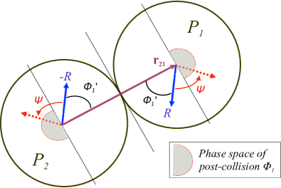
Figure 2: Configuration of 2 particle collision in 2 dimensions in the center-of-mass frame

Given the pre-collision angle $\phi_{1}^{{}^{\prime}}$, the problem at hand is the generation of a reversible random offset $\psi$ from $\phi_{1}^{{}^{\prime}}$ to give the post-collision angle $\phi_{1}=\phi_{1}^{{}^{\prime}}+\psi$ which can then be used to determine the post-collision velocities. Since the phase space of $\phi_{1}$ is $[0,2\pi)$, it is necessary to sample the random offset $\psi$ also from the same range, in order to ensure full phase space coverage independent of $\phi_{1}^{{}^{\prime}}$. This is illustrated in Figure 2 in which the colliding pair is visualized in its center-of-mass frame of reference (in this particular case of 2-particles in 2-dimensions, the geometric angle $\phi_{1}$ indeed corresponds to the degree of freedom, but this does is not true in general). Moreover since the circumference of the circle is uniformly sampled by uniformly sampling the angle subtended at the center, it is sufficient to generate $\psi$ uniformly from 0 to $2\pi$. Thus, $\psi\in[0,2\pi)$ is generated with a ${\bm{G}}$-to-${\bm{\Psi}}$ mapping given by $\psi=2G\pi$, with a uniformly distributed random number $G\in[0,1)$.

However, the $\phi_{1}$ value thus computed may violate the geometry constraint Equation (8) on post-collision velocities. If such a violation occurs with the generated random offset, the $\phi_{1}$ value can be “corrected” by adding $\pi$ to it; the addition of $\pi$ guarantees satisfaction of the geometry constraint on post-collision velocities because of the following observations:

Since $$(a-b)=2R\cos\phi_{1}\text{, and }(c-d)=2R\sin\phi_{1},$$ (11)

if $$r_{21x}\cdot(a-b)+r_{21y}\cdot(c-d) <0$$

then $$r_{21x}\cdot(2R\cos\phi_{1})+r_{21y}\cdot(2R\sin\phi_{1}) <0$$

$$\implies r_{21x}\cdot(2R\cos(\phi_{1}+\pi))+r_{21y}\cdot(2R\sin(\phi_{1}+\pi)) >0.$$

Thus, the post-collision angle, using the random angle offset $\psi$, is computed as either ${\bm{F}:}~{}\phi_{1}=\phi_{1}^{{}^{\prime}}+\psi$ or ${\bm{F}_{\pi}:}~{}\phi_{1}=\phi_{1}^{{}^{\prime}}+\psi+\pi$. In reverse execution, the pre-collision angle $\phi_{1}^{{}^{\prime}}$ is recovered as ${\bm{R}:}~{}\phi_{1}^{{}^{\prime}}=\phi_{1}-\psi$ or ${\bm{R}_{\pi}:}~{}\phi_{1}^{{}^{\prime}}=\phi_{1}-\psi-\pi$. If the fact that $\pi$ was added by the forward execution is somehow remembered (i.e., whether ${\bm{F}}$ or ${\bm{F}_{\pi}}$ was applied), then the correct pre-collision angle can be recovered during reversal (by applying ${\bm{R}}$ or ${\bm{R}_{\pi}}$ respectively).

Our key observation here is that it is possible to avoid having to “remember” whether the $\pi$ offset was added or not. If $\pi$ was added in forward execution, then, in reverse execution, the fact that $\psi+\pi$ must be used, as opposed to $\psi$, can be detected by a violation of the geometry constraint on the pre-collision velocities if $\pi$ is not added. The correct value of $\phi_{1}^{{}^{\prime}}=\phi_{1}-\psi-\pi$ is thus possible to be recovered correctly.

To adopt this approach, it is necessary and sufficient to show that no ambiguity exists during the reverse execution regarding which of ${\bm{F}}$ or ${\bm{F}_{\pi}}$ was executed in the forward execution, so that the correct operation, ${\bm{R}}$ or ${\bm{R}_{\pi}}$, is applied for correct reversal. In other words, it is necessary and sufficient to satisfy the following conditions:
$\bullet$ ${\bm{R}}({\bm{F}}(\phi))=\phi$ $\bullet$ ${\bm{R}_{\pi}}({\bm{F}}(\phi))\neq\phi$ $\bullet$ ${\bm{R}_{\pi}}({\bm{F}_{\pi}}(\phi))=\phi$ $\bullet$ ${\bm{R}}({\bm{F}_{\pi}}(\phi))\neq\phi$ $\bullet$ ${\bm{F}}(\phi)\neq{\bm{F}_{\pi}}(\phi))$ $\bullet$ ${\bm{R}}(\phi)\neq{\bm{R}_{\pi}}(\phi))$.

These conditions can be proven as follows. Let $CS(\phi)=r_{21x}\cdot(2R\cos\phi)+r_{21y}\cdot(2R\sin\phi)$. We know that ${\bm{F}}$ and ${\bm{F}_{\pi}}$ are exclusive with respect to satisfaction of Equation (8) with $\phi_{1}$, i.e., ${\bm{F}}$ satisfies $CS(\phi_{1})>0$, if and only if ${\bm{F}_{\pi}}$ satisfies $CS(\phi_{1})<0$. Similarly, ${\bm{R}}$ and ${\bm{R}_{\pi}}$ are exclusive with respect to satisfaction of Equation (8) with $\phi_{1}^{{}^{\prime}}$, i.e., ${\bm{R}}$ satisfies $CS(\phi_{1}^{{}^{\prime}})<0$, if and only if ${\bm{R}_{\pi}}$ satisfies $CS(\phi_{1}^{{}^{\prime}})>0$.

The geometrical constraints require that the post-collision velocities satisfy $CS(\phi_{1})>0$ and the pre-collision velocities satisfy $CS(\phi_{1}^{{}^{\prime}})<0$. These requirements are satisfied if ${\bm{R}}$ is used to reverse ${\bm{F}}$, or ${\bm{R}_{\pi}}$ is used to reverse ${\bm{F}_{\pi}}$, respectively. In other words, from Equation (11), we know that:
$\bullet$ if ${\bm{F}}$ satisfies $CS(\phi_{1})>0$ in forward, then ${\bm{R}}$ satisfies $CS(\phi_{1}^{{}^{\prime}})<0$ in reverse, and
$\bullet$ if ${\bm{F}_{\pi}}$ satisfies $CS(\phi_{1})>0$ in forward, then ${\bm{R}_{\pi}}$ satisfies $CS(\phi_{1}^{{}^{\prime}})<0$ in reverse.

Finally, the ambiguity is fully resolved when the following are also satisfied:
$\bullet$ If ${\bm{F}}$ satisfies $CS(\phi_{1})>0$, then ${\bm{R}_{\pi}}$ violates $CS(\phi_{1}^{{}^{\prime}})<0$.
$\bullet$ If ${\bm{F}_{\pi}}$ satisfies $CS(\phi_{1})>0$, then ${\bm{R}}$ violates $CS(\phi_{1}^{{}^{\prime}})<0$.

The former can be proved as follows, and the latter can be proved along similar lines: Since $CS(\phi_{1}^{{}^{\prime}})<0$ (pre-collision), and ${\bm{F}}$ gives $CS(\phi_{1})>0$ (post-collision), ${\bm{R}_{\pi}}$ gives $CS(\phi_{1}-\psi-\pi)$ $=CS(\overline{\phi_{1}^{{}^{\prime}}+\psi}-\psi-\pi)$ $=CS(\phi_{1}^{{}^{\prime}}-\pi)$ $=-CS(\phi_{1}^{{}^{\prime}})$. This implies $CS(\phi_{1}^{{}^{\prime}})=-CS(\phi_{1}^{{}^{\prime}})$, which is a contradiction.

The forward and reverse algorithms are given in Procedure 1 and Procedure 2 respectively. This completes the generation of reversible random offsets for all configurations of 2-particle collisions in 2 dimensions, ensuring full phase space coverage with zero memory overhead.

Procedure 1 ($\phi_{1}^{{}^{\prime}}\longrightarrow\phi_{1}$): Forward Function for 2-Particle in 2 Dimensions

1:  $\psi\leftarrow 2G\pi$ {generate a random offset from $[0,2\pi)$}

2:  $\phi_{1}\leftarrow(\phi_{1}^{{}^{\prime}}+\psi)\mod 2\pi$ {post-collision is pre-collision offset by randomized $\psi$}

3:  {Next, if post-collision is converging, correct it to be diverging}

4:  if $r_{21x}\cdot\cos{\phi_{1}}+r_{21y}\cdot\sin{\phi_{1}}<0$ then

5:     $\phi_{1}\leftarrow(\phi_{1}+\pi)\mod 2\pi$

6:  end if

Procedure 2 ($\phi_{1}\longrightarrow\phi_{1}^{{}^{\prime}}$): Reverse Function for 2-Particle in 2 Dimensions

1:  $\psi\leftarrow 2G\pi$ {recover the random offset}

2:  $\phi_{1}^{{}^{\prime}}\leftarrow(\phi_{1}-\psi)\mod 2\pi$ {initial guess at pre-collision angle}

3:  {Next, if pre-collision is diverging, correct it to be converging}

4:  if $r_{21x}\cdot\cos{\phi_{1}}+r_{21y}\cdot\sin{\phi_{1}}>0$ then

5:     $\phi_{1}^{{}^{\prime}}\leftarrow(\phi_{1}^{{}^{\prime}}-\pi)\mod 2\pi$

6:  end if

4.3 Reversal for 2-Particle Collisions in 3 Dimensions

In a collision of 2 particles in 3-dimensional space, the equations of motion and post-collision geometry are:

$$\left.\begin{aligned} a+b=\alpha\text{, }c+d=\beta\text{, }e+f=\gamma\\ a^{2}+b^{2}+c^{2}+d^{2}+e^{2}+f^{2}=\delta\text{, and }2\delta>\alpha^{2}+\beta^{2}+\gamma^{2}\end{aligned}\right\}\text{Dynamics},$$ (12)

$$\left.\begin{aligned} r_{21x}\cdot(a-b)+r_{21y}\cdot(c-d)+r_{21z}\cdot(e-f)&>0\\ \text{for some }r_{21x},r_{21y},r_{21z}&>0&\end{aligned}\right\}\text{Geometry}.$$ (13)

The pre-collision geometrical constraints are obtained by replacing $>0$ by $<0$ in the post-collision constraints. The equations of motion imply that:

$$\left(a-\frac{\alpha}{2}\right)^{2}+\left(c-\frac{\beta}{2}\right)^{2}+\left(e-\frac{\gamma}{2}\right)^{2}=\frac{2\delta-(\alpha^{2}+\beta^{2}+\gamma^{2})}{4}=R^{2},$$ (14)

i.e., the point ($a$, $c$, $e$) lies on a sphere of radius $R=\tfrac{1}{2}\sqrt{2\delta-(\alpha^{2}+\beta^{2}+\gamma^{2})}$ centered at ($\tfrac{\alpha}{2}$, $\tfrac{\beta}{2}$, $\tfrac{\gamma}{2}$). whose parametric equations are given by:

$$a=\frac{\alpha}{2}+R\sin{\phi_{1}}\sin{\phi_{2}}\text{, }c=\frac{\beta}{2}+R\sin{\phi_{1}}\cos{\phi_{2}}\text{, }e=\frac{\gamma}{2}+R\cos{\phi_{1}}\text{,}$$ (15)

$$\phi_{1}\in[0,\pi]\text{, and }\phi_{2}\in[0,2\pi)~{}.$$

Equation (15) provides the ${\bm{V}}$-to-${\bm{\Phi}}$ and ${\bm{\Phi}}$-to-${\bm{V}}$ mapping functions for 2-particle collisions in 3 dimensions.

In determining ${\bm{\Phi}}$ from ${\bm{V}}$, if $\phi_{1}=0$ or $\phi_{1}=\pi$, then, the value of $\phi_{2}$ is immaterial. In that case, we choose to set $\phi_{2}=0$. Setting $\phi_{2}$ thus, without regard to $\phi_{2}^{{}^{\prime}}$, loses information about $\phi_{2}^{{}^{\prime}}$ when $\phi_{1}=0$. To deal with this rare special case, the value of $\phi_{2}^{{}^{\prime}}$ can be logged in the forward collision, and restored from the log in the backward collision. Note that this is logged in forward execution only if $\phi_{1}=0$, and not for every collision. In the reverse execution, $\phi_{2}^{{}^{\prime}}$ is recovered from the log only if $\phi_{1}=0$.

For the ${\bm{G}}$-to-${\bm{\Psi}}$ mapping, the offsets $\psi_{1}$ and $\psi_{2}$ are obtained by uniformly sampling the surface of a unit sphere. Any algorithm for this purpose can be employed (e.g., [Mar72]), using two random numbers $G_{1}\in[0,1]$ and $G_{2}\in[0,1)$.

Similar to the 2-dimensional 2-particle case, the post-collision angles are computed as $\phi_{1}=(\phi_{1}^{{}^{\prime}}+\psi_{1})\mod 2\pi$ or $\phi_{1}=(\phi_{1}^{{}^{\prime}}+\psi_{1}+\pi)\mod 2\pi$, and $\phi_{2}=(\phi_{2}^{{}^{\prime}}+\psi_{2})\mod 2\pi$. The choice of whether $\pi$ is added to $\psi$ is determined by the one that satisfies the geometrical condition given by Equation (13). The proof of reversibility of the computation of $\phi_{1}$ is analogous to the one in the preceding sub-section.

This completes the generation of reversible random offsets for all configurations of 2-particle collisions in three dimensions, ensuring full phase space coverage with zero memory overhead.

4.4 Reversal for 3-Particle Collisions in 1 Dimension

In this section, we determine the phase space of the permissible reversible random offsets that needs to be sampled for 3-particle collisions in 1 dimension.

4.4.1 Solving the Equations of Motion

The equations of motion are:

$$\left.\begin{aligned} a+b+c&=\alpha\\ a^{2}+b^{2}+c^{2}&=\delta\text{, }3\delta&>\alpha^{2}\end{aligned}\right\}\text{Dynamics}.$$ (16)

The post-collision geometrical constraints are given by:

$$\left[\begin{aligned} \text{Only two of these three need be}\\ \text{satisfied for any given geometric}\\ \text{configuration }r_{21},r_{32},r_{13}>0\end{aligned}\right]\left.\begin{aligned} r_{21}\cdot(a-b)&>0,\\ r_{32}\cdot(b-c)&>0,\\ r_{13}\cdot(c-a)&>0\end{aligned}\right\}\text{Geometry}.$$ (17)

In Equation (17), when any two inequalities are satisfied, the third one is resulting. This is because the two inequalities that are satisfied imply a specific ordering of the three particles along the single dimension, which in turn automatically satisfies the remaining third constraint. The pre-collision geometrical constraints are obtained by replacing $>0$ by $<0$ in the post-collision constraints. The solution to the equations of motion satisfies:

$$\bar{a}^{2}+{\left(\frac{\bar{b}-\frac{\sqrt{2}}{3}\alpha}{\dfrac{1}{\sqrt{3}}}\right)}^{2} =\delta-\frac{\alpha^{2}}{3}\text{, where }\bar{a} =\frac{a-b}{\sqrt{2}}\text{, and }\bar{b} =\frac{a+b}{\sqrt{2}},$$ (18)

which leads to the parametrization:

$$\bar{a} =\frac{\lambda}{\sqrt{2}}\cos{\phi_{1}}\text{, }\bar{b} =\frac{\sqrt{2}}{3}\alpha+\frac{\lambda}{\sqrt{2}\sqrt{3}}\sin{\phi_{1}}\text{, }\lambda =\sqrt{2}\sqrt{\delta-\frac{\alpha^{2}}{3}}\text{, and }\phi_{1} \in[0,2\pi).$$ (19)

Converting to $a$, $b$ and $c$, we get:

$$\begin{aligned} a=\frac{\alpha}{3}+\frac{\lambda}{2}(\cos{\phi_{1}}+\frac{1}{\sqrt{3}}\sin{\phi_{1}})\text{, }b=\frac{\alpha}{3}+\frac{\lambda}{2}(-\cos{\phi_{1}}+\frac{1}{\sqrt{3}}\sin{\phi_{1}})\text{,}\\ c=\frac{\alpha}{3}+\frac{\lambda}{2}(-\frac{2}{\sqrt{3}}\sin{\phi_{1}})\text{, }\lambda=\sqrt{2}\sqrt{\delta-\frac{\alpha^{2}}{3}}\text{, and }\phi_{1}\in[0,2\pi).\end{aligned}$$ (20)

Equation (20) provides the ${\bm{V}}$-to-${\bm{\Phi}}$ and ${\bm{\Phi}}$-to-${\bm{V}}$ mapping functions for 1-dimensional 3-particle collisions.

4.4.2 Sampling the ${\bm{\Psi}}$ Phase Space

Analogously to the 2-particle 2-dimensional case, the phase space of the post-collision angle is sampled by generating a random $\phi_{1}$ as a random offset $\psi_{1}\in[0,2\pi)$ from the pre-collision angle $\phi_{1}^{{}^{\prime}}$. The mapping function from a uniform random number $G\in[0,1)$ to $\psi_{1}$ is more complex than that for the 2-particle case. In the 2-particle case, the phase space for velocities lies on the circumference of a circle, which can be sampled simply by uniformly sampling the angle subtended at the center. However, the phase space of the velocities in the 3-particle case lies on the circumference of an ellipse, which cannot be sampled simply as $\psi_{1}=2G\pi$. Instead, any correctly unbiased procedure for generating the angle by sampling the circumference of an ellipse can be employed for the purpose of defining the ${\bm{G}}$-to-${\bm{\Psi}}$ mapping function. One such method is described in the next section.

4.4.3 Sampling the Circumference of the Ellipse

Here, we present a new procedure for uniformly sampling a point from the perimeter of an ellipse. The procedure is designed to be suitable for use in reversible execution, requiring exactly one random number per sample. While rejection-based procedures exist for this problem, they cannot be used here due to their irreversibility, as explained later in Section 4.6.

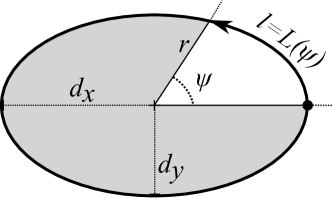
Figure 3: Sampling scheme for a uniformly selected random point on an ellipse

Consider the ellipse $\left(\tfrac{x}{d_{x}}\right)^{2}+\left(\tfrac{y}{d_{y}}\right)^{2}=1$ shown in Figure 3. Let $L:\psi\rightarrow\ell$ be a function that maps any angle $\psi$, $0\leq\psi<2\pi$, to the length $\ell$ of the arc moving counter-clockwise along the circumference of the ellipse from $(d_{x},0)$ to $(r\cos{\psi},r\sin{\psi})$, where $r^{2}={d_{x}^{2}d_{y}^{2}}/({d_{y}^{2}\cos{\psi}^{2}+d_{x}^{2}\sin{\psi}^{2}})$. Let $L^{-1}:\ell\rightarrow\psi$ be the inverse function that determines the angle corresponding to any given arc length $\ell$. Thus, $L^{-1}(L(\psi))=\psi$. A random point on the circumference of the ellipse can be obtained as the end of the arc whose length is $G\cdot L(2\pi)$, and the angle corresponding to that point can be obtained as $\psi_{1}=L^{-1}(G\cdot L(2\pi))$, which serves as the ${\bm{G}}$-to-${\bm{\Psi}}$ mapping for the 3-particle collisions in 1 dimension.

The value of $L(2\pi)$ is computable by different methods. For example, $L(2\pi)=\pi(d_{x}+d_{y})\sum_{n=0}^{\infty}{\binom{0.5}{n}^{2}h^{n}}$, where $h=\tfrac{(d_{x}-d_{y})^{2}}{(d_{x}+d_{y})^{2}}$, which can be computed to any desired precision. The value of $L^{-1}(\ell_{given})$ can be obtained by a bisection method (binary search) that starts with the lowerbound $\psi_{lower}=0$ upperbound $\psi_{upper}=2\pi$, and an initial estimate value of $\psi_{guess}=\pi$, and repeatedly adjusts the lowerbound or upperbound to the guess value (depending on whether $L(\psi_{guess})<\ell_{given}$ or $\ell_{given}<L(\psi_{guess})$ respectively), until the correct angle corresponding to $\ell_{given}$ is determined.

For the ellipse in Equation (18), $d_{x}=\sqrt{\delta-\tfrac{\alpha^{2}}{3}}$ and $d_{y}=\tfrac{d_{x}}{\sqrt{3}}$. Since $d_{x}$ and $d_{y}$ only depend on $\delta$ and $\alpha$, the value of $\psi_{1}$ can be generated and recovered (re-generated) independently of individual particle velocities.

Note that the computational burden in sampling the ellipse occurs both in log-based approaches and in our approach. Thus, the forward portions incur the same computational cost. However, we use the same computational procedure on the reverse path, to re-generate the sample and use it in the reverse procedure. Since log-based approaches rely on memory, they do not incur computational cost on the reverse path, but incur extra memory copying cost in forward execution. In a normal, well-balanced parallel execution, since reversals of collisions are far fewer than forward collisions, the extra computational cost of our approach in the reverse procedure is much less than the savings gained in foward execution compared to log-based approaches, resulting in an overall reduction in run time and memory.

4.4.4 Resolving the Geometrical Constraints

Note that, with the sampled $\phi_{1}=\phi_{1}^{{}^{\prime}}+\psi$, it is possible to correctly recover the pre-collision angle $\phi_{1}^{{}^{\prime}}$, from which the values of the pre-collision velocities can be recovered, but not necessarily their correct assignation to the identities of the particles. Thus, there still remains the problem of uniquely recovering the configuration of the particles, since the preceding solution provides for two different but equivalent configurations that only differ in that their left and right particle identities are swapped. Without modifying the procedure, one additional bit of memory would be needed for each collision to disambiguate between the two configurations. Since the aim is to completely eliminate memory accumulation, the model needs additional development for reversibility, as presented next.

Equation (20) gives the key terms in the geometrical constraints as:

$$\begin{aligned} (a-b)&=\lambda\cos{\phi_{1}}\text{, }(b-c)&=\lambda\cos{(\phi_{1}-\frac{2\pi}{3})}\text{, and }(c-a)&=\lambda\cos{(\phi_{1}+\frac{2\pi}{3})}.\end{aligned}$$ (21)

Equation (21) indicates the permissible phase space of $\phi_{1}$ with the property that we exploit here for reversibility, namely, that the three terms $\cos\phi$, $\cos(\phi-\tfrac{2\pi}{3})$, and $\cos(\phi+\tfrac{2\pi}{3})$ never carry the same sign, i.e., if one is negative, the other two are non-negative, and if one is positive, the other two are non-positive (see Figure 4).

From Equation (21), we deduce:

$$\begin{aligned} \cos{\phi_{1}}+\cos{(\phi_{1}-\frac{2\pi}{3})}+\cos{(\phi_{1}+\frac{2\pi}{3})}=0\text{, since }\lambda>0.\end{aligned}$$ (22)

Figure 4: Variation of the geometrical terms with $\phi_{1}$ in 3-particle collisions in 1 dimension

Without loss of generality, let $a^{{}^{\prime}}$, $b^{{}^{\prime}}$, and $c^{{}^{\prime}}$ represent the pre-collision velocities of the left, center and right particles, respectively, colliding along the one-dimensional path. This is illustrated in Figure 5. Let the corresponding post-collision velocities be $a$, $b$, and $c$, respectively. Define a canonical assignation of $\phi_{1}^{{}^{\prime}}$ such that $a^{{}^{\prime}}-b^{{}^{\prime}}=R\cos{\phi_{1}^{{}^{\prime}}}$, $b^{{}^{\prime}}-c^{{}^{\prime}}=R\cos{(\phi_{1}^{{}^{\prime}}-\tfrac{2\pi}{3})}$, and $c^{{}^{\prime}}-a^{{}^{\prime}}=R\cos{(\phi_{1}^{{}^{\prime}}+\tfrac{2\pi}{3})}$. Note that this convention fully covers the phase space of all pre-collision velocities for the given total momentum and kinetic energy, and in that sense, is general and equivalent to any other valid convention.

Figure 5: Canonical configuration of 3 particles in 1 dimension

Pre-collision: For the left and center particles to collide, $a^{{}^{\prime}}-b^{{}^{\prime}}>0$. Similarly, for the center and right particles to collide, $b^{{}^{\prime}}-c^{{}^{\prime}}>0$. These two conditions constrain the range of $\phi_{1}^{{}^{\prime}}$ to $[\tfrac{\pi}{6},\tfrac{\pi}{2})$, since it is only for that range of $\phi_{1}^{{}^{\prime}}$ that $\cos{\phi_{1}^{{}^{\prime}}}$ and $\cos{(\phi_{1}^{{}^{\prime}}-\tfrac{2\pi}{3})}$ are both non-negative. The exact value of $\phi_{1}^{{}^{\prime}}$ in that range is determined from the following:

$$\begin{aligned} \bar{a}^{{}^{\prime}}=\frac{a^{{}^{\prime}}-b^{{}^{\prime}}}{\sqrt{2}}\text{, }\bar{b}^{{}^{\prime}}=\frac{a^{{}^{\prime}}+b^{{}^{\prime}}}{\sqrt{2}}\text{, and }\tan{\phi_{1}^{{}^{\prime}}}=\frac{\sqrt{3}\left(\bar{b}^{{}^{\prime}}-\frac{\sqrt{2}}{3}\alpha\right)}{\bar{a}^{{}^{\prime}}}\text{.}\end{aligned}$$ (23)

Thus, any pre-collision configuration of ($a^{{}^{\prime}}$, $b^{{}^{\prime}}$, $c^{{}^{\prime}}$) velocities of left, center, and right particles can be uniquely and completely represented by ($\phi_{1}^{{}^{\prime}}$, $\alpha$, $\delta$), where $\tfrac{\pi}{6}\leq\phi_{1}^{{}^{\prime}}<\tfrac{\pi}{2}$.

Post-collision: For the left and center particles to diverge after collision (i.e., not to pass through each other), their post-collision velocities must satisfy $a-b<0$. Similarly, for the center and right particles, $b-c<0$. These two conditions constrain the range of $\phi_{1}$ to $[\tfrac{7\pi}{6},\tfrac{3\pi}{2})$, which is essentially offset by $+\pi$ from the range of $\phi_{1}^{{}^{\prime}}$.

Pictorially, the regions of interest in the $[0,2\pi)$ range are given in Figure 6. The full $[0,2\pi)$ range is divided into six regions, each spanning $\tfrac{2\pi}{3}$. The first region starts at $\tfrac{\pi}{6}$. In the figure, $R1$ is the range of $\phi_{1}^{{}^{\prime}}$ (pre-collision), and $S1$ is the range of $\phi_{1}$ (post-collision). Any given angle $\phi_{1}^{{}^{\prime}}$ in $R1$ corresponds to a set of three velocities $\{a^{{}^{\prime}},b^{{}^{\prime}},c^{{}^{\prime}}\}$, such that the pre-collision geometrical constraints of Equation (17) are satisfied, implying a specifically ordered sequence of the particles, say, $a;b;c$, along one dimension. The regions $R2$ and $R3$ correspond to left-rotation of the $R1$ sequence, namely, $c;a;b$ and $b;c;a$, obtained by offsetting $\phi_{1}^{{}^{\prime}}$ by $+\tfrac{2\pi}{3}$ and $-\tfrac{2\pi}{3}$, respectively. Similarly, the regions $S2$ and $S3$ correspond to the right-rotation of the $S1$ sequence. Note that the pre-collision and post-collision angles only fall in the $R1$ and $S1$ regions, respectively, and the other regions are unreachable by the system. They are defined and used in intermediate calculations when computing post-collision angles in forward execution (and recovering pre-collision angles in reverse) while ensuring full phase space coverage.

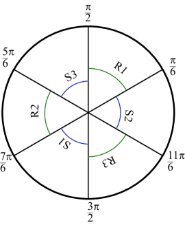
Figure 6: Division of the angular space for $\phi_{1}$ and $\phi_{1}^{{}^{\prime}}$ in 3-particle collisions in 1 dimension

Reversible Sampling: The problem of making the collision reversible now becomes equivalent to defining a reversible (i.e., one-to-one and onto) mapping from any given $\phi_{1}^{{}^{\prime}}\in[\tfrac{\pi}{6},\tfrac{\pi}{2})$ to a random sample of $\phi_{1}\in[\tfrac{7\pi}{6},\tfrac{3\pi}{2})$, while accurately preserving the underlying distribution of velocities along the circumference of the ellipse in Equation (18). In general, any such bijection could serve the purpose. Here, such a mapping function is provided in Procedure 3 (forward) and Procedure 4 (reverse).

The forward function essentially rotates $\phi_{1}^{{}^{\prime}}$ uniformly over the entire range $[0,2\pi)$ first, and then makes adjustments reversibly, as needed, to map back to the valid range $[\tfrac{7\pi}{6},\tfrac{3\pi}{2})$ of $\phi_{1}$.

Procedure 3 ($\phi_{1}^{{}^{\prime}}\longrightarrow\phi_{1}$): Forward Function for 3-Particle in 1 Dimension

  $\ell\leftarrow G\cdot L(2\pi)$ {Pick a random arc length on ellipse}

  $\psi_{1}\leftarrow L^{-1}(\ell)$ {Find angle corresponding to arc length}

  {Compute post-collision angle}

  $\phi_{1}\leftarrow(\phi_{1}^{{}^{\prime}}+\psi_{1})\mod 2\pi$ {Step 1}

  {Adjust post-collision angle if/as necessary}

  if more than one of $\cos{\phi_{1}}$, $\cos{(\phi_{1}-\tfrac{2\pi}{3})}$ and $\cos{(\phi_{1}+\tfrac{2\pi}{3})}$ is positive then

     $\phi_{1}\leftarrow(\phi_{1}+\pi)\mod 2\pi$ {Step 2}

  end if

  if $\cos{\phi_{1}}$ is positive then

     $\phi_{1}\leftarrow(\phi_{1}-\tfrac{2\pi}{3})\mod 2\pi$ {Step 3a}

  else if $\cos{(\phi_{1}-\tfrac{2\pi}{3})}$ is positive then

     $\phi_{1}\leftarrow(\phi_{1}+\tfrac{2\pi}{3})\mod 2\pi$ {Step 3b}

  end if

The operation of Procedure 3 is illustrated in Equation (24). Step 1 adds a random offset in $[0,2\pi)$ to $\phi_{1}^{{}^{\prime}}$ to get a candidate sample of $\phi_{1}$. Clearly, the candidate may fall in any of the six regions shown in Figure 6. The first correction is to detect if the candidate angle maps to R1, R2, or R3, and if so, remap it to S1, S2, or S3 respectively (because post-collision velocities must diverge, which implies that the post-collision free angle cannot be in R1, R2, or R3). This is accomplished in Step 2 by adding $\pi$ to the candidate. In Step 3, if the candidate happens to already be in S1, then no additional adjustments are needed. Otherwise, if it falls in S3, it is wrapped back to S1 by rotating it counter-clockwise by $\tfrac{2\pi}{3}$ (Step 3a), and if it falls in S2, it is wrapped back to S1 by rotating it clockwise by $\tfrac{2\pi}{3}$ (Step 3b). To summarize:

$$\phi_{1}^{{}^{\prime}}\in\left\{R1\right\}\xrightarrow[\text{randomize}]{\text{Step 1}}\phi_{1}\in\left\{S1,S2,S3,R1,R2,R3\right\}\xrightarrow[\text{maps to}]{\text{Step 2}}\cdots$$

$$\cdots\xrightarrow[\text{maps to}]{\text{Step 2}}\phi_{1}\in\left\{S1,S2,S3\right\}\xrightarrow[\text{maps to}]{\text{Step 3}}\phi_{1}\in\left\{S1\right\}\text{ .}$$ (24)

The reverse function shown in Procedure 4 uncovers the random offset first, and reconstructs a candidate $\phi_{1}^{{}^{\prime}}$. It detects adjustments, if any, that were made during forward execution, and then performs the opposite of adjustments to recover the correct original value of $\phi_{1}^{{}^{\prime}}$.

Procedure 4 ($\phi_{1}\longrightarrow\phi_{1}^{{}^{\prime}}$): Reverse Function for 3-Particle in 1 Dimension

  $\ell\leftarrow G\cdot L(2\pi)$ {Recover the random arc length on ellipse}

  $\psi_{1}\leftarrow L^{-1}(\ell)$ {Recover the angle corresponding to arc length}

  {Compute initial guess of pre-collision angle}

  $\phi_{1}^{{}^{\prime}}\leftarrow(\phi_{1}-\psi_{1})\mod 2\pi$

  {Correct the guess if/as necessary} {Step 1}

  if more than one of $\cos{\phi_{1}}$, $\cos{(\phi_{1}-\tfrac{2\pi}{3})}$ and $\cos{(\phi_{1}+\tfrac{2\pi}{3})}$ is positive then

     $\phi_{1}^{{}^{\prime}}\leftarrow(\phi_{1}^{{}^{\prime}}-\pi)\mod 2\pi$ {Step 2}

  end if

  if $\cos{\phi_{1}^{{}^{\prime}}}$ is negative then

     $\phi_{1}^{{}^{\prime}}\leftarrow(\phi_{1}^{{}^{\prime}}-\tfrac{2\pi}{3})\mod 2\pi$ {Step 3a}

  else if $\cos{(\phi_{1}^{{}^{\prime}}-\tfrac{2\pi}{3})}$ is negative then

     $\phi_{1}^{{}^{\prime}}\leftarrow(\phi_{1}^{{}^{\prime}}+\tfrac{2\pi}{3})\mod 2\pi$ {Step 3b}

  end if

The operation of Procedure 4 is illustrated in Equation (25). Step 1 removes the random offset in $[0,2\pi)$ from $\phi_{1}$ to get a first guess of the original $\phi_{1}^{{}^{\prime}}$. Clearly, the guessed value may fall in any of the six regions shown in Figure 6. The first correction to the guess is to detect if the candidate angle maps to S1, S2, or S3, and if so, remap it to R1, R2, or R3 respectively (because pre-collision velocities must be converging, which implies that the pre-collision free angle cannot be in S1, S2, or S3). This is accomplished in Step 2 by subtracting $\pi$ from the guessed value. In Step 3, if the guess happens to already be in R1, then it already represent the correct original value of $\phi_{1}^{{}^{\prime}}$. Otherwise, if it falls in R2, it is wrapped back to R1 by rotating it clockwise by $\tfrac{2\pi}{3}$ (Step 3a), and if it falls in R3, it is wrapped forward to R1 by rotating it counter-clockwise by $\tfrac{2\pi}{3}$ (Step 3b). To summarize:

$$\phi_{1}^{{}^{\prime}}\in\left\{R1\right\}\xleftarrow[\text{maps to}]{\text{Step 3}}\phi_{1}^{{}^{\prime}}\in\left\{R1,R2,R3\right\}\xleftarrow[\text{maps to}]{\text{Step 2}}\cdots$$

$$\cdots\xleftarrow[\text{maps to}]{\text{Step 2}}\phi_{1}^{{}^{\prime}}\in\left\{S1,S2,S3,R1,R2,R3\right\}\xleftarrow[\text{de-randomize}]{\text{Step 1}}\phi_{1}\in\left\{S1\right\}\text{ .}$$ (25)

4.4.5 Combining Dynamics and Geometry

The series of transformations performed in forward and reverse collision operations is summarized in Equation (26), which shows the input of the three pre-collision velocities $(a^{\prime},b^{\prime},c^{\prime})$ being transformed by the ${\bm{V}}$-to-${\bm{\Phi}}$ mapping into the triple formed by the angle $\phi_{1}^{{}^{\prime}}$, momentum $\alpha$, and energy $\delta$. These are fed into the forward parts of the Function 1 or Function 2 with an additional input, which is the uniformly distributed random number $G$. The resulting triple of the post-collision angle $\phi_{1}$ together with momentum and energy are transformed by the ${\bm{\Phi}}$-to-${\bm{V}}$ mapping into the post-collision velocities $(a,b,c)$. For reversal, the forward process is inverted by first recovering the angle $\phi_{1}$ upon applying the ${\bm{V}}$-to-${\bm{\Phi}}$ mapping on the post-collision velocities. The random number $G$ is recovered by retracing the random number sequence, and the reverse part of the function is applied to recover $\phi_{1}^{{}^{\prime}}$, from which the pre-collision velocities are obtained by applying the ${\bm{\Phi}}$-to-${\bm{V}}$ mapping on the recovered angle.

$$\begin{aligned} (a^{{}^{\prime}},b^{{}^{\prime}},c^{{}^{\prime}})&\xrightarrow{\textbf{${\bm{V}}$-to-${\bm{\Phi}}$}}&(\phi_{1}^{{}^{\prime}},\alpha,\delta)&\xrightarrow{\text{Forward}}&(\phi_{1},\alpha,\delta)&\xrightarrow{\textbf{${\bm{\Phi}}$-to-${\bm{V}}$}}&(a,b,c)\\ &&&\quad\begin{array}[]{c}\mathrel{\raisebox{1.00006pt}{\reflectbox{\rotatebox[origin={c}]{90.0}{$\leadsto$}}}}\\ \text{G}\\ \mathrel{\raisebox{1.00006pt}{\reflectbox{\rotatebox[origin={c}]{270.0}{$\leadsto$}}}}\end{array}&&&{\Big{\downarrow}}\\ (a^{{}^{\prime}},b^{{}^{\prime}},c^{{}^{\prime}})&\xleftarrow{\textbf{${\bm{\Phi}}$-to-${\bm{V}}$}}&(\phi_{1}^{{}^{\prime}},\alpha,\delta)&\xleftarrow{\text{Reverse}}&(\phi_{1},\alpha,\delta)&\xleftarrow{\textbf{${\bm{V}}$-to-${\bm{\Phi}}$}}&(a,b,c)\end{aligned}$$ (26)

4.5 Reversal for 3-Particle Collisions in 2 Dimensions

In a collision of three particles in 2-dimensional space, the equations of motion are:

$$\left.\begin{aligned} a+b+c&=\alpha\\ d+e+f&=\beta\\ a^{2}+b^{2}+c^{2}+d^{2}+e^{2}+f^{2}&=\delta\\ 3\delta&>\alpha^{2}+\beta^{2}\end{aligned}\right\}\text{Dynamics}.$$ (27)

The geometrical constraints satisfied by the post-collision velocities are:

$$\left.\begin{aligned} r_{21x}\cdot(a-b)+r_{21y}\cdot(d-e)&>0,&\text{if {P1} and {P2} are in contact}\\ r_{32x}\cdot(b-c)+r_{32y}\cdot(e-f)&>0,&\text{if {P2} and {P3} are in contact}\\ r_{13x}\cdot(c-a)+r_{13y}\cdot(f-d)&>0&\text{if {P3} and {P1} are in contact}\\ \end{aligned}\right\}\text{Geometry}.$$ (28)

The pre-collision geometrical constraints are obtained by replacing $>0$ by $<0$ in the post-collision constraints. In Equation (28), we will use K1 to denote the first inequality (P1 and P2 in contact), K2 to denote the second inequality, and K3 to denote the third.

The solution to the equations of motion satisfies the hyper-ellipsoid equation:

$${\left(\frac{\bar{a}-0}{1}\right)}^{2}+{\left(\frac{\bar{b}-\frac{\sqrt{2}}{3}\alpha}{\dfrac{1}{\sqrt{3}}}\right)}^{2}+{\left(\frac{\bar{d}-0}{1}\right)}^{2}+{\left(\frac{\bar{e}-\frac{\sqrt{2}}{3}\beta}{\dfrac{1}{\sqrt{3}}}\right)}^{2} =\delta-\frac{\alpha^{2}+\beta^{2}}{3}\text{,}$$ (29)

$$\text{where }\bar{a}=\frac{a-b}{\sqrt{2}}\text{, }\bar{b}=\frac{a+b}{\sqrt{2}}\text{, }\bar{d}=\frac{d-e}{\sqrt{2}}\text{, and }\bar{e}=\frac{d+e}{\sqrt{2}}~{}.$$

The hyper-ellipsoid can be described via parametic equations with three independent parameters $\left\{\phi_{1},\phi_{2},\phi_{3}\right\}$ as the degrees of freedom as follows:

$$\left.\begin{aligned} \bar{a}&=\frac{\lambda}{\sqrt{2}}\cos{\phi_{1}}\text{,}\\ \bar{d}&=\frac{\lambda}{\sqrt{2}}\sin{\phi_{1}}\cos{\phi_{2}}\text{,}\\ \bar{b}&=\frac{\sqrt{2}}{3}\alpha+\frac{\lambda}{\sqrt{2}\sqrt{3}}\sin{\phi_{1}}\sin{\phi_{2}}\cos{\phi_{3}}\text{,}\\ \bar{e}&=\frac{\sqrt{2}}{3}\beta+\frac{\lambda}{\sqrt{2}\sqrt{3}}\sin{\phi_{1}}\sin{\phi_{2}}\sin{\phi_{3}}\text{, where }\\ \lambda&=\sqrt{2}\sqrt{\delta-\frac{\alpha^{2}+\beta^{2}}{3}}\text{,}\end{aligned}\right\}\begin{aligned} \phi_{1}&\in[0,\pi]\text{, }\\ \phi_{2}&\in[0,\pi]\text{, }\\ \phi_{3}&\in[0,2\pi)\text{.}\\ \end{aligned}$$ (30)

Based on the preceding parametric equations, the terms in the geometrical constraints can be expressed as:

$$a-b =\lambda\cos{\phi_{1}}$$ (31)

$$d-e =\lambda\sin{\phi_{1}}\cos{\phi_{2}}$$

$$b-c =\frac{\lambda}{2}(\sqrt{3}\sin{\phi_{1}}\sin{\phi_{2}}\cos{\phi_{3}}-\cos{\phi_{1}})$$

$$e-f =\frac{\lambda}{2}(\sqrt{3}\sin{\phi_{1}}\sin{\phi_{2}}\sin{\phi_{3}}-\sin{\phi_{1}}\cos{\phi_{2}})$$

$$c-a =\frac{-\lambda}{2}(\sqrt{3}\sin{\phi_{1}}\sin{\phi_{2}}\cos{\phi_{3}}+\cos{\phi_{1}})$$

$$f-d =\frac{-\lambda}{2}(\sqrt{3}\sin{\phi_{1}}\sin{\phi_{2}}\sin{\phi_{3}}+\sin{\phi_{1}}\cos{\phi_{2}})~{}.$$

Note that $\sin{\phi_{1}}$ and $\sin{\phi_{2}}$ are always non-negative.

The ${\bm{V}}$-to-${\bm{\Phi}}$ and ${\bm{\Phi}}$-to-${\bm{V}}$ mappings are obtained from Equation (31) as follows:

${\bm{V}}$-to-${\bm{\Phi}}$: Given $a-f$, the angles $\phi_{1}$, $\phi_{2}$, and $\phi_{3}$ are computed as:

$$\phi_{1}= \cos^{-1}\left(\dfrac{a-b}{\lambda}\right)$$ (32)

$$\phi_{2}= \left\{\begin{aligned} 0\text{ if $\phi_{1}=0$ or $\phi_{1}=\pi$}\\ \cos^{-1}\left(\dfrac{d-e}{\lambda\sin\phi_{1}}\right)\text{ otherwise}\end{aligned}\right.$$

$$\phi_{3}= \left\{\begin{aligned} 0\text{ if $\phi_{1}=0$ or $\phi_{1}=\pi$ or $\phi_{2}=0$ or $\phi_{2}=\pi$}\\ \sin^{-1}\left(\dfrac{2(e-f)+\lambda\sin\phi_{1}\cos\phi_{2}}{\sqrt{3}\lambda\sin\phi_{1}\sin\phi_{2}}\right)\text{ otherwise}\end{aligned}\right.$$

${\bm{\Phi}}$-to-${\bm{V}}$: Given $\alpha,\beta,\delta,\phi_{1},\phi_{2},\phi_{3}$, the values of $a-f$ are computed from Equation (31).

Note that the cases of $\phi_{1}=0$ or $\phi_{1}=\pi$ or $\phi_{2}=0$ or $\phi_{2}=\pi$ are solved as follows:

$$a =\dfrac{\alpha}{3}+\dfrac{\lambda}{2}\cos\phi_{1}$$ (33)

$$b =\dfrac{\alpha}{3}-\dfrac{\lambda}{2}\cos\phi_{1}$$

$$c =\dfrac{\alpha}{3}$$

$$d =\dfrac{\beta}{3}+\dfrac{\lambda}{2}\sin\phi_{1}\cos\phi_{2}$$

$$e =\dfrac{\beta}{3}-\dfrac{\lambda}{2}\sin\phi_{1}\cos\phi_{2}$$

$$f =\dfrac{\beta}{3}$$

Hence, when dealing with Equation (30) in the remaining of the analysis, we only consider the case of $0<\phi_{1}<\pi$ and $0<\phi_{2}<\pi$. Also, whenever $\phi_{1}=0$ or $\phi_{1}=\pi$, we set $\phi_{2}=0$ and $\phi_{3}=0$. Similarly, whenever $\phi_{2}=0$ or $\phi_{2}=\pi$, we set $\phi_{3}=0$.

4.5.1 Possible Geometries

To make analysis easier, a notion of a “canonical configuration” is introduced for the three colliding particles in the 2-dimensional space. The canonical view is to align the $x$-axis with the line joining the centers of two particles in contact. The choice of the pair chosen for this line is designed to be recoverable in reverse execution, essentially making the choice of the pair only dependent on the geometry of collision, independent of the velocities of the particles undergoing the 3-particle collision.

When the $x$-axis is aligned along such a pair of particles in contact, they can appear in one of four configurations shown in Figure 7. In all configurations, the horizontal line is chosen to be the line joining the two particles whose identifiers are smaller than that of the third one. The particle with the smallest identifier is always chosen as the particle on the left of the horizontal axis line.

In configurations C1 and C2, all three particles are in contact with each other, giving three pairs of particles in contact. In each of the rest, C3 and C4, only two pairs of particles are in contact. In all configurations, P1 and P2 are the left and right particles forming the horizontal axis. In C1, the third particles P3 is above the two horizontally placed particles, while, in C2, the third particle is below them. The configurations C3 and C4 cover the rest of the possibilities in which only two pairs of the particles are in contact with each other at the same time. In C3, the third particle P3 is only in contact with particle P2, while, in C4, P3 is only in contact with particle P1.

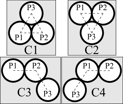
Figure 7: The canonical forms that we define for the four possible configurations in which three particles may undergo collision in 2 dimensions

Once the canonical configuration is chosen, all the velocities are rotated to reorient to the new axes. Total momenta and energy undergo a resultant change that can be reversed to recover original momenta and energy values simply by rotating the axes back to original axes. Since the original velocities are in a one-to-one relation with the transformed velocities, it is the transformed velocities that will be considered as velocities $a..f$ defined earlier for the 3-particle, 2-dimension collision model. After computing individual post-collision velocities, they are rotated back to the original frame of reference, thus restoring the original total momenta and energy.

4.5.2 Sampling the ${\bm{\Psi}}$ Phase Space

To generate a random set of offsets, ${\bm{\Psi}}$, a random sample point on the hyper-ellipsoid of Equation (29) is generated by invoking the numerical method given in Procedure 5 with $s=4$, and $\{{}_{4}\lambda_{i}\mid 1\leq i\leq 4\}$ obtained by converting Equation (29) into the canonical form expected by the algorithm. The sampling approach is a generalized version of the approach employed for 3-particle collisions in 1 dimension (Section 4.4) to sample the phase space of ${\bm{\Psi}}$. As mentioned earlier, although rejection-based methods are available for generating the samples, rejection is incompatible with reversibility, making them inapplicable here.

Procedure 5 (${\bm{G}}\longrightarrow{\bm{\Psi}}$): Generate the Parameters ${\bm{\Psi}}$ of a Random Point on the Surface of an $s$-Dimensional Hyper-Ellipsoid, ${\cal H}_{s}$, using Random Numbers ${\bm{G}}=\{G_{1},\ldots,G_{s-1}\}$

1:  Input: $s,\{{}_{s}\lambda_{i}\mid 1\leq i\leq s\}$, where integer $s>1$, and $\sum_{i=1}^{s}\left(\tfrac{{}x_{i}}{{}_{s}\lambda_{i}}\right)^{2}=1$ is the hyper-ellipsoid

2:  Output: $\{\psi_{i}\mid 1\leq i<s\}$, where $\psi_{i}$ are the parameters of a random point $({}_{r}x_{1},\ldots,{}_{r}x_{s})$ on the hyper-ellipsoid, such that ${}_{r}x_{i}={}_{s}\lambda_{i}\cos{\psi_{i}}\prod_{j=1}^{i-1}{\sin{\psi_{j}}}\text{ for all }1\leq i<s$, and ${}_{r}x_{s}={}_{s}\lambda_{s}\prod_{j=1}^{s}{\sin{\psi_{j}}}$

3:  for $k=s$ down-to $2$ do

4:     Let $\overline{k}=s-k+1$

5:     if $k=2$ then

6:        Invoke the algorithm in Section 4.4.3 using $G_{\overline{k}}$ to generate the parameter $0\leq\psi^{*}<2\pi$ corresponding to a random point on the perimeter of the (2-dimensional) ellipse ${\cal H}_{2}$

7:        $\psi_{\overline{k}}\leftarrow\psi^{*}$

8:     else

9:        Compute the surface area $A_{k}$ of ${\cal H}_{k}$

10:        Compute the random fraction ${}_{r}A_{k}$ of $A_{k}$ as: ${}_{r}A_{k}\leftarrow G_{\overline{k}}\cdot A_{k}$

11:        Using the bisection method analogous to that in Section 4.4.3, determine a $0\leq\psi^{*}\leq\pi$ such that surface area of the calotte of ${\cal H}_{k}$ defined by the latitudinal angle $\psi^{*}$ from the pole equals ${}_{r}A_{k}$

12:        $\psi_{\overline{k}}\leftarrow\psi^{*}$

13:        Determine the parameters $\{{}_{s-1}\lambda_{i}\mid 1\leq i\leq s-1\}$ of the $(s-1)$-dimensional ellipsoid ${\cal H}_{s-1}$ formed by the opening of the calotte, obtained by substituting ${}_{s}x_{\overline{k}}={}_{s}\lambda_{\overline{k}}\cos\psi_{\overline{k}}$.

14:     end if

15:  end for

Note that, by using one extra random number (i.e., using $d_{n}+1$ random numbers instead of $d_{n}$), Procedure 5 can be elegantly generalized, avoiding reliance on the separate algorithm of Section 4.4.3 for the special case of a 2-dimensional ellipsoid (ellipse). This can be achieved by iterating down to $s=1$, introducing an extra parameter $\psi_{s}$, and using the additional random number to set $\psi_{s}$ to either $\tfrac{\pi}{2}$ or $\tfrac{3\pi}{2}$ (i.e., ${}_{1}x_{1}=\pm{}_{1}\lambda_{1}$). Using such a generalized algorithm for sampling the surface of an $s$-dimensional ellipsoid, $s\geq 1$, the algorithm in Section 4.4.3 can be replaced by a call to the generalized Procedure 5 with $s=2$. However, to restrict the number of random numbers to $d_{n}$, we customize the last iteration to use the optimized version given in Section 4.4.3.

In the next sections, we derive the permissible ranges of the parameters, restricted from their full, nominal ranges due to conservation laws as well as geometrical constraints, and develop the forward and reverse collision procedures based on the derived parameter ranges.

4.5.3 Configuration C1

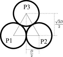
Figure 8: Measures of interest in configuration C1

From the geometry of C1 (ref. Figure 8), it can be seen that $r_{21x}=D$, $r_{21y}=0$, $r_{32x}=\tfrac{-D}{2}$, $r_{32y}=\tfrac{\sqrt{3}}{2}D$, $r_{13x}=\tfrac{-D}{2}$, and $r_{13y}=\tfrac{-\sqrt{3}}{2}D$. Using these in Equation (28) and Equation (31) to account for the geometrical constraints, we obtain the ranges of $\phi_{1}$ and $\phi_{2}$ that are more constrained than in Equation (30).

The inequality K1 directly gives the following:

$$D\cdot(\lambda\cos{\phi_{1}})+0\cdot(\cdots)>0$$ (34)

$$\implies\cos{\phi_{1}}\geq 0$$

$$\implies-\tfrac{\pi}{2}\leq\phi_{1}\leq\tfrac{\pi}{2}$$

$$\implies 0\leq\phi_{1}<\tfrac{\pi}{2}\text{ from Equation~{}(\ref{eqn:3sphere-2dim-ellipsoid-space}).}$$

Inequality K2 gives:

$$\tfrac{-D}{2}\cdot\left(\tfrac{\lambda}{{2}}(\sqrt{3}\sin{\phi_{1}}\sin{\phi_{2}}\cos{\phi_{3}}-\cos{\phi_{1}})\right)+$$ (35)

$$\tfrac{\sqrt{3}D}{2}\cdot\left(\tfrac{\lambda}{{2}}(\sqrt{3}\sin{\phi_{1}}\sin{\phi_{2}}\sin{\phi_{3}}-\sin{\phi_{1}}\cos{\phi_{2}})\right)>0.$$

$$\text{or, }-\sqrt{3}\sin{\phi_{1}}\sin{\phi_{2}}\cos{\phi_{3}}+\cos{\phi_{1}}+3\sin{\phi_{1}}\sin{\phi_{2}}\sin{\phi_{3}}-\sqrt{3}\sin{\phi_{1}}\cos{\phi_{2}}>0.$$

Inequality K3 gives:

$$\tfrac{-D}{2}\cdot\left(\tfrac{-\lambda}{{2}}(\sqrt{3}\sin{\phi_{1}}\sin{\phi_{2}}\cos{\phi_{3}}+\cos{\phi_{1}})\right)+$$ (36)

$$\tfrac{-\sqrt{3}D}{2}\cdot\left(\tfrac{-\lambda}{{2}}(\sqrt{3}\sin{\phi_{1}}\sin{\phi_{2}}\sin{\phi_{3}}+\sin{\phi_{1}}\cos{\phi_{2}})\right)>0.$$

$$\text{or, }\sqrt{3}\sin{\phi_{1}}\sin{\phi_{2}}\cos{\phi_{3}}+\cos{\phi_{1}}+3\sin{\phi_{1}}\sin{\phi_{2}}\sin{\phi_{3}}+\sqrt{3}\sin{\phi_{1}}\cos{\phi_{2}}>0.$$

From K2, we get:

L1: $$\cos(\phi_{3}+\tfrac{\pi}{3})<\tfrac{1}{2\sqrt{3}\tan\phi_{1}\sin\phi_{2}}-\tfrac{1}{2\tan\phi_{2}}.$$ (37)

Similarly, from K3, we get:

L2: $$-\cos(\phi_{3}-\tfrac{\pi}{3})<\tfrac{1}{2\sqrt{3}\tan\phi_{1}\sin\phi_{2}}+\tfrac{1}{2\tan\phi_{2}}.$$ (38)

To ensure a valid range for the left hand side in L1, the right hand side (RHS) of the same must not be less than $-1$. Setting the RHS to $-1$ defines the boundary between the possible and impossible regions, in terms of the relation between $\phi_{1}$ and $\phi_{2}$. Similar restrictions arise from L2. These considerations give the limits on $\phi_{1}$ and $\phi_{2}$ as follows:

$$\phi_{1} = \cot^{-1}(\sqrt{3}\cos\phi_{2}-2\sqrt{3}\sin\phi_{2}) -1$$ (from L1, RHS=) (39)

$$\phi_{1} = \cot^{-1}(-\sqrt{3}\cos\phi_{2}-2\sqrt{3}\sin\phi_{2}) \text{ (from {L2}, RHS=$-1$)}.$$

When $0\leq\phi_{1}\leq\phi_{1}^{*}=\tfrac{\pi}{6}$, $\phi_{2}$ is unrestricted in its range of $[0,\pi]$. When $\phi_{1}>\phi_{1}^{*}=\tfrac{\pi}{6}$, the lower- and upper bounds of $\phi_{2}$ are restricted, as determined next. Let $r=\tfrac{\cot\phi_{1}}{\sqrt{3}}$ (giving $r<1$ when $\tfrac{\pi}{6}<\phi_{1}<\tfrac{\pi}{2}$). Then, the lower bound $\phi_{2_{l}}\leq\phi_{2}$ is obtained by solving $r=\cos\phi_{2}-2\sin\phi_{2}$, giving $\phi_{2_{l}}=2\tan^{-1}(\tfrac{-2+\sqrt{5-r^{2}}}{1+r})$. Similarly, the upper bound $\phi_{2}\leq\phi_{2_{u}}$ is obtained by solving $r=-\cos\phi_{2}-2\sin\phi_{2}$, giving $\phi_{2_{u}}=2\tan^{-1}(\tfrac{+2+\sqrt{5-r^{2}}}{1-r})$.

Also, the values of $\phi_{1}$ and $\phi_{2}$ could restrict the range of $\phi_{3}$, whose limits are obtained by setting the RHS to unity. The restrictions on $\phi_{3}$ are obtained from:

$$\phi_{1} = \cot^{-1}(\sqrt{3}\cos\phi_{2}+2\sqrt{3}\sin\phi_{2})$$ (from L1, RHS=1) (40)

$$\phi_{1} = \cot^{-1}(-\sqrt{3}\cos\phi_{2}+2\sqrt{3}\sin\phi_{2}) \text{ (from {L2}, RHS=1)}.$$

All the limiting curves on the angles are illustrated in Figure 9, which shows the space spanned by the nominal ranges of $\phi_{1}\in[0,\tfrac{\pi}{2}]$ and $\phi_{2}\in[0,\pi]$. The space is divided into six different regions that impose different constraints on the ranges of $\phi_{1}$, $\phi_{2}$ and $\phi_{3}$. The first two regions, labeled ${\bm{R}^{-}_{0}}$ and ${\bm{R}^{-}_{\pi}}$, demarcate the regions excluded to make RHS$>-1$ (Equation (39)), one on each side of $\phi_{2}=0$ and $\phi_{2}=\pi$. In the region marked ${\bm{R}^{+}_{0}}$, the range of $\phi_{3}$ is restricted from below to be greater than 0, and in the region marked ${\bm{R}^{+}_{\pi}}$, the range of $\phi_{3}$ is restricted from the above to be less than $2\pi$. In the region marked ${\bm{R}^{-}_{-}}$, $\phi_{3}$ is restricted from both below and above. The appropriate lower bound $\phi_{3_{l}}$, and upper bound $\phi_{3_{u}}$ on $\phi_{3}$ can be computed accordingly. In the region marked ${\bm{R}^{+}_{+}}$, $\phi_{3}$’s original range of $[0,2\pi)$ is unrestricted.

Thus, for C1, the ranges for post-collision parameters are:

$$\phi_{1} \in[0,\tfrac{\pi}{2})$$ (41)

$$\phi_{2} \in\left\{\begin{aligned} [0,0]&\text{ if }\phi_{1}=0\\ [0,\pi]&\text{ if }0<\phi_{1}\leq\tfrac{\pi}{6}\\ [\phi_{2_{l}},\phi_{2_{u}}]&\text{ otherwise }(\textit{i.e.},\tfrac{\pi}{6}<\phi_{1}<\tfrac{\pi}{2})\end{aligned}\right.$$

$$\phi_{3} \in\left\{\begin{aligned} [0,0]&\text{ if }\phi_{1}=0\text{ or }\phi_{2}=0\text{ or }\phi_{2}=\pi\\ [\phi_{3_{l}},\phi_{3_{u}}]&\text{ if ($\phi_{1}$,$\phi_{2}$) falls in ${\bm{R}^{+}_{0}}$, ${\bm{R}^{+}_{\pi}}$ or ${\bm{R}^{-}_{-}}$}\\ [0,2\pi)&\text{ otherwise ({i.e.}, ($\phi_{1}$,$\phi_{2}$) falls in ${\bm{R}^{+}_{+}}$).}\end{aligned}\right.$$

Figure 9: Regions in the nominal phase spaces of $\phi_{1}$ and $\phi_{2}$ demarcating different bounds of $\phi_{1}$, $\phi_{2}$, and $\phi_{3}$ in Configuration 1 of 3-particle collisions in 2 dimensions

Using a similar analysis, the pre-collision ranges can be obtained, as illustrated in Figure 9, which shows the range of $\phi_{1}^{{}^{\prime}}\in(\tfrac{\pi}{2},\pi]$, and corresponding constraints of $\phi_{2}^{{}^{\prime}}$ and $\phi_{2}^{{}^{\prime}}$ in terms of the forward regions ${\bm{F}_{0}^{-}}$, ${\bm{F}_{\pi}^{-}}$, and so on.

The forward and reverse procedures for this configuration are given in Procedure 6 and Procedure 7 respectively.

Procedure 6 ($(\phi_{1}^{{}^{\prime}},\phi_{2}^{{}^{\prime}},\phi_{3}^{{}^{\prime}})\longrightarrow(\phi_{1},\phi_{2},\phi_{3})$): Forward Procedure for Configuration 1 of a 3-Particle Collision in 2 dimensions

1:  Invoke Procedure 5 to generate the parameters $(\psi_{1},\psi_{2},\psi_{3})$ of a random point on surface of the hyper-ellipsoid represented by Equation (29)

2:  $\phi_{1}\leftarrow(\phi_{1}^{{}^{\prime}}-\tfrac{\pi}{2}+\psi_{1})\mod\tfrac{\pi}{2}$

3:  $\phi_{2}\leftarrow(\phi_{2}^{{}^{\prime}}+\psi_{2})\mod\pi$

4:  Compute $\phi_{2_{l}}$ and $\phi_{2_{u}}$ {based on $\phi_{1}$}

5:  if $\phi_{2}<\phi_{2_{l}}$ or $\phi_{2_{u}}<\phi_{2}$ then

6:     $\phi_{2}\leftarrow(\phi_{2}+(\phi_{2_{l}}+\pi-\phi_{2_{u}}))\mod\pi$

7:  end if

8:  Compute $\phi_{3_{l}}$ and $\phi_{3_{u}}$ {based on $\phi_{1}$ and $\phi_{2}$}

9:  $\phi_{3}\leftarrow(\phi_{3}^{{}^{\prime}}+\psi_{3})\mod 2\pi$

10:  if $\phi_{3}<\phi_{3_{l}}$ then

11:     $\phi_{3}\leftarrow(\phi_{3}+\phi_{3_{l}})\mod 2\pi$

12:  else if $\phi_{3}>\phi_{3_{u}}$ then

13:     $\phi_{3}\leftarrow(\phi_{3}+(2\pi-\phi_{3_{u}}))\mod 2\pi$

14:  end if

Procedure 7 ($(\phi_{1},\phi_{2},\phi_{3})\longrightarrow(\phi_{1}^{{}^{\prime}},\phi_{2}^{{}^{\prime}},\phi_{3}^{{}^{\prime}})$): Reverse Procedure for Configuration 1 of a 3-Particle Collision in 2 dimensions

1:  Invoke Procedure 5 to re-generate the parameters $(\psi_{1},\psi_{2},\psi_{3})$ of the random point on surface of the hyper-ellipsoid represented by Equation (29), previously generated by Procedure 6

2:  Recompute $\phi_{2_{l}}$ and $\phi_{2_{u}}$ {based on $\phi_{1}$}

3:  Recompute $\phi_{3_{l}}$ and $\phi_{3_{u}}$ {based on $\phi_{1}$ and $\phi_{2}$}

4:  $\phi_{1}^{{}^{\prime}}\leftarrow\tfrac{\pi}{2}+((\phi_{1}-\psi_{1})\mod\tfrac{\pi}{2})$

5:  $\phi_{2}^{{}^{\prime}}\leftarrow(\phi_{2}-\psi_{2})\mod\pi$

6:  if $\phi_{2}^{{}^{\prime}}<\phi_{2_{l}}$ or $\phi_{2_{u}}<\phi_{2}^{{}^{\prime}}$ then

7:     $\phi_{2}^{{}^{\prime}}\leftarrow(\phi_{2}^{{}^{\prime}}-(\phi_{2_{l}}+\pi-\phi_{2_{u}}))\mod\pi$

8:  end if

9:  $\phi_{3}^{{}^{\prime}}\leftarrow(\phi_{3}-\psi_{3})\mod 2\pi$

10:  if $\phi_{3}^{{}^{\prime}}<\phi_{3_{l}}$ then

11:     $\phi_{3}^{{}^{\prime}}\leftarrow(\phi_{3}^{{}^{\prime}}-\phi_{3_{l}})\mod 2\pi$

12:  else if $\phi_{3}^{{}^{\prime}}>\phi_{3_{u}}$ then

13:     $\phi_{3}^{{}^{\prime}}\leftarrow(\phi_{3}^{{}^{\prime}}-(2\pi-\phi_{3_{u}}))\mod 2\pi$

14:  end if

4.5.4 Configuration C2

Using algebra similar to that for C1, the ranges for configuration C2 are obtained, with swapped signs for $r_{32y}$ and $r_{13y}$.

4.5.5 Configuration C3

Configuration C3 can be parameterized by an angle $\theta$ that P3 makes relative to P2, as shown in Figure 10.

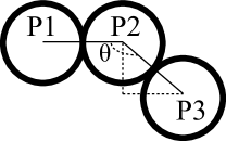
Figure 10: Parametrization of configuration C3 by angle $\theta$, $\tfrac{\pi}{3}<\theta<\tfrac{5\pi}{3}$

In this configuration, $r_{21x}=D$, $r_{21y}=0$ (as was the case for C1 and C2), but $r_{32x}=-D\cos{\theta}$, $r_{32y}=-D\sin{\theta}$, and we are not concerned about $r_{13x}$ and $r_{13y}$. Using these in Equation (28), we get the geometrically constrained ranges of $\phi_{1}$, $\phi_{2}$, and $\phi_{3}$. Since the inquality K1 for this configuration is the same as for configurations C1 and C2, the range of $\phi_{1}$ remains $(0,\tfrac{\pi}{2}]$. However, only the inequality K2 applies to this configuration, and K3 need not apply. From K2, we get:

$$-D\cos\theta\tfrac{\lambda}{{2}}(\sqrt{3}\sin\phi_{1}\sin\phi_{2}\cos\phi_{3}-\cos\phi_{1})$$

$$-D\sin\theta\tfrac{\lambda}{{2}}(\sqrt{3}\sin\phi_{1}\sin\phi_{2}\sin\phi_{3}-\sin\phi_{1}\cos\phi_{2})>0\text{ .}$$

Since $\sin\phi_{1}\neq 0$ and $\sin\phi_{2}\neq 0$,

$$\cos(\phi_{3}-\theta)\sqrt{3}\sin\phi_{1}\sin\phi_{2}<\cos\theta\cos\phi_{1}+\sin\theta\sin\phi_{1}\cos\phi_{2}$$ (42)

$$\implies \cos(\phi_{3}-\theta)<\gamma\text{, where }$$

$$\gamma=\dfrac{\cos\theta\cos\phi_{1}+\sin\theta\sin\phi_{1}\cos\phi_{2}}{\sqrt{3}\sin\phi_{1}\sin\phi_{2}}$$

$$\implies \phi_{3}\in[\phi_{3_{l}}+\theta,\phi_{3_{u}}+\theta]\text{, where}$$

$$0\leq(\phi_{3_{l}}+\theta)\bmod{2\pi}\leq(\phi_{3_{u}}+\theta)\bmod{2\pi}\leq 2\pi\text{, and }$$

$$\phi_{3_{l}}\text{ and }\phi_{3_{u}}\text{ are solutions to }\cos^{-1}\gamma.$$

Also, the range of $\phi_{2}$ may be constrained due to the requirement that $-1\leq\gamma\leq 1$. Let $\mu=\tfrac{\cos\theta}{\sqrt{3}\tan\phi_{1}}$ and $\nu=\tfrac{\sin\theta}{\sqrt{3}}$. Then, $\gamma=\tfrac{\mu+\nu\cos\phi_{2}}{\sin\phi_{2}}$. If $\mu-\nu\geq 0$ or $\mu+\nu\leq 0$, then the range of $\phi_{2}$ is not constrained, giving the lowerbound $\phi_{2_{l}}\leq\phi_{2}$ equal to 0 and upperbound $\phi_{2}\leq\phi_{2_{u}}$ equal to $\pi$. Otherwise, the lower bound (greater than $0$) and upper bound (less than $\pi$) of $\phi_{2}$ must be determined as follows.

If $\mu-\nu<0$, the lowerbound of $\phi_{2}$ is obtained by solving for $\phi_{2}$ in $-\sin\phi_{2}=\mu+\nu\cos\phi_{2}$. Since $\sin\phi_{2}$ and $\mu+\nu\cos\phi_{2}$ intersect in at most two points within the range $(0,\pi)$ (see Figure 11), a unique lowerbound $\phi_{2_{l}}$, $0<\phi_{2_{l}}\leq\phi_{2}<\pi$ is obtainable. Similarly, if $\mu+\nu>0$, then a unique upperbound $\phi_{2_{u}}$, $0<\phi_{2}\leq\phi_{2_{u}}<\pi$ is obtained by solving for $\phi_{2}$ in $\sin\phi_{2}=\mu+\nu\cos\phi_{2}$.

Figure 11: Illustration of lower and upper bounds of $\phi_{2}$ in configuration 3 of 3-particle collisions in 2 dimensions

Thus, for C3, the ranges are:

$$\phi_{1} \in[0,\tfrac{\pi}{2})$$ (43)

$$\phi_{2} \in\left\{\begin{aligned} [0,0]&\text{ if }\phi_{1}=0\\ [0,\pi]&\text{ if }\mu-\nu\geq 0\text{ or }\mu+\nu\leq 0\\ [\phi_{2_{l}},\phi_{2_{u}}]&\text{ otherwise }\end{aligned}\right.$$

$$\phi_{3} \in\left\{\begin{aligned} [0,0]&\text{ if }\phi_{1}=0\text{ or }\phi_{2}=0\text{ or }\phi_{2}=\pi\\ [\phi_{3_{l}}+\theta,\phi_{3_{u}}+\theta]&\text{ otherwise.}\end{aligned}\right.$$

The ranges may be derived similarly for pre-collision. The range of $\phi_{1}^{{}^{\prime}}$ remains to be the same as in configuration 1 at $(\tfrac{\pi}{2},\pi]$, but, Equation (42) changes to $\cos{(\phi_{3}^{{}^{\prime}}-\theta)}>\gamma$.

4.5.6 Configuration C4

The treatment of configuration C4 proceeds similar to that for configuration C3, using K3 instead of K2.

4.6 Random Number Generation

A subtle but important consideration in zero-memory reversal is the need to ensure that the exact number of random number invocations is also recovered during reverse execution without explicitly storing that information. In other words, the number of random numbers thrown, $G_{C}$, for any collision $C$ must be determinable by the collision operator such that the random number sequence is correctly reinstated to the proper position corresponding to the pre-collision state. All our algorithms possess this property, with $G_{C}=d_{n}$.

In the case of 2-particle collisions in 1 dimension, no random numbers are needed, trivially satisfying the property. In the case of 2-particle collisions in 2 dimensions, exactly one random number is generated per collision (Procedure 1), and hence the random number stream is stepped back by exactly one number during reversal of that collision (Procedure 2).

The case of 2-particle collisions in 3 dimensions is slightly more complex, since it requires more than one random number to be generated. For forward collision, it appears possible to sometimes generate one random number and some other times two. Only one random number (let us denote it by $G_{1}$) appears sufficient to be generated if that number happens to result in $\phi_{1}=0$ or $\phi_{1}=\pi$. Similarly, two random numbers (let us denote them by $G_{1}$ and $G_{2}$) appear needed only to generate $\phi_{2}$ if the randomly generated $\phi_{1}$ (from $G_{1}$) is such that $\phi_{1}\neq 0$ and $\phi_{1}\neq\pi$. However, this conditional generation of one or two random numbers per collision creates difficulties during reversal, because, when the random number stream is reversed and the previous random number $G$ is recovered, we will remain unsure whether $G$ corresponds to $G_{1}$ or $G_{2}$. It is impossible to disambiguate between the two possibilities because both $\phi_{1}$ and $\phi_{2}$ may assume the value of zero. Hence, we would remain unsure if, in the forward collision, $G_{1}$ was zero and hence $G_{2}$ was not used for that collision, or if $G_{1}$ happened to be non-zero and $G_{2}=G$ happened to be zero. Similar ambiguity can be argued for the case of $G\neq 0$. Due to these considerations, we fix the number of random numbers generated per forward collision to be exactly two, unconditionally, so that the random number stream can be reversed exactly by two, restoring it to the correct pre-collision state. If $G_{1}$ results in $\phi_{1}=0$, $G_{2}$ is still generated from the stream, but simply discarded by the collision algorithm. Assuming that the stream is random, the discarding of $G_{2}$ when $\phi_{1}=0$ does not affect the uniformity of the random samples. Note that the discarding is performed unconditionally, without any dependence or usage of the actual value of the discarded $G_{2}$ in the forward model. This aspect of unconditional discarding is crucial for reversal, because the reversal also can determinstically reverse the random number stream.

For 3-particle collisions in 1 dimension, exactly one random angle is required for every forward collision, and hence one reversal is necessary and sufficient in each reverse collision, ensuring correct reversal of the random stream. For 3-particle collisions in 2 dimensions (Appendix 4.5), one, two, or three random angles are needed (depending on the geometry and pre-collision velocities) per forward collision. However, due to considerations similar to those for the case of 2-particle collisions in 3 dimensions, we use exactly three random numbers for every forward collision (even if only one or two of them may be sufficient in special cases of dynamics and geometry) in order to reverse the random number stream correctly.

In general, exactly $d_{n}$ random numbers must be generated for every collision involving $n$ particles in $d$ dimensions.

With regard to the number of distinct streams to employ in the simulation, it is possible to use one of the following three approaches: (1) a single random number stream for the entire system, or (2) $N$ independent streams, corresponding to each particle in the system, or (3) $d_{n}$ independent streams for use in each collision. The first approach clearly requires a very high quality random number generator with a very long period in order to support a large number of collisions when $N$ is large. The second approach requires relatively smaller periods per stream but also requires minimal correlation between streams. In any given collision, the random stream of the particle with the smallest identifer among the colliding particles can be used for that collision. The third approach can be used to sample exactly one random number per stream per collision. All approaches seem appropriate for reversal, depending on the modeler’s specific needs regarding computational cost and the stream period.

Another context in which reversibility considerations of random number streams plays an important role is in generating random samples of ${\bm{\Psi}}$. The ${\bm{G}}$-to-${\bm{\Psi}}$ function for sampling ${\bm{\Psi}}$ involves sampling the circumference of an ellipse (or, in general, sampling the points on the surface of higher dimensional ellipsoids). While rejection-based sampling procedures [PTVF07] are available for such problems, they cannot be used in reversible execution. This is because the number of (uniformly distributed) random numbers used by such rejection-based procedures varies with each sampled point, which makes it impossible to unambiguously reverse the random number stream without keeping track of how many random numbers were generated for each sample. In fact, rejection-based sampling can only be employed for certain special classes of probability distributions, whose parametric input does not vary across samples [PD09], whereas, in sampling ${\bm{\Psi}}$, the parametric input varies with each collision.

5 Implementation Results

In order to test the performance of the algorithms, we implemented the algorithms in software using the C++ programming language, and executed simulation experiments. The experiments are intended to test (1) the ability to restore the initial state after a sequence of many forward collisions followed by their reversals, and (2) the quality of phase space coverage discerned from the uniformity of generated velocity samples. For random number generation, we used a reversible version of a high quality linear congruential generator [LA97] with a period of $2^{121}$. A single generator stream is used for all the particles. In each configuration, the experiments verify successful reversal across several thousands of collisions.

5.1 Collision Sequence Reversal

Procedure 8 Reversal Illustration for 2-Particle Collisions in 2 Dimensions

1:  $(a,b,c,d)\leftarrow(a_{0},b_{0},c_{0},d_{0})$ {initial velocities}

2:  $\alpha\leftarrow a+b$, $\beta\leftarrow c+d$, $\delta\leftarrow a^{2}+b^{2}+c^{2}+d^{2}$ {momenta and energy}

3:  $S\leftarrow$ random number seed

4:  $r_{21x}\leftarrow 1$, $r_{21y}\leftarrow 1$ {normalized collision geometry}

5:  for $i=1$ to $N_{c}$ do {$\---$ Forward Execution $\---$}

6:     $\phi_{1}^{{}^{\prime}}\leftarrow{\bm{V\text{-to-}\Phi}}(a,b,c,d)$ of Section 4.2

7:     $G\leftarrow{\bm{RNG}}(S)$ {Generate next random number in $[0,1)$}

8:     $\phi_{1}\leftarrow$ Apply Procedure 1 on $\phi_{1}^{{}^{\prime}}$ using $G$, $r_{21x}$, and $r_{21y}$

9:     $(a,b,c,d)\leftarrow{\bm{\Phi\text{-to-}V}}(\alpha,\beta,\delta,\phi_{1})$ of Section 4.2

10:     $a\leftarrow-a$, $b\leftarrow-b$, $c\leftarrow-c$, $d\leftarrow-d$ {Reverse velocities to create next collision}

11:  end for

12:  for $i=N_{c}$ to $1$ do {$\---$ Reverse Execution $\---$}

13:     $a\leftarrow-a$, $b\leftarrow-b$, $c\leftarrow-c$, $d\leftarrow-d$

14:     $\phi_{1}\leftarrow{\bm{V\text{-to-}\Phi}}(a,b,c,d)$ of Section 4.2

15:     $G\leftarrow{\bm{RNG^{-1}}}(S)$ {Recover previous random number}

16:     $\phi_{1}^{{}^{\prime}}\leftarrow$ Apply Procedure 2 on $\phi_{1}$ using $G$, $r_{21x}$, and $r_{21y}$

17:     $(a,b,c,d)\leftarrow{\bm{\Phi\text{-to-}V}}(\alpha,\beta,\delta,\phi_{1}^{{}^{\prime}})$ of Section 4.2

18:  end for

19:  if $a=a_{0}$ and $b=b_{0}$ and $c=c_{0}$ and $d=d_{0}$ then {$\---$ Verification $\---$}

20:     print  ’Passed’

21:  end if

Procedure 9 Reversal Illustration for 3-Particle Collisions in 1 Dimension

1:  $(a,b,c)\leftarrow(a_{0},b_{0},c_{0})$ {initial velocities}

2:  $\alpha\leftarrow a+b+c$, $\delta\leftarrow a^{2}+b^{2}+c^{2}$ {momenta and energy}

3:  $S\leftarrow$ random number seed

4:  for $i=1$ to $N_{c}$ do {$\---$ Forward Execution $\---$}

5:     $\phi_{1}^{{}^{\prime}}\leftarrow{\bm{V\text{-to-}\Phi}}(a,b,c)$ of Section 4.4

6:     $G\leftarrow{\bm{RNG}}(S)$ {Generate next random number in $[0,1)$}

7:     $\phi_{1}\leftarrow$ Apply Procedure 3 on $\phi_{1}^{{}^{\prime}}$ using $G$

8:     $(a,b,c)\leftarrow{\bm{\Phi\text{-to-}V}}(\alpha,\delta,\phi_{1})$ of Section 4.4

9:     $a\leftarrow-a$, $b\leftarrow-b$, $c\leftarrow-c$ {Reverse velocities to create next collision}

10:  end for

11:  for $i=N_{c}$ to $1$ do {$\---$ Reverse Execution $\---$}

12:     $a\leftarrow-a$, $b\leftarrow-b$, $c\leftarrow-c$

13:     $\phi_{1}\leftarrow{\bm{V\text{-to-}\Phi}}(a,b,c)$ of Section 4.4

14:     $G\leftarrow{\bm{RNG^{-1}}}(S)$ {Recover previous random number}

15:     $\phi_{1}^{{}^{\prime}}\leftarrow$ Apply Procedure 4 on $\phi_{1}$ using $G$

16:     $(a,b,c)\leftarrow{\bm{\Phi\text{-to-}V}}(\alpha,\delta,\phi_{1}^{{}^{\prime}})$ of Section 4.4

17:  end for

18:  if $a=a_{0}$ and $b=b_{0}$ and $c=c_{0}$ then {$\---$ Verification $\---$}

19:     print  ’Passed’

20:  end if

Procedure 8 shows the pseudocode of the experiment program for 2-particle collisions in 2 dimensions. Procedure 9 shows the pseudocode of the experiment program for 3-particle collisions in 1 dimension. In both, the state of the particles is initialized to any desired intial configuration, followed by a sequence of $N_{c}$ applications of the forward collision operator. ${\bm{RNG}}(S)$ represents the generation of the next sample in $[0,1)$ from the random number stream (which also updates $S$ as side-effect), while ${\bm{RNG^{-1}}}(S)$ represents the reversal of the most previous invocation to ${\bm{RNG}}$ and the recovery of the most recently generated value from ${\bm{RNG}}$. After each forward collision, post-collision velocities are multiplied by $-1$ to give the new pre-collision velocities for the next collision. Since the post-collision velocities are guaranteed to be divergent, their opposites are guaranteed to give converging velocities that will result in the next collision. After all $N_{c}$ forward collisions, the entire sequence is reversed by executing the reverse collision operator $N_{c}$ times. Clearly, the reversal is successful if the final velocities after all $N_{c}$ reversals recovers the initial velocities. This condition is verified at the end and the corresponding status message is printed.

All executions terminated successfully with a “passed” status, verifying the restoration of initial state after reversal of $N_{c}$ collisions. The unbiased and correct phase space coverage is tested with $N_{c}$ up to $10^{6}$ by plotting the post-collision angles against random angle offsets and pre-collision velocities.

In the case of 3-particle collisions in 1 dimension, numerical integration to compute the segment length of an ellipse was performed using the Simpson’s rule. Also, care was needed to account for numerical precision issues when using the numerically computed cosine function, which sometimes produces numerical noise for angles within very small neighborhoods of multiples of $\tfrac{\pi}{6}$ and $\tfrac{\pi}{2}$. A tolerance of $\pm 10^{-8}$ around zero was employed when determining whether any given cosine value can be considered zero or positive.

Figure 12: Sampling for $N_{c}=10^{4}$ collisions in 2-particle collisions in 2 dimensions

Figure 13: Sampling for $N_{c}=10^{4}$ collisions in 3-particle collisions in 1 dimension

Figure 5.1 plots the post-collision angles against their corresponding pre-collision angles generated as part of an execution of 2-particle collisions in 2 dimensions, and plots the post-collision angles against their corresponding random angles in the same execution. Both plots show excellent uniformity and correctness of the sampled phase space. Similarly, Figure 5.1 shows the corresponding data for 3-particle collisions in 1 dimension; again, they display excellent coverage. Since the covered areas in the plots become too dense for visual clarity when $N_{c}$ becomes large, only data for $N_{c}=10^{4}$ are shown in the figures .

5.2 Randomness Tests

The correctness of phase space coverage is experimentally verified by testing the randomness of the generated angles using statistical tests. The Diehard Battery of Tests [Mar95] for statistical verification of randomness is used for this purpose.

The post-collision angles are mapped to double-precision numbers, each in $[0,1)$, and the uniformity of their distribution is verified. This method is applied to 2-particle collisions in 2 dimensions, and to 3-particle collisions in 1 dimension.

For 2-particle collisions in 2 dimensions, each post-collision angle $\phi_{1}$ is mapped to a double-precision number $\eta\in[0,1)$ as $\eta={(\phi_{1}-\kappa)}/{\pi}$, where $\kappa=0$ if $0\leq\phi_{1}\leq\tfrac{\pi}{2}$, and $\kappa=\pi$ otherwise ($\tfrac{3\pi}{2}\leq\phi_{1}\leq 2\pi$). Each $\eta$ is converted into an integer equal to $\lfloor{\eta\times 4,294,967,296}\rfloor$, and the resulting series of numbers (in hexadecimal format) is converted via the asc2bin program of Diehard to a binary-formatted file given as input to the diehard program.

For 3-particle collisions in 1 dimension, each post-collision angle $\phi_{1}$ is mapped to a double-precision number $\eta\in[0,1)$ as $\eta={(\phi_{1}-\tfrac{7\pi}{6})}/{(\tfrac{3\pi}{2}-\tfrac{7\pi}{6})}$. Each $\eta$ is converted into an integer equal to $\lfloor{\eta\times 4,294,967,296}\rfloor$, and the resulting series of numbers (in hexadecimal format) is converted via the asc2bin program of Diehard to a binary-formatted file given as input to the diehard program.

Both Procedure 8 and Procedure 9 were successfully executed with $N_{c}=3,000,000$ collisions, such that they terminate with a “Passed” result. The angles are logged to a file during their execution, and then used as input to the randomness tests. According to the Diehard tests, if the “$p$-values” computed and printed by diehard are observed to be strictly greater than 0 and less than unity, randomness is understood to be satisfied [Mar95]. The $p$-values observed from the randomness tests on the generated angles are given in Table 1. Good phase space coverage via randomization is indicated by the fact that the $p$-values from several tests are significantly away from zero and unity.

For 2-particle collisions in 2 dimensions, all tests in the Diehard repository were used and verified to generate very good randomness (positive $p$-values less than unity) without exception. This is due to the fact that no numerical precision effects are present in the collision algorithm for 2-particle collisions in 2 dimensions. For 3-particle collisions in 1 dimension, all tests were used except those that operate on bit-level representations (such as the Birthday, Bitstream and Count-the-1s tests). This is because round off and trunction effects in numerical integration, even at a relatively high precision of $10^{-9}$ in the computation of angles, introduces non-random patterns in the last few bits of the mantissa, appearing as non-randomness when selectively viewed in isolation or across multiple floating point numbers. However, when the angles are viewed as numbers themselves, uniform randomness is indeed observed, as expected.

Table 1: Randomness indicator $p$-values from Diehard battery of tests

Test	Category	$p$-value
		2-Dimension	1-Dimension
		2-Particle	3-Particle
CRAPS	Overall	0.979800	0.570270
	Wins	0.790715	0.862293
	Throws/game	0.979797	0.570273
RUNS	Set 1 - Up	0.847070	0.298998
	Set 1 - Down	0.128221	0.632054
	Set 2 - Up	0.183069	0.871807
	Set 2 - Down	0.244909	0.111657
SUMS	10 $\chi^{2}$-tests on 100 $\chi^{2}$-tests	0.370145	0.257959
SQUEEZE	42 degrees of freedom	0.890107	0.435410
3DSPHERES	$\chi^{2}$-test on 20 $p$-values	0.813199	0.897844
MINDIST	$\chi^{2}$-test on 100 min-distances	0.348209	0.751603
PARKLOT	$\chi^{2}$-test on 10 $p$-values	0.947200	0.720233

6 Performance Estimation

To estimate the performance gain that can be expected by resorting to reversible collisions instead of state saving, we implemented a simulation of a sequence of 2-particle collisions in a closed system of $N$ particles in $d=2$ dimensions. Experiments were run with $N=1,000$, $N=10,000$, and $N=100,000$ particles. Starting with random initial configuration of positions and velocities, and randomly selected inter-collision times, particle motion is simulated between collisions, and, at every collision point, the collision operator is applied on a random pair of particles. With state saving, the system state is saved to memory before every collision, to be able to roll back to that state. With reverse computation, no state is saved, as the system can be rolled back perfectly to any point in the past by reverse computation alone, without reliance on memory.

Two platforms with different computational and memory characteristics are tested: one with traditional central processing unit (CPU), and the other with newer graphical processing unit (GPU). Modern CPUs now have much higher computational speeds than memory speeds; the differential between computational and memory speeds is even more pronounced in modern GPU platforms [PFS05]. Implementation on the CPU is realized in the C++ programming language, and that on the GPU is in the CUDA programming language [SK10]. The CPU is an AMD Opteron 6174 processor with 64 GB of memory. The GPU is a high-end nVidia Geforce GTX 580 (Fermi) accelerator with 512 CUDA cores and 3 GB device memory. Compilation systems used were gcc 4.4.5 and CUDA 4.1.

In each simulation run, $N_{c}=1000$ collisions were simulated, and, after $N_{c}$ collisions, the system was rolled back to the beginning. With reverse computation, the positions and velocities are verified to match the initial conditions exactly (to within at least $\epsilon=\pm 10^{-9}$), while, with state saving, the results are trivially exactly matched.

The results are drawn as stacked histograms in Figure 14, with the total height of each bar representing the total time for forward execution of $N_{c}$ collisions and their reversal, which is split into Forward Time and Rollback Time in milliseconds. Three variants are benchmarked: SS1 represents the state saving mechanism in which all state is saved (positions and velocities); SS2 represents an optimized state saving mechanism in which the positions are saved and only the four components of the pre-collision velocities of the colliding pair are saved; RC represents the reverse computation with no memory. For each variant, the suffix -CPU represents execution on the CPU, and -GPU represents execution on the GPU.

CPU-based implementation	GPU-based implementation
(a)              Number of particles = 1,000              (b)
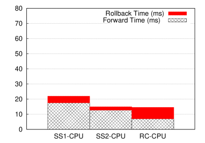
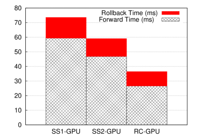
(c)              Number of particles = 10,000              (d)
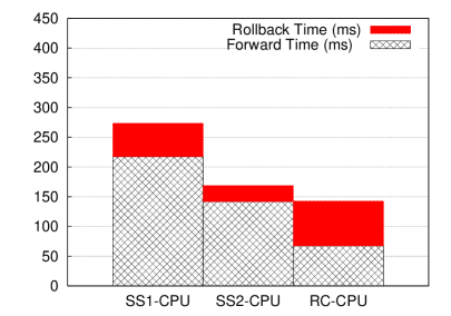
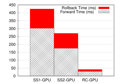
(e)              Number of particles = 100,000              (f)

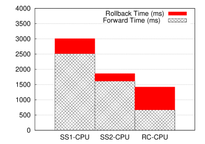
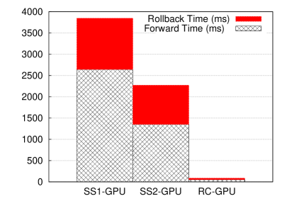
Figure 14: Performance of state saving and reverse computation with $N_{c}=1000$ collisions

Total run time with reverse computation is lower across the board. As expected, the greatest differential is observed in Figure 14(f) for the GPU runs with the largest number of particles ($N=100,000$). Since the ratio of memory transfer cost to computational cost is much higher with the GPU, reverse computation runs much faster, while state saving incurs the high memory transfer cost for every collision. Also, the GPU platform is known to be extremely efficient with large vectorized codes such as this simulation (i.e., more particles can be simulated with little increase in total time, if memory bottle neck is relieved). Hence, the reverse computation runs are extremely fast on the GPU, compared to all CPU runs and also compared to state saving with GPU. On smaller number of particles ($N=1000$ and $N=10,000$), CPU runs in (a) and (c) are faster than GPU runs in (b) and (d) because of larger CPU caches, yet, even in this case of relatively lower memory cost, reverse computation is observed to run faster. Even more importantly, when the number of particles is further increased (e.g., $N\geq 1\text{ million}$), state saving becomes infeasible due to memory limitations, but reverse computation runs well even at such large scale. Similarly, the benefit of using reversible simulation only increases with increase in the number of collisions, due to corresponding increase in the memory needs of state saving. A more detailed analysis of the memory subsystem behavior (e.g., data cache misses at levels 1 and 2, and translation lookaside buffer metrics) for each of these runs is part of our planned future work.

7 Summary

The classical problem of simulating elastic collisions of hard spheres has been revisited, with the important additional requirement of reversibility. Although classical simulation of elastic collisions has been well studied in the literature, little has been known on how to simulate them reversibly with minimal memory overhead. Here, we formalized the problem in terms of accurate phase space coverage specification and geometrical constraints. We solved the problem by developing a general framework that combines reversible pseudo random number generation with new mapping functions, geometrical constraints, and reversal semantics. While previous log-based approaches require memory proportional to the number of collisions, our algorithms incur essentially zero memory overheads and also ensure correct phase space coverage. We developed the detailed steps for 2-particle collisions (up to 3 dimensions) and 3-particle collisions (up to 2 dimensions). In these configurations, memory overhead is exactly zero for collisions in which $d_{n}=1$, and essentially zero for collisions with $d_{n}>1$. In the latter configurations, $\{\phi_{i+1}^{{}^{\prime}},\ldots,\phi_{d_{n}}^{{}^{\prime}}\}$ are logged if and only if $\phi_{i}=0$, for any $1\leq i<d_{n}$. Generalizations to collisions among larger number of particles and at higher dimensions are tedious, but can be carried out if needed. At higher dimensions and with larger number of particles, computationally expensive numerical integration becomes necessary in both classical (forward-only) approaches as well as in the forward procedures of our reversible method. To meet the goal of minimal memory overhead, our reverse procedures rely on numerical integration as well, whereas log-based reversal approaches would use memory to save information and avoid recomputation in the reverse path. In a normal, well-balanced parallel execution, reversals of collisions are far fewer than forward collisions (i.e., dependency violations are incurred infrequently). In such cases, our reversible models are more efficient, since forward cost for reversibility is eliminated, whereas log-based approaches would incur log-generation costs in forward execution.

Finally, although reversibility of elastic collisions is a seemingly simple problem to formulate, it includes sufficient complexity to make it challenging. The new approach and results presented here offer insights in revisiting additional classical physical system models with the added requirement of reversibility and exploring their fundamental memory characteristics and limits.

Acknowledgements

This paper has been authored by UT-Battelle, LLC, under contract DE-AC05-00OR22725 with the U.S. Department of Energy. Accordingly, the United States Government retains and the publisher, by accepting the article for publication, acknowledges that the United States Government retains a non-exclusive, paid-up, irrevocable, world-wide license to publish or reproduce the published form of this manuscript, or allow others to do so, for United States Government purposes. Research was partly supported by the DOE Early Career Award in Advanced Scientific Computing Research under grant number 3ERKJR12. The authors thank Alfred J. Park, Sudip K. Seal, and James J. Nutaro for constructive comments on early versions of the manuscript, and Alfred J. Park for helping with the implementation for performance estimation.

References

- [HBD+89] P. Hontalas, B. Beckman, M. DiLorento, L. Blume, P. Reiher, K. Sturdevant, L. V. Warren, J. Wedel, F. Wieland, and D. R. Jefferson. Performance of the colliding pucks simulation on the time warp operating system. In Distributed Simulation, 1989.
- [Kra96] Alan T. Krantz. Analysis of an efficient algorithm for the hard-sphere problem. ACM Trans. Model. Comput. Simul., 6(3):185–209, July 1996.
- [LA97] Pierre L’Ecuyer and Terry H. Andres. A random number generator based on the combination of four lcgs. In Mathematics and Computers in Simulation, pages 99–107, 1997.
- [Lub91] Boris D. Lubachevsky. How to simulate billiards and similar systems. Journal of Computational Physics, 92(2):255–283, 1991. Updated version (2006) at arXiv.org as arXiv:cond-mat/0503627v2.
- [Mar72] George Marsaglia. Choosing a point from surface of a sphere. Annals of Math. Statistics, 43(2):645–646, 1972.
- [Mar95] George Marsaglia. Diehard battery of tests of randomness, 1995. stat.fsu.edu/pub/diehard.
- [Mar97a] Mauricio Marin. Billiards and related systems on the bulk-synchronous parallel model. In 11th Workshop on Parallel and Distributed Simulation, pages 164–171, Lockenhaus, Austria, 1997. IEEE Computer Society.
- [Mar97b] Mauricio Marin. Event-driven hard-particle molecular dynamics using bulk-synchronous parallelism. Computer Physics Communications, 102(1-3):81–96, 1997.
- [ML04] S. Miller and Stefan Luding. Event-driven molecular dynamics in parallel. Journal of Computational Physics, 193(1):306–316, 2004.
- [PD09] Kalyan S. Perumalla and Aleksandar Donev. Perfect reversal of rejection sampling methods for first-passage-time and similar probability distributions. Technical Report TM-2009/182, Oak Ridge National Laboratory, 2009.
- [PFS05] Matt Pharr, Randima Fernando, and Tim Sweeney. GPU Gems 2: Programming Techniques for High-Performance Graphics and General-Purpose Computation. Addison-Wesley Professional, 2005.
- [PTVF07] William H. Press, Saul A. Teukolsky, William T. Vetterling, and Brian P. Flannery. Numerical Recipes: The Art of Scientific Computing. Cambridge University Press, 2007.
- [SK10] Jason Sanders and Edwards Kandrot. CUDA by Example: An Introduction to General-Purpose GPU Programming. Addison-Wesley Professional, 2010.
- [TM80] Clifford Truesdell and R. G. Muncaster. Fundamentals of Maxwell’s Kinetic Theory of a Simple Monatomic Gas. Academic Press, 1980.