Entanglement negativity in the critical Ising chain

Abstract

We study the scaling of the traces of the integer powers of the partially transposed reduced density matrix ${\rm Tr}(\rho_{A}^{T_{2}})^{n}$ and of the entanglement negativity for two spin blocks as function of their length and separation in the critical Ising chain. For two adjacent blocks, we show that tensor network calculations agree with universal conformal field theory (CFT) predictions. In the case of two disjoint blocks the CFT predictions are recovered only after taking into account the finite size corrections induced by the finite length of the blocks.

1 Introduction

During the last decade, it became clear that new concepts from quantum information theory can be extremely useful also to characterize many-body quantum systems both in and out of equilibrium. The most successful of these concepts is surely the entanglement entropy which turned out to be an optimal probe to distinguish the various states of matter, in particular for critical and topological phases (see e.g. [1] for reviews). Let $\rho$ be the density matrix of an extended quantum system, which we take to be in a pure quantum state $|\Psi\rangle$, so that $\rho=|\Psi\rangle\langle\Psi|$. Let the Hilbert space be written as a direct product $\mathcal{H}=\mathcal{H}_{A}\otimes\mathcal{H}_{B}$. $A$’s reduced density matrix is $\rho_{A}={\rm Tr}_{B}\rho$ and from this the Rényi entanglement entropy is defined as

$$S^{(n)}_{A}=\frac{1}{1-n}\ln{\rm Tr}\,\rho_{A}^{n}\,,$$ (1)

that for $n=1$ reduces to the more studied von Neumann entropy. However, the knowledge of the Rényi entropies for any $n$ provides more information than the $n=1$ case and, in fact, it gives the full spectrum of the reduced density matrix [2].

For a one-dimensional critical system whose scaling limit is described by a conformal field theory (CFT), in the case when A is an interval of length $\ell$ embedded in an infinite system, the asymptotic large $\ell$ behavior of the Rényi entropies is [3, 4, 5, 6]

$$S_{A}^{(n)}=\frac{c}{6}\left(1+\frac{1}{n}\right)\log\frac{\ell}{a}+c^{\prime}_{n}\,,$$ (2)

where $c$ is the central charge of the underlying CFT [7] and $a$ the inverse of an ultraviolet cutoff (e.g. the lattice spacing). The additive constants $c^{\prime}_{n}$ are non universal but satisfy some universal relations [8].

Unfortunately, the entanglement entropies do not provide any information about the multipartite entanglement in a many-body system. In order to give a practical example, let us imagine to divide an extended quantum system in three spatial parts which we call $A_{1}$, $A_{2}$ and $B$. We can define the reduced density matrix $\rho_{A_{1}\cup A_{2}}={\rm Tr}_{B}\rho$, but the corresponding entropies $S^{(n)}_{A_{1}\cup A_{2}}$ would measure only the entanglement between $A=A_{1}\cup A_{2}$ and $B$, but not the entanglement between $A_{1}$ and $A_{2}$ which is the tripartite entanglement in the system. Even the Rényi mutual information $I_{A_{1}:A_{2}}^{(n)}=S_{A_{1}}^{(n)}+S_{A_{2}}^{(n)}-S_{A_{1}\cup A_{2}}^{(n)}$ does not provide the entanglement between $A_{1}$ and $A_{2}$, but gives only a measure of their correlations (see e.g. Ref. [9]). The quantification of the tripartite entanglement in a pure state has been longly a problem (see e.g. Refs. [1, 9, 10, 11, 12]) until a computable measurement of entanglement has been introduced by Vidal and Werner [13]. This measure has been called negativity and is defined as follows. Let us denote by $|e_{i}^{(1)}\rangle$ and $|e_{j}^{(2)}\rangle$ two bases in the Hilbert spaces corresponding to $A_{1}$ and $A_{2}$ respectively. Let us define the partial transpose with respect to $A_{2}$ degrees of freedom as

$$\langle e_{i}^{(1)}e_{j}^{(2)}|\rho^{T_{2}}_{A_{1}\cup A_{2}}|e_{k}^{(1)}e_{l}^{(2)}\rangle=\langle e_{i}^{(1)}e_{l}^{(2)}|\rho_{A_{1}\cup A_{2}}|e^{(1)}_{k}e^{(2)}_{j}\rangle,$$ (3)

and from this the logarithmic negativity as

$${\cal E}\equiv\ln||\rho^{T_{2}}_{A_{1}\cup A_{2}}||=\ln{\rm Tr}|\rho^{T_{2}}_{A_{1}\cup A_{2}}|\,,$$ (4)

where the trace norm $||\rho^{T_{2}}_{A_{1}\cup A_{2}}||$ is the sum of the absolute values of the eigenvalues $\lambda_{i}$ of $\rho^{T_{2}}_{A_{1}\cup A_{2}}$. The negativity has been used to investigate the tripartite entanglement content of many body quantum systems both in their ground-state [14, 15, 16, 17, 18, 19, 20, 21] or out of equilibrium [22, 23]. Furthermore, the definition of the negativity is very intriguing because it is basis independent and so calculable by quantum field theory (QFT). Only recently [24, 25] a systematic and generic method to calculate the negativity in QFT (and in particular CFT) has been developed. This method is based on the calculation of the traces ${\rm Tr}(\rho_{A}^{T_{2}})^{n}$ and the negativity is recovered in a replica limit. The negativity between two adjacent intervals has been calculated for a general CFT and turned out to be a universal quantity depending only on the central charge. The negativity between two disjoint intervals is still universal but depends on the full operator content of the theory and the corresponding moments ${\rm Tr}(\rho_{A_{1}\cup A_{2}}^{T_{2}})^{n}$ have been calculated explicitly for the free compactified boson [25]. In this manuscript we extend the previous results to the critical Ising CFT and confirm our predictions by explicit tensor network calculations in the transverse field Ising chain described by the Hamiltonian

$$H=-\sum_{j=1}^{L}[\sigma_{j}^{x}\sigma_{j+1}^{x}+h\sigma_{j}^{z}]\,,$$ (5)

where $\sigma_{j}^{x,z}$ are Pauli matrices acting on the spin at site $j$ and we use periodic boundary conditions. The model has a quantum critical point at $h=1$ and in the continuum limit corresponds to a free massless Majorana fermion which is a CFT with central charge $c=1/2$.

The manuscript is organized as follows. In Sec. 2 we discuss the general QFT approach to negativity [24, 25] and report those results which are valid for an arbitrary CFT. In Sec. 3 we report the CFT calculation of the integer powers of the partial transpose of the reduced density matrix for two disjoint intervals in the critical Ising theory. Although the Ising chain is mapped to free fermions, it is still not known how to calculate effectively the partial transpose and for this reason we resort purely numerical methods. In Sec. 4 we introduce the tree tensor network approach and explain how to adapt it to the calculation of the eigenvalues of the partially transposed reduced density matrix. Finally we analyze the numerical data in Sec. 5 taking properly into account the corrections to the scaling. In Sec. 6 we draw our conclusions.

2 General results for the negativity in CFT: one interval and two adjacent intervals

In the following we will be interested in tripartion of a one-dimensional systems such as those depicted in Fig. 1. We will denote with $\rho_{A}$ the reduced density matrix of $A\equiv A_{1}\cup A_{2}$, i.e. $\rho_{A}=\rho_{A_{1}\cup A_{2}}$, which is obtained by tracing out the part $B$ of the system, i.e. $\rho_{A}={\rm Tr}_{B}\rho$. The quantum field theory approach of negativity is based on a replica trick [24, 25], i.e. on the calculation of the traces ${\rm Tr}(\rho_{A}^{T_{2}})^{n}$ of integer powers of $\rho_{A}^{T_{2}}$. According to Eq. (4) we are interested in the sum of the absolute values of the eigenvalues $\lambda_{i}$ of $\rho_{A}^{T_{2}}$. It turns out that ${\rm Tr}(\rho_{A}^{T_{2}})^{n}$ have a different functional dependence on $|\lambda_{i}|$ according to the parity of $n$. Indeed, for $n$ even and odd (that we denote as $n_{e}$ and $n_{o}$ respectively), the traces of integer powers of $\rho_{A}^{T_{2}}$ are

$${\rm Tr}(\rho_{A}^{T_{2}})^{n_{e}} = \sum_{i}\lambda_{i}^{n_{e}}=\sum_{\lambda_{i}>0}|\lambda_{i}|^{n_{e}}+\sum_{\lambda_{i}<0}|\lambda_{i}|^{n_{e}}\,,$$ (6)

$${\rm Tr}(\rho_{A}^{T_{2}})^{n_{o}} = \sum_{i}\lambda_{i}^{n_{o}}=\sum_{\lambda_{i}>0}|\lambda_{i}|^{n_{o}}-\sum_{\lambda_{i}<0}|\lambda_{i}|^{n_{o}}\,.$$ (7)

If we set $n_{e}=1$ in Eq. (6) we formally obtain ${\rm Tr}|\rho_{A}^{T_{2}}|$ in which we are interested. Instead, setting $n_{o}=1$ in Eq. (7) gives the normalization ${\rm Tr}\rho_{A}^{T_{2}}=1$. This means that the analytic continuations from even and odd $n$ are different and the trace norm in which we are interested is obtained by considering the analytic continuation of the even sequence at $n_{e}\to 1$, i.e.

$${\cal E}=\lim_{n_{e}\to 1}\ln{\rm Tr}(\rho_{A}^{T_{2}})^{n_{e}}\,.$$ (8)

In a QFT, the traces of integer powers of the partial transpose for two disjoint intervals (as in Fig. 1 (top)) are partition functions on $n$-sheeted Riemann surfaces or equivalently the correlation functions of four twist-fields [25]

$${\rm Tr}(\rho_{A}^{T_{2}})^{n}=\langle{\cal T}_{n}(u_{1})\overline{\cal T}_{n}(v_{1})\overline{\cal T}_{n}(u_{2}){\cal T}_{n}(v_{2})\rangle\,,$$ (9)

i.e. the partial transposition has the net effect to exchange two twist operators compared to

$${\rm Tr}\rho_{A}^{n}=\langle{\cal T}_{n}(u_{1})\overline{\cal T}_{n}(v_{1}){\cal T}_{n}(u_{2})\overline{\cal T}_{n}(v_{2})\rangle\,.$$ (10)

(See Refs. [26, 6] for an introduction to the concept of twist fields.)

Eq. (9) is of general validity, but it simplifies when specialized to the case of two adjacent intervals, obtained by letting $v_{1}\to u_{2}$, giving the three-point function

$${\rm Tr}(\rho_{A}^{T_{2}})^{n}=\langle{\cal T}_{n}(u_{1})\overline{\cal T}_{n}^{2}(u_{2}){\cal T}_{n}(v_{2})\rangle\,.$$ (11)

A further simplification occurs when specializing to a pure state by letting $B\to\emptyset$ (i.e. $u_{2}\to v_{1}$ and $v_{2}\to u_{1}$) for which ${\rm Tr}(\rho_{A}^{T_{2}})^{n}$ becomes a two-point function

$${\rm Tr}(\rho_{A}^{T_{2}})^{n}=\langle{\cal T}^{2}_{n}(u_{2})\overline{\cal T}^{2}_{n}(v_{2})\rangle\,.$$ (12)

As explained in more details in Ref. [25], as a partition function on an $n$-sheeted Riemann surface, this expression depends on the parity of $n$ because ${\cal T}_{n}^{2}$ connects the $j$-th sheet with the $(j+2)$-th one. For $n=n_{e}$ even, the $n_{e}$-sheeted Riemann surface decouples in two independent ($n_{e}/2$)-sheeted surfaces. Conversely for $n=n_{o}$ odd, the surface remains a $n_{o}$-sheeted Riemann surface. In formulas, these observations are

$${\rm Tr}(\rho_{A}^{T_{2}})^{n_{e}} = (\langle{\cal T}_{n_{e}/2}(u_{2})\overline{\cal T}_{n_{e}/2}(v_{2})\rangle)^{2}=({\rm Tr}\rho_{A_{2}}^{n_{e}/2})^{2}\,,$$ (13)

$${\rm Tr}(\rho_{A}^{T_{2}})^{n_{o}} = \langle{\cal T}_{n_{o}}(u_{2})\overline{\cal T}_{n_{o}}(v_{2})\rangle={\rm Tr}\rho_{A_{2}}^{n_{o}}\,.$$ (14)

Hence, for a bipartite system, ${\rm Tr}(\rho_{A}^{T_{2}})^{n}$ can be generically written as a function of ${\rm Tr}\rho_{A_{2}}^{n}$, as it should. In particular, taking the limit $n_{e}\to 1$, we obtain the logarithmic negativity ${\cal E}=S_{A_{2}}^{(1/2)}$ which is the well known result that for bipartite states the logarithmic negativity equals the Rényi entropy of order $1/2$ [13].

2.1 A single interval in a CFT.

For conformal invariant theories it is useful to consider first the case of a reduced density matrix corresponding to a bipartite system obtained by letting $B\to\emptyset$. We recall first the standard result for ${\rm Tr}\rho_{A_{2}}^{n}$ in a bipartite pure state in the case when $A_{2}$ is an interval of length $\ell=|u_{2}-v_{2}|$ in the infinite line [4]

$${\rm Tr}\rho_{A_{2}}^{n}=\langle{\cal T}_{n}(u_{2})\overline{\cal T}_{n}(v_{2})\rangle=c_{n}\left(\frac{\ell}{a}\right)^{-c/6(n-1/n)}\,,$$ (15)

i.e. the twist fields behave like primary operators with scaling dimension $\Delta_{{\cal T}_{n}}=\Delta_{\overline{\cal T}_{n}}=c/12(n-1/n)$.

Following Refs. [24, 25], when the interval $A_{2}$ is embedded in an infinite system, we can derive the powers of $\rho^{T_{2}}_{A}$ using Eqs. (13) and (14) and from the general formula for ${\rm Tr}\rho_{A_{2}}^{n}$ in Eq. (15), obtaining

$${\rm Tr}(\rho_{A}^{T_{2}})^{n_{e}}=(\langle{\cal T}_{n_{e}/2}(u_{2})\overline{\cal T}_{n_{e}/2}(v_{2})\rangle)^{2}=({\rm Tr}\rho_{A_{2}}^{n_{e}/2})^{2}=c_{n_{e}/2}^{2}\Big{(}\frac{\ell}{a}\Big{)}^{-{c}/{3}({n_{e}}/2-2/{n_{e}})}\,,$$ (16)

and

$${\rm Tr}(\rho_{A}^{T_{2}})^{n_{o}}=\langle{\cal T}_{n_{o}}(u_{2})\overline{\cal T}_{n_{o}}(v_{2})\rangle={\rm Tr}\rho_{A_{2}}^{n_{o}}=c_{n_{o}}\Big{(}\frac{\ell}{a}\Big{)}^{-{c}/6(n_{o}-1/{n_{o}})}.$$ (17)

This simple result shows an important feature of the negativity in CFT, i.e. for $n=n_{e}$ even, ${\cal T}^{2}_{n_{e}}$ and $\overline{\cal T}^{2}_{n_{e}}$ have dimensions

$$\Delta_{{\cal T}_{n_{e}}^{2}}=\Delta_{\overline{\cal T}_{n_{e}}^{2}}=\frac{c}{6}\Big{(}\frac{n_{e}}{2}-\frac{2}{n_{e}}\Big{)},$$ (18)

while for $n=n_{o}$ odd, ${\cal T}^{2}_{n_{o}}$ and $\overline{\cal T}^{2}_{n_{o}}$ have dimensions

$$\Delta_{{\cal T}_{n_{o}}^{2}}=\Delta_{\overline{\cal T}_{n_{o}}^{2}}=\frac{c}{12}\Big{(}n_{o}-\frac{1}{n_{o}}\Big{)},$$ (19)

the same as ${\cal T}_{n_{o}}$. Thus, performing the analytic continuation from the even sequence, we finally have

$$||\rho_{A}^{T_{2}}||=\lim_{n_{e}\to 1}{\rm Tr}(\rho_{A}^{T_{2}})^{n_{e}}=c_{1/2}^{2}\Big{(}\frac{\ell}{a}\Big{)}^{{c}/2}\qquad\Rightarrow\;\;{\cal E}=\frac{c}{2}\ln\frac{\ell}{a}+2\ln c_{1/2}\,,$$ (20)

which again is the result that for pure bipartite states the logarithmic negativity equals the Rényi entropy of order $1/2$. Continuing instead the odd sequence to $n_{o}\to 1$, we recover the normalization ${\rm Tr}\rho_{A}^{T_{2}}=1$.

Notice that the constants $c_{n_{o},n_{e}}$ are non-universal, but they are the same as in the entanglement entropies and so new non-universal constants do not appear in the partial transposition, but are all already encoded in the reduced density matrix.

2.2 Two adjacent intervals in a CFT.

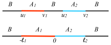
Figure 1: The two configurations of the Ising chain that we consider. Top: the entanglement between two disjoint intervals $A_{1}$ and $A_{2}$ embedded in the ground-state of a larger chain. Bottom: The entanglement between two adjacent intervals in a larger system.

Let us now consider the configuration of two intervals $A_{1}$ and $A_{2}$ of length $\ell_{1}$ and $\ell_{2}$ sharing a common boundary at the origin as graphically depicted in Fig. 1 (bottom). This can be obtained by letting $v_{1}\to u_{2}=0$ in Eq. (9) and it is then described by the 3-point function (we set $u_{1}=-\ell_{1}$ and $v_{2}=\ell_{2}$)

$${\rm Tr}(\rho_{A}^{T_{2}})^{n}=\langle{\cal T}_{n}(-\ell_{1})\overline{\cal T}^{2}_{n}(0){\cal T}_{n}(\ell_{2})\rangle\,,$$ (21)

whose form is determined by global conformal symmetry [27]

$$\langle{\cal T}_{n}(-\ell_{1})\overline{\cal T}^{2}_{n}(0){\cal T}_{n}(\ell_{2})\rangle=\frac{d_{n}}{(\ell_{1}\ell_{2})^{\Delta_{{\cal T}_{n}^{2}}}(\ell_{1}+\ell_{2})^{2\Delta_{{\cal T}_{n}}-\Delta_{{\cal T}_{n}^{2}}}},$$ (22)

where, for simplicity, we have set the UV cutoff $a=1$. Notice that $d_{n}$ is not universal, but can be written as $d_{n}=c_{n}^{2}C_{{\cal T}_{n}\overline{\cal T}^{2}_{n}{\cal T}_{n}}$ where the structure constant $C_{{\cal T}_{n}\overline{\cal T}^{2}_{n}{\cal T}_{n}}$ is universal and can be determined by considering the proper limit of the four-point function as explicitly done in Ref. [25].

For $n=n_{e}$ even, using the dimensions of the twist operators calculated above, we find the universal scaling relation

$${\rm Tr}(\rho_{A}^{T_{2}})^{n_{e}}=\frac{d_{n_{e}}}{(\ell_{1}\ell_{2})^{{c}/6({n_{e}}/2-2/{n_{e}})}(\ell_{1}+\ell_{2})^{{c}/6({n_{e}}/2+1/{n_{e}})}}\,,$$ (23)

that in the limit $n_{e}\to 1$ gives

$$||\rho_{A}^{T_{2}}||\propto\left(\frac{\ell_{1}\ell_{2}}{\ell_{1}+\ell_{2}}\right)^{{c}/4}\qquad\Rightarrow\quad{\cal E}=\frac{c}{4}\ln\frac{\ell_{1}\ell_{2}}{\ell_{1}+\ell_{2}}+{\rm cnst}.$$ (24)

For $n=n_{o}$ odd we have

$${\rm Tr}(\rho_{A}^{T_{2}})^{n_{o}}=\frac{d_{n_{o}}}{(\ell_{1}\ell_{2}(\ell_{1}+\ell_{2}))^{{c}/{12}(n_{o}-{1}/{n_{o}})}},$$ (25)

that for $n_{o}\to 1$ gives ${\rm Tr}\rho_{A}^{T_{2}}=1$ as it should.

2.3 Finite systems.

All previous results are generalized to the case of a finite system of length $L$ with periodic boundary conditions by using a conformal mapping from the cylinder (with axis perpendicular to the spatial coordinate) to the plane. The net effect of the mapping is to replace each length $\ell_{i}$ with the chord length $(L/\pi)\sin(\pi\ell_{i}/L)$ in all above formulas.

Thus for the case of a pure state in a finite system the generalization of Eqs. (16) and (17) are

$${\rm Tr}(\rho_{A}^{T_{2}})^{n_{e}}=c_{n_{e}/2}^{2}\Big{(}\frac{L}{\pi a}\sin\frac{\pi\ell}{L}\Big{)}^{-{c}/{3}({n_{e}}/2-2/{n_{e}})}\,,$$ (26)

$${\rm Tr}(\rho_{A}^{T_{2}})^{n_{o}}=c_{n_{o}}\Big{(}\frac{L}{\pi a}\sin\frac{\pi\ell}{L}\Big{)}^{-{c}/6(n_{o}-1/{n_{o}})}\,,$$ (27)

$${\cal E}=\frac{c}{2}\ln\Big{(}\frac{L}{\pi a}\sin\frac{\pi\ell}{L}\Big{)}+2\ln c_{1/2}\,.$$ (28)

For two adjacent intervals embedded in a finite system, the generalizations of Eqs. (23) and (25) lead to the universal scaling relations

$${\rm Tr}(\rho_{A}^{T_{2}})^{n_{e}}=\frac{d_{n_{e}}}{\left[\frac{L^{2}}{\pi^{2}}\sin\big{(}\frac{\pi\ell_{1}}{L}\big{)}\sin\big{(}\frac{\pi\ell_{2}}{L}\big{)}\right]^{{c}/6({n_{e}}/2-2/{n_{e}})}\left[\frac{L}{\pi}\sin\frac{\pi(\ell_{1}+\ell_{2})}{L}\right]^{{c}/6({n_{e}}/2+1/{n_{e}})}}\,,$$

$${\rm Tr}(\rho_{A}^{T_{2}})^{n_{o}}=\frac{d_{n_{o}}}{\left[\frac{L^{3}}{\pi^{3}}\sin\Big{(}\frac{\pi\ell_{1}}{L}\Big{)}\sin\Big{(}\frac{\pi\ell_{2}}{L}\Big{)}\sin\frac{\pi(\ell_{1}+\ell_{2})}{L}\right]^{{c}/{12}(n_{o}-1/{n_{o}})}},$$ (29)

and for the logarithmic negativity

$${\cal E}=\frac{c}{4}\ln\left[\frac{L}{\pi}\frac{\sin\big{(}\frac{\pi\ell_{1}}{L}\big{)}\sin\big{(}\frac{\pi\ell_{2}}{L}\big{)}}{\sin\frac{\pi(\ell_{1}+\ell_{2})}{L}}\right]+{\rm cnst}.$$ (30)

3 Negativity for two disjoint intervals in the Ising universality class

For a generic CFT with central charge $c$, by using global conformal invariance, the four point function of twist fields can be written as [27, 28]

$$\langle\mathcal{T}_{n}(z_{1})\overline{\cal T}_{n}(z_{2})\mathcal{T}_{n}(z_{3})\overline{\cal T}_{n}(z_{4})\rangle=c_{n}^{2}\left|\frac{z_{31}z_{42}}{z_{21}z_{43}z_{41}z_{32}}\right|^{c/6(n-1/n)}\mathcal{F}_{n}(x,\bar{x})\,,$$ (31)

where the positions $z_{i}\in\mathbb{C}$, $z_{ij}=z_{i}-z_{j}$ and $x$ is the four-point ratio

$$x\equiv\frac{z_{21}z_{43}}{z_{31}z_{42}}\,,$$ (32)

and $\bar{x}$ its complex conjugate. (All distances are measured in units of the UV cutoff $a$.) The function $\mathcal{F}_{n}(x,\bar{x})$ is real and must be computed case by case because it depends on the full operator content of the theory as explicitly done in some CFTs [28, 29, 30, 31, 32, 33, 34, 35] and also numerically in some lattice models [36, 37, 38, 39, 40, 41, 42], but mainly with $x$ real and $0<x<1$. Since $z_{31}z_{42}/(z_{21}z_{43}z_{41}z_{32})=1/(z_{21}z_{43}(1-x))$, the normalization of $\mathcal{F}_{n}(x,\bar{x})$ is given by ${\cal F}_{n}(0,0)=1$. Thus, in the limit $x\to 0$ (i.e. large distance between the two intervals), the four-point function becomes the product of two two-point functions normalized through the constant $c_{n}$.

As explained in Refs. [24, 25], in order to give a physical interpretation to Eq. (31) as ${\rm Tr}\rho_{A}^{n}$ or ${\rm Tr}(\rho_{A}^{T_{2}})^{n}$, the points $z_{i}$ must be on the real axis and their order allows to distinguish between ${\rm Tr}\rho_{A}^{n}$ and ${\rm Tr}(\rho_{A}^{T_{2}})^{n}$. We denote the boundaries of the two intervals with four real variables $u_{j}$ and $v_{j}$ ($j=1,2$) such that $u_{1}<v_{1}<u_{2}<v_{2}$ in both cases. With these definitions, Eq. (31) for ${\rm Tr}\rho_{A}^{n}$ corresponds to $z_{1}=u_{1}$, $z_{2}=v_{1}$, $z_{3}=u_{2}$ and $z_{4}=v_{2}$, leading to

$${\rm Tr}\rho_{A}^{n}=c_{n}^{2}\left(\frac{(u_{2}-u_{1})(v_{2}-v_{1})}{(v_{1}-u_{1})(v_{2}-u_{2})(v_{2}-u_{1})(u_{2}-v_{1})}\right)^{{c}/6(n-1/n)}{\cal F}_{n}(x)\,,$$ (33)

where

$$x=\frac{z_{21}z_{43}}{z_{31}z_{42}}=\frac{(v_{1}-u_{1})(v_{2}-u_{2})}{(u_{2}-u_{1})(v_{2}-v_{1})}\,,$$ (34)

and $0<x<1$. Being $x$ real, the dependence on $\bar{x}=x$ has been dropped.

Instead, ${\rm Tr}(\rho_{A}^{T_{2}})^{n}$ is obtained from the four-point function (31) with the choice $z_{1}=u_{1}$, $z_{2}=v_{1}$, $z_{3}=v_{2}$ and $z_{4}=u_{2}$, namely by exchanging $z_{3}\leftrightarrow z_{4}$ with respect to the previous case. The result can be then written as

$${\rm Tr}(\rho_{A}^{T_{2}})^{n}=c_{n}^{2}\left(\frac{(u_{2}-u_{1})(v_{2}-v_{1})}{(v_{1}-u_{1})(v_{2}-u_{2})(v_{2}-u_{1})(u_{2}-v_{1})}\right)^{{c}/6(n-1/n)}{\cal G}_{n}(y)\,,$$ (35)

with

$$y\equiv\frac{z_{21}z_{34}}{z_{41}z_{32}}=\frac{(v_{1}-u_{1})(v_{2}-u_{2})}{(u_{2}-u_{1})(v_{2}-v_{1})}\,,$$ (36)

and $0<y<1$ and again we dropped the dependence on $\bar{y}$ because $y$ is real. Notice that we have chosen the definitions of $x$ and $y$ in such a way that the functional dependence on $u_{j}$ and $v_{j}$ is the same, but they are two different four-point ratios, as their dependence on $z_{i}$ explicitly shows. The relation between the two is $y=x/(x-1)$. The expressions (33) and (35) are related as

$${\cal G}_{n}(y)=(1-y)^{{c}/3\left(n-{1}/n\right)}\,{\cal F}_{n}\Big{(}\frac{y}{y-1}\Big{)}\,,$$ (37)

as easily derived from Eq. (31).

The logarithmic negativity is obtained by considering the even sequence $n=n_{e}$ and taking its analytic continuation $n_{e}\to 1$. Thus, the functional dependence on $n$ of ${\cal F}_{n}(x)$ for $x=y/(y-1)<0$ must be different for even and odd $n$, in such a way that the limit

$${\cal E}(y)=\lim_{n_{e}\to 1}\ln{\cal G}_{n_{e}}(y)=\lim_{n_{e}\to 1}\ln\left[{\cal F}_{n_{e}}\Big{(}\frac{y}{y-1}\Big{)}\right]\,,$$ (38)

is not trivially equal to $\displaystyle\lim_{n_{o}\to 1}\ln{\cal G}_{n_{o}}(y)=0$. It is natural and convenient to introduce the ratio

$$R_{n}(y)\equiv\frac{\textrm{Tr}(\rho_{A}^{T_{2}})^{n}}{{\rm Tr}\rho_{A}^{n}} = \frac{\langle\mathcal{T}_{n}(u_{1})\overline{\cal T}_{n}(v_{1})\overline{\mathcal{T}}_{n}(u_{2})\mathcal{T}_{n}(v_{2})\rangle}{\langle\mathcal{T}_{n}(u_{1})\overline{\cal T}_{n}(v_{1})\mathcal{T}_{n}(u_{2})\overline{\cal T}_{n}(v_{2})\rangle}$$ (39)

$$= \frac{{\cal G}_{n}(y)}{{\cal F}_{n}(y)}=(1-y)^{c/3(n-1/n)}\,\frac{\mathcal{F}_{n}(y/(y-1))}{\mathcal{F}_{n}(y)}\,.$$

Indeed, in such ratio the prefactors cancel and a function only of $y\in(0,1)$ is left. Moreover, the ratio in Eq. (39) is an easy quantity to consider in the numerical computations. Notice that, being $\displaystyle\lim_{n\to 1}{\rm Tr}\rho_{A}^{n}=1$, the logarithmic negativity is obtained equivalently from the replica limit of this ratio

$${\cal E}(y)=\ln\lim_{n_{e}\to 1}R_{n_{e}}(y)\,.$$ (40)

Thus, while ${\rm Tr}\rho_{A}^{n}$ requires ${\cal F}_{n}(x)$ only for $x\in(0,1)$, in order to extract ${\rm Tr}(\rho_{A}^{T_{2}})^{n}$, and consequently the negativity ${\cal E}(y)$, one has to compute the function ${\cal F}_{n}(x)$ also for $x<0$.

We remark that for the special case $n=2$, we have $\overline{\mathcal{T}}_{2}=\mathcal{T}_{2}$ because $\mathcal{T}_{2}^{2}$ is the identity operator. This implies that $R_{2}(y)=1$ for $0<y<1$ identically.

In order to find $\mathcal{F}_{n}(x,\bar{x})$ for the Ising model, it is useful to review the corresponding result for the free compactified boson (i.e. a Luttinger liquid field theory), derived in Ref. [25].

3.1 Free compactified boson

For the free real boson compactified on a circle of radius $R$, the function $\mathcal{F}_{n}(x,\bar{x})$ in Eq. (31) for any complex $x$ has been computed in [25]. This has been possible starting from some results in Refs. [43, 44] and generalizing to $x\in\mathbb{C}$ the procedure employed in Ref. [29] for $0<x<1$. The final result is [25]

$$\mathcal{F}_{n}(x,\bar{x})=\frac{\Theta\big{(}{\bf 0}|T_{\eta}(x,\bar{x})\big{)}}{\prod_{k=1}^{n-1}|F_{k/n}(x)|}\,,$$ (41)

where we introduced $F_{k/n}(x)\equiv\,_{2}F_{1}(k/n,1-k/n;1;x)$ to denote the special case of the hypergeometric function ${}_{2}F_{1}(a,b;c;z)$. Here $\Theta({\bf 0}|K)$ is of the Riemann-Siegel theta function which is generically defined as

$$\Theta({\bf 0}|K)\,\equiv\,\sum_{{\bf m}\,\in\,\mathbf{Z}^{p}}\exp\big{[}i\pi\,{\bf m}\cdot K\cdot{\bf m}\big{]}\,,$$ (42)

where $K$ is a $p\times p$ symmetric complex matrix with positive definite imaginary part and ${\bf 0}$ is the $p$ dimensional vector made by zeros. The $2(n-1)\times 2(n-1)$ symmetric complex matrix $T_{\eta}(x,\bar{x})$ entering in Eq. (41) is

$$T_{\eta}(x,\bar{x})=\left(\begin{array}[]{cc}i\eta\mathcal{I}&\mathcal{R}\\ \mathcal{R}&i\mathcal{I}/\eta\end{array}\right)\,,$$ (43)

where the parameter $\eta$ is proportional to $R^{2}$ and the $(n-1)\times(n-1)$ symmetric real matrices $\mathcal{R}$ and $\mathcal{I}$ are respectively the real and the imaginary part of the $(n-1)\times(n-1)$ period matrix

$$\tau(x)=\mathcal{R}+i\,\mathcal{I}=\frac{2}{n}\sum_{k=1}^{n-1}\tau_{k/n}(x)\sin(\pi k/n)\,C_{k/n}\,,$$ (44)

with

$$\tau_{k/n}(x)\equiv i\,\frac{F_{k/n}(1-x)}{F_{k/n}(x)}\,,$$ (45)

and $C_{k/n}$ is the $(n-1)\times(n-1)$ symmetric matrix whose elements read

$$\big{(}C_{k/n}\big{)}_{rs}=\cos\big{[}2\pi k/n(r-s)\big{]}\,,\hskip 28.45274ptr,s=1,\dots,n-1\,.$$ (46)

Notice that, because of the $k\leftrightarrow n-k$ invariance of the functions $F_{k/n}$, for $n$ odd the denominator in (41) becomes the square of a product over $k$ going from 1 to $(n_{o}-1)/2$. Similarly, (44) can be written as a sum over $k$ going from 1 to $(n_{o}-1)/2$. This suggests that the term corresponding to $k/n=1/2$, occurring only for even $n$, plays a key role in the limit (38), as shown explicitly in [25] for the non-compactified boson in the limit of close intervals.

Few comments are now in order regarding Eq. (41) before proceeding to the partial transpose. Comparing Eq. (41) with old results about CFT on higher genus Riemann surfaces [44, 45, 46, 47, 48], one observes that $\mathcal{F}_{n}(x,\bar{x})$ is related to the partition function $\mathcal{Z}=\mathcal{Z}^{\rm qu}\mathcal{Z}^{\rm cl}(R)$ on a genus $g=n-1$ Riemann surface, which can be factorized into a quantum part and a classical part, and all the dependence on $R$ of $\mathcal{Z}$ is contained in the latter. In particular, one finds that $\mathcal{Z}^{\rm cl}(R)=\Theta({\bf 0}|T_{\eta}(x,\bar{x}))$ and the period matrix of the Riemann surface is $\tau(x)$ given in (44). As already remarked [43, 29], here we are not dealing with generic genus $g$ Riemann surfaces, but with a subclass of them obtained through the replica method (see the appendix of [30] for a pictorial representation). Thus, while for ${\rm Tr}\rho_{A}^{n}$ one needs the period matrix $\tau(x)$ only for $0<x<1$, where its real part $\mathcal{R}$ vanishes identically, for ${\rm Tr}(\rho_{A}^{T_{2}})^{n}$ the period matrix $\tau(x)$ for $x<0$ is required and in this regime $\mathcal{R}$ enters in a crucial way. The expression (41) is explicitly invariant under $\eta\leftrightarrow 1/\eta$. We recall that one can also rewrite Eq. (41) in a form which makes manifest its invariance under $x\leftrightarrow 1-x$. This form is particularly useful also to study the regime $\eta\to\infty$ of non-compactified boson because some simplifications occur and the Riemann-Siegel theta function does not contribute in this limit [25].

At this point, it is easy to write ${\rm Tr}(\rho_{A}^{T_{2}})^{n}$ for the compactified boson from Eq. (35), where ${\cal G}_{n}(y)$ is given by (37) with $c=1$ and ${\cal F}_{n}(x)$ by (41), i.e.

$${\cal G}_{n}(y)=(1-y)^{(n-1/n)/3}\,\frac{\Theta\big{(}{\bf 0}|T_{\eta}(\frac{y}{y-1})\big{)}}{\prod_{k=1}^{n-1}\big{|}F_{k/n}(\frac{y}{y-1})\big{|}}\,,$$ (47)

where $0<y<1$. From Eqs. (47) and (41), we can write the ratio (39) for the free compactified boson

$$R_{n}(y)=(1-y)^{(n-1/n)/3}\left(\,\prod_{k=1}^{n-1}\bigg{|}\frac{F_{k/n}(y)}{F_{k/n}(\frac{y}{y-1})}\bigg{|}\,\right)\frac{\Theta\big{(}{\bf 0}|T_{\eta}(\frac{y}{y-1})\big{)}}{\Theta\big{(}{\bf 0}|T_{\eta}(y)\big{)}}\,.$$ (48)

In the decompactification regime $\eta\to\infty$, this formula has been checked numerically in Ref. [25] for an harmonic chain with periodic boundary conditions, whose Hamiltonian is the lattice discretization of a free boson (Klein-Gordon action). Always in this regime and in the limit $y\rightarrow 1^{-}$ of close intervals, the analytic continuation $n_{e}\to 1$ of the even sequence $R_{n_{e}}(y)$ has been explicitly carried out [25]. The analytic continuation $n_{e}\rightarrow 1$ for finite and generic $\eta$ is still unknown. A similar problem occurs for the von Neumann entanglement entropy through the analytic continuation of the Rényi entropies of two disjoint intervals. We finally mention that the results for some finite $\eta$ have been recently checked in Monte Carlo simulations [50].

3.2 Ising conformal field theory

In the previous section we have shown that ${\cal F}_{n}(x,\bar{x})$ can be found from the partition function of the corresponding model on the genus $g=n-1$ Riemann surface obtained from the replica method. The partition function of the Ising model on a genus $g$ Riemann surface has been derived in the eighties [45, 46, 48, 49] by considering $\mathbb{Z}_{2}$ orbifolds models on generic Riemann surfaces. From the knowledge of the partition function $\mathcal{Z}=\mathcal{Z}^{\rm qu}\mathcal{Z}^{\rm cl}(R)$ of the compactified boson on the same Riemann surface, we can explicitly access the period matrix on the Riemann surface. Then, using the mentioned old results for the Ising model on a genus $g$ Riemann surface, we can finally write [30]

$$\mathcal{Z}_{\rm Ising}=(\mathcal{Z}^{\rm qu})^{1/2}\,2^{-g}\sum_{{\bf e}}\big{|}\Theta[{\bf e}]\big{(}{\bf 0}|\tau\big{)}\big{|}\,,$$ (49)

where $\tau$ is the $g\times g$ period matrix. Here we introduced the Riemann-Siegel theta function with characteristic ${\bf e}$, which is defined as

$$\Theta[{\bf e}]({\bf z}|\tau)=\sum_{{\bf m}\,\in\,\mathbb{Z}^{g}}e^{i\pi\big{[}({\bf m}+\bm{\varepsilon})\cdot\tau\cdot({\bf m}+\bm{\varepsilon})+2({\bf m}+\bm{\varepsilon})\cdot({\bf z}+\bm{\delta})\big{]}}\,,$$ (50)

where ${\bf z}\in\mathbb{C}^{g}/(\mathbb{Z}^{g}+\tau\,\mathbb{Z}^{g})$ is a $g$ dimensional complex vector and the characteristic ${\bf e}$ is given by a pair of $g$ dimensional vectors $\bm{\varepsilon}$ and $\bm{\delta}$ made by $0$’s and $1/2$’s

$$[{\bf e}]=\bigg{[}\begin{array}[]{c}\bm{\varepsilon}\\ \bm{\delta}\end{array}\bigg{]}=\bigg{[}\begin{array}[]{c}\varepsilon_{1},\dots,\varepsilon_{g}\\ \delta_{1},\dots,\delta_{g}\end{array}\bigg{]}\,,\hskip 45.52458pt\varepsilon_{i},\delta_{i}\in\{0,1/2\}\,.$$ (51)

In the case at hand, the period matrix $\tau(x)$ is given by Eq. (44) and the partition function for the compactified boson $\mathcal{Z}=\mathcal{Z}^{\rm qu}\mathcal{Z}^{\rm cl}(R)$ is Eq. (41). Thus, for the Ising model we have

$$\mathcal{F}_{n}(x,\bar{x})=\frac{\sum_{{\bf e}}\big{|}\Theta[{\bf e}]\big{(}{\bf 0}|\tau(x)\big{)}\big{|}}{2^{n-1}\prod_{k=1}^{n-1}\big{|}F_{k/n}(x)\big{|}^{1/2}}\,.$$ (52)

For $0<x<1$, this function reduces to $\mathcal{F}_{n}(x)$ found in [30] for the Rényi entropies of the Ising model and it has been tested numerically through various methods [38, 39, 40], finding agreement once the finite size corrections are properly taken into account.

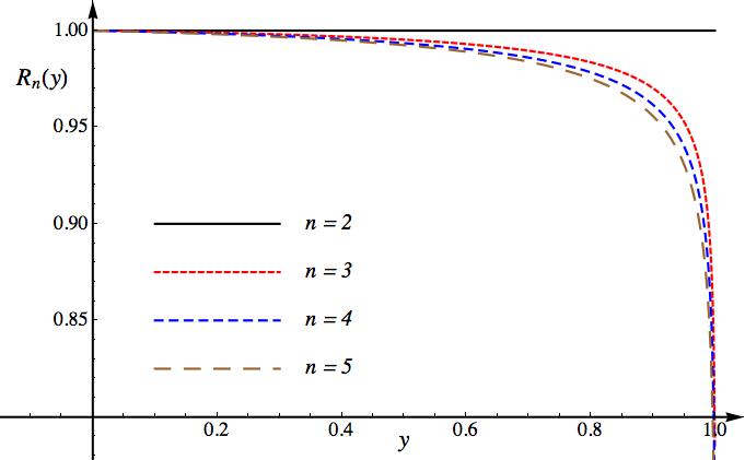
Figure 2: The function $R_{n}(y)$ for the Ising conformal field theory as a function of $y$ for several values of $n$ ($n=2,3,4,5$ curves from top to bottom).

Writing ${\rm Tr}(\rho_{A}^{T_{2}})^{n}$ for the Ising model is now easy by using Eq. (35) with $c=1/2$, and ${\cal G}_{n}(y)$ from Eqs. (37) and (52), namely

$${\cal G}_{n}(y)=(1-y)^{(n-1/n)/6}\,\frac{\sum_{{\bf e}}\big{|}\Theta[{\bf e}]\big{(}{\bf 0}|\tau(\frac{y}{y-1})\big{)}\big{|}}{2^{n-1}\prod_{k=1}^{n-1}\big{|}F_{k/n}(\frac{y}{y-1})\big{|}^{1/2}}\,,$$ (53)

where $0<y<1$ and $\tau$ is given by Eq. (44). From this expression and Eq. (52), we can write the ratio (39) for the Ising model

$$R_{n}(y)=(1-y)^{(n-1/n)/6}\,\prod_{k=1}^{n-1}\bigg{|}\frac{F_{k/n}(y)}{F_{k/n}(\frac{y}{y-1})}\bigg{|}^{{1}/{2}}\,\frac{\sum_{{\bf e}}\big{|}\Theta[{\bf e}]\big{(}{\bf 0}|\tau(\frac{y}{y-1})\big{)}\big{|}}{\sum_{{\bf e}}\big{|}\Theta[{\bf e}]\big{(}{\bf 0}|\tau(y)\big{)}\big{|}}\,.$$ (54)

The curves $R_{n}(y)$ for $0<y<1$ are shown in Fig. 2 for $n=2,3,4,5$. They are concave curves with $R_{n}(0)=1$, which stay below 1 for $n>2$. When $n=2$, we have $R_{2}(y)=1$ identically, as we will explicitly prove below. Moreover, $R_{n_{2}}(y)<R_{n_{1}}(y)$ when $n_{2}>n_{1}$, for all $0<y<1$. Approaching $y=1$, $R_{n}(y)$ approaches zero very steeply in a calculable power-law way that, for a general model, depends only on the central charge [25].

It is worth mentioning that after a superficial analysis, one could erroneously conclude that the sum over the characteristics occurring in Eq. (52) involves $2^{2g}$ terms. This is not true because many of these terms are identically zero. In order to see this, let us introduce the parity of the characteristic ${\bf e}$ which is the parity of the integer number $4\bm{\varepsilon}\cdot\bm{\delta}$ which is related to the transformation property of the Riemann-Siegel theta function [46]

$$\Theta[{\bf e}](-{\bf z}|\tau)=(-1)^{4\bm{\varepsilon}\cdot\bm{\delta}}\Theta[{\bf e}]({\bf z}|\tau)\,.$$ (55)

There are $2^{g-1}(2^{g}+1)$ even characteristics and $2^{g-1}(2^{g}-1)$ odd ones. Eq. (55) implies that $\Theta[{\bf e}]({\bf 0}|\tau)=0$ identically for odd characteristics. This means that the sum over the characteristics which defines $\mathcal{F}_{n}(x,\bar{x})$ in (52) is made only by $2^{n-2}(2^{n-1}+1)$ terms, namely the ones with even ${\bf e}$.

3.3 The special case $n=2$ for Ising model.

For the special case of $n=2$, since $\mathcal{T}_{2}=\overline{\cal T}_{2}$, we have $R_{2}(y)=1$ identically in $0<y<1$. This is true for any CFT, as already noted above, and therefore also for the Ising model. Nevertheless, we find it instructive to see explicitly how this simplification occurs in Eq. (54), since this is not apparent from the formula and the explicit proof is related to the modular invariance of the torus partition function [51].

When $n=2$ the Riemann surface is a torus and the period matrix reduces to its modulus $\tau(x)=\tau_{1/2}(x)$, which is a complex number. In this case the four-point ratio $x\in\mathbb{C}$ and its modulus $\tau(x)$ are related as [43, 28]

$$F_{1/2}(x)=\frac{2}{\pi}K(x)=\theta_{3}(\tau(x))^{2},\qquad\tau(x)=\frac{iK(1-x)}{K(x)},\qquad x(\tau)=\left(\frac{\theta_{2}(\tau)}{\theta_{3}(\tau)}\right)^{4},$$ (56)

where $K(x)$ is the complete elliptic integral of the first kind. From the properties of $K$, for $0<y<1$ one finds [52]

$$F_{1/2}\left(\frac{1}{1-y}\right) = \frac{2}{\pi}\sqrt{1-y}\big{(}K(1-y)-iK(y)\big{)}\,,$$ (57)

$$\rule{0.0pt}{18.49411pt}F_{1/2}\left(\frac{y}{y-1}\right) = \frac{2}{\pi}\sqrt{1-y}\,K(y)\,.$$ (58)

Given $\tau=\tau(y)$ in the second formula of (56), (57) and (58), it is straightforward to observe that for $0<y<1$ we have

$$\tau^{\prime}\equiv\tau\left(\frac{y}{y-1}\right)=\tau+1\,.$$ (59)

We also need to recall the following transformation properties of the Jacobi theta functions under the modular transformation $\tau\rightarrow\tau+1$ [27, 51]

$$\theta_{2}(\tau+1)=e^{i\pi/4}\theta_{2}(\tau)\,,\hskip 34.14322pt\theta_{3}(\tau+1)=\theta_{4}(\tau)\,,\hskip 34.14322pt\theta_{4}(\tau+1)=\theta_{3}(\tau)\,.$$ (60)

From the first formula in (56), (59) and the second formula in (60), one finds that

$$F_{1/2}\left(\frac{y}{y-1}\right)=\theta_{3}(\tau+1)^{2}=\theta_{4}(\tau)^{2}\,.$$ (61)

Given the expressions above, we are ready to prove that $R_{2}(y)=1$ for $0<y<1$. Indeed, from Eqs. (56) and (61) we get

$$(1-y)^{1/4}=\left|\frac{\theta_{4}(\tau)}{\theta_{3}(\tau)}\right|\,,\qquad\bigg{|}\frac{F_{1/2}(y)}{F_{1/2}(\frac{y}{y-1})}\bigg{|}^{1/2}=\left|\frac{\theta_{3}(\tau)}{\theta_{4}(\tau)}\right|\,,$$ (62)

where in the first equation the identity $\theta^{4}_{4}=\theta^{4}_{3}-\theta^{4}_{2}$ has been employed. As for the ratio containing the Riemann-Siegel theta functions in (54), when $n=2$ and $0<y<1$, it simplifies to

$$\frac{|\theta_{2}(\tau^{\prime})|+|\theta_{3}(\tau^{\prime})|+|\theta_{4}(\tau^{\prime})|}{|\theta_{2}(\tau)|+|\theta_{3}(\tau)|+|\theta_{4}(\tau)|}=1\,,$$ (63)

where Eq. (59) and the modular transformations (60) have been employed.

4 The partial transposition with Tree Tensor Networks

The Ising chain in a transverse magnetic field is the most studied one dimensional model and this is mainly due to fact that it is a non-trivial model that can be mapped to a system of free fermions by means of a Jordan-Wigner transformation [53]. However, it is still a very hard problem to find an effective way to calculate the partial transpose of the reduced density matrix (or at least its eigenvalues) in the free fermions formulation as opposite to models of free bosons for which many results are already available (see e.g. [14, 16, 25]). For this reason, in order to check the analytical predictions from conformal field theory, we resort to purely numerical methods based on tree tensor techniques which already have been very effective in calculating of the entanglement entropies of two disjoint intervals [38, 40]. An alternative approach based on classical Monte Carlo simulations (generalizing the method in Refs. [54, 38, 40, 55]) has been also independently developed at the same time of this work by V. Alba [50].

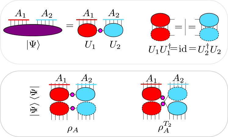
Figure 3: Graphical representations of some quantities for a pure state and of some useful properties in the language of the tensor networks. Top: We consider the bipartition of the pure state $|\Psi\rangle$ in $A_{1}$ and $A_{2}$ and its Schmidt decomposition through the isometries $U_{1}$ and $U_{2}$. Bottom left: the density matrix $\rho_{A}$. Bottom right: the partial transpose $\rho_{A}^{T_{2}}$.

4.1 Tensor networks: notation and examples

We consider a 1D lattice $\mathcal{L}$ made of $L$ sites and on each site $s\in\mathcal{L}$ we set a local Hilbert space $\mathbb{V}_{s}$ of finite dimension $d$ (e.g. for a spin-$1/2$ for which $d=2$). An arbitrary pure state $\ket{\Psi}\in\mathbb{V}^{\otimes L}$ defined on the lattice $\mathcal{L}$, in the local basis $\{\ket{1_{s}},\ket{2_{s}},\cdots,\ket{d_{s}}\}$ of $\mathbb{V}_{s}$, can be expanded as follows

$$|\Psi\rangle=\!\sum_{i_{1}=1}^{d}~{}\sum_{i_{2}=1}^{d}\cdots\sum_{i_{L}=1}^{d}T_{i_{1}i_{2}\cdots i_{L}}\ket{i_{1}}\ket{i_{2}}\cdots\ket{i_{L}},$$ (64)

i.e. can be encoded in a tensor $T$ whose $d^{L}$ elements $T_{i_{1}i_{2}\cdots i_{L}}\in\mathbb{C}$ fully determine the state. We refer to the index $1\leqslant i_{s}\leqslant d$, labeling a local basis for site $s$, as a physical index.

The tensor network approach [56] is a powerful way to rewrite the exponentially large tensor $T$ in Eq. (64) as a combination of smaller tensors. However, the manipulations required to make the products of these tensors easily become too long and cumbersome to write explicitly all indices and then it is very convenient to represent them by diagrams. In these diagrams each tensor is represented by circles having some outgoing lines and each of them represents a tensor’s index. For each tensor, we denote its complex conjugate with the same circle delimitated by a dashed line instead of a continuos one. A line shared by two tensors represents a contraction of a particular index.

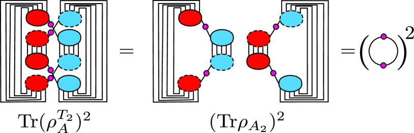
Figure 4: Graphical representation of the identity ${\rm Tr}(\rho_{A}^{T_{2}})^{n_{e}}=({\rm Tr}\rho_{A_{2}}^{n_{e}/2})^{2}$ for $n_{e}=2$.

In order to show the power and simplicity of this diagrammatic representation in a concrete example, we will graphically prove the identities ${\rm Tr}(\rho_{A}^{T_{2}})^{n_{e}}=({\rm Tr}\rho_{A_{2}}^{n_{e}/2})^{2}$ and ${\rm Tr}(\rho_{A}^{T_{2}})^{n_{o}}={\rm Tr}\rho_{A_{2}}^{n_{o}}$ [25], which hold when $B=\emptyset$ and the whole chain $A=A_{1}\cup A_{2}$ is in a pure state. Let us consider the case of a chain $A$ made by $8$ spins and a bipartition such that both $A_{1}$ and $A_{2}$ contain $4$ spins (but the validity of the proof does not rely on these numbers). The pure state $|\Psi\rangle$ is depicted in the top of Fig. 3 where also its Schmidt decomposition is shown (the different colors of the circles refer to $A_{1}$ and $A_{2}$). The small (purple) circle on the line connecting the two big circles stands for the diagonal matrix formed by the Schmidt coefficients $c_{\alpha}$, i.e. $|\Psi\rangle=\sum_{\alpha}c_{\alpha}|e^{(1)}_{\alpha}\rangle\otimes|e^{(2)}_{\alpha}\rangle$. We recall that the Schmidt vectors $|e^{(1)}_{\alpha}\rangle$ and $|e^{(2)}_{\alpha}\rangle$ provide an orthonormal basis and this ensures that the transformation matrices $U_{1}$ and $U_{2}$ are isometric [57], a property that graphically can be depicted as in Fig. 3 (top right). The density matrix $\rho_{A}=|\Psi\rangle\langle\Psi|$ is given by the picture on the bottom (left part) of Fig. 3. The definition of $\rho_{A}^{T_{2}}$ given in Eq. (3) can be implemented in the tensor network language by interchanging the tensor associated to $A_{2}$ and its complex conjugate, as again shown in Fig. 3 (bottom right).

Now we are ready to show how the above identities for pure states can be easily proved by using the graphical representation. We first consider even powers, i.e. ${\rm Tr}(\rho_{A}^{T_{2}})^{n_{e}}=({\rm Tr}\rho_{A_{2}}^{n_{e}/2})^{2}$. In Fig. 4, for sake of graphical simplicity, we restrict to $n_{e}=2$ (which trivially gives $1$ because of the normalization condition ${\rm Tr}\rho_{A_{2}}=1$) but the key steps hold for any even $n_{e}$. ${\rm Tr}(\rho_{A}^{T_{2}})^{2}$ is obtained by contracting the indices of two copies of $\rho_{A}^{T_{2}}$ as shown in Fig. 4 (left), and then realizing that the result factorizes into the product of two ${\rm Tr}\rho_{A_{2}}$ as in the middle of Fig. 4. Using the isometry property in Fig. 3, each ${\rm Tr}\rho_{A_{2}}$ further reduces to the sum of the squared Schmidt coefficients, as it should. ${\rm Tr}(\rho_{A}^{T_{2}})^{n_{o}}$ is graphically calculated in Fig. 5 for $n_{o}=3$. As above, we first write ${\rm Tr}(\rho_{A}^{T_{2}})^{3}$ through the proper contractions of three copies of $\rho_{A}^{T_{2}}$. Then, by rearranging the order of the tensors, this can be put as in the center of Fig. 5, which is ${\rm Tr}\rho_{A_{2}}^{3}$. Again, the last step can be obtained through the isometry property in Fig. 3. These two examples make manifest the power of the graphical notation. Finally, it is worth stressing, that the same proof could have been done in any other basis. We choose the Schmidt one only because in this basis the reduced density $\rho_{A_{2}}$ matrix is diagonal.

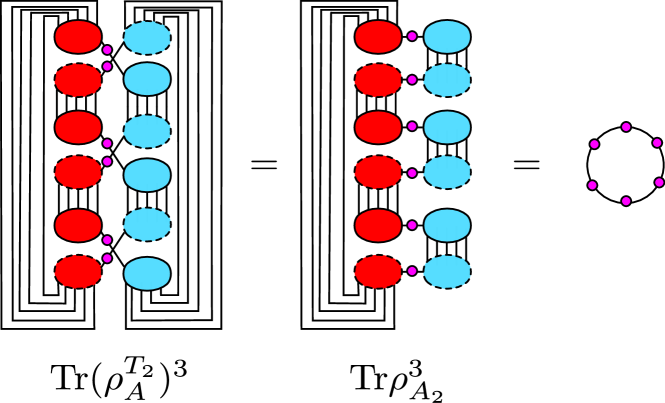
Figure 5: Graphical representation of the identity ${\rm Tr}(\rho_{A}^{T_{2}})^{n_{o}}={\rm Tr}\rho_{A_{2}}^{n_{o}}$ for $n_{o}=3$.

4.2 The Tree Tensor Network

Hereafter we focus on the specific tensor network that we have used for the calculation of the partially transposed reduced density matrix, i.e. the Tree Tensor Networks (TTN). We only briefly recall the basics of the method and for a more detailed explanation, we refer the reader to Refs. [55, 56, 57, 58, 59, 60, 61, 62, 63, 64, 65, 66, 67, 68].

Representing the pure state $|\Psi\rangle$ as in Eq. (64) with a TTN implies that the $d^{L}$ coefficients of the tensor $T_{i_{1}i_{2}\cdots i_{L}}$ can be obtained as the result of the contraction of a network made by tensors $w$ (built with a smaller number of indices) forming a pattern whose shape reminds a tree structure, as graphically shown in Fig. 6 for a lattice of $L=16$ sites and tensors $w$ which have three indices. The TTN decomposition of $T_{i_{1}i_{2}\cdots i_{L}}$ is given by a collection of tensors $w$, hierarchically organized in layers labelled by $\tau$, with $\tau=0,\dots,N$ and $(N+1)=\log_{2}L$. The tensors $w$ have both bond indices and physical indices. All the bond indices are contracted while the $L$ physical indices are left non contracted, so that they can be thought as the leaves of the tree. In this way, the TTN encodes the $d^{L}$ complex coefficients $T_{i_{1}i_{2}\cdots i_{L}}$ of the state in Eq. (64).

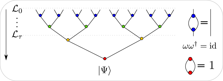
Figure 6: A state $|\Psi\rangle$ encoded by a tree tensor network involving 16 spins.

In the example of Fig. 6, each elementary tensor $w$ has at most one lower index (leg) $\alpha$ and two upper indices (legs) $\beta_{1}$ and $\beta_{2}$ and for this reason is called a binary tree, which is the only structure we will consider. At each level $\tau$, we allow the indices $\beta_{i}$ to run from $1$ to $\chi_{\tau}$. Without loss of generality, the tensor $w$ can be chosen to be isometric [57], i.e. $\omega\omega^{\dagger}=\textrm{id}_{\chi}$, with $\textrm{id}_{\chi}$ being the $\chi\times\chi$ identity tensor. Explicitly, this condition reads

$$\sum_{\beta_{1},\beta_{2}=1}^{\chi_{\tau}}(w)^{\beta_{1}\beta_{2}}_{\alpha}(w^{\dagger})_{\beta_{1}\beta_{2}}^{\alpha^{\prime}}=\delta_{\alpha\alpha^{\prime}}\,,\hskip 28.45274pt\tau=0,\dots,N-1\,,\hskip 14.22636pt\alpha,\alpha^{\prime}=1,\dots,\chi_{\tau+1}\,.$$ (65)

The bottommost tensor of the network (the red one in Fig. 6), i.e. the only tensor at the layer $N$, is different from the others. Indeed, since it does not possess any lower index, it represents a normalized vector, namely

$$\sum_{\beta_{1},\beta_{2}}(w)^{\beta_{1}\beta_{2}}(w^{\dagger})_{\beta_{1}\beta_{2}}=1\,,\hskip 42.67912pt\tau=N\,.$$ (66)

The properties (65) and (66), which are graphically shown on the right of Fig. 6, guarantee that the state $|\Psi\rangle$ in (64) is normalized to 1, i.e. $\braket{\Psi}{\Psi}=1$. These considerations can be generalized to cases with elementary tensors having more upper and lower legs [58]. The natural layered structure of the TTN is emphasized by the arrow on the left of Fig. 6. Each layer is an isometric transformation that maps a lattice $\mathcal{L}_{\tau}$ consisting of $L_{\tau}$ sites to a lattice $\mathcal{L}_{\tau+1}$ with $L_{\tau+1}=L_{\tau}/2$ sites. The physical lattice is $\mathcal{L}_{0}$, whose length $L_{0}=L$ must be a power of $2$. The arrow on the left of Fig. 6 shows the direction along which the coarse-graining of the lattice increases.

In order to describe the ground state of a local Hamiltonian $H$, the tensors of the network should describe the state $|\Psi\rangle$ that minimizes $\langle\Psi|H|\Psi\rangle$. This can be achieved using the (numerical) algorithm described in Ref. [58] whose computational cost is $\chi_{max}^{4}$, where $\chi_{max}=\textrm{max}_{\tau}\{\chi_{\tau}\}$ is the largest bond dimension in the network. Recently, the TTN has been combined with Monte Carlo sampling obtaining an algorithm whose cost scales with $\chi_{max}^{3}$ [70]. Each layer of the TTN encoding the ground state of $H$ is a coarse-graining transformation that selects those states of $\mathcal{L}_{\tau}$ which are relevant for the low energy physics of $H$ at the scale of $\mathcal{L}_{\tau+1}$. When both the Hamiltonian and its ground state are translational invariant, we can force the coarse graining transformations to map translational invariant states on $\mathcal{L}_{\tau}$ into translational invariant states on $\mathcal{L}_{\tau+1}$ by choosing the elementary isometries of the layer $\tau$ to be all equal. This is represented by the color scheme adopted in Fig. 6, where all the isometries belonging to the same layer have the same color.

4.3 Computing the reduced density matrix

Here we briefly describe how to compute the spectrum of the reduced density matrix $\rho_{A}$ of a subsystem $A$ in a given spin chain [58, 40]. To this aim we should first notice that even when the state $|\Psi\rangle$ is translational invariant, by construction the TTN does not enjoy this symmetry. As a consequence, there are choices of the subsystem $A$ for which the computation of the spectrum of $\rho_{A}$ is simpler. This happens when $A$ is chosen to be one block (or several blocks $A_{i}$) of spins of the original lattice which are coarse grained by the TTN to a single spin at some level $\tilde{\tau}<N$. For example, given the structure in Fig. 6, it is easier to compute the spectrum of $\rho_{A}$ made by two spins when they belong to the same isometry, since they are coarse grained to a single spin in one layer. This is due to the fact that, in order to compute the spectrum of $\rho_{A}$, we do not need to build the full matrix $\rho_{A}$, but only a simplified matrix $\tilde{\rho}_{A}$ which is related to $\rho_{A}$ by similarity transformation, i.e.

$$\rho_{A}\equiv\Omega_{A}\,\tilde{\rho}_{A}\,\Omega_{A}^{\dagger}\,.$$ (67)

The matrix $\Omega_{A}$ corresponds to the contraction of all the isometries $\omega$ involved in this coarse-graining process and it transforms each original block $A_{i}$ into a single spin (see Fig. 7). The matrices $\tilde{\rho}_{A}$ are $\chi_{\tilde{\tau}}^{m}\times\chi_{\tilde{\tau}}^{m}$, being $\chi_{\tilde{\tau}}$ the dimensions of the open bonds in $\tilde{\rho}_{A}$ and $m$ is the numbers of disjoint intervals composing $A$ (in this paper we will limit have to $m=1$ and $m=2$). Although $\tilde{\rho}_{A}$ and $\rho_{A}$ have different dimensions (with $\tilde{\rho}_{A}$ smaller than $\rho_{A}$), they have the same spectrum, because they are related by isometries.

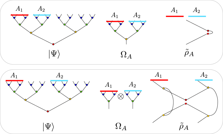
Figure 7: Quantities involved in the computation of the $\rho_{A}$ through a TTN algorithm. Top: $A$ is made by two adjacent intervals. Bottom: $A$ is made by two disjoint intervals.

Thus, we can focus on the computation of $\tilde{\rho}_{A}$. In this process, we can identify three groups of tensors: (i) the tensors whose support is fully contained in $B$; (ii) the tensors whose support is fully contained in $A$; (iii) the tensors whose support is shared between $A$ and its complement. The tensors (i) disappear from the calculation because they are contracted through Eq. (65). The tensors (ii) just define $\Omega_{A}$ and therefore they do not occur in the computation of $\tilde{\rho}_{A}$. Thus, only the tensors of type (iii) are needed for the computation of $\tilde{\rho}_{A}$ which is achieved by contracting these tensors as shown in Fig. 7. Once the simplified tensor network encoding $\tilde{\rho_{A}}$ has been contracted, its diagonalization provides the spectrum of $\rho_{A}$. The upper bound of the computational cost of the whole algorithm is $\chi_{max}^{6}$.

Different block configurations (e.g. not optimal choices of $A_{1}$ and $A_{2}$ or odd $A_{i}$ made by odd number of spins) can also be obtained from the TTN. Naively, one could think that this requires a higher computational cost, but, with some efforts, it is possible to envisage more complicated computational strategies to reduce the cost to $\chi_{max}^{6}$, as discussed in Ref. [69] in a different context.

4.4 Computing the partial transpose

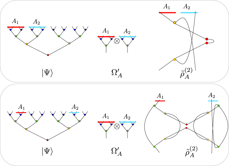
Figure 8: Quantities involved in the computation of the $\rho_{A}^{T_{2}}$ through a TTN algorithm. Top: $A$ is made by two adjacent intervals. Bottom: $A$ is made by two disjoint intervals.

The calculation of the spectrum of the partial transpose of $\rho^{T_{2}}_{A}$ is very similar to the one explained above for the spectrum of $\rho_{A}$. First we have to choose $A$ as above, namely such that each $A_{i}$ becomes a single spin at level $\tilde{\tau}$. Then, we can identify three groups of tensors : (I) the tensors fully contained into $B$; (II) the tensors fully contained into either $A_{1}$ or $A_{2}$ (not both); (III) the tensors connecting $A_{1}$ and $A_{2}$ or $A_{i}$ and $B$. Notice that, while (I) is the same as (i) above, the group (II) is different from (ii) and, consequently, also (III) is not (iii). Let us focus on computing

$$\rho_{A}^{T_{2}}\equiv{\Omega^{\prime}}_{A}\,\tilde{\rho}^{(2)}_{A}\,{\Omega^{\prime}}_{A}^{\dagger},$$ (68)

where ${\Omega^{\prime}}_{A}$ is an isometric tensor (i.e. ${\Omega^{\prime}}_{A}{\Omega^{\prime}}_{A}^{\dagger}=\textrm{id}_{\chi_{\tilde{\tau}}^{m}}$). For the same reasons discussed in the subsection 4.3, only the tensor of type (III) enter in the definition of $\tilde{\rho}^{(2)}_{A}$.

When $A$ is made by two disjoint blocks (see Fig. 8, bottom panel), the matrix $\tilde{\rho}^{(2)}_{A}$ is given by $\tilde{\rho}^{(2)}_{A}=\tilde{\rho}_{A}^{T_{2}}$. For two adjacent blocks (see Fig. 8, top panel) this relation does not hold because $\tilde{\rho}_{A}$ has only one incoming and one outgoing bond and therefore we cannot distinguish between $A_{1}$ and $A_{2}$, which is necessary in order to perform the partial transposition. In this case, indeed we have ${\Omega^{\prime}}_{A}\neq{\Omega}_{A}$ and the former reads

$${\Omega^{\prime}}_{A}=\Omega_{A_{1}}\otimes\Omega_{A_{2}}.$$ (69)

Comparing the top panel of Fig. 8 (center) to the top panel of Fig. 7 (center), we realize that the yellow isometry connecting $A_{1}$ to $A_{2}$ does not occur in ${\Omega^{\prime}}_{A}$, in contrast with ${\Omega}_{A}$. Indeed, the yellow isometry appears in $\tilde{\rho}^{(2)}_{A}$. We finally mention that the computational cost of all the algorithm to determine the spectrum of $\rho_{A}^{T_{2}}$ is upper-bounded by $\chi_{max}^{6}$.

5 Numerical results for the critical Ising chain in a transverse magnetic field

In this section we report numerical results for the transverse field Ising chain obtained by means of the tree tensor network as explained in the previous section. We consider chains of finite length $L$ of the form $L=2^{M}$ and the maximum size studied is $L=512$. The $\chi_{max}$ for this simulation has been fixed to $128$, guaranteeing a relative precision on the ground state energy of about $10^{-8}$. We recall that with the TTN method, using a binary tree, we can quickly access only subsystems of size $\ell=2^{m}$ with $m<M$ integer, as it should be clear from the previous section.

As a first calculation we considered a bipartite chain (i.e. $B\to\emptyset$) and we checked that the entanglement negativity reproduces the Rényi entropy $S^{(1/2)}_{A_{2}}$, as it should. We do not report explicit plots of these results, but they have been important numerical checks for the numerics. The results for tripartite systems are reported and discussed in the following subsections.

5.1 Two adjacent intervals.

We first consider the case of two adjacent intervals both of equal length $\ell$ in a periodic chain of total length $L$ so that all the results depend on the single parameter $z\equiv\ell/L\in[0,1/2]$. In terms of $z$ and fixing $c=1/2$, the CFT predictions in Eq. (29) can be written as

$${\rm Tr}(\rho_{A}^{T_{2}})^{n}=d_{n}\times\left\{\begin{array}[]{ll}(L/\pi\sin(\pi z))^{-(n_{e}/2-2/n_{e})/6}(L/\pi\sin(2\pi z))^{-(n_{e}/2+1/n_{e})/12}\,,\\ \\ ((L/\pi)^{3}\sin^{2}(\pi z)\sin(2\pi z))^{-(n_{o}-1/n_{o})/24},\end{array}\right.$$ (70)

while for the logarithmic negativity we have from Eq. (30)

$${\cal E}=\frac{1}{8}\ln\Big{[}\frac{L}{\pi}\tan(\pi z)\Big{]}+{\rm cnst}\,.$$ (71)

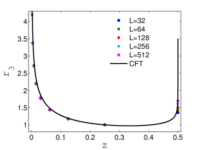
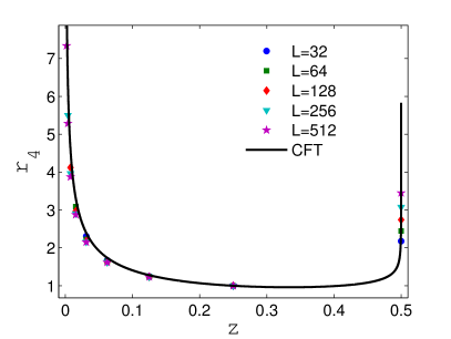
Figure 9: Entanglement for two adjacent intervals of equal length $\ell\leq L/2$ in a periodic chain of length $L$. The quantity $r_{n}(z)$ in Eq. (72) as function of $z=\ell/L$ compared with the parameter free CFT prediction for $n=3$ (left) and $n=4$ (right).

Following Ref. [25], we can construct quantities in which the dependence on the non-universal parameters $d_{n}$ and also the universal dependence on $L$ cancel. To this aim, it is enough to divide ${\rm Tr}(\rho_{A}^{T_{2}})^{n}$ by the value it assumes at a given fixed $\ell$, e.g. $\ell=L/4$, i.e. by considering the quantities

$$r_{n}(z)=\ln\frac{{\rm Tr}(\rho_{A}^{T_{A_{2}=\ell}})^{n}}{{\rm Tr}(\rho_{A}^{T_{A_{2}=L/4}})^{n}},$$ (72)

whose parameter free CFT predictions for $n$ even and odd are

$$r_{n_{e}}=\frac{1}{12}\Big{(}\frac{2}{n_{e}}-\frac{n_{e}}{2}\Big{)}\ln(2\sin^{2}(\pi z))-\frac{1}{12}\Big{(}\frac{n_{e}}{2}+\frac{1}{n_{e}}\Big{)}\ln(\sin(2\pi z)),$$

$$r_{n_{o}}=\frac{1}{24}\Big{(}\frac{1}{n_{o}}-n_{o}\Big{)}\ln(2\sin^{2}(\pi z)\sin(2\pi z)).$$ (73)

The numerical results for these quantities are shown in Fig. 9 for $n=3$ and $n=4$. The agreement between the numerical data and the CFT predictions is perfect for all considered values of $L$, showing that finite size corrections are very small for these quantities. Notice that for $z=1/2$ we have a bipartite system (i.e. $B\to\emptyset$) and the equations in (73) obviously do not work since the data are described by Eqs. (26) and (27), reflecting the fact that the limit $z\to 1/2$ is approached in a non-uniform way (i.e. the limits $z\to 1/2$ and $N\to\infty$ do not commute as obvious).

For the logarithmic negativity, we can analogously define the subtracted quantity

$$\epsilon(z)={\cal E}(\ell,L)-{\cal E}(L/4,L)=\frac{1}{8}\ln[\tan(\pi z)]\,,$$ (74)

and again the r.h.s. is a parameter free CFT prediction. In Fig. 10, this prediction is compared with the numerical data and the agreement is extremely good except at $z=1/2$ where the numerical data are described by the bipartite formula (28). Notice that finite size scaling corrections are even smaller than those for the quantities $r_{n}(z)$ in Fig. 9.

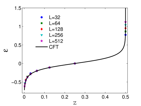
Figure 10: Entanglement negativity for two adjacent intervals of equal length $\ell<L/2$ in a periodic chain of length $L$: Subtracted negativity $\epsilon(z)$ in Eq. (74) compared with the parameter free CFT prediction.

5.2 Two disjoint intervals

In this section we study the most interesting and difficult situation of two disjoint intervals for which an accurate numerical study of the negativity has been already performed by means of density matrix renormalization group in Ref. [15], but before the systematic CFT derivation in Refs. [24, 25]. Here we first consider the traces ${\rm Tr}(\rho_{A}^{T_{2}})^{n}$ and ${\rm Tr}(\rho_{A})^{n}$. Indeed, although standard Rényi entropies given by ${\rm Tr}\rho_{A}^{n}$ have been already studied in Refs. [30, 38, 39], they show large corrections to the scaling which is worth recalling before embarking in the analysis of ${\rm Tr}(\rho_{A}^{T_{2}})^{n}$.

In order to determine numerically the function ${\cal F}_{n}(x)$, we calculate for several finite chains the quantity

$$F^{\rm lat}_{n}(x)=\frac{{\rm Tr}\rho_{A_{1}\cup A_{2}}^{n}}{{\rm Tr}\rho_{A_{1}}^{n}{\rm Tr}\rho_{A_{2}}^{n}}(1-x)^{(n-1/n)/12}\,,$$ (75)

which in the scaling limit should converge to the CFT prediction ${\cal F}_{n}(x)$. In a finite system of length $L$, the four-point ratio $x$ must be rewritten by replacing all distances by the corresponding chordal lengths. For two intervals of the same length $\ell$ at distance $r$ this reads

$$x=\left(\frac{\sin(\pi\ell/L)}{\sin(\pi(\ell+r)/L)}\right)^{2}\,.$$ (76)

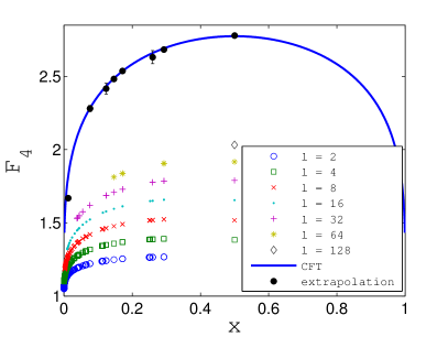
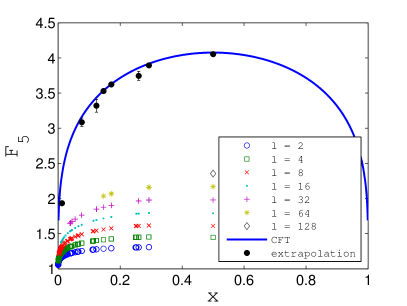
Figure 11: Numerical results for $F_{n}^{\rm lat}(x)$ as function of $x$ for different values of $\ell$ for $n=3$ (top left), $n=4$ (top right), and $n=5$ (bottom). The data are extrapolated to $\ell\to\infty$ by means of Eq. (78). The extrapolated data (topmost set of data) are in excellent agreement with the CFT prediction (continuous line).

The numerical data for the function $F^{\rm lat}_{n}(x)$ are reported in Fig. 11 for $n=3,4,5$ as function of $x$ for various values of $\ell$ (i.e. different values of $L$ according to Eq. (76)). It is evident that strong scaling corrections affect the data, as known from previous analyses [38, 39]. It has been argued on the basis of the general CFT arguments [72], and shown explicitly in few examples [71, 73, 74] both analytically and numerically, that the entanglement entropies (hence also the function $F^{\rm lat}_{n}(x)$), display ‘unusual’ corrections to the scaling which, at the leading order, can be effectively taken into account by the scaling ansatz

$$F_{n}^{\rm lat}(x)={\cal F}_{n}(x)+\ell^{-1/n}f_{n}(x)+\dots\,.$$ (77)

However, the corrections to the scaling in Fig. 11 cannot be captured by this simple ansatz because subleading corrections to the scaling become more and more important with increasing the value of $n$. Indeed, corrections of the form $\ell^{-m/n}$ for any integer $m$ are know to be present [73, 39, 40]. Thus the most general finite-$\ell$ ansatz is

$$F_{n}^{\rm lat}(x)={\cal F}_{n}(x)+\frac{f_{n}^{(1)}(x)}{\ell^{1/n}}+\frac{f_{n}^{(2)}(x)}{\ell^{2/n}}+\frac{f_{n}^{(3)}(x)}{\ell^{3/n}}\dots\,.$$ (78)

The effect of the subleading corrections is enhanced by the fact the amplitude functions $f_{n}^{(i)}(x)$ have different signs determining a non-monotonic behavior in $\ell$ (in particular, we have that $f^{(1)}_{n}$ is always negative, while $f^{(2)}_{n}$ and $f^{(3)}_{n}$ are always positive, as discussed in Ref. [40]). In order to have an accurate extrapolation to $\ell\to\infty$, for any $n$ we consider all the corrections above up to order $O(\ell^{-3/n})$ and we get the extrapolations reported in Fig. 11. The error bars are estimated by studying the stability of the extrapolation with respect to the number of sizes $\ell$ included in the fit. The overall agreement of the extrapolated points with the CFT prediction is excellent for all values of $x$ and for the three considered values of $n$, reproducing the results in Refs. [38, 39].

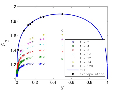
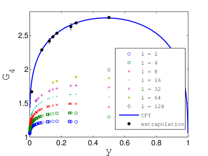
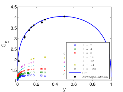
Figure 12: Numerical results for $G_{n}^{\rm lat}(x)$ as function of $y$ for different values of $\ell$ for $n=3$ (top left), $n=4$ (top right), and $n=5$ (bottom). The data are extrapolated to $\ell\to\infty$ by means of Eq. (80). The extrapolated data (topmost set of data) are in excellent agreement with the CFT prediction (continuous line).

After having summarized the corrections to the scaling for the entanglement entropies we can turn to the integer powers of the partial transpose in which we are interested here. In analogy with Eq. (75) we can define the lattice ratio

$$G^{\rm lat}_{n}(y)=\frac{{\rm Tr}(\rho_{A_{1}\cup A_{2}}^{T_{2}})^{n}}{{\rm Tr}\rho_{A_{1}}^{n}{\rm Tr}\rho_{A_{2}}^{n}}(1-y)^{(n-1/n)/12}\,,$$ (79)

that in the limit $\ell\to\infty$ is expected to converge to the CFT scaling function ${\cal G}_{n}(y)$ given by Eq. (53). In the case at hand, the numerical value of $y$ is given by the same expression in Eq. (76) for $x$. The numerical data for $G^{\rm lat}_{n}(y)$ are reported in Fig. 12 for $n=3,4,5$ as function of $y$ for various values of $\ell$. Also in this case, large scaling corrections are present. These are expected to be of the same form as for $F_{n}^{\rm lat}(x)$, i.e. described by the ansatz

$$G_{n}^{\rm lat}(y)={\cal G}_{n}(y)+\frac{g_{n}^{(1)}(y)}{\ell^{1/n}}+\frac{g_{n}^{(2)}(y)}{\ell^{2/n}}+\frac{g_{n}^{(3)}(y)}{\ell^{3/n}}\dots\,.$$ (80)

We repeat exactly the same analysis as for $F_{n}^{\rm lat}(x)$ to extrapolate the data to $\ell\to\infty$. As above, we find that $g^{(1)}_{n}$ is always negative, while $g^{(2)}_{n}$ and $g^{(3)}_{n}$ are positive. Using this observation, we extrapolate to $\ell\to\infty$, obtaining the results (with error bars) reported in Fig. 12. These points agree very well with the CFT prediction in Eq. (53) for the three values of $n$ considered.

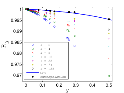
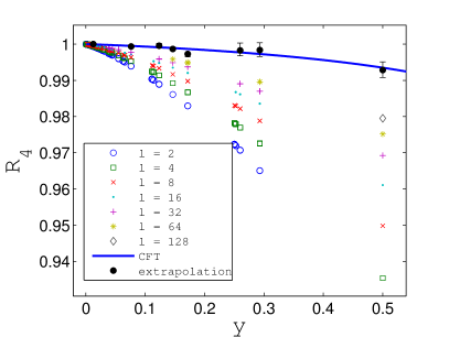
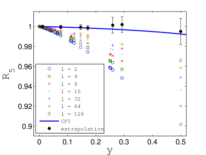
Figure 13: Numerical results for $R_{n}^{\rm lat}(x)$ as function of $y$ for different values of $\ell$ for $n=3$ (top left), $n=4$ (top right), and $n=5$ (bottom). The data are extrapolated to $\ell\to\infty$ by means of Eq. (82). The extrapolated data (topmost set of data) are in excellent agreement with the CFT prediction (continuous line).

It is evident from the comparison of Figs. 11 and 12 that the functions $G^{\rm lat}_{n}(y)$ and $F^{\rm lat}_{n}(y)$ are very close to each other and the logarithmic negativity is instead only determined by the small differences between the two. Thus, as already discussed in Sec. 3, a practical way to have more accurate tests of the CFT predictions which are sensitive to the small differences between the two universal functions ${\cal G}_{n}(y)$ and ${\cal F}_{n}(y)$ is to consider the ratio $R_{n}(y)$ between the two and the analogous lattice quantity

$$R_{n}^{\rm lat}(y)\equiv\frac{G_{n}^{\rm lat}(y)}{F_{n}^{\rm lat}(y)},$$ (81)

which in the limit $\ell\to\infty$ converges to the CFT prediction in Eq. (54). The numerical data for $R^{\rm lat}_{n}(y)$ are reported in Fig. 13 for $n=3,4,5$ as function of $y$ for different values of $\ell$. Once again, large scaling corrections are present and there are no accidental cancellations in the ratio, so that they are again expected to be of the same form as for $F_{n}^{\rm lat}(x)$, i.e. described by the ansatz

$$R_{n}^{\rm lat}(y)=R_{n}(y)+\frac{r_{n}^{(1)}(y)}{\ell^{1/n}}+\frac{r_{n}^{(2)}(y)}{\ell^{2/n}}+\frac{r_{n}^{(3)}(y)}{\ell^{3/n}}\dots\,.$$ (82)

We repeat again the same analysis as for $F_{n}^{\rm lat}(x)$ to extrapolate the data to $\ell\to\infty$ and the results (with error bars) are reported in Fig. 13. Unlike $f^{(j)}_{n}(x)$’s and $g^{(j)}_{n}(y)$’s, in this case the signs of $r^{(j)}_{n}(y)$’s are not defined (indeed $r^{(j)}_{n}$’s can be written as complicated combinations of $f^{(j)}_{n}$’s and $g^{(j)}_{n}$’s). For this reason, the error bars in Fig. 13 are larger than the ones in Fig. 11 and in Fig. 12. It is evident that the extrapolated points in Fig. 13 agree very well with the CFT prediction for the three considered values of $n$. It is very remarkable that the numerical calculations are accurate enough to detect the small differences of these ratios from $1$ (at least for $n=3$ and $n=4$, while for $n=5$ the estimated error is too large to distinguish the extrapolation from one).

Figure 14: Logarithmic negativity for two intervals of equal length $\ell$ at distance $r$ as function of the four point ratio $y$.

Finally we turn to the study of the logarithmic negativity ${\cal E}$. The numerical data as a function of $y$ are reported in Fig. 14 for several values of $\ell$. In the figure all data collapse on a single curve, with some tiny corrections to the scaling for the smaller values of $\ell$, which however are much smaller than the scaling corrections for the ratios $R_{n}(y)$, as evident from a comparison between Fig. 14 and Fig. 13. This is similar to what has been observed for the free boson in Ref. [25] and recalls the similar effect for the entanglement entropies both for one and two intervals where the unusual corrections to the scaling are suppressed for the von Neumann entropy for periodic boundary conditions [71, 73]. It would be then interesting to study the negativity for Ising chains with open boundary conditions to check whether the unusual corrections are enhanced (analogously to Friedel oscillations [75, 76]). On the more theoretical side, we have not been able to find the analytic continuation of $R_{n_{e}}(y)$ to $n_{e}\to 1$ which would allow a strict check of the numerical data in Fig. 14. However, the data for $y\ll 1$ are very close to zero in agreement with the general result [25] that the negativity should fall off faster than any power with the separation of the intervals.

6 Conclusions

In this manuscript we presented a systematic study of the entanglement negativity and of the traces of integer powers of the partial transpose of the reduced density matrix in the critical Ising chain. In order to have an accurate numerical evaluation of these quantities we adapted the tree tensor network technique to the calculation of the eigenvalues of the partially transposed reduced density matrix. For two adjacent intervals we found perfect agreement with the model independent CFT predictions in Refs. [24, 25]. For two disjoint intervals we first derived a CFT prediction for ${\rm Tr}(\rho_{A_{1}\cup A_{2}}^{T_{2}})^{n}$ which later has been compared with the numerical data taking into account the finite size corrections induced by the finite length of the blocks. Unfortunately, in order to determine the logarithmic negativity, it remains a hard open problem to find the analytic continuation to $n_{e}\to 1$ of these traces. This reflects the similar problem found for the standard entanglement entropies, where explicit formulas for ${\rm Tr}\rho_{A_{1}\cup A_{2}}^{n}$ have been obtained for some models [29, 30], but they have not been analytically continued to $n\to 1$, preventing us to write down a close formula for the von Neumann entropy.

References

References

- [1] L. Amico, R. Fazio, A. Osterloh, and V. Vedral, Entanglement in many-body systems, Rev. Mod. Phys. 80, 517 (2008); J. Eisert, M. Cramer, and M. B. Plenio, Area laws for the entanglement entropy - a review, Rev. Mod. Phys. 82, 277 (2010); Entanglement entropy in extended systems, P. Calabrese, J. Cardy, and B. Doyon Eds, J. Phys. A 42 500301 (2009).
- [2] P. Calabrese and A. Lefevre, Entanglement spectrum in one-dimensional systems, Phys. Rev. A 78, 032329 (2008).
- [3] C. Holzhey, F. Larsen, and F. Wilczek, Geometric and renormalized entropy in conformal field theory, Nucl. Phys. B 424, 443 (1994).
- [4] P. Calabrese and J. Cardy, Entanglement entropy and quantum field theory, J. Stat. Mech. P06002 (2004).
- [5] G. Vidal, J. I. Latorre, E. Rico, and A. Kitaev, Entanglement in quantum critical phenomena, Phys. Rev. Lett. 90, 227902 (2003); J. I. Latorre, E. Rico, and G. Vidal, Ground state entanglement in quantum spin chains, Quant. Inf. Comp. 4, 048 (2004).
- [6] P. Calabrese and J. Cardy, Entanglement entropy and conformal field theory, J. Phys. A 42, 504005 (2009).
- [7] J. Cardy, The ubiquitous ’c’: from the Stefan-Boltzmann law to quantum information, J. Stat. Mech. (2010) P10004.
- [8] M. Fagotti, P. Calabrese, and J. E. Moore, Entanglement spectrum of random-singlet quantum critical points, Phys. Rev. B 83, 045110 (2011).
- [9] M. B. Plenio and S. Virmani, An introduction to entanglement measures, Quant. Inf. Comput. 7, 1 (2007).
- [10] G. Vidal, Entanglement monotones, J. Mod. Opt. 47 (2000) 355.
- [11] J. Eisert and M. B. Plenio, A Comparison of entanglement measures, J. Mod. Opt. 46, 145 (1999).
- [12] A. Peres, Separability criterion for density matrices, Phys. Rev. Lett. 77, 1413 (1996); M. Horodecki, P. Horodecki and R. Horodecki, Mixed state entanglement and distillation: Is there a ‘bound’ entanglement in nature?, Phys. Rev. Lett. 80, 5239 (1998); K. Zyczkowski, P. Horodecki, A. Sanpera and M. Lewenstein, On the volume of the set of mixed entangled states, Phys. Rev. A 58, 883 (1998); L. M. Duan, G. Giedke, J. I. Cirac and P. Zoeller, Inseparability criterion for continuos variables systems, Phys. Rev. Lett. 84, 2722 (2000); R. Simon, Peres-Horodecki separability criterion for continuos variables systems, Phys. Rev. Lett. 84, 2726 (2000).
- [13] G. Vidal and R. F. Werner, A computable measure of entanglement, Phys. Rev. A 65, 032314 (2002).
- [14] K. Audenaert, J. Eisert, M. B. Plenio, and R. F. Werner, Entanglement Properties of the Harmonic Chain, Phys. Rev. A 66, 042327 (2002).
- [15] H. Wichterich, J. Molina-Vilaplana, and S. Bose, Scale invariant entanglement at quantum phase transitions, Phys. Rev. A 80, 010304 (2009).
- [16] S. Marcovitch, A. Retzker, M. B. Plenio, and B. Reznik, Critical and noncritical long range entanglement in the Klein-Gordon field, Phys. Rev. A 80, 012325 (2009).
- [17] H. Wichterich, J. Vidal, and S. Bose, Universality of the negativity in the Lipkin-Meshkov-Glick model, Phys. Rev. A 81, 032311 (2010).
- [18] A. Bayat, P. Sodano, and S. Bose, Negativity as the Entanglement Measure to Probe the Kondo Regime in the Spin-Chain Kondo Model, Phys. Rev. B 81, 064429 (2010).
- [19] R. Santos, V. Korepin, and S. Bose, Negativity for two blocks in the one dimensional Spin 1 AKLT model, Phys. Rev. A 84, 062307 (2011).
- [20] R. Santos and V. Korepin, Entanglement of disjoint blocks in the one dimensional Spin 1 VBS, J. Phys. A 45, 125307 (2012)
- [21] A. Bayat, S. Bose, P. Sodano, and H. Johannesson, Entanglement probe of two-impurity Kondo physics in a spin chain, Phys. Rev. Lett. 109, 066403 (2012).
- [22] A. Bayat, P. Sodano, and S. Bose, Entanglement Routers Using Macroscopic Singlets, Phys. Rev. Lett. 105, 187204 (2010).
- [23] P. Sodano, A. Bayat, and S. Bose, Kondo Cloud Mediated Long Range Entanglement After Local Quench in a Spin Chain, Phys. Rev. B 81, 100412 (2010).
- [24] P. Calabrese, J. Cardy, and E. Tonni, Entanglement negativity and quantum field theory, Phys. Rev. Lett. 109, 130502 (2012).
- [25] P. Calabrese, J. Cardy, and E. Tonni, Entanglement negativity in extended systems: a quantum field theory approach, J. Stat. Mech. (2013) P02008.
- [26] J. L. Cardy, O.A. Castro-Alvaredo, and B. Doyon, Form factors of branch-point twist fields in quantum integrable models and entanglement entropy, J. Stats. Phys. 130 (2008) 129.
- [27] P. Di Francesco, P. Mathieu, and D. Senechal, Conformal Field Theory (Springer-Verlag, New York, 1997).
- [28] S. Furukawa, V. Pasquier, and J. Shiraishi, Mutual information and compactification radius in a c=1 critical phase in one dimension, Phys. Rev. Lett. 102, 170602 (2009).
- [29] P. Calabrese, J. Cardy, and E. Tonni, Entanglement entropy of two disjoint intervals in conformal field theory, J. Stat. Mech. P11001 (2009).
- [30] P. Calabrese, J. Cardy, and E. Tonni, Entanglement entropy of two disjoint intervals in conformal field theory II, J. Stat. Mech. P01021 (2011).
- [31] H. Casini, C. D. Fosco, and M. Huerta, Entanglement and alpha entropies for a massive Dirac field in two dimensions, J. Stat. Mech. P05007 (2005); H. Casini and M. Huerta, Remarks on the entanglement entropy for disconnected regions, JHEP 0903: 048 (2009); H. Casini and M. Huerta, Reduced density matrix and internal dynamics for multicomponent regions, Class. Quant. Grav. 26, 185005 (2009); H. Casini, Entropy inequalities from reflection positivity, J. Stat. Mech. (2010) P08019; D. D. Blanco and H. Casini, Entanglement entropy for non-coplanar regions in quantum field theory Class. Quant. Grav. 28, 215015 (2011).
- [32] P. Calabrese, Entanglement entropy in conformal field theory: New results for disconnected regions, J. Stat. Mech. (2010) P09013.
- [33] M. Headrick, Entanglement Renyi entropies in holographic theories, Phys. Rev. D 82, 126010 (2010).
- [34] M. A. Rajabpour and F. Gliozzi, Entanglement entropy of two disjoint intervals from fusion algebra of twist fields, J. Stat. Mech. (2012) P02016.
- [35] S. Ryu and T. Takayanagi, Holographic derivation of entanglement entropy from AdS/CFT, Phys. Rev. Lett. 96 (2006) 181602; S. Ryu and T. Takayanagi, Aspects of holographic entanglement entropy, JHEP 0608: 045 (2006); V. E. Hubeny and M. Rangamani, Holographic entanglement entropy for disconnected regions, JHEP 0803: 006 (2008); M Headrick and T Takayanagi, A holographic proof of the strong subadditivity of entanglement entropy, Phys. Rev. D 76, 106013 (2007); T. Nishioka, S. Ryu, and T. Takayanagi, Holographic entanglement entropy: an overview, J. Phys. A 42 (2009) 504008; E. Tonni, Holographic entanglement entropy: near horizon geometry and disconnected regions, JHEP 1105:004 (2011); J. Molina-Vilaplana and P. Sodano, Holographic View on Quantum Correlations and Mutual Information between Disjoint Blocks of a Quantum Critical System, JHEP 10 (2011) 011; M. Headrick, A. Lawrence, and M. M. Roberts, Bose-Fermi duality and entanglement entropies, arXiv:1209.2428; I. A. Morrison and M. M. Roberts, Mutual information between thermo-field doubles and disconnected holographic boundaries, arXiv:1211.2887.
- [36] P. Facchi, G. Florio, C. Invernizzi, and S. Pascazio, Entanglement of two blocks of spins in the critical Ising model, Phys. Rev. A 78, 052302 (2008).
- [37] F. Igloi and I. Peschel, On reduced density matrices for disjoint subsystems, 2010 EPL 89 40001.
- [38] V. Alba, L. Tagliacozzo, and P. Calabrese, Entanglement entropy of two disjoint blocks in critical Ising models, Phys. Rev. B 81 060411 (2010).
- [39] M. Fagotti and P. Calabrese, Entanglement entropy of two disjoint blocks in XY chains, J. Stat. Mech. (2010) P04016.
- [40] V. Alba, L. Tagliacozzo, and P. Calabrese, Entanglement entropy of two disjoint intervals in theories, J. Stat. Mech. (2011) P06012.
- [41] H. F. Song, S. Rachel, C. Flindt, I. Klich, N. Laflorencie, and K. Le Hur, Bipartite fluctuations as a probe of many-body entanglement, Phys. Rev. B 85, 035409 (2012); B. Swingle, Rényi entropy, mutual information, and fluctuation properties of Fermi liquids, Phys. Rev. B 86, 045109 (2012); P. Calabrese, M. Mintchev, and E. Vicari, Exact relations between particle fluctuations and entanglement in Fermi gases, EPL 98, 20003 (2012).
- [42] M. Fagotti, New insights into the entanglement of disjoint blocks, EPL 97, 17007 (2012).
- [43] L. J. Dixon, D. Friedan, E. J. Martinec and S. H. Shenker, The Conformal Field Theory of Orbifolds, Nucl. Phys. B 282 (1987) 13.
- [44] Al. B. Zamolodchicov, Conformal scalar field on the hyperelliptic curve and critical Ashkin-Teller multipoint correlation functions, Nucl. Phys. B 285 (1987) 481.
- [45] R. Dijkgraaf, E. P. Verlinde and H. L. Verlinde, C = 1 Conformal Field Theories on Riemann Surfaces, Commun. Math. Phys. 115 (1988) 649.
- [46] L. Alvarez-Gaume, G. W. Moore and C. Vafa, Theta Functions, Modular Invariance and Strings, Commun. Math. Phys. 106 (1986) 1.
- [47] V. G. Knizhnik, Analytic Fields on Riemann Surfaces II, Commun. Math. Phys. 112, (1987) 567.
- [48] L. Alvarez-Gaume, J. B. Bost, G. W. Moore, P. C. Nelson and C. Vafa, Bosonization on Higher Genus Riemann Surfaces, Commun. Math. Phys. 112 (1987) 503.
- [49] D. Bernard, Twisted Fields And Bosonization On Riemann Surfaces, Nucl. Phys. B 302 (1988) 251.
- [50] V. Alba, Entanglement negativity and conformal field theory: a Monte Carlo study, to appear.
- [51] J. L. Cardy, Operator Content of Two-Dimensional Conformally Invariant Theories, Nucl. Phys. B 270, 186 (1986).
- [52] A. Erderlyi, Higher transcendental functions, vol. I, Mc Graw Hill, (1953).
- [53] S. Sachdev, Quantum Phase Transitions, Cambridge University Press, 2001.
- [54] M. Caraglio and F. Gliozzi, Entanglement entropy and twist fields, JHEP 0811: 076 (2008).
- [55] F. Gliozzi and L. Tagliacozzo, Entanglement entropy and the complex plane of replicas, J. Stat. Mech. P01002 (2010).
- [56] J. I. Cirac and F. Verstraete, Renormalization and tensor product states in spin chains and lattices, J. Phys. A 42, 504004 (2009); G. Vidal, Entanglement Renormalization: an introduction, in Understanding Quantum Phase Transitions, ed. by L. D. Carr (Taylor & Francis, Boca Raton, 2010) arXiv:0912.1651.
- [57] Y. Shi, L. Duan, and G. Vidal, Classical simulation of quantum many-body systems with a tensor network, Phys. Rev. A 74, 022320 (2006).
- [58] L. Tagliacozzo, G. Evenbly, and G. Vidal, Simulation of two-dimensional quantum system using a tree tensor network that exploits the area law, Phys. Rev. B 80, 235127 (2009).
- [59] M. Fannes, B. Nachtergaele, and R. Werner, Ground states of VBS models on Cayley trees, J. Stat. Phys. 66, 939 (1992).
- [60] B. Friedman, A density matrix renormalization group approach to interacting quantum systems on Cayley trees, J. Phys.: Cond. Mat. 42, 9, 9021 (1997).
- [61] M. Lepetit, M. Cousy, and G. Pastor, Density-matrix renormalization study of the Hubbard model on a Bethe lattice, European Physical Journal B 13, 421 (2000).
- [62] M. Martin-Delgado, J. Rodriguez-Laguna, and G. Sierra, Density-Matrix renormalization-group study of excitons in dendrimers, Phys. Rev. B 65, 155116 (2002).
- [63] D. Nagaj, E. Farhi, J. Goldstone, P. Shor, and I. Sylverster, The Quantum Transverse Field Ising Model on an Infinite Tree from Matrix Product States, Phys. Rev. B 77, 214431 (2008).
- [64] P. Silvi, V. Giovannetti, S. Montangero, M. Rizzi, J. Cirac ,and R. Fazio, Critical properties of homogeneous binary trees, Phys. Rev. A 81, 062335 (2010).
- [65] R. Hübener, V. Nebendahl, and W. Dür, Concatenated tensor network states, New J. Phys. 12, 025004 (2010).
- [66] V. Murg, F. Verstraete, Ö. Legeza, and R. Noack, Simulating Strongly Correlated Quantum Systems with Tree Tensor Networks, Phys. Rev. B 82, 205105 (2010).
- [67] R. Hübener, C. Kruszynska, L. Hartmann, W. Dür, M. Plenio, and J. Eisert, Tensor network methods with graph enhancement, Phys. Rev. B 84, 125103 (2011).
- [68] L. Tagliacozzo and G. Vidal, Entanglement renormalization and gauge symmetry, Phys. Rev. B 83, 115127 (2011).
- [69] G. Evenbly and G. Vidal, Quantum Criticality with the Multi-scale Entanglement Renormalization Ansatz., arXiv:1109.5334.
- [70] A. Ferris and G. Vidal, Perfect Sampling with Unitary Tensor Networks, Phys. Rev. B 85, 165146 (2012).
- [71] P. Calabrese, M. Campostrini, F. Essler, and B. Nienhuis, Parity effects in the scaling of block entanglement in gapless spin chains, Phys. Rev. Lett. 104, 095701 (2010).
- [72] J. Cardy and P. Calabrese, Unusual corrections to scaling in entanglement entropy, J. Stat. Mech. (2010) P04023.
- [73] P. Calabrese and F. H. L. Essler, Universal corrections to scaling for block entanglement in spin-1/2 XX chains, J. Stat. Mech. (2010) P08029.
- [74] J. C. Xavier and F. C. Alcaraz, Renyi entropy and parity oscillations of anisotropic spin-s Heisenberg chains in a magnetic field, Phys. Rev. B 83, 214425 (2011); M. Dalmonte, E. Ercolessi, L. Taddia, Estimating quasi-long-range order via Renyi entropies, Phys. Rev. B 84, 085110 (2011); M. Dalmonte, E. Ercolessi, L. Taddia, Critical properties and Renyi entropies of the spin-3/2 XXZ chain, Phys. Rev. B 85, 165112 (2012); P. Calabrese, M. Mintchev, and E. Vicari, The entanglement entropy of one-dimensional systems in continuous and homogeneous space, J. Stat. Mech. P09028 (2011).
- [75] N. Laflorencie, E. S. Sorensen, M.-S. Chang, and I. Affleck, Boundary effects in the critical scaling of entanglement entropy in 1D systems, Phys. Rev. Lett. 96, 100603 (2006).
- [76] M. Fagotti and P. Calabrese, Universal parity effects in the entanglement entropy of XX chains with open boundary conditions, J. Stat. Mech. P01017 (2011).