Entanglement negativity and conformal field theory: a Monte Carlo study

Abstract

We investigate the behavior of the moments of the partially transposed reduced density matrix $\rho^{T_{2}}_{A}$ in critical quantum spin chains. Given subsystem $A$ as union of two blocks, this is the (matrix) transposed of $\rho_{A}$ with respect to the degrees of freedom of one of the two. This is also the main ingredient for constructing the logarithmic negativity. We provide a new numerical scheme for calculating efficiently all the moments of $\rho_{A}^{T_{2}}$ using classical Monte Carlo simulations. In particular we study several combinations of the moments which are scale invariant at a critical point. Their behavior is fully characterized in both the critical Ising and the anisotropic Heisenberg XXZ chains. For two adjacent blocks we find, in both models, full agreement with recent CFT calculations. For disjoint ones, in the Ising chain finite size corrections are non negligible. We demonstrate that their exponent is the same governing the unusual scaling corrections of the mutual information between the two blocks. Monte Carlo data fully match the theoretical CFT prediction only in the asymptotic limit of infinite intervals. Oppositely, in the Heisenberg chain scaling corrections are smaller and, already at finite (moderately large) block sizes, Monte Carlo data are in excellent agreement with the asymptotic CFT result.

1 Introduction

In recent years there has been a growing interest in characterizing the behavior of entanglement related quantities (see [1] for general reviews) in many body quantum systems. Moreover, the deep connection between entanglement and conformal field theory (CFT) [1, 2, 3, 4] has boosted a huge amount of work at the frontiers between quantum information, condensed matter, and quantum field theory.

Entanglement related quantities are usually constructed considering a bipartition of a system $S$ into two subsystems as $S=A\cup B$. Given the (pure) state $|\psi\rangle$ of the total system and the density matrix $\rho\equiv|\psi\rangle\langle\psi|$, the reduced density matrix for subsystem $A$ is obtained by tracing over the degrees of freedom of $B$ as $\rho_{A}\equiv\Tr_{B}\rho$. The entanglement between $A$ and $B$ can be quantified using the von Neumann entropy $S_{A}\equiv-\Tr\rho_{A}\log\rho_{A}$. Alternatively, from the $n-$th moment $\Tr(\rho_{A}^{n})(n\in{\mathbb{N}}$) of the reduced density matrix one can construct the so called Rényi entropies $S_{A}^{(n)}\equiv 1/(n-1)\log\Tr(\rho_{A})^{n}$, which are also standard entanglement measures. The von Neumann entropy is recovered from the Rényi entropies as the analytic continuation $S_{A}=\lim_{n\to 1}S_{A}^{(n)}$.

Let us now consider a 1D critical quantum system (spin chain) described in the scaling limit by a conformal field theory (CFT). After restricting to periodic boundary conditions, and taking subsystem $A$ a single interval (Fig. 1 ($\bf a$)), the scaling behavior of the Rényi entropies is given as [2, 3, 4, 5, 6]

$$S_{A}^{(n)}=\frac{c}{6}\left(1+\frac{1}{n}\right)\log\frac{\ell}{a}+c^{\prime}_{n}$$ (1)

with $\ell$ the length of the interval. Here $c$ is the celebrated central charge [7], $a$ an ultraviolet cutoff (lattice spacing), and $c^{\prime}_{n}$ a non universal constant. From (1) the von Neumann entropy $S_{A}$ is obtained as

$$S_{A}=\frac{c}{3}\log\frac{\ell}{a}+\tilde{c}_{1}$$ (2)

with $\tilde{c}_{1}$ also non universal.

Both (1)(2) are nowadays accepted as the standard tools to extract the central charge in 1D critical systems, while other universal features can be obtained by analyzing their finite size corrections [8, 9, 10, 11, 12, 13].

From the field theory point of view, much more information about the underlying CFT is contained in the mutual information between two intervals [14, 15, 16, 17, 18, 19, 20, 21, 22, 23, 24, 25, 26, 27, 28]. In fact, given $A$ as sum of two non complementary blocks as $A\equiv A_{1}\cup A_{2}$ (Fig. 1 (c)), their mutual information $I^{(n)}_{A_{1}:A_{2}}\equiv S^{(n)}_{A_{1}}+S^{(n)}_{A_{2}}-S^{(n)}_{A_{1}\cup A_{2}}$ gives access to the full operator content of a CFT [29]. From the quantum information perspective, however, since subsystem $A$ is not in general in a pure state, $I^{(n)}_{A_{1}:A_{2}}$ is not a measure of the mutual entanglement between $A_{1},A_{2}$, although it contains information about the correlations between them. A standard measure of the entanglement between two blocks is instead the so-called logarithmic negativity [30]. Denoting a basis for the Hilbert space of $A_{1}$($A_{2}$) as $|e_{i}^{(1)}\rangle$ ($|e_{j}^{(2)}\rangle$), one first defines the partially transposed reduced density matrix (with respect to $A_{2}$) $\rho^{T_{2}}_{A}$ as

$$\langle e_{i}^{(1)}\otimes e_{j}^{(2)}|\rho_{A}^{T_{2}}|e_{k}^{(1)}\otimes e_{l}^{(2)}\rangle\equiv\langle e_{i}^{(1)}\otimes e_{l}^{(2)}|\rho_{A}|e_{k}^{(1)}\otimes e_{j}^{(2)}\rangle$$ (3)

Then the logarithmic negativity is readily given by

$${\cal E}\equiv\log||\rho_{A}^{T_{2}}||_{1}$$ (4)

with $||\rho_{A}^{T_{2}}||_{1}$ denoting the trace norm, i.e. the sum of the absolute values of the eigenvalues of $\rho_{A}^{T_{2}}$. Besides its importance in quantum information, it has been pointed out recently that the logarithmic negativity is a universal quantity at a second order phase transition [31], which makes ${\cal E}$ a usable indicator of critical behavior in quantum many body systems.

Arguably in the context of field theories a major role is played by the moments of $\rho_{A}^{T_{2}}$, i.e. $\Tr(\rho_{A}^{T_{2}})^{n}$. In particular, the recent CFT approach developed in Ref. [32, 33] provided full analytical understanding of their scaling behavior, for both adjacent and disjoint intervals (Fig. 1 (b) and (c)). In the former case this allowed, via the analytic continuation $n\to 1$, to obtain an exact expression for ${\cal E}$. For two disjoint intervals, although it was not possible to perform the analytic continuation, it has been proven rigorously that at a second order phase transition $\cal E$ is a universal function of the (dimensionless) harmonic ratio

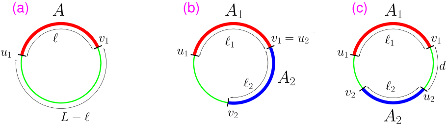
Figure 1: Different ways of partitioning a 1D spin chain (of length $L$) considered in this work. Subsystem $A$ is denoted with the thicker line. (a) $A$ is the single interval $A\equiv[u_{1},v_{1}]$ (of length $\ell=|v_{1}-u_{1}|$). (b) $A$ is made of two adjacent intervals $A=A_{1}\cup A_{2}\equiv[u_{1},v_{1}]\cup[u_{2},v_{2}]$ (of length respectively $\ell_{1}=|v_{1}-u_{1}|$ and $\ell_{2}=|v_{2}-u_{2}|$). (c) Two disjoint intervals $A_{1},A_{2}$ at distance $d=|u_{2}-v_{1}|$. In this work we always consider intervals of equal length, i.e. $\ell_{1}=\ell_{2}=\ell$.

$$y\equiv\frac{(v_{1}-u_{1})(v_{2}-u_{2})}{(u_{2}-u_{1})(v_{2}-v_{1})}$$ (5)

with $u_{i},v_{i}$ the endpoints of the two blocks (cf. Fig 1). Yet, we should mention that the analytical treatment of $\rho_{A}^{T_{2}}$ is a hard task (results are available only for free bosons [34] [32, 33]), and, as a matter of fact, a precise verification of the above mentioned CFT findings in microscopic models was up to now lacking.

In this work we demonstrate that all the moments of $\rho_{A}^{T_{2}}$ can be efficiently computed in classical Monte Carlo simulations exploiting the mapping between a quantum system in $d$ dimensions and a classical one in $d+1$. The Monte Carlo technique we propose, which is itself one of our main results, generalizes the one used in Ref. [15, 21, 22, 35] to compute $\Tr\rho_{A}^{n}$ (and the Rényi mutual information thereof), allowing us to provide a robust verification of the CFT results in Ref. [32, 33]. To this purpose, following [32, 33], it is convenient to define for adjacent blocks the ratio $r_{n}$  as

$$r_{n}(z)\equiv\frac{\Tr(\rho_{A_{1}\cup A_{2}}^{T_{2}=\ell})^{n}}{\Tr(\rho_{A_{1}\cup A_{2}}^{T_{2}=L/4})^{n}}$$ (6)

with $z\equiv\ell/L$. Here the notation $\Tr\rho_{A}^{T_{2}=\ell(L/4)}$ means that the partial transposition is done with respect to the degrees of freedom of block $A_{2}$ of length $\ell(L/4)$. For two disjoint blocks we use instead the ratio $R_{n}(y)$

$$R_{n}(y)\equiv\frac{\Tr(\rho_{A_{1}\cup A_{2}}^{T_{2}=\ell})^{n}}{\Tr\rho_{A_{1}\cup A_{2}}^{n}}$$ (7)

Remarkably both $r_{n}$ and $R_{n}$ are scale invariant quantities at a second order transition (cf. [32, 33] or section 2), which makes them good indicators for quantum and classical critical behaviors. In particular, a part from scaling corrections, which are expected to be less severe for ${\cal E}$ [32], they are as effective as the logarithmic negativity. Also, their being not related to any local order parameter makes them suitable especially for detecting topological transitions. On the CFT side, we anticipate here that (cf. section 2), while the scaling function $r_{n}(z)$ is fully characterized in terms of the central charge, $R_{n}(y)$ is a universal function of $y$ and depends on the full operator content of the given theory. In this sense $R_{n}(y)$ provides yet another tool (besides the mutual information) to unveil the deep structure of CFTs.

The models.

In this work we focus on the critical Ising quantum spin chain and the anisotropic Heisenberg XXZ model at $\Delta=-1/\sqrt{2}$ ($\Delta$ is the anisotropy). In both cases we consider periodic boundary conditions. The Ising chain in a transverse field $h$ is defined in terms of the Hamiltonian

$${\mathcal{H}}^{Is}=-\sum\limits_{i}[\sigma_{i}^{x}\sigma_{i+1}^{x}+h\sigma_{i}^{z}]$$ (8)

with $\sigma_{i}^{x,y,z}$ the Pauli matrices and $i=1,2,\dots,L$. The model exhibits a ferromagnetic (paramagnetic) phase for $h<1$ ($h>1$) with a second order phase transition at the critical value $h_{c}=1$. Its critical behavior is described in the continuum by the free Majorana fermion theory, which is the simplest and most studied CFT (with $c=1/2$). The same theory describes the critical behavior of the 2D classical Ising model.

The anisotropic Heisenberg XXZ spin chain is instead defined by the interaction

$${\mathcal{H}}^{XXZ}=\sum\limits_{i=1}^{L}(\sigma^{x}_{i}\sigma^{x}_{i+1}+\sigma^{y}_{i}\sigma^{y}_{i+1})~{}+~{}\Delta\sum\limits_{i=1}^{L}\sigma^{z}_{i}\sigma^{z}_{i+1}$$ (9)

Its phase diagram shows a critical liquid phase for $-1<\Delta\leq 1$ and a gapped one at $|\Delta|>1$ (the point $\Delta=-1$ is critical but not conformal invariant). The liquid phase is described in the continuum limit by the free compactified boson theory (or Luttinger liquid), which is a conformal field theory with $c=1$ [36, 37]. The region at $-1<\Delta\leq-1/\sqrt{2}$ is also mapped into the low-temperature critical phase of the 2D classical XY model, which describes a system of interacting classical spins (rotors) $\vec{S}_{i}\equiv(\cos\theta_{i},\sin\theta_{i})$ and is defined by the Hamiltonian

$${\mathcal{H}}^{2D\,XY}\equiv-\beta\sum\limits_{\langle ij\rangle}\textrm{Re}[\bar{\psi}_{i}\psi_{j}]=-\beta\sum\limits_{\langle ij\rangle}\vec{S}_{i}\cdot\vec{S}_{j}=-\beta\sum\limits_{\langle ij\rangle}\cos(\theta_{i}-\theta_{j})$$ (10)

Here $\psi_{i}\equiv e^{i\theta_{i}}\in U(1)$ are phases living on a two dimensional square lattice, $\beta=1/T$, and $\langle ij\rangle$ denotes nearest-neighbor sites. The XY model exhibits a low-temperature gapless critical phase characterized by quasi-long-range order (QLRO). This is divided from the standard paramagnetic phase at high temperature by a Berezinskii-Kosterlitz-Thouless (BKT) topological transition at $\beta_{BKT}=1.1199(1)$ [38, 39, 40, 41, 42, 43]. The critical properties at the BKT point are the same as in the XXZ chain at $\Delta=-1/\sqrt{2}$, a part from logarithmic corrections that are present only in the classical model.

Summary of the results.

The main results of this work can be summarized as follows. For two adjacent blocks, in both the critical Ising and XXZ chains and already for finite (large) $\ell$, the ratio $r_{n}(z)$ is numerically indistinguishable from its asymptotic value (i.e. at $L,\ell\to\infty$), meaning that scaling corrections are small. Moreover, Monte Carlo data are in full agreement (for any value of $z$) with the CFT result in Ref. [32].

For disjoint intervals we focus on $R_{3}(y)$. For the Ising chain unusual (in the sense of Ref. [10]) scaling corrections are non negligible, as observed for the mutual information [17, 21, 22, 23, 27] (see also [32, 33]). We numerically demonstrate that they decay as $\ell^{-\omega_{3}}$ with $\omega_{3}=1/3$, in agreement with the general behavior (as $\ell^{-1/n}$) found in the case of the mutual information. This allows to conclude that scaling corrections are the same for both quantities. By a standard finite size scaling analysis we then show that the asymptotic scaling function $R_{3}(y)$ perfectly matches the CFT. In the Heisenberg chain both usual and unusual scaling corrections are smaller, and already at $\ell\sim 50$ Monte Carlo data for $R_{3}(y)$ are in excellent agreement with the CFT result.

2 Negativity and Conformal Field Theory: general results

In the next sections we briefly review the scaling behavior of $r_{n}(z),R_{n}(y)$ in a generic system described by conformal field theory (cf. [32, 33] for more details). In order to make the manuscript self contained we start recalling some basic facts about $\Tr\rho_{A}^{n}$ and the mutual information (which enter in the construction of $R_{n}(y)$) in section 2.1. Then the behavior of $r_{n}$ and $R_{n}$ is discussed in section 2.2. Finally in 3 and 4 we specialize the result for $R_{n}(y)$ to the two cases of interest: the Ising universality class and the free compactified boson (Luttinger liquid). The result for the Luttinger liquid has been derived already in [33], whereas the one for the Ising is derived here  using the results of Ref. [32].

2.1 The moments of $\rho_{A}$ (Rényi entropies) & the mutual information

Let us consider a 1D system described by a conformal field theory and take as subsystem $A$ a single interval (as in Fig. 1 (a)) of length $\ell\equiv|v_{1}-u_{1}|$. The asymptotic scaling behavior of the moments $\Tr\rho_{A}^{n}$ of the reduced density matrix is given as

$$\Tr\rho_{A}^{n}=c_{n}\ell^{-\frac{c}{6}(n-\frac{1}{n})}$$ (11)

with $c_{n}$ a non universal constant and $c$ the central charge of the CFT. As shown by Calabrese and Cardy in Ref. [3], the $n$-th moment of the reduced density matrix can be also obtained in field theory in terms of a path integral $Z_{n}$ over the so-called $n$-sheeted Riemann surface ${\cal R}_{n}$ as

$$\Tr\rho_{A}^{n}=\frac{Z_{n}}{Z^{n}}$$ (12)

where $Z$ is the same path integral (but on the plane) and ensures the correct normalization $\Tr\rho_{A}=1$. It is worth observing that (12) lies at the heart of all the algorithms for calculating Rényi entropies in both classical and quantum Monte Carlo simulations [15, 21, 22, 45] (as it will be better clarified in section 5).

On the field theory side one further notices that (12) can be rewritten in terms of the so-called branch point twist fields ${\cal T}$ (and anti-twist $\bar{\cal T}$) as

$$\textrm{Tr}\rho_{A}^{n}=\langle{\cal T}_{n}(u_{1})\bar{\cal T}_{n}(v_{1})\rangle$$ (13)

The twist(and anti-twist) fields are primary fields (in the CFT language) and are inserted respectively at the endpoints $u_{1}$ and $v_{1}$ of interval $A$ (Fig. 1). Their scaling dimensions $\Delta_{n}=\bar{\Delta}_{n}$ are given as

$$\Delta_{n}=\frac{c}{12}\Big{(}n-\frac{1}{n}\Big{)}$$ (14)

Using (14) and basic properties of correlation functions, it is a simple exercise in CFT to obtain (11) from (13).

For two disjoint intervals (see Fig. 1 ($\bf c$)) the moments $\Tr\rho_{A_{1}\cup A_{2}}^{n}$ admit a similar representation in terms of twist fields and one now obtains the four point function

$$\Tr\rho_{A_{1}\cup A_{2}}^{n}=\langle{\cal T}_{n}(u_{1})\bar{\cal T}_{n}(v_{1}){\cal T}_{n}(u_{2})\bar{\cal T}_{n}(v_{2})\rangle$$ (15)

which in any CFT, using only the global conformal invariance, can be recast as

$$\Tr\rho_{A_{1}\cup A_{2}}^{n}=c_{n}^{2}\big{[}\ell_{1}\ell_{2}(1-y)\big{]}^{-\frac{c}{6}(n-\frac{1}{n})}{\cal F}_{n}(y)$$ (16)

Here $y$ is the harmonic ratio (5) and ${\cal F}_{n}(y)$ (for each $n$) a universal scaling function containing complete information about the underlying CFT. For example, the Taylor expansion of ${\cal F}_{n}(y)$ at small $y$ is also universal and allows to extract the full operator content (scaling dimensions, OPE (operator product expansion) coefficients, etc.) of the theory [16, 17]. From (16) the scaling behavior of the Rényi mutual information $I^{(n)}_{A_{1}:A_{2}}$ is given as

$$I^{(n)}_{A_{1}:A_{2}}\equiv\log\frac{\Tr\rho^{n}_{A_{1}\cup A_{2}}}{\Tr\rho^{n}_{A_{1}}\Tr\rho_{A_{2}}^{n}}=\log\Big{[}(1-y)^{-\frac{c}{6}(n-\frac{1}{n})}{\cal F}_{n}(y)\Big{]}$$ (17)

In constructing (17) the non universal factors $c_{n}$ appearing in (16) cancel, implying that the Rényi mutual information $I_{A_{1}:A_{2}}^{(n)}$ is a universal function of solely the harmonic ratio $y$. A part from the “trivial” factor $(1-y)^{-c(n-1/n)/6}$ it depends only on the function ${\mathcal{F}}_{n}(y)$. A notable consequence is that the mutual information allows to distinguish between CFTs with the same central charge but different operator content. The most prominent example is perhaps the Luttinger liquid, whose operator content changes as a function of the Luttinger parameter $K_{L}$, although one has $c=1$ independently of $K_{L}$.

On the other hand, one should mention that exact results for ${\cal F}_{n}(y)$ are known so far only for few CFTs, namely the free compactified boson theory [16] and the Ising universality class [17]. Also, even for the aforementioned models, performing the analytic continuation $n\to 1$ to get the von Neumann mutual information $I_{A_{1}:A_{2}}$ represents still a formidable task and results are only available in some limits [16, 17]. One reason why it is desirable to calculate $I_{A_{1}:A_{2}}$ is that, while $I_{A_{1}:A_{2}}^{(n)}$ exhibit strong unusual corrections (often oscillating), making any attempt to extract ${\cal F}_{n}(y)$ in microscopic models numerically demanding, for the von Neumann mutual information $I_{A_{1}:A_{2}}$ scaling corrections are usually smaller [14, 21, 22, 23, 25, 26].

2.2 The moments of $\rho_{A}^{T_{2}}$, logarithmic negativity, and the ratios $r_{n}$ $R_{n}$

In this section we discuss the behavior of the moments of the partially transposed reduced density matrix $\rho_{A_{1}\cup A_{2}}^{T_{2}}$ and the logarithmic negativity $\cal E$ in systems described by CFTs. It has been observed in Ref. [32] that $\Tr(\rho_{A_{1}\cup A_{2}}^{T_{2}})^{n}$ can be written in terms of the same twist fields appearing in (13). In the most general case of two disjoint blocks $A_{1},A_{2}$ one has

$$\Tr(\rho_{A_{1}\cup A_{2}}^{T_{2}})^{n}=\langle{\mathcal{T}}_{n}(u_{1})\bar{\mathcal{T}}_{n}(v_{1})\bar{\mathcal{T}}_{n}(u_{2}){\mathcal{T}}_{n}(v_{2})\rangle$$ (18)

while the case of two adjacent ones can be recovered as the limit $u_{2}\to v_{1}$ (cf. Fig 1). One should notice that (18) can be obtained from (15) by replacing ${\cal T}(u_{2})\to\bar{\cal T}(u_{2})$ and $\bar{\cal T}(v_{2})\to{\cal T}(v_{2})$. This could be seen, somehow, as the implementation in the field theory language of the partial transposition . From (18), using only the global conformal symmetry, the scaling behavior of $\Tr(\rho_{A_{1}\cup A_{2}}^{T_{2}})^{n}$ can be obtained as follows [32, 33].

2.2.1 Adjacent intervals.

We first discuss the case of two adjacent blocks, i.e. at distance $d=0$ (see Fig. 1 ($\bf b$)). Then it can be shown that (18) reduces to a three twists correlation function, whose form is fully determined by the conformal symmetry. The result depends only on the central charge and, surprisingly, on the parity of $n$. Its exact form is given as [32, 33]

$$\Tr(\rho_{A_{1}\cup A_{2}}^{T_{2}})^{n}\propto\left\{\begin{array}[]{cc}(\ell_{1}\ell_{2})^{-\frac{c}{6}(\frac{n}{2}-\frac{2}{n})}(\ell_{1}+\ell_{2})^{-\frac{c}{6}(\frac{n}{2}+\frac{1}{n})}&n\,\textrm{even}\\ \\ (\ell_{1}\ell_{2}(\ell_{1}+\ell_{2}))^{-\frac{c}{12}(n-\frac{1}{n})}&n\,\textrm{odd}\end{array}\right.$$ (19)

with $\ell_{1}(\ell_{2})$ the size of $A_{1}(A_{2})$ ($\ell_{i}$ given as $\ell_{i}=|v_{i}-u_{i}|$). We remark that (19) holds provided that $1\ll\ell_{1},\ell_{2}\ll L$ (i.e. for two intervals embedded in an infinite chain), while for finite size chains one should replace, as usual in CFT, $\ell_{i}\to L/\pi\sin(\pi\ell_{i}/L)$ (chord length). The exact functional form of $r_{n}(z)$ now can be obtained from (19) and (6). Since it is quite clumsy, we do not report the explicit result, which, instead, will be shown numerically in Fig. 5 and Fig. 10 for respectively $c=1/2$ and $c=1$ ($n=3,4$).

Finally, the logarithmic negativity $\cal E$ for two adjacent blocks is obtained performing the analytic continuation $n\to 1$ of $\log\Tr(\rho_{A}^{T_{2}})^{n}$ (only using $n$ even in (19) ). The result can be given as

$${\cal E}=\frac{c}{4}\log\frac{\ell_{1}\ell_{2}}{\ell_{1}+\ell_{2}}+\textrm{cnst.}$$ (20)

and is universal [32].

2.2.2 Disjoint intervals.

In the (more complex) case of $A$ being made of two disjoint intervals the scaling behavior of $(\Tr\rho_{A}^{T_{2}})^{n}$ is given as

$$\Tr(\rho_{A_{1}\cup A_{2}}^{T_{2}})^{n}=c_{n}^{2}[\ell_{1}\ell_{2}(1-y)]^{-\frac{c}{6}(n-\frac{1}{n})}{\cal G}_{n}(y)$$ (21)

with ${\cal G}_{n}(y)$ a universal function of the harmonic ratio $y$. As for the mutual information (cf. previous section), the form of (21) is fixed only by the global conformal invariance of (18). Remarkably ${\cal G}_{n}(y)$ can be related to the scaling function ${\cal F}_{n}(y)$ appearing in (16) as [32, 33]

$${\cal G}_{n}(y)=(1-y)^{\frac{c}{3}(n-\frac{1}{n})}{\cal F}_{n}(y/(y-1))$$ (22)

In constructing the ratio $R_{n}(y)$ (cf. (7)) all the non universal factors in (21) cancel and one obtains a universal function of the harmonic ratio

$$R_{n}(y)=(1-y)^{\frac{c}{3}(n-\frac{1}{n})}\frac{{\cal F}_{n}(y/(y-1))}{{\cal F}_{n}(y)}$$ (23)

It is interesting to investigate the asymptotic behavior of $R_{n}(y)$ in the limits $y\to 0,1$. At $y\to 1$ one should recover the result for two adjacent intervals: according to (5), in fact, $y\to 1$ corresponds to $u_{2}\to v_{1}$. Comparing (22) with  (19) one obtains that $\Tr(\rho_{A_{1}\cup A_{2}}^{T_{2}})^{n}\sim(1-y)^{\gamma}$ with $\gamma=c(n-1/n)/12$ if $n$ is odd and $\gamma=c(n/2-2/n)/6$ for $n$ even. As a consequence the asymptotic behavior of $R_{n}(y)$, which depends on the central charge and on the parity of $n$, is given as

$$R_{n}(y)\sim\left\{\begin{array}[]{cc}(1-y)^{\frac{c}{12}(n-\frac{1}{n})}&n\quad\textrm{odd}\\ \\ (1-y)^{\frac{c}{6}(\frac{n}{2}-\frac{2}{n})}&n\quad\textrm{even}\end{array}\right.$$ (24)

On the contrary, the behavior in the limit $y\to 0$ can be obtained using the methods reported in Ref. [17] and is expected to depend in general on the operator content of the CFT.

To conclude we mention that, since ${\cal G}_{n}(y)$ shows in general a non trivial dependence on $n$, it is tricky to perform the analytic continuation $n\to 1$ to obtain ${\cal E}$. Despite that, according to (21) one has that, formally, ${\cal E}$ is given as $\lim_{n\to 1}\log({\cal G}_{n}(y))$ (only using even $n$, as for two adjacent blocks). This allows to conclude that the logarithmic negativity is a universal function of $y$, as already argued in Ref. [31] on the basis of DMRG data. Furthermore, for some CFTs exact results for ${\cal E}$ have been worked out in the limit $y\to 1$ [32, 33]. A surprising result, from the CFT perspective, is that in the limit $y\to 0$ the logarithmic negativity apparently is vanishing faster than any power (i.e. in a non analytic way) [32, 33], whereas $R_{n}(y)$, for any $n$, is analytic in $y=0$.

3 The universal ratio $R_{n}(y)$ in the 1D Ising universality class

In this section we derive the universal scaling function $R_{n}(y)$ in the Ising universality class. To this purpose we remind that for the Ising model the scaling function ${\cal F}_{n}(y)$ appearing in (23) is given as [17]

$${\cal F}_{n}(x)=\frac{1}{2^{n-1}\Theta({\bf 0}|\Gamma)}\sum_{\bm{\varepsilon,\delta}}\Big{|}\Theta\bigg{[}\begin{array}[]{c}\bm{\varepsilon}\\ \bm{\delta}\end{array}\bigg{]}({\bf 0}|\Gamma)\Big{|}$$ (25)

where $\Theta$ is the Riemann theta function with characteristic defined as

$$\Theta\bigg{[}\begin{array}[]{c}\bm{\varepsilon}\\ \bm{\delta}\end{array}\bigg{]}({\bf z}|\Gamma)\,\equiv\,\sum_{{\bf m}\in\mathbb{Z}^{n-1}}\exp\Big{[}i\pi({\bf m+{\bm{\varepsilon}}})^{{\rm T}}\,\Gamma\,({\bf m+\bm{\varepsilon}})+2\pi i\,({\bf m+\bm{\varepsilon}})^{{\rm T}}({\bf z+\bm{\delta}})\Big{]}$$ (26)

with $\bf z,{\bm{\varepsilon}},{\bm{\delta}}$ vectors in ${\mathbb{C}}^{n-1}$. Precisely, in (25) the sum is over all the possible $n$ dimensional vectors ${\bm{\varepsilon}},{\bm{\delta}}$ with entries $0,1/2$. The $(n-1)\times(n-1)$ matrix $\Gamma$ is defined as

$$\Gamma_{rs}=\frac{2i}{n}\sum_{k\,=\,1}^{n-1}\sin\left(\pi\frac{k}{n}\right)\beta_{k/n}\cos\left[2\pi\frac{k}{n}(r-s)\right]$$ (27)

Here $\beta_{q}(x)$ is given by

$$\beta_{q}=\frac{\,{}_{2}F_{1}(q,1-q;1;1-x)}{\,{}_{2}F_{1}(q,1-q;1;x)}$$ (28)

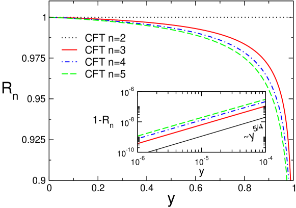
Figure 2: Scaling function $R_{n}(y)$ (CFT prediction) for the 1D Ising universality class. We show $R_{n}(y)$ as a function of the harmonic ratio $y$ for $n=2,3,4,5$. The inset is to highlight the small $y$ behavior of $R_{n}(y)$. The continuous black line is $\sim y^{5/4}$.

and ${}_{2}F_{1}$ is the hypergeometric function. Notice that for $n=2$ (25) can be expressed in terms of elementary functions as [21]

$${\cal F}_{2}(x)=\frac{1}{\sqrt{2}}\Bigg{[}\left(\frac{(1+\sqrt{x})(1+\sqrt{1-x})}{2}\right)^{1/2}+x^{1/4}+((1-x)x)^{1/4}+(1-x)^{1/4}\Bigg{]}^{1/2}$$ (29)

The exact analytic form of $R_{n}(y)$ in the Ising universality class is obtained from (25) and (23). This is shown numerically in Fig. 2 ($R_{n}(y)$ as a function of the harmonic ratio $y$ for $n=2,3,4,5$). Clearly $R_{n}(y)$ (for any $n$) is very close to one in the region $y\sim 0$ and is monotonically vanishing in the limit $y\to 1$. Note that $R_{2}(y)$ is exactly one ($R_{2}=1$ $\forall y$). The asymptotic behavior of $R_{n}(y)$ in the limit $y\to 1$, when the two intervals are next to each other (cf. Fig. 1), is given by (24). For instance, for $n=3,4$ one has $R_{3}(y)\sim(1-y)^{1/9}$ and $R_{4}(y)\sim(1-y)^{1/8}$, which explains the slowly vanishing behavior observed in Figure 2.

Oppositely, in the limit $y\to 0$, when the two intervals are very far apart ($d\gg 1$ in Fig. 1), the same asymptotic behavior, $R_{n}(y)\sim 1-\alpha_{n}y^{5/4}$, for all the values of $n>2$ is observed (this is highlighted in Fig. 2: Inset). In principle the exponent $5/4$ could be calculated analytically using the same methods employed in Ref. [17] to obtain the small $y$ expansion of ${\cal F}_{n}(y)$. Note that one should expect $\alpha_{n}\to 0$ in the limit $n\to 1$, reflecting that the negativity vanishes faster than any power at $y\to 0$ [32, 33].

4 The universal ratio $R_{n}$ in the free compactified boson theory

In this section we re-derive (for more details cf. [33]) the asymptotic scaling function $R_{n}(y)$ for a free compactified boson theory. This is defined by the field theory action

$$S=\frac{1}{2\pi}\int dzd\bar{z}\partial\phi\bar{\partial}\phi$$ (30)

where $\phi$ are bosonic fields compactified on a circle of radius $r_{circle}$, meaning that $\phi=\phi+2\pi r_{circle}$. The action (30) is also the so-called Luttinger liquid, which is a $c=1$ CFT and one of the most successful paradigms to understand the physics of 1D systems. For instance the theory describes the critical long wavelength behavior of the anisotropic Heisenberg spin chain in its gapless phase, bosons with repulsive delta interaction, 1D Hubbard model, etc..

For the free compactified boson theory (30) the scaling function ${\cal F}_{n}(x)$ has been calculated in Ref. [16] and is given as

$$\mathcal{F}_{n}(x)=\frac{\Theta\big{(}{\bf 0}|\eta\Gamma\big{)}\,\Theta\big{(}{\bf 0}|\Gamma/\eta\big{)}}{[\Theta\big{(}{\bf 0}|\Gamma\big{)}]^{2}}$$ (31)

where $\Theta$ and $\Gamma$ are the same as for the Ising universality class (cf. previous section). Here $\eta$ is related to the compactification radius $r_{circle}$ as $\eta=2r^{2}_{circle}$ and can be also given in terms of the so-called Luttinger liquid parameter $K_{L}$ as $\eta=1/(2K_{L})$. For $n=2$ (31) is expressed in terms of the Jacobi theta functions $\theta_{\nu}$ as [14]

$${\cal F}_{2}(y)=\frac{\theta_{3}(\eta\tau)\theta_{3}(\tau/\eta)}{[\theta_{3}(\tau)]^{2}}$$ (32)

where $\tau$ is related to the harmonic ratio as $y=[\theta_{2}(\tau)/\theta_{3}(\tau)]^{4}$. Notice in both (31)(32) the explicit invariance under $\eta\to 1/\eta$. The point $\eta=4$ ($r_{circle}=\sqrt{2}$) describes the critical behavior of the 2D XY model at the BKT transition (or equivalently the long wavelength properties of the 1D Heisenberg XXZ chain at anisotropy $\Delta=-1/\sqrt{2}$) (cf. [36]).

Figure 3: (a) Scaling function $R_{n}(y)$ for the free compactified boson theory at $\eta=4$ ($r_{circle}=\sqrt{2}$). CFT prediction versus the harmonic ratio $y$ for $n=2,3,4,5$. For each $n$ the CFT result for the free boson in the decompactified limit (i.e. at $\eta=\infty$) is also shown (rhombi). Inset: small $y$ behavior of $R_{n}(y)$, plot of $1-R_{n}(y)$ versus $y$. The continuous black line is $\sim y^{5/4}$. (b) $R_{n}(y)$ ($n=3,4,5$) at fixed $y=1/2$ as a function of $\eta=2r^{2}_{circle}$.

Before proceeding one should remark that (31) is only defined for positive values of its argument $x$. Since in (23) the combination $y/(y-1)$ is negative for $y\in[0,1)$, one should consider the analytic continuation for negative argument of (31). This has been calculated in Ref. [33] and is given as

$${\mathcal{F}}_{n}(y)=\frac{\eta^{\frac{n-1}{2}}\Theta\Big{(}{\bf 0}|\eta\,G\big{[}y/(y-1)\big{]}\Big{)}}{\sqrt{\prod\limits_{k=1}^{n-1}\textrm{Re}(F_{k/n}(\frac{y}{y-1})\bar{F}_{k/n}(\frac{1}{1-y}))}}$$ (33)

where $F_{q}(x)\equiv_{2}F_{1}(q,1-q,1,x)$ and we defined $G$ as

$$G\equiv 2i\left(\begin{array}[]{cc}A&W\\ W^{T}&B\end{array}\right)$$ (34)

The matrix elements of $G$ are given as

$$A=\sum\limits_{k=1}^{n-1}\frac{|\tau_{k/n}|^{2}}{\beta_{k/n}}\sin(\pi k/n)E_{k/n}\qquad B=\sum\limits_{k=1}^{n-1}\frac{1}{\beta_{k/n}}\sin(\pi k/n)E_{k/n}$$ (35)

$$W=-\sum\limits_{k=1}^{n-1}\frac{\alpha_{k/n}}{\beta_{k/n}}\sin(\pi k/n)[\sin(\pi k/n)-i\cos(\pi k/n)]E_{k/n}$$

where we used the definitions

$$\tau_{k/n}=i\frac{F_{k/n}(1-x)}{F_{k/n}(x)}\equiv\alpha_{k/n}+i\beta_{k/n},\qquad(E_{k/n})_{rs}\equiv e^{2\pi ik/n(r-s)}/n$$ (36)

The ratio $R_{n}(y)$ can now be obtained using (33) and (23). This is shown numerically in Fig. 3 (a) plotting $R_{n}(y)$ as a function of $y$ for $n=2,3,4,5$. The form of $R_{n}(y)$ is very similar to the Ising case (Fig. 2). Precisely, $R_{n}(y)\approx 1$ in the whole region $0\leq y\lesssim 1$, while in the limit $y\to 1$ $R_{n}(y)$ vanishes (faster than in the Ising case due to the larger value of the central charge, cf. (24)). Note, however, that $R_{n}(y)$ ranges in a larger interval compared to the Ising case: for instance it is $0.9\lesssim R_{3}(y)\leq 1$ for $0\leq y\lesssim 3/4$, while in the same region one has $0.98\lesssim R_{3}(y)\leq 1$ for the Ising (cf. Fig. 2).

Remarkably, the same asymptotic behavior $R_{n}(y)\sim 1-\alpha^{\prime}_{n}y^{5/4}$, as in the Ising case, is shown in the limit $y\to 0$ (Fig. 3: Inset). Also it should be $\alpha^{\prime}_{n}\to 0$ at $n\to 1$ (as proven analytically in [33] for arbitrary values of the compactification radius).

Interestingly, $R_{n}(y)$ depends weakly on the compactification radius $r_{circle}$, hence on $\eta$. For example in the range $2\lesssim\eta\leq\infty$, with $\eta=\infty$ the so-called decompactified limit, $R_{n}(y)$ does not change significantly as a function of $y$ (in Fig. 3 the difference between $\eta=\infty$ and $\eta=4$ is not visible at all). This is better highlighted in Fig. 3 (b) showing $R_{n}(y)$ at fixed $y=1/2$ as a function of $\eta=2r^{2}_{circle}$. Notice that, since $R_{n}(y)$ inherits the symmetry under $\eta\to 1/\eta$ from the ${\cal F}_{n}(y)$ (cf. (31)), one has $R_{n}(\eta)=R_{n}(1/\eta)\,\forall(y,n)$. In Fig. 3 for each $n$ $R_{n}(y)$ exhibits a minimum at $\eta=1$, which corresponds to the antiferromagnetic Heisenberg XXX model, while in the region $\eta>1$ it increases monotonically showing a saturating behavior for large $\eta$. In particular already for $\eta\gtrsim 2$ $R_{n}(y)$ cannot be distinguished from its asymptotic value. The same weak dependence on $\eta$ is observed at other values of $y$. One must mention that it is possible to calculate $R_{n}(y)$ directly in the decompactified limit (i.e. $\eta\to\infty$) using (33) (cf. Ref. [32] for the analytic result).

5 The moments of $\rho_{A}^{T_{2}}$ in Monte Carlo simulations

In this section we present a Monte Carlo scheme for calculating $\Tr(\rho_{A_{1}\cup A_{2}}^{T_{2}})^{n}$ using the replica trick and classical Monte Carlo simulations. This is based on the approach developed in [15, 21, 22] for $\Tr\rho_{A}^{n}$ (Rényi entropies) and can be in principle applied to any model that can be simulated with classical Monte Carlo. The method employs the mapping between a quantum system in $d$ dimensions and a classical one living in $d+1$. We should mention that an alternative numerical approach for calculating both $\Tr(\rho_{A}^{T_{2}})^{n}$ and ${\cal E}$ using TTN (tree tensor network) techniques [46, 47, 48, 49, 50, 51, 52, 53, 54, 55, 56, 57, 58] has become available recently [44].

The section is organized as follows. We first review in 5.1 the replica representation for the moments of both $\rho_{A}$ and $\rho_{A}^{T_{2}}$, which lies at the heart of the method. The moments can be measured in Monte Carlo simulations using the strategy outlined in 5.2. Finally, in 5.3 we provide an improved scheme for models admitting a representation in terms of cluster variables.

5.1 Replica trick

The partition function $Z=\Tr e^{-\beta H}$ of a $d$-dimensional quantum system (defined in terms of an Hamiltonian $H$) at inverse temperature $\beta$ can be written as an Euclidean path integral in $d+1$ dimensions as

$$Z=\int{\cal D}[\phi]e^{-S(\{\phi\})}$$ (37)

where $\phi(\vec{x},\tau)$ is a field living on the hypercubic lattice $\{\vec{x},\tau\}$ and $S$ the Euclidean action. The spatial coordinates $x_{i}$ are such that $0\leq x_{i}<L_{i}$ with $i=1,2,\dots,d$ and the imaginary time $\tau$ ranges in the interval $0\leq\tau<L_{\tau}=\beta$. The fields $\phi$ are periodic along the imaginary time direction, i.e. $\phi(\vec{x},\tau+\beta)=\phi(\vec{x},\tau)$.

Here we consider the $n-$th ($n\in{\mathbb{N}}$) power of the partition function (or the replicated partition function) which reads

$$Z^{n}=\int\prod\limits_{k=1}^{n}{\cal D}[\phi_{k}]e^{-\sum\limits_{k=1}^{n}S(\{\phi_{k}\})}$$ (38)

where $\phi_{k}\equiv\phi_{k}(\vec{x},\tau)$ is now a field living on the $k$-th replica and $S(\phi_{k})$ is the replica Euclidean action. The actual form of the action $S$ is not important for the following, but for the sake of simplicity we restrict to the case of nearest-neighbor interactions (which include the models treated in this work) and we consider $1+1$ dimensions. Thus we assume that the action $S$ (defined on the $k-$th replica) is of the form

$$S(\phi_{k})=\sum\limits_{\langle ij\rangle}F(\phi_{k}(i),\phi_{k}(j))$$ (39)

where $\langle ij\rangle$ denotes nearest-neighbor sites and the function $F$ models the interaction between the fields $\phi$. Since we consider periodic spin chains (see Fig. 1) we assume on each replica periodic boundary conditions also along the spatial direction.

5.1.1 Replica representation for the moments of $\rho_{A}$ (Rényi entropies).

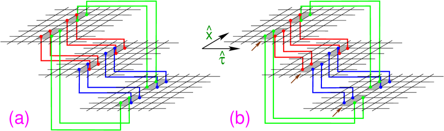
Figure 4: Lattice version of the $n-$sheeted Riemann surface ${\mathcal{R}}_{n}$ (see (a)) and the surface (see (b)) ${\mathcal{K}}_{n}$ obtained sewing together $n=3$ independent replicas. On each replica $\hat{x}$ and $\hat{\tau}$ stand respectively for the spatial and imaginary time directions. The shadow is to highlight the position of the cut, while colored links connect points on different replicas. We show the case of two disjoint intervals of lengths $\ell_{1}=\ell_{2}=2$ at distance $d=1$. In (a) (b) in each replica (plane) periodic boundary conditions on both sides are assumed and the partial transposition is done with respect to the degrees of freedom living on the cuts in front (marked by the arrows in (b)).

We recall that the moments of the reduced density matrix $\Tr\rho_{A}^{n}$ can be obtained considering the Euclidean partition function over the so called $n$-sheeted Riemann surface ${\cal R}_{n}$ (see [6, 4]). In order to define ${\cal R}_{n}$ we restrict for the moment to the case of $A$ being a single interval. Let us start with the set of $n$ independent replicas (sheets). Given the sheet (of area $L\times L_{\tau}$) corresponding to each replica, we consider two points of its dual lattice lying along the spatial direction (these would correspond to the endpoints of subsystem A). Then we define a “cut” $\lambda$ as the straight line joining the two points, its length being the length of subsystem $A$. The $n-$sheeted Riemann surface is defined by assuming that all the links starting from points on the $k-$th replica and intersecting the cut connect to points on the replica $k+1(\textrm{mod}\,n)$.

The generalization of ${\cal R}_{n}$ to multi intervals is done in the straightforward way. As an example in Fig. 4 (a) we show the $3-$sheeted Riemann surface with $L=L_{\tau}=7$ and $\lambda$ made of two disjoint intervals of equal length $\ell=2$ at distance $d=1$.

We now introduce the coupled action $S^{(n)}$ over the $n-$sheeted Riemann surface as

$$S^{(n)}(\{\phi_{k}\})=\sum\limits_{k=1}^{n}\sum_{\langle ij\rangle\nrightarrow\lambda}F(\phi_{k}(i),\phi_{k}(j))+\sum\limits_{\langle ij\rangle\rightarrow\lambda}F(\phi_{k}(i),\phi_{k+1(mod\,n)}(j))$$ (40)

where $\langle ij\rangle\rightarrow\lambda$ ($\langle ij\rangle\nrightarrow\lambda$) denotes the links which (do not) cross the cut $\lambda$. Defining as $Z_{n}[\lambda]\equiv\int\prod_{k}{\cal D}[\phi_{k}]e^{-S^{(n)}(\{\phi_{k}\})}$ the partition function obtained from (40), finally $\Tr\rho^{n}_{A}$ is given by [3]

$$\Tr\rho^{n}_{A}=\frac{Z_{n}[\lambda]}{Z^{n}}$$ (41)

which is formula (12) introduced in section 2. As a final remark one should stress that, in order to recover $\Tr\rho_{A}^{n}$ for the one dimensional quantum system, the limit $L_{\tau}=\beta\to\infty$ has to be taken. In actual Monte Carlo simulations, however, it is sufficient to consider very elongated lattices with $L\ll L_{\tau}$ .

5.1.2 Replica representation for the moments of $\rho_{A}^{T_{2}}$.

A representation similar to (41) can be obtained for the moments $\Tr(\rho_{A}^{T_{2}})^{n}$. To this purpose we consider a slight modification of action (40). Now one has $A=A_{1}\cup A_{2}$, the partial transposition being done with respect to the degrees of freedom of subsystem $A_{2}$. The cut $\lambda$ is made of two segments as $\lambda=\lambda_{1}\cup\lambda_{2}$, with $\lambda_{1},\lambda_{2}$ referring respectively to block $A_{1}$ and $A_{2}$. The modified action reads

$$S^{(n,T_{2})}(\{\phi_{k}\})=\sum\limits_{k=1}^{n}\sum\limits_{\langle ij\rangle\nrightarrow\lambda_{1}\cup\lambda_{2}}F(\phi_{k}(i),\phi_{k}(j))+$$ (42)

$$\sum\limits_{\langle ij\rangle\rightarrow\lambda_{1}}F(\phi_{k}(i),\phi_{k+1({mod}\,n)}(j))+\sum\limits_{\langle ij\rangle\rightarrow\lambda_{2}}F(\phi_{k}(i),\phi_{k-1({mod}\,n)}(j))$$

Notice that in (42) the links crossing $\lambda_{1}$ and $\lambda_{2}$ connect fields living respectively on the replicas $k,k+1(\textrm{mod}\,n)$ and $k,k-1(\textrm{mod}\,n)$, which can be seen as the net effect of the partial transposition. The geometric object (that we call ${\cal K}_{n}$) over which (42) is defined is not the $n-$sheeted Riemann surface, but in general has a different topology. For the case $n=3$ and two intervals of length $\ell_{1}=\ell_{2}=2$ at distance $d=1$ this is depicted in Fig. 4 (b).

After defining the partition function obtained from the action  (42) as $Z^{T_{2}}_{n}[\lambda]$ one has [32, 33]

$$\Tr(\rho_{A}^{T_{2}})^{n}=\frac{Z^{T_{2}}_{n}[\lambda]}{Z^{n}}$$ (43)

which is the analog of (41). Both (41) and (43) can be calculated efficiently in Monte Carlo simulations.

5.2 Measuring the moments of $\rho_{A}^{T_{2}}$ in Monte Carlo simulations

In this section we show how to calculate in Monte Carlo simulations the ratio of partition functions (43) (with minor changes the same strategy applies to (41)). We start with defining the operator

$${\mathcal{O}}\equiv\exp\left[-S_{\lambda}^{(n,T_{2})}(\phi_{1},\phi_{2},\dots,\phi_{n})+\sum_{k}S_{\lambda}(\phi_{k})\right]$$ (44)

where $S_{\lambda}$ and $S^{(n,T_{2})}_{\lambda}$ are the “cut-linked” actions obtained by considering respectively in (40) (42) only the terms with $\langle ij\rangle$ crossing the cut $\lambda$. Then, by definition one has

$$\langle{\mathcal{O}}\rangle=\Tr(\rho_{A}^{T_{2}})^{n}=\frac{Z^{T_{2}}_{n}[\lambda]}{Z^{n}}$$ (45)

where $\langle\cdot\rangle$ stands for the Monte Carlo average over the fields configurations $\{\phi_{k}(\vec{x},\tau)\}$. These are sampled in the Monte Carlo according to the Boltzmann weights $e^{-\sum_{k}S(\phi_{k})}$ constructed from the uncoupled action (39).

At this point an important remark is in order: although the direct implementation of (44) in simulations is legitimate, its typical Monte Carlo history shows a huge variance, due to the presence of the exponential in the definition of ${\cal O}$. This makes (44) not useful in practice.

5.2.1 The increment trick.

A better behaving observable, which allows to overcome this issue, is obtained splitting the cut $\lambda$ in $s$ smaller parts $\lambda^{(i)}$ such that $\lambda\equiv\bigcup_{i=1}^{s}\lambda^{(i)}$ and $s$ is chosen arbitrarily. Defining $\hat{\lambda}^{(i)}\equiv\bigcup_{k=1}^{i}\lambda^{(k)}$ one has the trivial identity

$$\frac{Z_{n}^{T_{2}}[\lambda]}{Z^{n}}=\prod\limits_{i=0}^{s}\frac{Z_{n}^{T_{2}}[\hat{\lambda}^{(i+1)}]}{Z_{n}^{T_{2}}[\hat{\lambda}^{(i)}]}$$ (46)

For each term in the product in (46) one can now write

$$\langle\widetilde{\mathcal{O}}\rangle_{\lambda^{\prime}}\equiv\frac{Z_{n}^{T_{2}}[\hat{\lambda}^{(i+1)}]}{Z_{n}^{T_{2}}[\hat{\lambda}^{(i)}]}$$ (47)

where the modified observable $\widetilde{\mathcal{O}}$ is defined as

$$\widetilde{\mathcal{O}}\equiv\exp\left[S_{\lambda^{\prime}}^{(n,T_{2})}-S^{(n,T_{2})}_{\lambda^{\prime\prime}}\right]$$ (48)

with $\lambda^{\prime\prime}\equiv\hat{\lambda}^{(i+1)}$ and $\lambda^{\prime}\equiv\hat{\lambda}^{(i)}$. The Monte Carlo average in (47) is taken with respect to the action $S^{(n,T_{2})}$ with cut $\lambda^{\prime}$. Now (48) receives contribution only from “fluctuations” living on a portion of the cut and its variance, compared to the one of (44), is strongly reduced.

Further improvements are possible if the model considered (defined by the Euclidean action $S$) admits a representation in terms of clusters [59, 60] (à la Fortuin-Kasteleyn) and can be simulated using a Swendsen-Wang like algorithm [61]. Then it is convenient to express (48) in terms of cluster-related quantities. It turns out that since clusters are non local objects this improves dramatically the efficiency of the procedure highlighted so far.

5.3 Improved Monte Carlo scheme via the “cut-linked” cluster representation

In this section we describe the improved Monte Carlo method to simulate $\Tr(\rho_{A}^{T_{2}})^{n}$ (and $\Tr\rho_{A}^{n}$) for models that admit a representation in terms of clusters. We restrict to the case of 2D square lattices, although the method can be extended to models defined on arbitrary graphs and any dimension in a straightforward way. We first introduce the so called random cluster model [59].

Let us consider a square lattice and denote with $e$ a generic edge (or link) connecting two nearest-neighbor sites $x,y$. Let us also define $E$ as the set of all the links on the lattice and for each $e\in E$ consider a “link function” $\omega(e)$ such that $\omega(e)\to\{0,1\}$. We call a link $e$ active (inactive) if $\omega(e)=1$ ($\omega(e)=0$), while the set of all the possible link configurations is $\Omega$ (i.e. $\Omega\equiv\{0,1\}^{E}$). Given an element $\gamma\in\Omega$ we also consider the set of the active links ${\cal C}_{\gamma}\equiv\{e\in E:\omega(e)=1\}$. Finally, the clusters in the configuration $\gamma$ are defined as the connected components of ${\cal C}_{\gamma}$.

The random cluster model, which depends on the two parameters $p$ (probability of activating a link) and $q$ (cluster weight), is defined through the partition function

$$Z=\sum\limits_{\gamma\in\Omega}\left\{\prod\limits_{e\in E}p^{\omega(e)}(1-p)^{1-\omega(e)}\right\}q^{k(\gamma)}$$ (49)

where we denote with $k(\gamma)$ the “counting function” giving the total number of clusters in $\gamma$. Many models in statistical mechanics can be mapped to the random cluster model (Ising, Potts models, percolation models are just few well known examples). For instance (49) becomes the partition function of the 2D Ising model if one chooses

$$q=2\quad p=1-e^{-\beta J}$$ (50)

with $\beta$ as usual the inverse temperature.

Clearly, the definition of the random cluster model can be extended to the surface ${\cal K}_{n}$ (or to the $n$-sheeted Riemann surface ${\cal R}_{n}$) in a straightforward way. To this purpose we first observe that the set of all the possible links configurations does not depend on the presence of the cut $\lambda$ (since the total number of links is not affected by the geometry of the surface) and is given as $\Omega_{{\cal K}_{n}}=\Omega^{n}=\{0,1\}^{nE}$. Thus the partition function of the random cluster model on ${\cal K}_{n}$ (i.e. $Z_{n}^{T_{2}}[\lambda]$) reads

$$Z_{n}^{T_{2}}[\lambda]=\sum\limits_{\gamma\in\Omega^{n}}\left\{\prod\limits_{e\in E}p^{\omega(e)}(1-p)^{1-\omega(e)}\right\}q^{k_{\lambda}(\gamma)}$$ (51)

where $k_{\lambda}(\gamma)$ is the same counting function as in (49). The subscript $\lambda$ is to stress that for a given $\gamma$ the number of clusters depends on the cut (and hence on the geometry of the surface), i.e. it can be $k_{\lambda}(\gamma)\neq k_{\lambda^{\prime}}(\gamma)$ if $\lambda\neq\lambda^{\prime}$.

In order to derive the (“improved”) cluster version of (48) we observe that the partition function of the random cluster model on the surface ${\cal K}_{n}$ with a different cut $\lambda^{\prime}$ formally can be obtained from (51) (with cut $\lambda$) as

$$Z_{n}^{T_{2}}[\lambda^{\prime}]=\sum\limits_{\gamma\in\Omega^{n}}\left\{\prod\limits_{e\in E}p^{\omega(e)}(1-p)^{1-\omega(e)}\right\}q^{k_{\lambda}(\gamma)-k_{\lambda}(\gamma)+k_{\lambda^{\prime}}(\gamma)}$$ (52)

In writing (52) we used that, for each fixed $\gamma$, the term in the curly brackets does not depend on the cut. Dividing (52) by $Z_{n}^{T_{2}}[\lambda]$ we obtain the elegant result

$$\frac{Z_{n}^{T_{2}}[\lambda^{\prime}]}{Z_{n}^{T_{2}}[\lambda]}=\langle q^{-k_{\lambda}+k_{\lambda^{\prime}}}\rangle_{\lambda}$$ (53)

where the average $\langle\cdot\rangle_{\lambda}$ is done (as the subscript stresses) using the action defined on the surface ${\cal K}_{n}$ with cut $\lambda$. Finally, the cluster representation of (48) is given by

$$\widetilde{\mathcal{O}}=q^{k_{\lambda^{\prime}}-k_{\lambda}}$$ (54)

with the choice $\lambda=\hat{\lambda}^{(i)}$ and $\lambda^{\prime}=\hat{\lambda}^{(i+1)}$. An important property, which is useful in Monte Carlo simulations to speed up the evaluation of the average in (53), is that the difference $k_{\lambda^{\prime}}-k_{\lambda}$ depends only on the clusters “intersecting” the portion of the cut $\lambda\cup\lambda^{\prime}-\lambda\cap\lambda^{\prime}$ (i.e. only on the “cut-linked” clusters), while other contributions trivially cancel.

6 Monte Carlo results: Ising universality class

In this section we numerically investigate the properties of the scale invariant ratios $r_{n}$ and $R_{n}$ in the 1D quantum Ising universality class. The Monte Carlo data that we present have been obtained using the results in section 5, i.e. simulating the 2D Ising model at the critical point $\beta_{c}\equiv 1/T_{c}=1/2\log(1+\sqrt{2})$. In particular we used the improved scheme described in 5.3 (details about the simulations can be found in A).

6.1 Two adjacent intervals: the ratios $r_{n}$

Let us consider two adjacent intervals $A_{1},A_{2}$ of equal length $\ell$ (this corresponds to the situation shown in Fig. 1 (b)). In Fig. 5 we show Monte Carlo data for $r_{3}$ $r_{4}$ as a function of $z\equiv\ell/L$. We considered in our simulations only $L=50,100,150$ and $1\leq\ell\leq L/2$. The asymptotic behavior $r_{n}(z)$ has been obtained analytically in CFT for any $n$ in Ref. [32]. This is given in terms of (18) (cf. section 2) after replacing $\ell\to L/\pi\sin(\pi\ell/L)$. The result is reported in Fig. 5 with the dashed-dotted line.

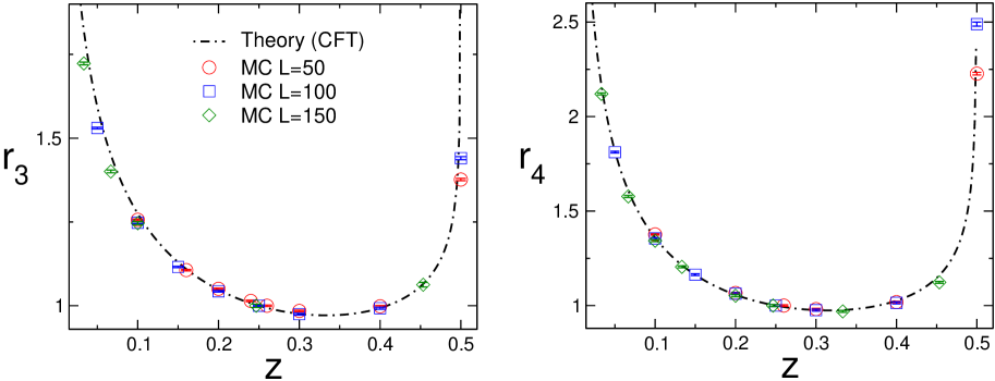
Figure 5: The ratios $r_{3}$ (left) and $r_{4}$ (right) versus $z\equiv\ell/L$ in the 2D classical critical Ising model. Monte Carlo data for several values of $L=50,100,150$. The dashed dotted line is the CFT prediction (no fitting parameters). For all the data Monte Carlo errors are smaller than the symbols.

Monte Carlo data show data collapse for both $r_{3},r_{4}$ and for all the values of $L,\ell$ simulated, supporting scale invariance (although this is expected only in the asymptotic limit $L,\ell\to\infty$). Also, the behavior of the data is perfectly reproduced by the CFT result. Deviations from the theory are only visible in the regions $z\sim 0$ and $z\sim 1/2$. These are understood as finite (interval) size effects. Indeed for small $z$ very large system sizes are needed to reach the asymptotic limit where CFT holds. For instance, $z=0.05$ and $L=150$ (which is the largest system size we simulated) corresponds to block size $\ell=zL=7.5$, which is apparently too small and far from the scaling limit. Similar corrections have been observed for $r_{3},r_{4}$ in free bosonic systems (harmonic chain) [32, 33] (cf. also [44] for recent results in the Ising chain using TTN techniques).

6.2 Two disjoint intervals: the ratio $R_{3}$

We now discuss the case of two disjoint intervals (geometry in Fig. 1 (c)) focusing on the behavior of the ratios $R_{n}(y)$ (we restrict to $n=3$). We first remind that for any $n$, in the limit $L,\ell\to\infty$, $R_{n}(y)$ are universal functions of the harmonic ratio $y$, and in a CFT are given by (22) (cf. section 3 for the analytical results in the Ising case).

In Fig. 6 (top) we show Monte Carlo data for $R_{3}(y)$ for several values of the harmonic ratio $0\leq y\leq 1$ and $L=80,120,160$ (data at fixed $\ell=20$). Data at different $y$ are obtained varying the distance between the two intervals (according to formula (5)).

Remarkably, all the data for different sizes $L$ collapse on the same curve within the Monte Carlo statistical error, meaning that finite $L$ scaling corrections are not visible. Nonetheless, at finite $\ell=20$ Monte Carlo data do not match the theoretical (CFT) curve (dashed-dotted line), suggesting that finite $\ell$ corrections are present. The CFT result is only recovered in the limit $\ell\to\infty$. General renormalization group arguments suggest the behavior

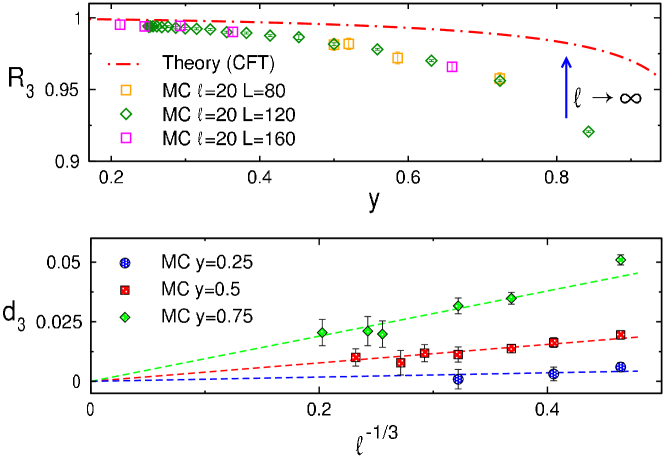
Figure 6: Unusual scaling corrections for the ratio $R_{3}(y)$ in the Ising universality class. (top) $R_{3}(y)$ as a function of the harmonic ratio $y$ (Monte Carlo data for two disjoint intervals of length $\ell=20$ and total system sizes $L=80,120,160$). Different values of $y$ are obtained varying the distance between the two intervals. The CFT prediction (dashed dotted line) is recovered in the asymptotic limit (i.e. $\ell\to\infty$), as stressed by the vertical arrow. (bottom) Plot of $d_{3}(y)\equiv R^{CFT}_{3}(y)-R_{3}(y)$ versus $\ell^{-1/3}$. Monte Carlo data at fixed $y=0.25,0.5,0.75$ and $10\leq\ell\leq 120$. The dashed lines is the fit to $d_{3}=a_{0}\ell^{-1/3}$ with $a_{0}$ the only fitting parameter. In both plots the Monte Carlo statistical error bar is often smaller than the symbols.

$$R_{n}(y)=R^{CFT}_{n}(y)+\ell^{-\omega_{n}}a_{n}(y)+\cdots$$ (55)

with $R_{n}^{CFT}(y)$ the asymptotic scaling function given by formula (22), while $\omega_{n}$ and $a_{n}(y)$ are respectively the exponent and amplitude of the scaling corrections. The dots in (55) denote more irrelevant terms. Note in (55) the dependence of $a_{n}$ on the harmonic ratio $y$. The very same behavior (upon replacing $R_{n}(y)\to{\cal F}_{n}(y)$ in (55) and fixing $\omega_{n}=1/n$) is shown by the scaling corrections of the mutual information [14, 15, 16, 18, 19, 21, 22, 24, 25, 26, 27, 17, 23].

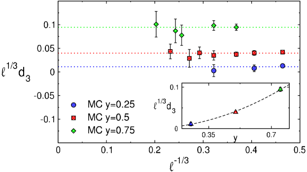
Figure 7: Amplitude $a_{3}(y)$ of the unusual corrections extracted as $a_{3}(y)=\ell^{1/3}d_{3}(y)$ with $d_{3}$ defined as in Fig. 6. Same Monte Carlo data as in Fig. 6 at fixed $y=1/4,1/2,3/4$. We plot $a_{3}\equiv\ell^{1/3}d_{3}(y)$ versus $\ell^{-1/3}$. The dotted lines are fits to a constant. Inset: fitted values for $a_{3}$ (dotted lines in the main Figure) plotted versus $y$. The dashed line is a fit to $Ay^{2}$.

More generally, entanglement related quantities are known to exhibit unusual scaling corrections. These are induced by the presence of the conical singularities (at the edges of the subsystem) needed to write the reduced density matrix (and the partially transposed one) in the quantum field theory language [10].

At difference with usual corrections, arising due to the presence of irrelevant (in the renormalization group sense) operators in the theory, the unusual ones are induced by a local insertion, near the conical singularity, of an operator that would be relevant in the bulk. The scaling dimension $x$ of the operator determines the exponent of the unusual corrections as $\omega_{n}=2x/n$. For this reason the analysis of entanglement corrections provides a tool to unveil universal information about critical systems.

On the other hand, it is a hard task in general to identify the relevant operator inducing the unusual corrections because any operator which does not break the symmetries of the model is in principle allowed [10]. For the Ising universality class it has been shown that this is the Majorana operator (with $x=1/2$), implying $\omega_{n}=1/n$. It is natural to expect that the same one induces the scaling corrections of $R_{n}(y)$, although their exponent could be different (i.e. $\omega_{n}\neq 1/n$).

To clarify this issue in Fig. 6 (bottom) we show $d_{3}(y)\equiv R_{3}^{CFT}(y)-R_{3}(y)$ at fixed $y=1/4,1/2,3/4$ and $\ell$ in the range $10\leq\ell\leq 120$. Clearly, Monte Carlo data support the behavior as $\ell^{-1/3}$. We also mention that a fit to $a/\ell^{b}$ leaving $b$ as a free parameter gives the exponent $b=0.4(1)$ again consistent with $b=1/3$. This allows to conclude that in the critical Ising spin chain the unusual corrections for $R_{n}(y)$ are of the same form as the ones for the mutual information.

We provide complementary information about the scaling corrections in Fig. 7, plotting their amplitude $a_{3}(y)$ as a function of $\ell^{-1/3}$. Here $a_{3}(y)$ is extracted from the Monte Carlo data shown in Fig. 6 as $a_{3}(y)=\ell^{1/3}d_{3}(y)$. Its behavior confirms the correctness of the scaling corrections exponent $\omega_{3}=1/3$. A precise estimate for $a_{3}(y)$ is obtained by fitting the data with a constant (dotted lines in the Figure). The results are shown in the inset as a function of the harmonic ratio $y$ and are well described by a parabolic behavior as $\sim y^{2}$ up to $y=3/4$ (dashed line in Fig. 7: Inset). One should stress that this is different from what observed for the mutual information. For instance, it has been shown in Ref. [21] that the amplitude of the corrections to ${\cal F}_{2}(y)$ is very well described by $y^{1/4}$, pointing to a much slower decay in the limit $y\to 0$.

7 Monte Carlo results: 2D XY model at the BKT transition

In this section we numerically investigate the behavior of the ratios $r_{n}$ and $R_{n}$ for the free compactified boson theory with compactification radius $r_{circle}=\sqrt{2}$ (equivalently $\eta=4$ or, in terms of the Luttinger parameter, $K_{L}=2$) [36]. This describes (a part from logarithmic corrections) the critical properties of the 2D classical XY model at the BKT phase transition or, equivalently, the long wavelength behavior of the spin-$\frac{1}{2}$ quantum Heisenberg XXZ chain at anisotropy $\Delta=-1/\sqrt{2}$.

The Monte Carlo data we present have been obtained using the method outlined in 5, simulating the 2D XY model at $\beta_{BKT}$ (for more details about the simulations cf. A). Since for the XY model there is no efficient implementation of the Swendsen-Wang algorithm, we could not use the improved scheme provided in section 5.3.

Nonetheless, one general result of this section is that the scheme described in section 5 is effective for models with continuous degrees of freedom. This is verified in a preliminary step of our analysis (cf. section 7.1) by calculating $\Tr\rho_{A}^{n}$ ($n=2,3,4$ with $A$ a single block) and checking its scaling behavior against the well known CFT result (11).

We then focus (section 7.2) on the ratios $r_{3},r_{4}$ finding that, already for finite intervals, their behavior is well reproduced by the CFT results in Ref. [32, 33]. Surprisingly, this is also the case for the ratio $R_{3}(y)$ for finite (large enough) blocks size, signaling that corrections are smaller than in the Ising case.

7.1 Single interval: the moments of $\rho_{A}$ and the central charge

In this section we validate the Monte Carlo procedure outlined in section 5 for models with continuous degrees of freedom. In particular we discuss Monte Carlo results for the moments $\Tr\rho_{A}^{n}$ ($n=2,3,4$) of the reduced density matrix, demonstrating that their scaling behavior is fully reproduced (as expected) by the CFT result (11). Besides its relevance as a benchmark of the method, our analysis suggests that, even for models defined in terms of continuous variables, entanglement based quantities are effective tools to extract their central charge .

We start with reminding that the scaling behavior of $\Tr\rho^{n}_{A}$ in the asymptotic limit is given in CFT as (cf. section 2)

$$\textrm{Tr}\rho_{A}^{n}\sim c_{n}\left(\frac{L}{\pi}\sin\frac{\pi\ell}{L}\right)^{-\frac{c}{6}(n-\frac{1}{n})}$$ (56)

and $c=1$ for the XY model. In Fig. 8 we show Monte Carlo data for $\textrm{Tr}\rho_{A}^{n}$ with $n=2,3,4$ and $50\leq L\leq 200$, $1\leq\ell\leq 75$. For each $n$ and different $L$ all the data collapse on a single curve meaning that $L$ dependent scaling corrections are not visible within the Monte Carlo error bar.

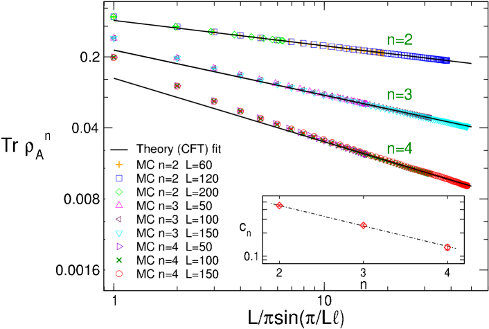
Figure 8: Central charge $c$ of the Berezinskii-Kosterlitz-Thouless universality class (2D XY model at the BKT point $\beta_{BKT}=1.1199(1)$). We show $\textrm{Tr}\rho_{A}^{n}$ (Monte Carlo data) versus $L/\pi\sin(\pi\ell/L)$ for $n=2,3,4$, several values of $L$ $50\leq L\leq 200$, and $1\leq\ell\leq 75$. The Monte Carlo error bar is smaller than the size of the symbols. Continuous lines are one parameter fits to the asymptotic CFT behavior (56) after fixing $c=1$. Inset: Fitted values of the non universal constant $c_{n}$ as a function of $n$ (note the logarithmic scale on the $y$-axis). The dashed line is a fit to an exponential decay.

The continuous (black) lines are given by (56) where we fix the central charge $c=1$, fitting the non universal constant $c_{n}$. For $n=2$ the CFT prediction reproduces the behavior of the MC data in the whole range $1\leq\ell\leq 75$. This is not the case at $n=3,4$ where larger $\ell$ dependent scaling corrections are present and bigger systems are needed in order to reach the asymptotic limit. In fact, agreement with MC data is observed only at $L_{c}\equiv L/\pi\sin(\pi\ell/L)\gtrsim 10$ and $L_{c}\gtrsim 20$ for respectively $n=3,4$. The same increasing trend in the scaling corrections of $\Tr\rho_{A}^{n}$ ( upon increasing the Rényi index $n$) is expected in a generic system described by the Luttinger liquid [8].

To have an independent estimate of the central charge we performed fits leaving $c$ as a free parameter in (56). For $n=2$ a fit to (56) (discarding the data up to $L_{c}\lesssim 8$) gives $c_{2}=0.45(1)$ $c=0.99(1)$ with $\chi^{2}/\textrm{DOF}\approx 1.3$. Similarly for $n=3,4$ one gets respectively $c_{3}=0.25(1)$ $c=1.00(3)$ and $c_{4}=0.13(1)$ $c=1.00(3)$. Finally, in Fig. 8 (inset) we show the fitted value of the non universal constant $c_{n}$ as a function of $n$. Clearly $c_{n}$ shows an exponential decay and is well described by the function $Ae^{-n/n_{0}}$ with $A\approx 1.52$ and $n_{0}\approx 1.64$. Similar exponential behavior of $c_{n}$ has been already observed in the 1D XXZ spin chain [8].

7.2 The ratios $r_{n}$, $R_{n}$

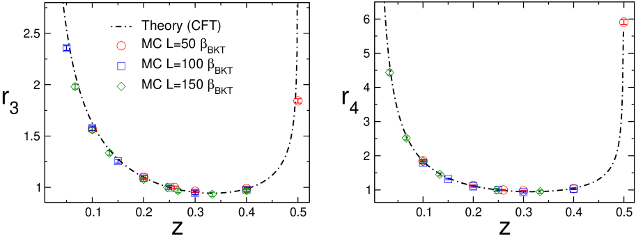
Figure 9: The ratios $r_{3}$ (left) and $r_{4}$ (right) versus $z\equiv\ell/L$ in the 2D XY model at the BKT phase transition. We show Monte Carlo data for several values of $L=50,100,150$. The dashed dotted line is the CFT prediction obtained from (19) (no fitting parameters). For both $r_{3},r_{4}$ the error bar is present although smaller than the symbols.

We now proceed to discuss the behavior of the ratios $r_{n}$. In Fig. 9 we show Monte Carlo data for $r_{3},r_{4}$ versus $z\equiv\ell/L$ and system sizes $L=50,100,150$. We considered $\ell$ in the range $1\leq\ell\leq 75$. As for the Ising universality class Monte Carlo data for different values of $L$ are on the same curve (scale invariance) which is remarkably well described (no fitting parameters) by the CFT result (cf. (19)) (dashed-dotted line in the Figure). Similarly to the Ising case finite size deviations are visible in the regions $z\sim 0,1/2$. Notice also that, due to the larger value of the central charge, both $r_{3}$ $r_{4}$ range in a larger interval, as functions of $z$, compared to Fig. 5.

The behavior of the universal ratio $R_{3}(y)$ is more surprising. Monte Carlo data for $R_{3}(y)$ as a function of the harmonic ratio $y$ are reported in Fig. 10 (data for $\ell=20,40,50$). Focusing on the configuration with $\ell=20,L=120$ Monte Carlo data are in reasonable agreement with the CFT curve (dashed-dotted line) for $y\lesssim 1/2$. Deviations from the theory are visible at $y>1/2$ and increase as a function of $y$, as observed in Ising model (cf. Fig. 6). One striking difference, however, is that apparently they decay faster upon increasing the block size $\ell$, which could suggest a large value of the corrections exponent $\omega_{3}$. This is evident from the perfect match between theory and Monte Carlo for $\ell=40,50$ at respectively $y=1/2$ and $y=3/4$. One should mention, however, that the precision of the data does not allow to extract a reliable estimate of the exponent $\omega_{3}$ and a more careful analysis would be needed to reach a conclusion.

8 Conclusions

Figure 10: Scale invariant ratio $R_{3}(y)$ as a function of the harmonic ratio $y$ (Monte Carlo data for the 2D XY model at the BKT phase transition and $\ell=20,40,50$). The dashed dotted line is the CFT prediction from (33). At fixed $\ell=20,L=120$ different values of $y$ correspond to different distances between the two blocks.

In this work we studied the moments $\Tr(\rho_{A}^{T_{2}})^{n}$ of the partially transposed reduced density matrix $\rho_{A}^{T_{2}}$ in critical quantum spin chains. Given a bipartition of the chains into two parts $A$ and $B$ with $A$ being made of two equal blocks as $A=A_{1}\cup A_{2}$, $\rho_{A}^{T_{2}}$ is obtained from the reduced density matrix $\rho_{A}$ by performing the partial transposition with respect to the degrees of freedom of $A_{2}$. We considered both the situations with two adjacent and disjoint blocks, defining, respectively for the two cases, the ratios $r_{n}$ and $R_{n}(y)$, which are scale invariant at the critical point. Using a new numerical method based on Monte Carlo simulations we characterized their scaling behavior, in the critical Ising spin chain and the 1D anisotropic Heisenberg XXZ model at $\Delta=-1/\sqrt{2}$.

The long wavelength properties of both models are described by well known conformal field theories: the first corresponds in the continuum to a free Majorana fermion (central charge $c=1/2$), while the second is the free compactified boson at compactification radius $r_{circle}=\sqrt{2}$ ($c=1$). In $d+1=2$ dimensions these also correspond respectively to the 2D classical critical Ising model (Ising universality class) and the 2D classical critical XY model (Berezinskii-Kosterlitz-Thouless universality class).

The results of our work can be summarized as follows:

• Exploiting the mapping between a quantum system in $d$ dimensions and a classical one in $d+1$ we developed a new numerical scheme to calculate all the moments of the partially transposed reduced density matrix $\rho_{A}^{T_{2}}$ in classical Monte Carlo simulations. The method generalizes the one used in [15, 21, 22] for calculating the moments of the reduced density matrix $\rho_{A}$ and is effective for systems with both discrete (Ising model) and continuous (XY model) degrees of freedom. For models admitting a representation in terms of cluster variables we provided a modified (improved) version of the algorithm.

• For two adjacent blocks $A_{1},A_{2}$ we studied the behavior (as a function of the length of the two blocks) of the ratio $r_{n}$ (with $n=3,4$) in both the critical Ising quantum spin chain and the 1D anisotropic Heisenberg XXZ model at $\Delta=-1/\sqrt{2}$. In both cases we numerically demonstrated (for the first time in non free models ) that their behavior is well described by CFT (results in Ref. [32, 33]).

• For two disjoint intervals we studied the scaling properties of $R_{3}(y)$, which in the asymptotic limit ($\ell\to\infty$) is a universal function of the harmonic ratio $y$. For the 1D quantum Ising model $R_{3}(y)$ exhibits strong (finite size) unusual scaling corrections [10]. Their exponent $\omega_{3}=1/3$ is the same as that found for the mutual information between the two blocks [21]. After taking into account scaling corrections Monte Carlo data show full agreement with the asymptotic (i.e. for infinite blocks) CFT result. For the XXZ chain, although both usual and unusual corrections are expected, they appear to be much smaller and already for sizes $\ell\sim 50$ we find that $R_{3}(y)$ is in excellent agreement with the theory.

Acknowledgments:

I would like to thank Pasquale Calabrese for drawing to my attention this problem. I would also like to thank Andreas Läuchli and Maurizio Fagotti for collaboration in a related project and interesting discussions. I thank the authors of Ref. [44] for sharing, after this work was completed, their results before publication. This work was partly done during the workshop “New quantum states of matter in and out of equilibrium” at the Galileo Galilei Institute in Florence whose hospitality is gratefully acknowledged. Simulations have been performed on the local cluster at the Max Planck Institute for the Physics of the Complex Systems (MPIPKS) in Dresden.

Appendix A Monte Carlo simulations

A.1 The algorithm

In this appendix we give some details about the Monte Carlo algorithms used for the simulations.

A.1.1 Ising model.

For the simulation of the 2D Ising model we employed the standard implementation of the Swendsen-Wang algorithm as described in [61]. To generate the random numbers needed in the Monte Carlo update we used the Mersenne twister random number generator [63] (the same generator was used for the simulation of the 2D XY model). The cluster labeling step needed in the Monte Carlo update was performed using the standard “ants in the labyrinth” algorithm [64].

A.1.2 XY model.

For the 2D XY model at the BKT point our Monte Carlo algorithm was a local Metropolis update supplemented with some overrelaxation sweeps. The Metropolis update that we used is different from the one usually found in the literature. At each Metropolis step a random vector $\vec{n}=(\cos\alpha,\sin\alpha)$ was chosen with $\alpha$ uniformly distributed in $[0,2\pi]$. Then for each spin $\vec{s}_{x}$ at lattice site $x$ the update proposal $\vec{s}_{x}^{\,\prime}$ was obtained reflecting $\vec{s}_{x}$ with respect to $\vec{n}$, i.e.

$$\vec{s}_{x}^{\,\prime}=2(\vec{n}\cdot\vec{s}_{x})\vec{n}-\vec{s}_{x}$$ (57)

The proposal was accepted with the standard Metropolis probability $\textrm{Min}[e^{-(E-E^{\prime})},1]$ with $E(E^{\prime})$ the energies of the configurations before ad after the update. This procedure allows to avoid the (expensive) evaluation of the exponential function at each site of the lattice (which is the case in the standard Metropolis implementation).

To improve the performances of the Metropolis we added some sweeps of overrelaxation. The proposal for the new configuration $\vec{s}_{x}^{\,\prime}$ in the overrelaxation step is obtained by reflecting $\vec{s}_{x}$ with respect to the local field $\vec{S}=\sum_{y}\vec{s}_{y}$ (the sum is over the nearest neighbor sites of $x$):

$$\vec{s}_{x}^{\,\prime}=2(\vec{s}_{x}\cdot\vec{S})\vec{S}-\vec{s}_{x}$$ (58)

Since the new configuration with $\vec{s}_{x}^{\,\prime}$ has by definition the same energy (as that with $\vec{s}_{x}$) , the update step (58) is accepted with probability one. However, for this reason, overrelaxation is not ergodic and has to be used with some other ergodic algorithm. In our case each Monte Carlo step was a combination of one Metropolis sweep followed by five overrelaxation steps. The overrelaxation sweeps have the advantage that, although the energy does not change, the initial and final configurations can be very different, reducing dramatically the critical slowing down. It can be shown indeed that the autocorrelation time $\tau$ for the 2D XY model at the BKT point, using overrelaxation, can be reduced to $\tau=0.15\xi^{1.2}$ [65] (here $\xi$ is the correlation length) while the standard Metropolis gives $\tau\sim\xi^{2}$. Here it is worth stressing that any non local update (such as the Wolff algorithm [66]) outperforms the procedure outlined above. On the other hand the update scheme that we used is quite effective for frustrated systems where there is no available cluster algorithm [67].

References

References

- [1] L. Amico, R. Fazio, A. Osterloh, and V. Vedral, Entanglement in many-body systems, Rev. Mod. Phys. 80, 517 (2008); J. Eisert, M. Cramer, and M. B. Plenio, Area laws for the entanglement entropy - a review, Rev. Mod. Phys. 82, 277 (2010); P. Calabrese, J. Cardy, and B. Doyon Eds, Entanglement entropy in extended systems, J. Phys. A 42 500301 (2009).
- [2] C. Holzhey, F. Larsen, and F. Wilczek, Geometric and renormalized entropy in conformal field theory, Nucl. Phys. B 424, 443 (1994).
- [3] P. Calabrese and J. Cardy, Entanglement entropy and quantum field theory, J. Stat. Mech. P06002 (2004).
- [4] P. Calabrese and J. Cardy, Entanglement entropy and conformal field theory, J. Phys. A 42, 504005 (2009).
- [5] G. Vidal, J. I. Latorre, E. Rico, and A. Kitaev, Entanglement in quantum critical phenomena, Phys. Rev. Lett. 90, 227902 (2003); J. I. Latorre, E. Rico, and G. Vidal, Ground state entanglement in quantum spin chains, Quant. Inf. Comp. 4, 048 (2004).
- [6] P. Calabrese and J. Cardy, Entanglement entropy and quantum field theory: a non-technical introduction, Int. J. Quant. Inf. 4, 429 (2006).
- [7] J. Cardy, The ubiquitous ’c’: from the Stefan-Boltzmann law to quantum information, J. Stat. Mech. (2010) P10004.
- [8] P. Calabrese, M. Campostrini, F. H. L. Essler, and B. Nienhuis, Parity effects in the scaling of block entanglement in gapless spin chains, Phys. Rev. Lett. 104, 095701 (2010).
- [9] P. Calabrese and F. H. L. Essler, Universal corrections to scaling for block entanglement in spin-1/2 XX chains, J. Stat. Mech. P08029 (2010).
- [10] J. Cardy and P. Calabrese, Unusual corrections to scaling in entanglement entropy, J. Stat. Mech. P04023 (2010).
- [11] P. Calabrese, J. Cardy, and I. Peschel, Corrections to scaling for block entanglement in massive spin-chains, J. Stat. Mech. P09003 (2010).
- [12] J. C. Xavier and F. C. Alcaraz, Rényi Entropy and Parity Effect of the Anisotropic Spin-s Heisenberg Chains with a Magnetic Field, 1103.2103.
- [13] P. Calabrese, M. Mintchev, and E. Vicari, The entanglement entropy of 1D systems in continuous and homogenous space, J. Stat. Mech. P09028 (2011).
- [14] S. Furukawa, V. Pasquier, and J. Shiraishi, Mutual information and compactification radius in a c=1 critical phase in one dimension, Phys. Rev. Lett. 102, 170602 (2009).
- [15] M. Caraglio and F. Gliozzi, Entanglement entropy and twist fields, JHEP 0811: 076 (2008).
- [16] P. Calabrese, J. Cardy, and E. Tonni, Entanglement entropy of two disjoint intervals in conformal field theory, J. Stat. Mech. P11001 (2009).
- [17] P. Calabrese, J. Cardy, and E. Tonni, Entanglement entropy of two disjoint intervals in conformal field theory II, J. Stat. Mech. P01021 (2011).
- [18] H. Casini and M. Huerta, A finite entanglement entropy and the c-theorem, Phys. Lett. B 600 142 (2004); H. Casini, C. D. Fosco, and M. Huerta, Entanglement and alpha entropies for a massive Dirac field in two dimensions, J. Stat. Mech. P05007 (2005); H. Casini and M. Huerta, Remarks on the entanglement entropy for disconnected regions, JHEP 0903: 048 (2009); H. Casini and M. Huerta, Reduced density matrix and internal dynamics for multicomponent regions, Class. Quant. Grav. 26, 185005 (2009); H. Casini, Entropy inequalities from reflection positivity, J. Stat. Mech. P08019 (2010); D. D. Blanco, H. Casini, Entanglement entropy for non-coplanar regions in quantum field theory, Class. Quant. Grav. 28: 215015 (2011);
- [19] P. Facchi, G. Florio, C. Invernizzi, and S. Pascazio, Entanglement of two blocks of spins in the critical Ising model, Phys. Rev. A 78, 052302 (2008).
- [20] S. Ryu and T. Takayanagi, Holographic derivation of entanglement entropy from AdS/CFT, Phys. Rev. Lett. 96, 181602 (2006); S. Ryu and T. Takayanagi, Aspects of holographic entanglement entropy, JHEP 0608: 045 (2006); V. E. Hubeny and M. Rangamani, Holographic entanglement entropy for disconnected regions, JHEP 0803: 006 (2008); M. Headrick and T. Takayanagi, A holographic proof of the strong subadditivity of entanglement entropy, Phys. Rev. D 76, 106013 (2007); T. Nishioka, S. Ryu, and T. Takayanagi, Holographic entanglement entropy: an overview, J. Phys. A 42 (2009) 504008; E. Tonni, Holographic entanglement entropy: near horizon geometry and disconnected regions, JHEP 1105: 004 (2011); A. Allais, E. Tonni, Holographic evolution of the mutual information, JHEP 1201: 102 (2012).
- [21] V. Alba, L. Tagliacozzo, and P. Calabrese, Entanglement entropy of two disjoint blocks in critical Ising models, Phys. Rev. B 81, 060411 (2010).
- [22] V. Alba, L. Tagliacozzo, and P. Calabrese, Entanglement entropy of two disjoint intervals in critical c=1 theories, J. Stat. Mech. P06012 (2011).
- [23] M. Fagotti, New insights in the entanglement of two disjoint blocks, EPL 97 17007 (2012).
- [24] F. Igloi and I. Peschel, On reduced density matrices for disjoint subsystems, EPL 89 40001 (2010).
- [25] M. Fagotti and P. Calabrese, Entanglement entropy of two disjoint blocks in XY chains, J. Stat. Mech. P04016 (2010).
- [26] M. Fagotti and P. Calabrese, Universal parity effects in the entanglement entropy of XX chains with open boundary conditions, J. Stat. Mech. P01017 (2011).
- [27] P. Calabrese, Entanglement entropy in conformal field theory: New results for disconnected regions, J. Stat. Mech. (2010) P09013.
- [28] M. A. Rajabpour and F. Gliozzi, Entanglement entropy of two disjoint intervals from fusion algebra of twist fields, J. Stat. Mech. P02016 (2012).
- [29] J. Cardy, Operator content of two-dimensional conformally invariant theories, Nucl. Phys. B 270 186 (1986); C. Itzykson and J.-B. Zuber, Two-dimensional conformal invariant theories on a torus, Nucl. Phys. B 275 580 (1986); A. Cappelli, C. Itzykson, and J.-B. Zuber, Modular invariant partition functions in two dimensions, Nucl. Phys. B 280 445 (1987); P. Di Francesco, H. Saleur, and J. B. Zuber, Modular invariance in non-minimal two-dimensional conformal theories, Nucl. Phys. B 285 (1987) 454; V. Pasquier, Lattice derivation of modular invariant partition functions on the torus, 1987 J. Phys. A 20, L1229.
- [30] G. Vidal and R. F. Werner, A computable measure of entanglement, Phys. Rev. A 65, 032314 (2002).
- [31] H. Wichterich, J. Molina-Vilaplana, and S. Bose, Scale invariant entanglement at quantum phase transitions, Phys. Rev. A 80, 010304(R) (2009); S. Marcovitch, A. Retzker, M. B. Plenio, and B. Reznik, Critical and noncritical long range entanglement in the Klein-Gordon field, Phys. Rev. A 80, 012325 (2009); H. Wichterich, J. Vidal, and S. Bose, Universality of the negativity in the Lipkin-Meshkov-Glick model, Phys. Rev. A 81, 032311 (2010).
- [32] P. Calabrese, J. Cardy, and E. Tonni, Entanglement negativity in quantum field theory, Phys. Rev. Lett. 109 130502 (2012).
- [33] P. Calabrese, J. Cardy, and E. Tonni, Entanglement negativity in extended systems: A field theoretical approach, J. Stat. Mech. P02008 (2013).
- [34] K. Audenaert, J. Eisert,M. B. Plenio and R. F. Werner, Entanglement Properties of the Harmonic Chain, Phys. Rev. A 66, 042327 (2002).
- [35] F. Gliozzi and L. Tagliacozzo, Entanglement entropy and the complex plane of replicas, J. Stat. Mech. P01002 (2010).
- [36] P. Ginsparg, Applied conformal field theory, in: Les Houches, session XLIX (1988), Fields, strings and critical phenomena, Eds. E. Brézin and J. Zinn-Justin, Elsevier, New York (1989).
- [37] P. Di Francesco, P. Mathieu and D. Senechal, Conformal Field Theory, New York, USA: Springer (1997).
- [38] V. L. Berezinskii, Destruction of Long-range Order in One-dimensional and Two-dimensional Systems having a Continuous Symmetry Group I. Classical Systems, Sov. Phys. JETP 32(3), 493-500 (1971).
- [39] J. M. Kosterlitz and D. J. Thouless, Ordering, metastability and phase transitions in two-dimensional systems, J. Phys. C: Solid State 6 1181 (1973).
- [40] J. M. Kosterlitz, The critical properties of the two-dimensional xy model, J. Phys. C: Solid State Phys. 7 1046 (1974).
- [41] J. V. José, L. P. Kadanoff, S. Kirkpatrick and D. R. Nelson, Renormalization, vortices, and symmetry-breaking perturbations in the two-dimensional planar model, Phys. Rev. B 16, 1217 (1978).
- [42] D. J. Amit, Y. Y. Goldschmidt, and S. Grinstein, Renormalisation group analysis of the phase transition in the 2D Coulomb gas, Sine-Gordon theory and XY-model, J. Phys. A 13 585 (1980).
- [43] M. Hasenbusch and K. Pinn, Computing the roughening transition of Ising and solid-on-solid models by BCSOS model matching, J. Phys. A: Math. Gen. 30 63 (1997). M. Hasenbusch, The two-dimensional XY model at the transition temperature: a high-precision Monte Carlo study, J. Phys. A: Math. Gen. 38 5869 (2005).
- [44] P. Calabrese, L. Tagliacozzo, and E. Tonni, Entanglement negativity in the critical Ising chain, to appear.
- [45] M. B. Hastings, I. Gonzalez, A. B. Kallin, and R. G. Melko Measuring Rényi Entanglement Entropy with Quantum Monte Carlo, Phys. Rev. Lett. 104, 157201 (2010); R. G. Melko, A. B. Kallin, and M. B. Hastings, Finite Size Scaling of Mutual Information: A Scalable Simulation, Phys. Rev. B 82, 100409(R) (2010); R. R. P. Singh, M. B. Hastings, A. B. Kallin, R. G. Melko, Finite Temperature Critical Behavior of Mutual Information, Phys. Rev. Lett. 106, 135701 (2011); S. V. Isakov, M. B. Hastings, R. G. Melko, Topological Entanglement Entropy of a Bose-Hubbard Spin Liquid, Nature Physics 7, 772 (2011); R. K. Kaul, R. G. Melko, A. W. Sandvik, Bridging lattice-scale physics and continuum field theory with quantum Monte Carlo simulations, arXiv:1204.5405 (2012); S. Inglis, R. G.Melko, A Wang-Landau method for calculating Rényi entropies in finite-temperature quantum Monte Carlo simulations, arXiv:1207.5052 (2012); J. Iaconis, S. Inglis, A. B. Kallin, R. G. Melko, Detecting Classical Phase Transitions with Rényi Mutual Information, arXiv:1210.2403 (2012). S. Humeniuk and T. Roscilde, Quantum Monte Carlo calculation of entanglement Rényi entropies for generic quantum systems, Phys. Rev. B 86, 235116 (2012).
- [46] N. Schuch M. M. Wolf, F. Verstraete, and J. I. Cirac, Entropy scaling and simulability by matrix product states, Phys. Rev. Lett. 100, 030504 (2008); D. Perez-Garcia, F. Verstraete, M. M. Wolf, J. I. Cirac, Matrix Product State Representations Quantum Inf. Comput. 7, 401 (2007); L. Tagliacozzo, T. R.de Oliveira, S. Iblisdir, and J. I. Latorre, Scaling of entanglement support for Matrix Product States, Phys. Rev. B 78, 024410 (2008); F. Pollmann, S. Mukerjee, A. M. Turner, and J. E. Moore, Theory of finite-entanglement scaling at one-dimensional quantum critical points, Phys. Rev. Lett. 102, 255701 (2009). J. I. Cirac and F. Verstraete, Renormalization and tensor product states in spin chains and lattices, J. Phys. A 42 (2009) 504004. U. Schollwöck, The density-matrix renormalization group, Rev. Mod. Phys. 77 259 (2005). U. Schollwöck, The density-matrix renormalization group in the age of matrix product states, Ann. Phys. 326, 96 (2011).
- [47] L. Tagliacozzo, G. Evenbly, and G. Vidal, Simulation of two-dimensional quantum systems using a tree tensor network that exploits the entropic area law, Phys. Rev. B 80, 235127 (2009).
- [48] M. Fannes, B. Nachtergaele, and R. F. Werner, Ground states of VBS models on Cayley trees, J. Stat. Phys. 66, 939 (1992).
- [49] B. Friedman, A density matrix renormalization group approach to interacting quantum systems on Cayley trees, J. Phys.: Cond. Matt. 42, 9021 (1997).
- [50] Y. Hieida, K. Okunishi, and Y. Akutsu, Numerical renormalization approach to two-dimensional quantum antiferromagnets with valence-bond-solid type ground state, New J. Phys. 1, 7 (1999).
- [51] M-B. Lepetit, M. Cousy, and G. M. Pastor, Density-matrix renormalization study of the Hubbard model on a Bethe lattice, Eur. Phys. J. B, 13, 421 (2000).
- [52] M. A. Martin-Delgado, J. Rodriguez-Laguna, and G. Sierra, Density-matrix renormalization-group study of excitons in dendrimers, Phys. Rev. B 65, 155116 (2002).
- [53] Y-Y. Shi, L-M. Duan, and G. Vidal, Classical simulation of quantum many-body systems with a tree tensor network, Phys. Rev. A 74, 022320 (2006).
- [54] D. Nagaj, E. Farhi, J. Goldstone, P. Shor, and I. Sylvester, Quantum transverse-field Ising model on an infinite tree from matrix product states, Phys. Rev. B 77, 214431 (2008).
- [55] P. Silvi, V. Giovannetti, S. Montangero M. Rizzi, J. I. Cirac, and R. Fazio, Homogeneous binary trees as ground states of quantum critical Hamiltonians, Phys. Rev. A 81, 062335 (2010).
- [56] R. Hübener, V. Nebendahl, and W. Dür, Concatenated tensor network states, New J. Phys. 12, 025004 (2010).
- [57] V. Murg, F. Verstraete, O. Legeza, and R. M. Noack, Simulating strongly correlated quantum systems with tree tensor networks, Phys. Rev. B 82, 205105 (2010).
- [58] R. Hübener, C. Kruszynska, L. Hartmann, W. Dür, M. B. Plenio, and J. Eisert, Renormalization algorithm with graph enhancement, Phys. Rev. B 84, 125103 (2011).
- [59] C. M. Fortuin, P. W. Kasteleyn, On the random-cluster model I. Introduction and relation to other models, Physica 57 536 (1972). C. M. Fortuin, On the random-cluster model II. The percolation model, Physica 58 393 (1972).
- [60] L. Chayes, J. Machta, Graphical representation and cluster algorithms. I. Discrete spin systems, Physica A 239 542 (1997), L. Chayes, J. Machta, Graphical representation and cluster algorithms II, Physica A 254 477 (1998).
- [61] R. H. Swendsen, J. S. Wang, Nonuniversal critical dynamics in Monte Carlo simulations, Phys. Rev. Lett. 58, 86 (1987).
- [62] H. W. Blöte, J. L. Cardy, and M. P. Nightingale, Conformal invariance, the central charge, and universal finite-size amplitudes at criticality, Phys. Rev. Lett. 56, 742 (1986); I. Affleck, Universal term in the free energy at a critical point and the conformal anomaly, Phys. Rev. Lett. 56, 746 (1986).
- [63] M. Matsumoto, T. Nishimura, Mersenne twister: a 623-dimensionally equidistributed uniform pseudo-random number generator, ACM Transactions on Modeling and Computer Simulation 8(1) 3-30 (1998).
- [64] P. G. de Gennes, La percolation: Un concept unificateur, La Recherche 7(72) 919-927 (1976).
- [65] R. Gupta, J. De Lapp, and G. G. Batrouni, G. C. Fox, C. F. Baillie, and J. Apostolakis, Phase Transition in the 2D XY Model, Phys. Rev. Lett. 61, 1996 (1988).
- [66] U. Wolff, Collective Monte Carlo Updating for Spin Systems, Phys. Rev. Lett. 62, 361 (1989).
- [67] S. P. Große, K. Pinn, Monte Carlo algorithms for the fully frustrated XY model, Int. J. Mod. Phys. C 9 727 (1998).