Lightweight Lempel-Ziv Parsing

Abstract

We introduce a new approach to LZ77 factorization that uses $\mbox{\rm O}(n/d)$ words of working space and $\mbox{\rm O}(dn)$ time for any $d\geq 1$ (for polylogarithmic alphabet sizes). We also describe carefully engineered implementations of alternative approaches to lightweight LZ77 factorization. Extensive experiments show that the new algorithm is superior in most cases, particularly at the lowest memory levels and for highly repetitive data. As a part of the algorithm, we describe new methods for computing matching statistics which may be of independent interest.

1 Introduction

The Lempel-Ziv factorization [27], also known as the LZ77 factorization, or LZ77 parsing, is a fundamental tool for compressing data and string processing, and has recently become the basis for several compressed full-text pattern matching indexes [17, 11]. These indexes are designed to efficiently store and search massive, highly-repetitive data sets — such as web crawls, genome collections, and versioned code repositories — which are increasingly common [21].

In traditional compression settings (for example the popular gzip tool) LZ77 factorization is kept timely by factorizing relative to only a small, recent window of data, or by breaking the data up into blocks and factorizing each block separately. This approach fails to capture widely spaced repetitions in the input, and anyway, in many applications, including construction of the above mentioned LZ77-based text indexes, whole-string LZ77 factorizations are required.

The fastest LZ77 algorithms (see [15, 12]) use a lot of space, at least $6n$ bytes for an input of $n$ symbols and often more. This prevents them from scaling to really large inputs. Space-efficient algorithms are desirable even on smaller inputs, as they place less burden on the underlying system.

One approach to more space efficient LZ factorization is to use compressed suffix arrays and succinct data structures [22]. Two proposals in this direction are due to Kreft and Navarro [16] and Ohlebusch and Gog [23]. In this paper, we describe carefully engineered implementations of these algorithms. We also propose a new, space-efficient variant of the recent ISA family of algorithms [15]. Most compressed index implementations are build from the uncompressed suffix array (SA) which requires $4n$ bytes. Our implementations are instead based on the Burrows-Wheeler transform (BWT), constructed directly in about $2$–$2.5n$ bytes using the algorithm of Okanohara and Sadakane [25]. There also exists two online algorithms based on compressed indexes [24, 26] but they are not competitive in practice in the offline context.

The main contribution of this paper is a new algorithm to compute the LZ77 factorization without ever constructing SA or BWT for the whole input. At a high-level, the algorithm divides the input up into blocks, and processes each block in turn, by first computing a pattern matching index for the block, then scanning the prefix of the input prior to the block through the index to compute longest-matches, which are then massaged into LZ77 factors. For a string of length $n$ and $\sigma$ distinct symbols, the algorithm uses $n\log\sigma+\mbox{\rm O}(n\log n/d)$ bits of space, and $\mbox{\rm O}(dnt_{\textsf{rank}})$ time, where $d$ is the number of blocks, and $t_{\textsf{rank}}$ is the time complexity of the rank operation over sequences with alphabet size $\sigma$ (see e.g. [2]). The $n\log\sigma$ bits in the space bound is for the input string itself which is treated as read-only.

Our implementation of the new algorithm does not, for the most part, use compressed or succinct data structures. The goal is to optimize speed rather than space in the data structures, because we can use the parameter $d$ to control the tradeoff. Our experiments demonstrate that this approach is in most cases superior to algorithms using compressed indexes.

As a part of the new algorithm, we describe new techniques for computing matching statistics [5] that may be of independent interest. In particular, we show how to invert matching statistics, i.e., to compute the matching statistics of a string B w.r.t. a string A from the matching statistics of A w.r.t. B, which saves a lot of space when A is much longer than B.

All our implementations operate in main memory only and thus need at least $n$ bytes just to hold the input. Reducing the memory consumption further requires some use of external memory, a direction largely unexplored in the literature so far. We speculate that the scanning, block oriented nature of the new algorithm will allow efficient secondary memory implementations, but that study is left for the future.

2 Basic Notation and Algorithmic Machinery

Strings.

Throughout we consider a string $\textsf{X}=\textsf{X}[1,n]=\textsf{X}[1]\textsf{X}[2]\ldots\textsf{X}[n]$ of $|\textsf{X}|=n$ symbols drawn from the alphabet $[0,\sigma-1]$. We assume $\textsf{X}[n]$ is a special “end of string” symbol, $, smaller than all other symbols in the alphabet. The reverse of X is denoted $\hat{\textsf{X}}$. For $i=1,\ldots,n$ we write $\textsf{X}[i,n]$ to denote the suffix of X of length $n-i+1$, that is $\textsf{X}[i,n]=\textsf{X}[i]\textsf{X}[i+1]\ldots\textsf{X}[n]$. We will often refer to suffix $\textsf{X}[i,n]$ simply as “suffix $i$”. Similarly, we write $\textsf{X}[1,i]$ to denote the prefix of X of length $i$. $\textsf{X}[i,j]$ is the substring $\textsf{X}[i]\textsf{X}[i+1]\ldots\textsf{X}[j]$ of X that starts at position $i$ and ends at position $j$. By $\textsf{X}[i,j)$ we denote $\textsf{X}[i,j-1]$. If $j<i$ we define $\textsf{X}[i,j]$ to be the empty string, also denoted by $\varepsilon$.

Suffix Arrays.

The suffix array [19] $\mbox{\rm{\sf SA}}_{\textsf{X}}$ (we drop subscripts when they are clear from the context) of a string X is an array $\mbox{\rm{\sf SA}}[1,n]$ which contains a permutation of the integers $[1,n]$ such that $\textsf{X}[\mbox{\rm{\sf SA}}[1],n]<\textsf{X}[\mbox{\rm{\sf SA}}[2],n]<\cdots<\textsf{X}[\mbox{\rm{\sf SA}}[n],n]$. In other words, $\mbox{\rm{\sf SA}}[j]=i$ iff $\textsf{X}[i,n]$ is the $j^{\mbox{{\scriptsize th}}}$ suffix of X in ascending lexicographical order. The inverse suffix array ISA is the inverse permutation of SA, that is $\mbox{\rm{\sf ISA}}[i]=j$ iff $\mbox{\rm{\sf SA}}[j]=i$.

Let $\mbox{\rm{\sf lcp}}(i,j)$ denote the length of the longest-common-prefix of suffix $i$ and suffix $j$. For example, in the string $\textsf{X}=zzzzzapzap$, $\mbox{\rm{\sf lcp}}(1,4)=2=|zz|$, and $\mbox{\rm{\sf lcp}}(5,8)=3=|zap|$. The longest-common-prefix (LCP) array [14, 13], $\mbox{\rm{\sf LCP}}_{\textsf{X}}=\mbox{\rm{\sf LCP}}[1,n]$, is defined such that $\mbox{\rm{\sf LCP}}[1]=0$, and $\mbox{\rm{\sf LCP}}[i]=\mbox{\rm{\sf lcp}}(\mbox{\rm{\sf SA}}[i],\mbox{\rm{\sf SA}}[i-1])$ for $i\in[2,n]$.

For a string Y, the Y-interval in the suffix array $\mbox{\rm{\sf SA}}_{\textsf{X}}$ is the interval $\mbox{\rm{\sf SA}}[s,e]$ that contains all suffixes having Y as a prefix. The Y-interval is a representation of the occurrences of Y in X. For a character $c$ and a string Y, the computation of $c\textsf{Y}$-interval from Y-interval is called a left extension and the computation of Y-interval from ${\textsf{Y}}c$-interval is called a right contraction. Left contraction and right extension are defined symmetrically.

BWT and backward search.

The Burrows-Wheeler Transform [3] $\mbox{\rm{\sf BWT}}[1,n]$ is a permutation of X such that $\mbox{\rm{\sf BWT}}[i]=\textsf{X}[\mbox{\rm{\sf SA}}[i]-1]$ if $\mbox{\rm{\sf SA}}[i]>1$ and $\$$ otherwise. We also define $\mbox{\rm{\sf LF}}[i]=j$ iff $\mbox{\rm{\sf SA}}[j]=\mbox{\rm{\sf SA}}[i]-1$, except when $\mbox{\rm{\sf SA}}[i]=1$, in which case $\mbox{\rm{\sf LF}}[i]=\mbox{\rm{\sf ISA}}[n]$. Let $\mbox{\rm{\sf C}}[c]$, for symbol $c$ be the number of symbols in X lexicographically smaller than $c$. The function $\textsf{rank}(\textsf{X},c,i)$, for string X, symbol $c$, and integer $i$, returns the number of occurrences of $c$ in $\textsf{X}[1,i]$. It is well known that $\mbox{\rm{\sf LF}}[i]=\mbox{\rm{\sf C}}[\mbox{\rm{\sf BWT}}[i]]+\textsf{rank}(\mbox{\rm{\sf BWT}},\mbox{\rm{\sf BWT}}[i],i)$. Furthermore, we can compute the left extension using C and rank. If $\mbox{\rm{\sf SA}}[s,e]$ is the Y-interval, then $\mbox{\rm{\sf SA}}[\mbox{\rm{\sf C}}[c]+\textsf{rank}(\mbox{\rm{\sf BWT}},c,s),\mbox{\rm{\sf C}}[c]+\textsf{rank}(\mbox{\rm{\sf BWT}},c,e)]$ is the $c\textsf{Y}$-interval. This is called backward search.

NSV/PSV and RMQ.

For an array A, the next and previous smaller value (NSV/PSV) operations are defined as $\mbox{\rm{\sf NSV}}[i]=\min\{j\in[i+1,n]\mid\textsf{A}[j]<\textsf{A}[i]\}$ and $\mbox{\rm{\sf PSV}}[i]=\max\{j\in[1,i-1]\mid\textsf{A}[j]<\textsf{A}[i]\}$. A related operation on A is range minimum query: $\mbox{\rm{\sf RMQ}}(\textsf{A},i,j)$ is $k\in[i,j]$ such that $\textsf{A}[k]$ is the minimum value in $\textsf{A}[i,j]$. Both NSV/PSV operations and RMQ operations over the LCP array can be used for implementing right contraction (see Section 4).

LZ77.

Before defining the LZ77 factorization, we introduce the concept of a longest previous factor (LPF). The LPF at position $i$ in string X is a pair $\mbox{\rm{\sf LPF}}_{\textsf{X}}[i]=(p_{i},\ell_{i})$ such that, $p_{i}<i$, $\textsf{X}[p_{i},p_{i}+\ell_{i})=\textsf{X}[i,i+\ell_{i})$, and $\ell_{i}$ is maximized. In other words, $\textsf{X}[i,i+\ell_{i})$ is the longest prefix of $\textsf{X}[i,n]$ which also occurs at some position $p_{i}<i$ in X. Note that if $\textsf{X}[i]$ is the leftmost occurrence of a symbol in X then $p_{i}$ does not exist. In this case we adopt the convention that $p_{i}=\textsf{X}[i]$ and $\ell_{i}=0$. When $p_{i}$ does exist we call $\textsf{X}[p_{i},p_{i}+\ell_{i})$ the source for position $i$. Note also that there may be more than one potential source (that is, $p_{i}$ value), and we do not care which one is used.

The LZ77 factorization (or LZ77 parsing) of a string X is then just a greedy, left-to-right parsing of X into longest previous factors. More precisely, if the $j$th LZ factor (or phrase) in the parsing is to start at position $i$, then we output $(p_{i},\ell_{i})$ (to represent the $j$th phrase), and then the $(j+1)$th phrase starts at position $i+\ell_{i}$, unless $\ell_{i}=0$, in which case the next phrase starts at position $i+1$. When $\ell_{i}>0$, the substring $\textsf{X}[p_{i},p_{i}+\ell_{i})$ is called the source of phrase $\textsf{X}[i,i+\ell_{i})$. We denote the number of phrases in the LZ77 parsing of X by $z$.

Matching Statistics.

Given two strings Y and Z, the matching statistics of Y w.r.t. Z, denoted $\mbox{\rm{\sf MS}}_{\mbox{\rm{\sf{\scriptsize Y$|$Z}}}}$ is an array of $|\textsf{Y}|$ pairs, $(p_{1},\ell_{1})$, $(p_{2},\ell_{2})$, …, $(p_{|\mbox{\rm{\sf{\scriptsize Y}}}|},\ell_{|\mbox{\rm{\sf{\scriptsize Y}}}|})$, such that for all $i\in[1,|\textsf{Y}|]$, $\textsf{Y}[i,i+\ell_{i})=\textsf{Z}[p_{i},p_{i}+\ell_{i})$ is the longest substring starting at position $i$ in Y that is also a substring of Z. The observant reader will note the resemblance to the LPF array. Indeed, if we replace $\mbox{\rm{\sf LPF}}_{\textsf{Y}}$ with $\mbox{\rm{\sf MS}}_{\mbox{\rm{\sf{\scriptsize Y$|$Z}}}}$ in the computation of the LZ factorization of Y, the result is the relative LZ factorization of Y w.r.t. Z [18].

3 Lightweight, Scan-based LZ77 Parsing

In this section we present a new algorithm for LZ77 factorization called LZscan.

Basic Algorithm.

Conceptually LZscan divides X up into $d=\lceil n/b\rceil$ fixed size blocks of length $b$: $\textsf{X}[1,b]$, $\textsf{X}[b+1,2b]$, … . The last block could be smaller than $b$, but this does not change the operation of the algorithm. In the description that follows we will refer to the block currently under consideration as B, and to the prefix of X that ends just before B as A. Thus, if $\textsf{B}=\textsf{X}[kb+1,(k+1)b]$, then $\textsf{A}=\textsf{X}[1,kb]$.

To begin with we will assume no LZ factor or its source crosses a boundary of the block B. Later we will show how to remove these assumptions.

The outline of the algorithm for processing a block B is shown below.

1. Compute $\mbox{\rm{\sf MS}}_{\textsf{A}|\textsf{B}}$

2. Compute $\mbox{\rm{\sf MS}}_{\textsf{B}|\textsf{A}}$ from $\mbox{\rm{\sf MS}}_{\textsf{A}|\textsf{B}}$, $\mbox{\rm{\sf SA}}_{\textsf{B}}$ and $\mbox{\rm{\sf LCP}}_{\textsf{B}}$

3. Compute $\mbox{\rm{\sf LPF}}_{\textsf{A}\textsf{B}}[kb+1,(k+1)b]$ from $\mbox{\rm{\sf MS}}_{\textsf{B}|\textsf{A}}$ and $\mbox{\rm{\sf LPF}}_{\textsf{B}}$

4. Factorize B using $\mbox{\rm{\sf LPF}}_{\textsf{A}\textsf{B}}[kb+1,(k+1)b]$

Step 1 is the computational bottleneck of the algorithm in theory and practice. Theoretically, the time complexity of Step 1 is $\mbox{\rm O}((|A|+|B|)t_{\textsf{rank}})$, where $t_{\textsf{rank}}$ is the time complexity of the rank operation on $\mbox{\rm{\sf BWT}}_{\textsf{B}}$ (see, e.g., [2]). Thus the total time complexity of LZscan is $\mbox{\rm O}(dnt_{\textsf{rank}})$ using $\mbox{\rm O}(b)$ words of space in addition to input and output. The practical implementation of Step 1 is described in Section 4. In the rest of this section, we describe the details of the other steps.

Step 2: Inverting Matching Statistics.

We want to compute $\mbox{\rm{\sf MS}}_{\textsf{B}|\textsf{A}}$ but we cannot afford the space of the large data structures on A required by standard methods. Instead, we compute first $\mbox{\rm{\sf MS}}_{\textsf{A}|\textsf{B}}$ involving large data structures on B, which we can afford, and only a scan of A (see Section 4 for details). We then invert $\mbox{\rm{\sf MS}}_{\textsf{A}|\textsf{B}}$ to obtain $\mbox{\rm{\sf MS}}_{\textsf{B}|\textsf{A}}$. The inversion algorithm is given in Fig. 1.

Algorithm MS-Invert
1:	for $i\leftarrow 1$ to $|\textsf{B}|$ do $\mbox{\rm{\sf MS}}_{\textsf{B}|\textsf{A}}[i]\leftarrow(0,0)$
2:	for $i\leftarrow 1$ to $|A|$ do
3:		$(p_{\textsf{A}},\ell_{\textsf{A}})\leftarrow\mbox{\rm{\sf MS}}_{\textsf{A}|\textsf{B}}[i]$
4:		$(p_{\textsf{B}},\ell_{\textsf{B}})\leftarrow\mbox{\rm{\sf MS}}_{\textsf{B}|\textsf{A}}[p_{\textsf{A}}]$
5:		if $\ell_{\textsf{A}}>\ell_{\textsf{B}}$ then $\mbox{\rm{\sf MS}}_{\textsf{B}|\textsf{A}}[p_{\textsf{A}}]\leftarrow(i,\ell_{\textsf{A}})$
6:	$(p,\ell)\leftarrow\mbox{\rm{\sf MS}}_{\textsf{B}|\textsf{A}}[\mbox{\rm{\sf SA}}_{\textsf{B}}[1]]$
7:	for $i\leftarrow 2$ to $|\textsf{B}|$ do
8:		$\ell\leftarrow\min(\ell,\mbox{\rm{\sf LCP}}_{\textsf{B}}[i])$
9:		$(p_{\textsf{B}},\ell_{\textsf{B}})\leftarrow\mbox{\rm{\sf MS}}_{\textsf{B}|\textsf{A}}[\mbox{\rm{\sf SA}}_{\textsf{B}}[i]]$
10:		if $\ell>\ell_{\textsf{B}}$ then $\mbox{\rm{\sf MS}}_{\textsf{B}|\textsf{A}}[\mbox{\rm{\sf SA}}_{\textsf{B}}[i]]\leftarrow(p,\ell)$
11:		else $(p,\ell)\leftarrow(p_{\textsf{B}},\ell_{\textsf{B}})$
12:	$(p,\ell)\leftarrow\mbox{\rm{\sf MS}}_{\textsf{B}|\textsf{A}}[\mbox{\rm{\sf SA}}_{\textsf{B}}[|\textsf{B}|]]$
13:	for $i\leftarrow|B|-1$ downto $1$ do
14:		$\ell\leftarrow\min(\ell,\mbox{\rm{\sf LCP}}_{\textsf{B}}[i+1])$
15:		$(p_{\textsf{B}},\ell_{\textsf{B}})\leftarrow\mbox{\rm{\sf MS}}_{\textsf{B}|\textsf{A}}[\mbox{\rm{\sf SA}}_{\textsf{B}}[i]]$
16:		if $\ell>\ell_{\textsf{B}}$ then $\mbox{\rm{\sf MS}}_{\textsf{B}|\textsf{A}}[\mbox{\rm{\sf SA}}_{\textsf{B}}[i]]\leftarrow(p,\ell)$
17:		else $(p,\ell)\leftarrow(p_{\textsf{B}},\ell_{\textsf{B}})$

Figure 1: Inverting matching statistics

Note that the algorithm accesses each entry of $\mbox{\rm{\sf MS}}_{\textsf{A}|\textsf{B}}$ only once and the order of these accesses does not matter. Thus we can execute the code on lines 3–5 immediately after computing $\mbox{\rm{\sf MS}}_{\textsf{A}|\textsf{B}}[i]$ in Step 1 and then discard that value. This way we can avoid storing $\mbox{\rm{\sf MS}}_{\textsf{A}|\textsf{B}}$.

Step3: Computing LPF.

Consider the pair $(p,\ell)=\mbox{\rm{\sf LPF}}_{\textsf{A}\textsf{B}}[i]$ for $i\in[kb+1,(k+1)b]$ that we want to compute and assume $\ell>0$ (otherwise $i$ is the position of the leftmost occurrence of $\textsf{X}[i]$ in X, which we can easily detect). Clearly, either $p\leq kb$ and $\mbox{\rm{\sf LPF}}_{\textsf{A}\textsf{B}}[i]=\mbox{\rm{\sf MS}}_{\textsf{B}|\textsf{A}}[i]$, or $kb<p<i$ and $\mbox{\rm{\sf LPF}}_{\textsf{A}\textsf{B}}[i]=(kb+p_{\textsf{B}},l_{\textsf{B}})$, where $(p_{\textsf{B}},l_{\textsf{B}})=\mbox{\rm{\sf LPF}}_{\textsf{B}}[i-kb]$. Thus computing $\mbox{\rm{\sf LPF}}_{\textsf{A}\textsf{B}}$ from $\mbox{\rm{\sf MS}}_{\textsf{B}|\textsf{A}}[i]$ and $\mbox{\rm{\sf LPF}}_{\textsf{B}}$ is easy.

The above is true if the sources do not cross the block boundary, but the case where $p\leq kb$ but $p+\ell>kb+1$ is not handled correctly. An easy correction is to replace $\mbox{\rm{\sf MS}}_{\textsf{A}|\textsf{B}}$ with $\mbox{\rm{\sf MS}}_{\textsf{A}\textsf{B}|\textsf{B}}[1,kb]$ in all of the steps.

Step 4: Parsing.

We use the standard LZ77 parsing to factorize B except $\mbox{\rm{\sf LPF}}_{\textsf{B}}$ is replaced with $\mbox{\rm{\sf LPF}}_{\textsf{A}\textsf{B}}[kb+1,(k+1)b]$.

So far we have assumed that every block starts with a new phrase, or, put another way, that a phrase ends at the end of every block. Let $\textsf{X}[i,(k+1)b]$ the last factor in B, after we have factorized B as described above. This may not be a true LZ factor when considering the whole X but may continue beyond the end of B. To find the true end point, we treat $\textsf{X}[i,n]$ as a pattern, and apply the constant extra space pattern matching algorithm of Crochemore [7], looking for the longest prefix of $\textsf{X}[i,n]$ starting in $\textsf{X}[1,i-1]$. We must modify the algorithm from [7] so that it matches prefixes rather than whole occurrences of the pattern, but this is possible without increasing its time or space complexity.

4 Computation of matching statistics

In this section, we describe how to compute the matching statistics $\mbox{\rm{\sf MS}}_{\textsf{A}|\textsf{B}}$. As mentioned in Section 3, what we really want is $\mbox{\rm{\sf MS}}_{\textsf{A}\textsf{B}|\textsf{B}}[1,kb]$. However, the only difference is that the starting point of the computation is the B-interval in $\mbox{\rm{\sf SA}}_{\textsf{B}}$ instead of the $\varepsilon$-interval.

Similarly to most algorithms for computing the matching statistics, we first construct some data structures on B and then scan A. During the whole LZ factorization, most of the time is spend on the scanning and the time for constructing the data structures is insignificant in practice. Thus we omit the construction details here. The space requirement of the data structures is more important but not critical as we can compensate for increased space by reducing the block size $b$. Using more space (per character of B) is worth doing if it increases scanning speed more than it increases space. Consequently, we mostly use plain, uncompressed arrays.

Standard approach.

The standard approach of computing the matching statistics using the suffix array is to compute for each position $i$ the longest prefix $\mbox{\rm{\sf P}}_{i}=\textsf{A}[i,i+\ell_{i})$ of the suffix $\textsf{A}[i,|A|]$ such that the $\mbox{\rm{\sf P}}_{i}$-interval in $\mbox{\rm{\sf SA}}_{\textsf{B}}$ is non-empty. Then $\mbox{\rm{\sf MS}}_{\textsf{A}|\textsf{B}}[i]=(p_{i},\ell_{i})$, where $p_{i}$ is any suffix in the $\mbox{\rm{\sf P}}_{i}$-interval. This can be done either with a forward scan of A, computing each $\mbox{\rm{\sf P}}_{i}$-interval from $\mbox{\rm{\sf P}}_{i-1}$-interval using the extend right and contract left operations [1], or with a backward scan computing each $\mbox{\rm{\sf P}}_{i}$-interval from $\mbox{\rm{\sf P}}_{i+1}$-interval using the extend left and contract right operations [23]. We use the latter alternative but with bigger and faster data structures.

The extend left operation is implemented by backward search. We need the array C of size $\sigma$ and an implementation of the rank function on BWT. For the latter, we use the fast rank data structure of [8], which uses $4b$ bytes.

The contract right operation is implemented using the NSV and PSV operations on $\mbox{\rm{\sf LCP}}_{\textsf{B}}$ as in [23], but instead of a compressed representation, we store the NSV and PSV values as plain arrays. As a nod towards reducing space, we store the NSV/PSV values as offsets using 2 bytes each. If the offset is too large (which is very rare), we obtain the value using the NSV/PSV data structure of Cánovas and Navarro [4], which needs less than $0.1b$ bytes. Here the space saving was worth it as it had essentially no effect on speed.

The peak memory use of the resulting algorithm is $n+(24.1)b+\mbox{\rm O}(\sigma)$ bytes.

New approach.

Our second approach is similar to the first, but instead of maintaining both end points of the $\mbox{\rm{\sf P}}_{i}$-interval, we keep just one, arbitrary position $s_{i}$ within the interval. In principle, we perform left extension by backward search, i.e., $s_{i}=\mbox{\rm{\sf C}}[\textsf{X}[i]]+\textsf{rank}(\mbox{\rm{\sf BWT}},\textsf{X}[i],s_{i+1})$. However, checking whether the resulting interval is empty and performing right contractions if it is, is more involved. To compute $s_{i}$ and $\ell_{i}$ from $s_{i+1}$ and $\ell_{i+1}$, we execute the following steps:

1. Let $c=\textsf{X}[i]$. If $\mbox{\rm{\sf BWT}}[s_{i+1}]=c$, set $s_{i}=\mbox{\rm{\sf C}}[c]+\textsf{rank}(\mbox{\rm{\sf BWT}},c,s_{i+1})$ and $\ell_{i}=\ell_{i+1}+1$.

2. Otherwise, let $\mbox{\rm{\sf BWT}}[u]$ be the nearest occurrence of $c$ in BWT before the position $s_{i+1}$. Compute the rank of that occurrence $r=\textsf{rank}(\mbox{\rm{\sf BWT}},c,u)$ and $\ell_{u}=\mbox{\rm{\sf LCP}}[\mbox{\rm{\sf RMQ}}(\mbox{\rm{\sf LCP}},u+1,s_{i+1})]$. If $\ell_{u}\geq\ell_{i+1}$, set $s_{i}=\mbox{\rm{\sf C}}[c]+r$ and $\ell_{i}=\ell_{i+1}+1$.

3. Otherwise, let $\mbox{\rm{\sf BWT}}[v]$ be the nearest occurrence of $c$ in BWT after the position $s_{i+1}$ and compute $\ell_{v}=\mbox{\rm{\sf LCP}}[\mbox{\rm{\sf RMQ}}(\mbox{\rm{\sf LCP}},s_{i+1}+1,v)]$. If $\ell_{v}\leq\ell_{u}$, set $s_{i}=\mbox{\rm{\sf C}}[c]+r$ and $\ell_{i}=\ell_{u}+1$.

4. Otherwise, set $s_{i}=\mbox{\rm{\sf C}}[c]+r+1$ and $\ell_{i}=\min(\ell_{i+1},\ell_{v})+1$.

The implementation of the above algorithm is based on the arrays BWT, LCP and $\mbox{\rm{\sf R}}[1,b]$, where $\mbox{\rm{\sf R}}[i]=\textsf{rank}(\mbox{\rm{\sf BWT}},\mbox{\rm{\sf BWT}}[i],i)$. All the above operations can be performed by scanning BWT and LCP starting from the position $s_{i+1}$ and accessing one value in R. To avoid long scans, we divide BWT and LCP into blocks of size $2\sigma$, and store for each block and each symbol $c$, the values $r$, $\ell_{u}$ and $\ell_{v}$ that would get computed if scans starting inside the block continued beyond the block boundaries.

The peak memory use is $n+27b+\mbox{\rm O}(\sigma)$ bytes. This is more than in the first approach, but this is more than compensated by increased scanning speed.

Skipping repetitions.

During the preceding stages of the LZ factorization, we have built up knowledge of repetition present in A, which can be exploited to skip (sometimes large) parts of A during the matching-statistics scan. Consider an LZ factor $\textsf{A}[i,i+\ell)$. Because, by definition, $\textsf{A}[i,i+\ell)$ occurs earlier in A too, any source of an LZ factor of B that is completely inside $\textsf{A}[i,i+\ell)$ could be replaced with an equivalent source in that earlier occurrence. Thus such factors can be skipped during the computation of $\mbox{\rm{\sf MS}}_{\textsf{A}|\textsf{B}}$ without an effect on the factorization.

More precisely, if during the scan we compute $\mbox{\rm{\sf MS}}_{\textsf{A}|\textsf{B}}[j]=(p,k)$ and find that $i\leq j<j+k\leq i+\ell$ for an LZ factor $\textsf{A}[i,i+\ell)$, we will compute $\mbox{\rm{\sf MS}}_{\textsf{A}|\textsf{B}}[i-1]$ and continue the scanning from $i-1$. However, we will do this only for long phrases with $\ell\geq 40$. To compute $\mbox{\rm{\sf MS}}_{\textsf{A}|\textsf{B}}[i-1]$ from scratch, we use right extension operations implemented by a binary search on SA.

To implement this “skipping trick” we use a bitvector of $n$ bits to mark LZ77 phrase boundaries adding $0.125n$ bytes to the peak memory.

5 Algorithms Based on Compressed Indexes

We went to some effort to ensure the baseline system used to evaluate LZscan in our experiments was not a “straw man”. This required careful study and improvement of some existing approaches, which we now describe.

FM-Index.

The main data structure in all the algorithms below is an implementation of the FM-index (FMI) [9]. It consists of two main components:

• $\mbox{\rm{\sf BWT}}_{\textsf{X}}$ with support for the rank operation. This enables backward search and the LF operation as described in Section 2. We have tried several rank data structures and found the one by Navarro [20, Sect. 7.1] to be the best in practice.

• A sampling of $\mbox{\rm{\sf SA}}_{\textsf{X}}$. This together with the LF operation enables arbitrary SA access since $\mbox{\rm{\sf SA}}[i]=\mbox{\rm{\sf SA}}[\mbox{\rm{\sf LF}}^{k}[i]]+k$ for any $k<\mbox{\rm{\sf SA}}[i]$. The sampling rate is a major space–time tradeoff parameter.

In many implementations of FMI, the construction starts with computing the uncompressed suffix array but we cannot afford the space. Instead, we construct BWT directly using the algorithm of Okanohara and Sadakane [25]. The method uses roughly $2$–$2.5n$ bytes of space but destroys the text, which is required later during LZ parsing. Thus, once we have BWT, we build a rank structure over it and use it to invert the BWT. During the inversion process we recover and store the text and gather the SA sample values.

CPS2 simulation.

The CPS2 algorithm [6] is an LZ parsing algorithm based on $\mbox{\rm{\sf SA}}_{\textsf{X}}$. To compute the LZ factor starting at $i$, it computes the $\textsf{X}[i,i+\ell)$-interval for $\ell=1,2,3,\ldots$ as long as the $\textsf{X}[i,i+\ell)$-interval contains a value $p<i$, indicating an occurrence of $\textsf{X}[i,i+\ell)$ starting at $p$.

The key operations in CPS2 are right extension and checking whether an SA interval contains a value smaller than $i$. Kreft and Navarro [16] as well as Ohlebusch and Gog [23] are using FMI for $\hat{\textsf{X}}$, the reverse of X, which allows simulating right extension on $\mbox{\rm{\sf SA}}_{\textsf{X}}$ by left extension on $\mbox{\rm{\sf SA}}_{\hat{\textsf{X}}}$. The two algorithms differ in the way they implement the interval checks:

• Kreft and Navarro use the RMQ operation. They use the RMQ data structure by Fischer and Heun [10] but we use the one by Cánovas and Navarro [4]. The latter is easy and fast to construct during BWT inversion but queries are slow without an explicit SA. We speed up queries by replacing a general RMQ with the check whether the interval contains a value smaller than $i$. This implementation is called LZ-FMI-CN.

• Ohlebusch and Gog use NSV/PSV queries. The position $s$ of $i$ in SA must be in the $\textsf{X}[i,i+\ell)$-interval. Thus we just need to check whether either $\mbox{\rm{\sf NSV}}[s]$ or $\mbox{\rm{\sf PSV}}[s]$ is in the interval too. They as well as we implement NSV/PSV using a balanced parentheses representation (BPR). This representation is initialized by accessing the values of SA left-to-right, which makes the construction slow using FMI. However, NSV/PSV queries with this data structure are fast, as they do not require accessing SA. This implementation is called LZ-FMI-BPR.

ISA variant.

Among the most space efficient prior LZ factorization algorithms are those of the ISA family [15] that use a sampled ISA, a full SA and a rank/LF implementation that relies on the presence of the full SA. We reduce the space further by replacing SA and the rank/LF data structure with the FM-index described above to obtain an algorithm called LZ-FMI-ISA.

6 Experiments

We performed experiments with the files listed in Table 3. All tests were conducted on a 2.53GHz Intel Xeon Duo CPU with 32GB main memory and 8192K L2 Cache. The machine had no other significant CPU tasks running. The operating system was Linux (Ubuntu 10.04) running kernel 3.0.0-26. The compiler was g++ (gcc version 4.4.3) executed with the -O3 -static -DNDEBUG options. Times were recorded with the C clock function. All algorithms operate strictly in-memory.

LZscan vs. other algorithms.

We compared the LZscan implementation using our new approach for matching statistics boosted with the “skipping trick” (Section 4) to algorithms based on compressed indexes (Section 5). The experiments measured the time to compute LZ factorization with varying amount of available working space. The results are shown in Figure 2. In almost all cases LZscan outperforms other algorithm across the whole space spectrum. Moreover, it can operate with very small available memory (close to $n$ bytes) unlike other algorithms, which all require at least $2n$ space to compute BWT. It achieves a superior performance for highly repetitive data even at very low memory levels.

Variants of LZscan.

The second experiment measured the improvement of our new matching statistics computation over standard approach (see Section 4). Additionally, each variant was tested with and without the “skipping trick”, giving 4 combinations in total. The results are plotted in Figure 3. In nearly all cases applying any of our new techniques improves the runtime over the standard approach, but the best effect in all cases is achieved when the techniques are combined together. The total speedup then varies from a factor of 2 (dna) up to 12 (einstein), clearly depending on the repetitiveness of input.

Name	$\sigma$	$n/z$	$n/2^{20^{\vphantom{a}}}$	Source	Description
dna	16	14.2	100	S	Human genome
english	215	14.1	100	S	Gutenberg Project
sources	227	16.8	100	S	Linux and GCC sources
cere	5	84	100	R	yeast genome
einstein	121	2947	100	R	Wikipedia articles
kernel	160	156	100	R	Linux Kernel sources

Table 1: Data set used in the experiments. The files are 100MB prefixes of files from the Pizza & Chili standard corpus (S) and the Pizza & Chili repetitive corpus (R). The value of $n/z$ (average length of an LZ77 phrase) is included as a measure of repetitiveness.

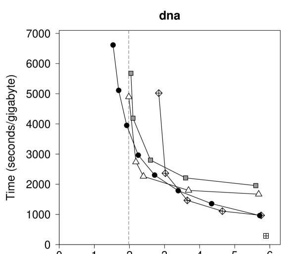
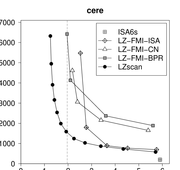
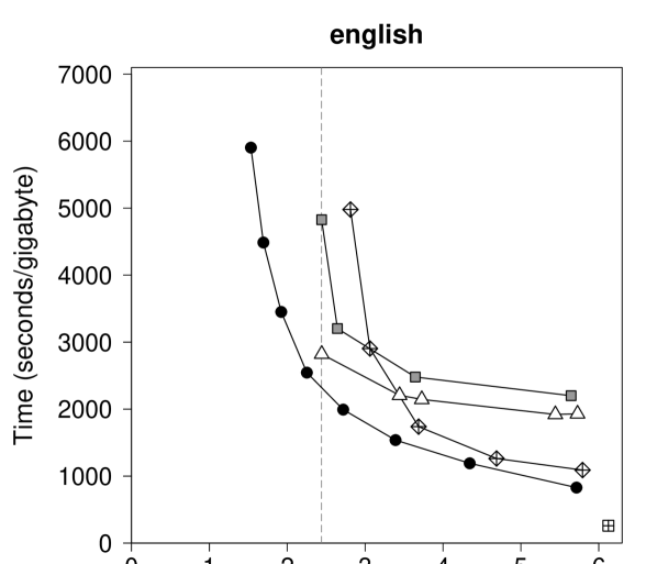
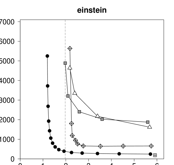
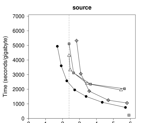
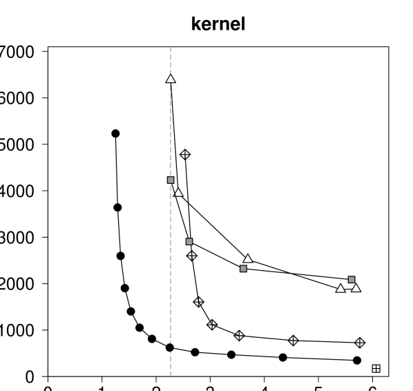
Figure 2: Time-space tradeoffs for various LZ77 factorization algorithms. The times do not include reading from or writing to disk. For algorithms with multiple parameters controlling time/space we show only the optimal points, that is, points forming the lower convex hull of the points “cloud” corresponding to various settings. The vertical line is the peak memory usage of BWT construction algorithm [25]. For comparison, we show the runtimes of $\mbox{\rm{\sf ISA}}6s$ [15], currently the fastest LZ77 factorization algorithm using $6n$ bytes.

Figure 3: Time-space tradeoffs for different variants of LZscan algorithm. The variants differ in the subprocedure computing matching statistics. Each of two approaches can be additionally boosted by enabling the “skipping trick” yielding 4 different combinations. See Section 4 for details. The times do not include reading from or writing to disk.

References

- [1] M. I. Abouelhoda, S. Kurtz, and E. Ohlebusch. Replacing suffix trees with enhanced suffix arrays. Journal of Discrete Algorithms, 2(1):53–86, 2004.
- [2] J. Barbay, T. Gagie, G. Navarro, and Y. Nekrich. Alphabet partitioning for compressed rank/select and applications. In Proc. ISAAC, LNCS 6507, pages 315–326, 2010.
- [3] M. Burrows and D. Wheeler. A block sorting lossless data compression algorithm. Technical Report 124, Digital Equipment Corporation, Palo Alto, California, 1994.
- [4] R. Cánovas and G. Navarro. Practical compressed suffix trees. In Proc. SEA, LNCS 6049, pages 94–105, 2010.
- [5] W. I. Chang and E. L. Lawler. Sublinear approximate string matching and biological applications. Algorithmica, 12(4–5):327–344, 1994.
- [6] G. Chen, S. J. Puglisi, and W. F. Smyth. Lempel-Ziv factorization using less time and space. Mathematics in Computer Science, 1(4):605–623, 2008.
- [7] M. Crochemore. String-matching on ordered alphabets. Theoretical Computer Science, 92(1):33–47, 1992.
- [8] P. Ferragina, T. Gagie, and G. Manzini. Lightweight data indexing and compression in external memory. Algorithmica, 63(3):707–730, 2012.
- [9] P. Ferragina and G. Manzini. Indexing compressed text. Journal of the ACM, 52(4):552–581, 2005.
- [10] J. Fischer and V. Heun. A new succinct representation of RMQ-information and improvements in the enhanced suffix array. In Proc. ESCAPE, LNCS 4614, pages 459–470, 2007.
- [11] T. Gagie, P. Gawrychowski, J. Kärkkäinen, Y. Nekrich, and S. J. Puglisi. A faster grammar-based self-index. In Proc. LATA, LNCS 7183, pages 240–251, 2012.
- [12] J. Kärkkäinen, D. Kempa, and S. J. Puglisi. Linear time Lempel–Ziv factorization: Simple, fast, small, 2012. Manuscript, http://arxiv.org/abs/1212.2952.
- [13] J. Kärkkäinen, G. Manzini, and S. J. Puglisi. Permuted Longest-Common-Prefix array. In Proc. CPM, LNCS 5577, pages 181–192, 2009.
- [14] T. Kasai, G. Lee, H. Arimura, S. Arikawa, and K. Park. Linear-time longest-common-prefix computation in suffix arrays and its applications. In Proc. CPM, LNCS 2089, pages 181–192, 2001.
- [15] D. Kempa and S. J. Puglisi. Lempel-Ziv factorization: fast, simple, practical. In Proc. ALENEX, pages 103–112. SIAM, 2013.
- [16] S. Kreft and G. Navarro. LZ77-like compression with fast random access. In Proc. DCC, pages 239–248, 2010.
- [17] S. Kreft and G. Navarro. Self-indexing based on LZ77. In Proc. CPM, LNCS 6661, pages 41–54, 2011.
- [18] S. Kuruppu, S. J. Puglisi, and J. Zobel. Relative Lempel-Ziv compression of genomes for large-scale storage and retrieval. In Proc. SPIRE, pages 201–206, 2010.
- [19] U. Manber and G. W. Myers. Suffix arrays: a new method for on-line string searches. SIAM Journal on Computing, 22(5):935–948, 1993.
- [20] G. Navarro. Indexing text using the Ziv-Lempel trie. Journal of Discrete Algorithms, 2(1):87–114, 2004.
- [21] G. Navarro. Indexing highly repetitive collections. In Proc. IWOCA, LNCS 7643, pages 274–279, 2012.
- [22] G. Navarro and V. Mäkinen. Compressed full-text indexes. ACM Computing Surveys, 39(1):article 2, 2007.
- [23] E. Ohlebusch and S. Gog. Lempel-Ziv factorization revisited. In Proc. CPM, LNCS 6661, pages 15–26, 2011.
- [24] D. Okanohara and K. Sadakane. An online algorithm for finding the longest previous factors. In Proc. ESA, LNCS 5193, pages 696–707, 2008.
- [25] D. Okanohara and K. Sadakane. A linear-time Burrows-Wheeler transform using induced sorting. In Proc. SPIRE, LNCS 5721, pages 696–707, 2009.
- [26] T. Starikovskaya. Computing Lempel-Ziv factorization online. In Proc. MFCS, LNCS 7464, pages 789–799, 2012.
- [27] J. Ziv and A. Lempel. A universal algorithm for sequential data compression. IEEE Transactions on Information Theory, 23(3):337–343, 1977.