A generalization of Löwner-John’s ellipsoid theorem

Abstract.

We address the following generalization $\mathbf{P}$ of the Löwner-John ellipsoid problem. Given a (non necessarily convex) compact set $\mathbf{K}\subset\mathbb{R}^{n}$ and an even integer $d\in\mathbb{N}$, find an homogeneous polynomial $g$ of degree $d$ such that $\mathbf{K}\subset\mathbf{G}:=\{\mathbf{x}:g(\mathbf{x})\leq 1\}$ and $\mathbf{G}$ has minimum volume among all such sets. We show that $\mathbf{P}$ is a convex optimization problem even if neither $\mathbf{K}$ nor $\mathbf{G}$ are convex! We next show that $\mathbf{P}$ has a unique optimal solution and a characterization with at most ${n+d-1\choose d}$ contacts points in $\mathbf{K}\cap\mathbf{G}$ is also provided. This is the analogue for $d>2$ of the Löwner-John’s theorem in the quadratic case $d=2$, but importantly, we neither require the set $\mathbf{K}$ nor the sublevel set $\mathbf{G}$ to be convex. More generally, there is also an homogeneous polynomial $g$ of even degree $d$ and a point $\mathbf{a}\in\mathbb{R}^{n}$ such that $\mathbf{K}\subset\mathbf{G}_{\mathbf{a}}:=\{\mathbf{x}:g(\mathbf{x}-\mathbf{a})\leq 1\}$ and $\mathbf{G}_{\mathbf{a}}$ has minimum volume among all such sets (but uniqueness is not guaranteed). Finally, we also outline a numerical scheme to approximate as closely as desired the optimal value and an optimal solution. It consists of solving a hierarchy of convex optimization problems with strictly convex objective function and Linear Matrix Inequality (LMI) constraints.

1. Introduction

“Approximating” data by relatively simple geometrical objects is a fundamental problem with many important applications and the ellipsoid of minimum volume is the most well-known of the associated computational techniques.

In addition to its nice properties from the viewpoint of applications, the ellipsoid of minimum volume is also very interesting from a mathematical viewpoint. Indeed, if $\mathbf{K}\subset\mathbb{R}^{n}$ is a convex body, computing an ellipsoid of minimum volume that contains $\mathbf{K}$ is a classical and famous problem which has a unique optimal solution called the Löwner-John ellipsoid. In addition, John’s theorem states that the optimal ellipsoid $\Omega$ is characterized by $s$ contacts points $\mathbf{u}_{i}\in\mathbf{K}\cap\Omega$ (more precisely $\mathbf{u}_{i}\in\partial\mathbf{K}\cap\partial\Omega$), and positive scalars $\lambda_{i}$, $i=1,\ldots,s$, where $s$ is bounded above by $n(n+3)/2$ in the general case and $s\leq n(n+1)/2$ when $\mathbf{K}$ is symmetric; see e.g. Ball [4, 5], Henk [19]. More precisely, the unit ball $B_{n}$ is the unique ellipsoid with minimum volume containing $\mathbf{K}$ if and only if $\sum_{i=1}^{s}\lambda_{i}\mathbf{u}_{i}=0$ and $\sum_{i=1}^{s}\lambda_{i}\mathbf{u}_{i}\mathbf{u}_{i}^{T}=I_{n}$, where $I_{n}$ is the $n\times n$ identity matrix.

In particular, and in contrast to other approximation techniques, computing the ellipsoid of minimum volume is a convex optimization problem for which efficient techniques are available; see e.g. Calafiore [10] and Sun and Freund [45] for more details. For a nice recent historical survey on the Löwner-John’s ellipsoid, the interested reader is referred to the recent paper by Henk [19] and the many references therein.

As underlined in Calafiore [10], “The problem of approximating observed data with simple geometric primitives is, since the time of Gauss, of fundamental importance in many scientific endeavors”. For practical purposes and numerical efficiency the most commonly used are polyhedra and ellipsoids and such techniques are ubiquitous in several different area, control, statistics, computer graphics, computer vision, to mention a few. For instance:

$\bullet$ In robust linear control, one is interested in outer or inner approximations of the stability region associated with a linear dynamical system, that is, the set of initial states from which the system can be stabilized by some control policy. Typically, the stability region which can be formulated as a semi-algebraic set in the space of coefficients of the characteristic polynomial, is non convex. By using the Hermite stability criterion, it can be described by a parametrized polynomial matrix inequality where the parameters account for uncertainties and the variables are the controller coefficients. Convex inner approximations of the stability region have been proposed in form of polytopes in Nurges [35], ellipsoids in Henrion et al. [22], and more general convex sets defined by Linear Matrix Inequalities (LMIs) in Henrion et al. [24], and Karimi et al. [27].

$\bullet$ In statistics one is interested in the ellipsoid $\xi$ of minimum volume covering some given $k$ of $m$ data points because $\xi$ has some interesting statistical properties such as affine equivariance and positive breakdown properties [12]. In this context the center of the ellipsoid is called the minimum volume ellipsoid (MVE) location estimator and the associated matrix associated with $\xi$ is called the MVE scatter estimator; see e.g. Rousseeuw [43] and Croux et al. [12].

$\bullet$ In pattern separation, minimum volume ellipsoids are used for separating two sets of data points. For computing such ellipsoids, convex programming techniques have been used in the early work of Rosen [40] and more modern semidefinite programming techniques in Vandenberghe and Boyd [47]. Similarly, in robust statistics and data mining the ellipsoid of minimum volume covering a finite set of data points identifies outliers as the points on its boundary; see e.g. Rousseeuw and Leroy [43]. Moreover, this ellipsoid technique is also scale invariant, a highly desirable property in data mining which is not enjoyed by other clustering methods based on various distances; see the discussion in Calafiore [10], Sun and Freund [45] and references therein.

$\bullet$ Other clustering techniques in computer graphics, computer vision and pattern recognition, use various (geometric or algebraic) distances (e.g. the equation error) and compute the best ellipsoid by minimizing an associated non linear least squares criterion (whence the name “least squares fitting ellipsoid” methods). For instance, such techniques have been proposed in computer graphics and computer vision by Bookstein [9] and Pratt [37], in pattern recognition by Rosin [41], Rosin and West [42], Taubin [46], and in another context by Chernousko [11]. When using an algebraic distance (like e.g. the equation error) the geometric interpretation is not clear and the resulting ellipsoid may not be satisfactory; see e.g. an illuminating discussion in Gander et al. [17]. Moreover, in general the resulting optimization problem is not convex and convergence to a global minimizer is not guaranteed.

So optimal data fitting using an ellipsoid of minimum volume is not only satisfactory from the viewpoint of applications but is also satisfactory from a mathematical viewpoint as it reduces to a (often tractable) convex optimization problem with a unique solution having a nice characterization in term of contact points in $\mathbf{K}\cap\Omega$. In fact, reduction to solving a convex optimization problem with a unique optimal solution, is a highly desirable property of any data fitting technique!

A more general optimal data fitting problem

In the Löwner-John problem one restricts to convex bodies $\mathbf{K}$ because for a non convex set $\mathbf{K}$ the optimal ellipsoid is also solution to the problem where $\mathbf{K}$ is replaced with its convex hull ${\rm co}(\mathbf{K})$. However, if one considers sets that are more general than ellipsoids, an optimal solution for $\mathbf{K}$ is not necessarily the same as for ${\rm co}(\mathbf{K})$, and indeed, in some applications one is interested in approximating as closely as desired a non convex set $\mathbf{K}$. In this case a non convex approximation is sometimes highly desirable as more efficient.

For instance, in the robust control problem already alluded to above, in Henrion and Lasserre [23] we have provided an inner approximation of the stability region $\mathbf{K}$ by the sublevel set $\mathbf{G}=\{\mathbf{x}:g(\mathbf{x})\leq 0\}$ of a non convex polynomial $g$. By allowing the degree of $g$ to increase one obtains the convergence ${\rm vol}(\mathbf{G})\to{\rm vol}(\mathbf{K})$ which is impossible with convex polytopes, ellipsoids and LMI approximations as described in [35, 22, 24, 27].

So if one considers the more general data fitting problem where $\mathbf{K}$ and/or the (outer) approximating set are allowed to be non convex, can we still infer interesting conclusions as for the Löwner-John problem? Can we also derive a practical algorithm for computing (or at least approximating) an optimal solution?

The purpose of this paper is to provide results in this direction that can be seen as a non convex generalization of the Lowner-John problem but, surprisingly, still reduces to solving a convex optimization problem with a unique optimal solution.

Some works have considered generalizations of the Löwner-John problem. Fo instance, Giannopoulos et al. [13] have extended John’s theorem for couples $(\mathbf{K}_{1},\mathbf{K}_{2})$ of convex bodies when $\mathbf{K}_{1}$ is in maximal volume position of $\mathbf{K}_{1}$ inside $\mathbf{K}_{2}$, whereas Bastero and Romance [7] refined this result by allowing $\mathbf{K}_{1}$ to be non-convex.

In this paper we consider a different non convex generalization of the Löwner-John ellipsoid problem, with a more algebraic flavor. Namely, we address the following two problems $\mathbf{P}_{0}$ and $\mathbf{P}$.

$\mathbf{P}_{0}$: Let $\mathbf{K}\subset\mathbb{R}^{n}$ be a compact set (not necessarily convex) and let $d$ be an even integer. Find an homogeneous polynomial $g$ of degree $d$ such that its sublevel set $\mathbf{G}_{1}:=\{\mathbf{x}\,:\,g(\mathbf{x})\leq 1\}$ contains $\mathbf{K}$ and has minimum volume among all such sublevel sets with this inclusion property.

$\mathbf{P}$: Let $\mathbf{K}\subset\mathbb{R}^{n}$ be a compact set (not necessarily convex) and let $d$ be an even integer. Find an homogeneous polynomial $g$ of degree $d$ and $\mathbf{a}\in\mathbb{R}^{n}$ such that the sublevel set $\mathbf{G}_{1}^{\mathbf{a}}:=\{\mathbf{x}\,:\,g(\mathbf{x}-\mathbf{a})\leq 1\}$ contains $\mathbf{K}$ and has minimum volume among all such sublevel sets with this inclusion property.

Necessarily $g$ is a nonnegative homogeneous polynomial since otherwise the volumes of $\mathbf{G}_{1}$ and $\mathbf{G}^{\mathbf{a}}_{1}$ are not finite. Of course, when $d=2$ then $g$ is convex (i.e., $\mathbf{G}_{1}$ and $\mathbf{G}^{\mathbf{a}}_{1}$ are ellipsoids) because every nonnegative quadratic form defines a convex function, and $g$ is an optimal solution for problem $\mathbf{P}$ with $\mathbf{K}$ or its convex hull ${\rm co}(\mathbf{K})$. That is, one retrieves the Löwner-John problem. But when $d>2$ then $\mathbf{G}_{1}$ and $\mathbf{G}_{1}^{\mathbf{a}}$ are not necessarily convex. For instance, take $\mathbf{K}=\{\mathbf{x}:g(\mathbf{x})\leq 1\}$ where $g$ is some nonnegative homogeneous polynomial such that $\mathbf{K}$ is compact but non convex. Then $g$ is an optimal solution for problem $\mathbf{P}_{0}$ with $\mathbf{K}$ and cannot be optimal for ${\rm co}(\mathbf{K})$; a two-dimensional example is $(x,y)\mapsto g(x,y):=x^{4}+y^{4}-\epsilon x^{2}y^{2}$ and another one is $g(x,y):=x^{6}+y^{6}-\epsilon x^{3}y^{3}$, for $\epsilon>0$ sufficiently small; see Figure 1.

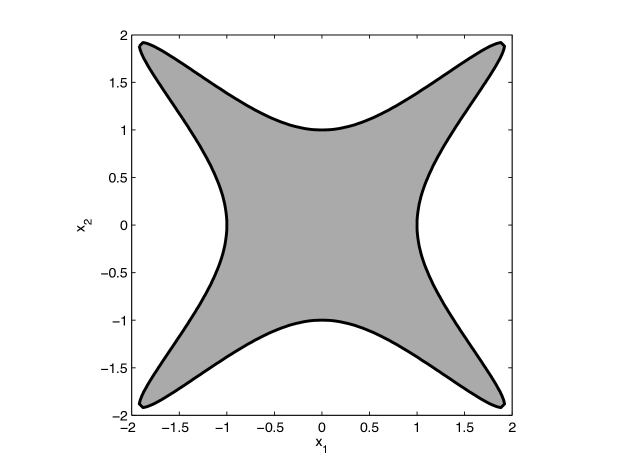
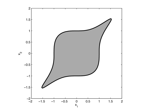
Figure 1. $\mathbf{G}_{1}$ with $g(\mathbf{x})=x^{4}+y^{4}-1.925\,x^{2}y^{2}$ (left) and with $g(\mathbf{x})=x^{6}+y^{6}-1.925\,x^{3}y^{3}$ (right)

Contribution

We show that problem $\mathbf{P}_{0}$ and $\mathbf{P}$ are indeed natural generalizations of the Löwner-John ellipsoid problem in the sense that:

- (a) $\mathbf{P}_{0}$ also has a unique solution $g^{*}$.

- (b) A characterization of $g^{*}$ also involves $s$ contact points in $\mathbf{K}\cap\mathbf{G}_{1}$ (more precisely in $\partial\mathbf{K}\cap\partial\mathbf{G}_{1}$), where $s$ is now bounded by ${n+d-1\choose d}$ (when $d=2$ one retrieves the bound for the symmetric Löwner-John problem).

And so when $d=2$ we retrieve the symmetric Löwner-John problem as a particular case. In fact it is shown that $\mathbf{P}_{0}$ is a convex optimization problem no matter if neither $\mathbf{K}$ nor $\mathbf{G}_{1}$ are convex. Of course, convexity in itself does not guarantee a favorable computational complexity. As we will see $\mathbf{P}_{0}$ reduces to minimizing a strictly convex function over a convex cone intersected with an affine subspace and “hardness” of $\mathbf{P}_{0}$ is reflected in two of its components: (i) The (convex) objective function as well as its gradient and Hessian are difficult to evaluate, and (ii) the cone membership problem is NP-hard in general. However convexity is crucial to show the uniqueness and characterization of the optimal solution in (a) and (b) above.

We use an intermediate and crucial result of independent interest. Namely, the Lebesgue-volume function $g\mapsto v(g):={\rm vol}(\mathbf{G}_{1})$ is a strictly convex function of the coefficients of $g$, which is far from being obvious from its definition. Concerning the more general problem $\mathbf{P}$, we also show that there is an optimal solution $(g^{*},\mathbf{a}^{*})$ with again a characterization which involves $s$ contact points in $\mathbf{K}\cap\mathbf{G}^{\mathbf{a}^{*}}_{1}$, but now uniqueness is not guaranteed. Again and importantly, in both problems $\mathbf{P}_{0}$ and $\mathbf{P}$, neither $\mathbf{K}$ nor $\mathbf{G}_{1}^{\mathbf{a}}$ are required to be convex.

On the computational side

Even though $\mathbf{P}_{0}$ is a convex optimization problem, it is hard to solve because even if $\mathbf{K}$ would be a finite set of points (as is the case in statistics applications of the Löwner-John problem) and in contrast to the quadratic case, evaluating the (strictly convex) objective function, its gradient and Hessian can be a challenging problem, especially if the dimension is larger than $n=3$. Indeed evaluating the objective function reduces to computing the Lebesgue volume of the sublevel set $\mathbf{G}_{1}$ whereas evaluating its gradient and Hessian requires computing other moments of the Lebesgue measure on $\mathbf{G}_{1}$. So this is one price to pay for the generalization of the Löwner-John ellipsoid problem. (Notice however that if $\mathbf{K}$ is not a finite set of points then even the Löwner-John ellipsoid problem is also hard to solve because for more general sets $\mathbf{K}$ the inclusion constraint $\mathbf{K}\subset\xi$ (or ${\rm conv}(\mathbf{K})\subset\xi$) can be difficult to handle.) In general, and even for convex bodies, computing the volume is an NP-hard problem; in fact even approximating the volume efficiently within given bounds is hopeless. For more details the interested reader is referred to e.g. Barvinok [6], Dyer et al. [14] and the many references therein. On the other hand, even though $\mathbf{G}_{1}$ is not necessarily convex, it is still a rather specific set and assessing a precise computational complexity for its volume remains to be done.

However, we can still approximate as closely as desired the objective function as well as its gradient and Hessian by using the methodology developed in Henrion et al [21], especially when the dimension is small $n=2,3$ (which is the case in several applications in statistics).

Moreover, if $\mathbf{K}$ is a (compact) basic semi-algebraic set with an explicit description $\{\mathbf{x}:g_{j}(\mathbf{x})\geq 0,\>j=1,\ldots,m\}$ for some polynomials $(g_{j})\subset\mathbb{R}[\mathbf{x}]$, then we can use powerful positivity certificates from real algebraic geometry to handle the inclusion constraint $\mathbf{G}_{1}\supset\mathbf{K}$ in the associated convex optimization problem. Therefore, in this context, we also provide a numerical scheme to approximate the optimal value and the unique optimal solution of $\mathbf{P}_{0}$ as closely as desired. It consists of solving a hierarchy of convex optimization problems where each problem in the hierarchy has a strictly convex objective function and a feasible set defined by Linear Matrix Inequalities (LMIs).

2. Notation, definitions and preliminary results

2.1. Notation and definitions

Let $\mathbb{R}[\mathbf{x}]$ be the ring of polynomials in the variables $\mathbf{x}=(x_{1},\ldots,x_{n})$ and let $\mathbb{R}[\mathbf{x}]_{d}$ be the vector space of polynomials of degree at most $d$ (whose dimension is $s(d):={n+d\choose n}$). For every $d\in\mathbb{N}$, let $\mathbb{N}^{n}_{d}:=\{\alpha\in\mathbb{N}^{n}:|\alpha|\,(=\sum_{i}\alpha_{i})\leq d\}$, and let $\mathbf{v}_{d}(\mathbf{x})=(\mathbf{x}^{\alpha})$, $\alpha\in\mathbb{N}^{n}$, be the vector of monomials of the canonical basis $(\mathbf{x}^{\alpha})$ of $\mathbb{R}[\mathbf{x}]_{d}$. For two real symmetric matrices $\mathbf{B},\mathbf{C}$, the notation $\langle\mathbf{B},\mathbf{C}\rangle$ stands for ${\rm trace}\,(\mathbf{B}\mathbf{C})$; also, the notation $\mathbf{B}\succeq 0$ (resp. $\mathbf{B}\succ 0$) stands for $\mathbf{B}$ is positive semidefinite (resp. positive definite). A polynomial $f\in\mathbb{R}[\mathbf{x}]_{d}$ is written

$$\mathbf{x}\mapsto f(\mathbf{x})\,=\,\sum_{\alpha\in\mathbb{N}^{n}}f_{\alpha}\,\mathbf{x}^{\alpha},$$

for some vector of coefficients $\mathbf{f}=(f_{\alpha})\in\mathbb{R}^{s(d)}$. A polynomial $f\in\mathbb{R}[\mathbf{x}]_{d}$ is homogeneous of degree $d$ if $f(\lambda\mathbf{x})=\lambda^{d}f(\mathbf{x})$ for all $\mathbf{x}\in\mathbb{R}^{n}$ and all $\lambda\in\mathbb{R}$.

Let us denote by $\mathbf{H}[\mathbf{x}]_{d}$, $d\in\mathbb{N}$, the space of homogeneous polynomials of degree $d$ and $\mathbf{P}[\mathbf{x}]_{d}\subset\mathbf{H}[\mathbf{x}]_{d}$, its subset of homogeneous polynomials of degree $d$ such that their sublevel set $\mathbf{G}_{1}:=\{\,\mathbf{x}\,:\,g(\mathbf{x})\leq 1\,\}$ has finite Lebesgue volume, denoted ${\rm vol}(\mathbf{G}_{1})$. Notice that $g\in\mathbf{P}[\mathbf{x}]_{d}$ is necessarily nonnegative (so that $d$ is necessarily even) and $0\not\in\mathbf{P}[\mathbf{x}]_{d}$; but $\mathbf{P}[\mathbf{x}]_{d}$ is not the set of positive semidefinite (psd) forms of degree $d$ (excluding the zero form); indeed if $n=2$ and $\mathbf{x}\mapsto g(\mathbf{x})=(x_{1}-x_{2})^{2}$ then $\mathbf{G}_{1}$ does not have finite Lebesgue volume. On the other hand when $g\in\mathbf{P}[\mathbf{x}]_{d}$ the set $\mathbf{G}_{1}$ is not necessarily bounded; for instance if $n=2$ and $\mathbf{x}\mapsto g(\mathbf{x}):=x_{1}^{2}x_{2}^{2}(x_{1}^{2}+x_{2}^{2})$, the set $\mathbf{G}_{1}$ has finite volume but is not bounded. So $\mathbf{P}[\mathbf{x}]_{d}$ is not the space of positive definite (pd) forms of degree $d$ either.

For $d\in\mathbb{N}$ and a closed set $\mathbf{K}\subset\mathbb{R}^{n}$, denote by $C_{d}(\mathbf{K})$ the convex cone of all polynomials of degree at most $d$ that are nonnegative on $\mathbf{K}$, and denote by $\mathcal{M}(\mathbf{K})$ the Banach space of finite signed Borel measures with support contained in $\mathbf{K}$ (equipped with the total variation norm). Let $\mathcal{M}(\mathbf{K})_{+}\subset\mathcal{M}(\mathbf{K})$ be the convex cone of finite (positive) Borel measures on $\mathbf{K}$.

In the Euclidean space $\mathbb{R}^{n}$ we denote by $\langle\cdot,\cdot\rangle$ the usual duality bracket.

Laplace transform

Given a measurable function $f:\mathbb{R}\to\mathbb{R}$ with $f(t)=0$ for all $t<0$, its one-sided (or unilateral) Laplace transform $\mathcal{L}[f]:\mathbb{C}\to\mathbb{C}$ is defined by

$$\lambda\mapsto\quad\mathcal{L}[f](\lambda)\,:=\,\int_{0}^{\infty}\exp(-\lambda t)f(t)\,dt,\qquad\lambda\in\,D,$$

where its domain $D\subset\mathbb{C}$ is the set of $\lambda\in\mathbb{C}$ where the above integral is finite. For instance, let $f(t)=0$ if $t<0$ and $f(t)=t^{a}$ for $t\geq 0$ and $a>-1$. Then $\mathcal{L}[f](\lambda)=\frac{\Gamma(a+1)}{\lambda^{a+1}}$ and $D=\{\lambda:\Re(\lambda)>0\}$. Moreover $\mathcal{L}[f]$ is analytic on $D$ and therefore if there exists an analytic function $F$ such that $\mathcal{L}[f](\lambda)=F(\lambda)$ for all $\lambda$ in a segment of the real line contained in $D$, then $\mathcal{L}[f](\lambda)=F(\lambda)$ for all $\lambda\in D$. This is a consequence of the Identity Theorem for analytic functions; see e.g. Freitag and Busam [16, Theorem III.3.2, p. 125]. A classical reference for the Laplace transform is Widder [48].

2.2. Some preliminary results

We first have the following result:

Lemma 2.1.

The set $\mathbf{P}[\mathbf{x}]_{d}$ is a convex cone.

Proof.

Let $g,h\in\mathbf{P}[\mathbf{x}]_{d}$ with associated sublevel sets $\mathbf{G}_{1}=\{\mathbf{x}:g(\mathbf{x})\leq 1\}$ and $\mathbf{H}_{1}=\{\mathbf{x}:h(\mathbf{x})\leq 1\}$. For $\lambda\in(0,1)$, consider the nonnegative homogeneous polynomial $\theta:=\lambda g+(1-\lambda)h\in\mathbb{R}[\mathbf{x}]_{d}$, with associated sublevel set

$$\Theta_{1}\,:=\,\{\mathbf{x}\>:\>\theta(\mathbf{x})\,\leq\,1\}\,=\,\{\mathbf{x}\>:\>\lambda g(\mathbf{x})+(1-\lambda)h(\mathbf{x})\,\leq\,1\}.$$

Write $\Theta_{1}=\Theta_{1}^{1}\cup\Theta_{1}^{2}$ where $\Theta_{1}^{1}=\Theta_{1}\cap\{\mathbf{x}:g(\mathbf{x})\geq h(\mathbf{x})\}$ and $\Theta_{1}^{2}=\Theta_{1}\cap\{\mathbf{x}:g(\mathbf{x})<h(\mathbf{x})\}$. Observe that $\mathbf{x}\in\Theta_{1}^{1}$ implies $h(\mathbf{x})\leq 1$ and so $\Theta_{1}^{1}\subset\mathbf{H}_{1}$. Similarly $\mathbf{x}\in\Theta_{1}^{2}$ implies $g(\mathbf{x})\leq 1$ and so $\Theta_{1}^{2}\subset\mathbf{G}_{1}$. Therefore ${\rm vol}(\Theta_{1})\leq{\rm vol}(\mathbf{G}_{1})+{\rm vol}(\mathbf{H}_{1})<\infty$. And so $\theta\in\mathbf{P}[\mathbf{x}]_{d}$. ∎

With $y\in\mathbb{R}$ and $g\in\mathbb{R}[\mathbf{x}]$ let $\mathbf{G}_{y}:=\{\mathbf{x}:g(\mathbf{x})\leq y\}$. The following intermediate result which is crucial and of independent interest was already proved in Morozov and Shakirov [33, 34] with different arguments.

Theorem 2.2.

Let $g\in\mathbf{P}[\mathbf{x}]_{d}$. Then for every $y\geq 0$:

(2.1) $${\rm vol}(\mathbf{G}_{y})\,=\,\frac{y^{n/d}}{\Gamma(1+n/d)}\,\int_{\mathbb{R}^{n}}\exp(-g(\mathbf{x}))\,d\mathbf{x}.$$

Proof.

As $g\in\mathbf{P}[\mathbf{x}]_{d}$, and using homogeneity, ${\rm vol}(\mathbf{G}_{1})<\infty$ implies ${\rm vol}(\mathbf{G}_{y})<\infty$ for every $y\geq 0$. Let $h:\mathbb{R}\to\mathbb{R}$ be the function $y\mapsto h(y):={\rm vol}(\mathbf{G}_{y})$. Since $g$ is nonnegative, the function $h$ vanishes on $(-\infty,0]$. Its Laplace transform $\mathcal{L}[h]:\mathbb{C}\to\mathbb{C}$ is the function

$$\lambda\mapsto\mathcal{L}[h](\lambda):=\int_{0}^{\infty}\exp(-\lambda y)h(y)\,dy,\qquad\Re(\lambda)\,>\,0,$$

whose domain is $D=\{\lambda\in\mathbb{C}:\>\Re(\lambda)>0\}$. Observe that whenever $\lambda\in\mathbb{R}$ with $\lambda>0$,

$$\mathcal{L}[h](\lambda) = \int_{0}^{\infty}\exp(-\lambda y)\left(\displaystyle\int_{\{\mathbf{x}:g(\mathbf{x})\leq y\}}d\mathbf{x}\right)\,dy$$

$$= \displaystyle\int_{\mathbb{R}^{n}}\left(\int_{g(\mathbf{x})}^{\infty}\exp(-\lambda y)dy\right)\,d\mathbf{x}\quad\mbox{[by Fubini's Theorem]}$$

$$= \frac{1}{\lambda}\displaystyle\int_{\mathbb{R}^{n}}\,\exp(-\lambda g(\mathbf{x}))\,d\mathbf{x}$$

$$= \frac{1}{\lambda}\displaystyle\int_{\mathbb{R}^{n}}\,\exp(-g(\lambda^{1/d}\mathbf{x}))\,d\mathbf{x}\quad\mbox{[by homogeneity]}$$

$$= \frac{1}{\lambda^{1+n/d}}\displaystyle\int_{\mathbb{R}^{n}}\exp(-g(\mathbf{z}))\,d\mathbf{z}\quad\mbox{[by $\lambda^{1/d}\mathbf{x}\to\mathbf{z}$]}$$

$$= \underbrace{\frac{\displaystyle\int_{\mathbb{R}^{n}}\exp(-g(\mathbf{z}))\,d\mathbf{z}}{\Gamma(1+n/d)}}_{{\rm constant}\,c}\>\frac{\Gamma(1+n/d)}{\lambda^{1+n/d}}.$$

Next, the function $\lambda\mapsto\frac{c\,\Gamma(1+n/d)}{\lambda^{1+n/d}}$ is analytic on $D$ and coincide with $\mathcal{L}[h]$ on the real half-line $\{t:t>0\}$ contained in $D$. Therefore by the Identity Theorem $\mathcal{L}[h](\lambda)=\frac{c\,\Gamma(1+n/d)}{\lambda^{1+n/d}}$ on $D$. Finally observe that $\frac{\Gamma(1+n/d)}{\lambda^{1+n/d}}$ is the Laplace transform of $t\mapsto u(t)=t^{n/d}$, which yields the desired result $h(y)={\rm vol}(\mathbf{G}_{y})=c\,y^{n/d}$. ∎

And we also conclude:

Corollary 2.3.

Let $g\in\mathbf{H}[\mathbf{x}]_{d}$. Then $g\in\mathbf{P}[\mathbf{x}]_{d}$, i.e. ${\rm vol}(\mathbf{G}_{1})<\infty$, if and only if $\displaystyle\int_{\mathbb{R}^{n}}\exp(-g(\mathbf{x}))d\mathbf{x}<\infty$.

Proof.

The implication $\Rightarrow$ follows from Theorem 2.2. For the reverse implication consider the function $u:\mathbb{R}^{n}\times\mathbb{R}_{+}\to\mathbb{R}$ defined by $(\mathbf{x},y)\mapsto u(\mathbf{x},y):=\exp(-y)\,I_{\{\mathbf{x}:g(\mathbf{x})\leq y\}}$, which is measurable and nonnegative. Therefore by Tonelli’s Theorem (see e.g. Royden [44]):

$$\int_{\mathbb{R}^{n}}\int_{\mathbb{R}_{+}}u(\mathbf{x},y)\,d\mathbf{x}\,dy = \int_{\mathbb{R}^{n}}\left(\underbrace{\int_{\mathbb{R}_{+}}u(\mathbf{x},y)\,dy}_{\exp(-g(\mathbf{x}))}\right)\,d\mathbf{x}\,<\,\infty$$

$$= \int_{\mathbb{R}_{+}}\left(\int_{\mathbb{R}^{n}}u(\mathbf{x},y)\,d\mathbf{x}\,\right)\,dy$$

$$= \int_{\mathbb{R}_{+}}\exp(-y)\,\left(\underbrace{\int_{\mathbb{R}^{n}}I_{\{\mathbf{x}:g(\mathbf{x})\leq y\}}\,d\mathbf{x}}_{{\rm vol}\,(\mathbf{G}_{y})}\right)\,dy.$$

Therefore ${\rm vol}\,(\mathbf{G}_{y})$ is finite (and so is $\mathbf{G}_{1}$). ∎

As already mentioned, Formula (2.1) relating the Lebesgue volume $\mathbf{G}_{1}$ with the integral $\int\exp(-g)$ is already proved (with a different argument) in Morozov and Shakirov [33, 34] where the authors want to express the non Gaussian integral $\int\exp(-g)$ in terms of algebraic invariants of $g$.

Sensitivity analysis and convexity

We now investigate some properties of the function $v:\mathbf{P}[\mathbf{x}]_{d}\to\mathbb{R}$ defined by

(2.2) $$g\,\mapsto\,v(g)\,:=\,{\rm vol}(\mathbf{G}_{1})\,=\,\int_{\{\mathbf{x}\>:\>g(\mathbf{x})\leq 1\}}d\mathbf{x},\qquad g\in\mathbf{P}(\mathbf{x}]_{d},$$

i.e., we now view ${\rm vol}(\mathbf{G}_{1})$ as a function of the vector $\mathbf{g}=(g_{\alpha})\in\mathbb{R}^{\ell(d)}$ of coefficients of $g$ in the canonical basis of homogeneous polynomials of degree $d$ (and $\ell(d)={n+d-1\choose d}$).

Theorem 2.4.

The Lebesgue-volume function $v:\mathbf{P}(\mathbf{x}]_{d}\to\mathbb{R}$ defined in (2.2) is strictly convex and lower semi-continuous. In ${\rm int}(\mathbf{P}[\mathbf{x}]_{d})$ its gradient $\nabla v$ and Hessian $\nabla^{2}v$ are given by:

(2.3) $$\frac{\partial v(g)}{\partial g_{\alpha}}\,=\,\frac{-1}{\Gamma(1+n/d)}\int_{\mathbb{R}^{n}}\mathbf{x}^{\alpha}\,\exp(-g(\mathbf{x}))\,d\mathbf{x},$$

for all $\alpha\in\mathbb{N}^{n}_{d}$, $|\alpha|=d$.

(2.4) $$\frac{\partial^{2}v(g)}{\partial g_{\alpha}\partial g_{\beta}}\,=\,\frac{1}{\Gamma(1+n/d)}\int_{\mathbb{R}^{n}}\mathbf{x}^{\alpha+\beta}\,\exp(-g(\mathbf{x}))\,d\mathbf{x},$$

for all $\alpha,\beta\,\in\mathbb{N}^{n}_{d}$, $|\alpha|=|\beta|=d$. Moreover, we also have

(2.5) $$\int_{\mathbb{R}^{n}}g(\mathbf{x})\,\exp(-g(\mathbf{x}))\,d\mathbf{x}\,=\,\frac{n}{d}\,\int_{\mathbb{R}^{n}}\exp(-g(\mathbf{x}))\,d\mathbf{x}.$$

Proof.

By Theorem 2.2 $v(g)=c\int_{\mathbb{R}^{n}}\exp(-g(\mathbf{x}))d\mathbf{x}$ with $c=\Gamma(1+n/d)^{-1}$. Let $p,q\in\mathbf{P}[\mathbf{x}]_{d}$ and $\alpha\in[0,1]$. By convexity of $u\mapsto\exp(-u)$,

$$v(\alpha p+(1-\alpha)q) \leq c\,\displaystyle\int_{\mathbb{R}^{n}}[\,\alpha\exp(-p(\mathbf{x}))+(1-\alpha)\exp(-q(\mathbf{x}))\,]\,d\mathbf{x}$$

$$= \alpha v(p)+(1-\alpha)v(q),$$

and so $v$ is convex. Next, in view of the strict convexity of $u\mapsto\exp(-u)$, equality may occur only if $p(\mathbf{x})=q(\mathbf{x})$ almost everywhere, which implies $p=q$ and which in turn implies strict convexity of $v$. To get the lower-semicontinuity, let $(g_{n})\subset\mathbf{P}[\mathbf{x}]_{d}$ be such that $g_{n}\to g$ as $n\to\infty$ and $\liminf_{h\to g}v(h)=\lim_{n\to\infty}v(g_{n})$. Then $g_{n}(\mathbf{x})\to g(\mathbf{x})$ pointwise and by Fatou lemma (since $v\geq 0$)

$$\liminf_{h\to g}v(h)\,=\,\liminf_{n\to\infty}\int_{\mathbb{R}^{n}}\exp(-g_{n})\,d\mathbf{x} \geq \int_{\mathbb{R}^{n}}\liminf_{n\to\infty}\exp(-g_{n})\,d\mathbf{x}$$

$$= \int_{\mathbb{R}^{n}}\exp(-g)\,d\mathbf{x}\,=\,v(g).$$

To obtain (2.3)-(2.4) when $g\in{\rm int}(\mathbf{P}[\mathbf{x}]_{d})$, one takes partial derivatives under the integral sign, which in this context is allowed. Indeed, write $g$ in the canonical basis as $g(\mathbf{x})=\sum_{|\alpha|=d}g_{\alpha}\mathbf{x}^{\alpha}$. For every $\alpha\in\mathbb{N}^{n}_{d}$ with $|\alpha|=d$, let $(e_{\alpha})\subset\mathbb{R}^{\ell(d)}$ be the standard unit vectors of $\mathbb{R}^{\ell(d)}$. Then for every $t>0$ sufficiently small, $\mathbf{x}\mapsto g(\mathbf{x})+t\mathbf{x}^{\alpha}\in\mathbf{P}[\mathbf{x}]_{d}$ and

$$\frac{v(g+te_{\alpha})-v(g)}{t}\,=\,c\,\int_{\mathbb{R}^{n}}\exp(-g)\,\left(\underbrace{\frac{\exp(-t\mathbf{x}^{\alpha})-1}{t}}_{\psi(t,\mathbf{x})}\right)\,d\mathbf{x}<\infty$$

Notice that for every $\mathbf{x}$, by convexity of the function $t\mapsto\exp(-t\mathbf{x}^{\alpha})$,

$$\lim_{t\downarrow 0}\psi(t,\mathbf{x})\,=\,\inf_{t>0}\psi(t,\mathbf{x})\,=\,\exp(-t\mathbf{x}^{\alpha})^{\prime}_{|t=0}\,=\,-\mathbf{x}^{\alpha},$$

because for every $\mathbf{x}$, the function $t\mapsto\psi(t,\mathbf{x})$ is nondecreasing; see e.g. Rockafellar [39, Theorem 23.1]. Hence, the one-sided directional derivative $v^{\prime}(g;e_{\alpha})$ in the direction $e_{\alpha}$ satisfies

$$v^{\prime}(g;e_{\alpha}) = \lim_{t\downarrow 0}\frac{v(g+te_{\alpha})-v(g)}{t}\,=\,\lim_{t\downarrow 0}\,c\,\int_{\mathbb{R}^{n}}\exp(-g)\,\psi(t,\mathbf{x})\,d\mathbf{x}$$

$$= c\,\int_{\mathbb{R}^{n}}\exp(-g)\,\lim_{t\downarrow 0}\psi(t,\mathbf{x})\,d\mu(\mathbf{x})\,=\,c\,\int_{\mathbb{R}^{n}}-\mathbf{x}^{\alpha}\exp(-g)\,d\mathbf{x},$$

where the third equality follows from the Extended Monotone Convergence Theorem [3, 1.6.7]. Indeed for all $t<t_{0}$ with $t_{0}$ sufficiently small, the function $\psi(t,\cdot)$ is bounded above by $\psi(t_{0},\cdot)$ and $\int_{\mathbb{R}^{n}}\exp(-g)\psi(t_{0},\mathbf{x})d\mu<\infty$. Similarly, for every $t>0$

$$\frac{v(g-te_{\alpha})-v(g)}{t}\,=\,c\,\int_{\mathbb{R}^{n}}\exp(-g)\,\underbrace{\frac{\exp(t\mathbf{x}^{\alpha})-1}{t}}_{\xi(t,\mathbf{x})}\,d\mathbf{x},$$

and by convexity of the function $t\mapsto\exp(t\mathbf{x}^{\alpha})$

$$\lim_{t\downarrow 0}\xi(t,\mathbf{x})\,=\,\inf_{t>0}\xi(t,\mathbf{x})\,=\,\exp(t\mathbf{x}^{\alpha})^{\prime}_{|t=0}\,=\,\mathbf{x}^{\alpha}.$$

Therefore, with exactly same arguments as before,

$$v^{\prime}(g;-e_{\alpha}) = \lim_{t\downarrow 0}\frac{v(g-te_{\alpha})-v(g)}{t}$$

$$= c\,\int_{\mathbb{R}^{n}}\mathbf{x}^{\alpha}\exp(-g)\,d\mathbf{x}=-v^{\prime}(g;e_{\alpha}),$$

and so

$$\frac{\partial v(g)}{\partial g_{\alpha}}\,=\,-c\,\int_{\mathbb{R}^{n}}\mathbf{x}^{\alpha}\,\exp(-g)\,d\mathbf{x},$$

for every $\alpha$ with $|\alpha|=d$, which yields (2.3). Similar arguments can used for the Hessian $\nabla^{2}v(g)$ which yields (2.4).

To obtain (2.5) observe that $g\mapsto H(g):=\int\exp(-g)d\mathbf{x}$, $g\in\mathbf{P}[\mathbf{x}]_{d}$, is a positively homogeneous function of degree $-n/d$, continuously differentiable. And so combining (2.3) with Euler’s identity $\langle\nabla H(g),g\rangle=-nH(g)/d$, yields:

$$-\frac{n}{d}\int_{\mathbb{R}^{n}}\exp(-g(\mathbf{x}))\,d\mathbf{x} = -\frac{n}{d}\,H(g)$$

$$= \langle\nabla H(g),g\rangle\quad\mbox{[by Euler's identity]}$$

$$= -\int_{\mathbb{R}^{n}}g(\mathbf{x})\,\exp(-g(\mathbf{x}))\,d\mathbf{x}.$$

∎

Notice that convexity of $v$ is not obvious at all from its definition (2.2) whereas it becomes almost transparent when using formula (2.1).

2.3. The dual cone of $C_{d}(\mathbf{K})$

For a convex cone $C\subset\mathbb{R}^{n}$, the convex cone

$$C^{*}\,:=\,\{\,\mathbf{y}\>:\>\langle\mathbf{y},\mathbf{x}\rangle\,\geq\,0\quad\forall\,\mathbf{x}\,\in\,C\,\},$$

is called the dual cone of $C$, and if $C$ is closed then $(C^{*})^{*}=C$. Recall that for a set $\mathbf{K}\subset\mathbb{R}^{n}$, $C_{d}(\mathbf{K})$ denotes the convex cone of polynomials of degree at most $d$ which are nonnegative on $\mathbf{K}$. We say that a vector $\mathbf{y}\in\mathbb{R}^{s(d)}$ has a representing measure (or is a $d$-truncated moment sequence) if there exists a finite Borel measure $\phi$ on $\mathbb{R}^{n}$ such that

$$y_{\alpha}\,=\,\int_{\mathbb{R}^{n}}\mathbf{x}^{\alpha}\,d\phi,\qquad\forall\alpha\in\mathbb{N}^{n}_{d}.$$

We will need the following (already known) characterization the dual cone $C_{d}(\mathbf{K})^{*}$ (which is also transparent in [18, §1.1, p. 852]).

Lemma 2.5.

Let $\mathbf{K}\subset\mathbb{R}^{n}$ be compact. For every $d\in\mathbb{N}$, the dual cone $C_{d}(\mathbf{K})^{*}$ is the convex cone

(2.6) $$\Delta_{d}\,:=\,\left\{\left(\int_{\mathbf{K}}\mathbf{x}^{\alpha}\,d\phi\right),\>\alpha\in\mathbb{N}^{n}_{d}\>:\>\phi\in\mathcal{M}(\mathbf{K})_{+}\>\right\},$$

i.e., the convex cone of vectors of $\mathbb{R}^{s(d)}$ which have a representing measure with support contained in $\mathbf{K}$.

Proof.

For every $\mathbf{y}=(y_{\alpha})\in\Delta_{d}$ and $f\in C_{d}(\mathbf{K})$ with coefficient vector $\mathbf{f}\in\mathbb{R}^{s(d)}$:

(2.7) $$\langle\mathbf{y},\mathbf{f}\rangle\,=\,\sum_{\alpha\in\mathbb{N}^{n}_{d}}f_{\alpha}\,y_{\alpha}\,=\,\sum_{\alpha\in\mathbb{N}^{n}_{d}}\int_{\mathbf{K}}f_{\alpha}\,\mathbf{x}^{\alpha}\,d\phi\,=\,\int_{\mathbf{K}}f\,d\phi\,\geq\,0.$$

Since (2.7) holds for all $f\in C_{d}(\mathbf{K})$ and all $\mathbf{y}\in\Delta_{d}$, then necessarily $\Delta_{d}\subseteq C_{d}(\mathbf{K})^{*}$ and similarly, $C_{d}(\mathbf{K})\subseteq\Delta_{d}^{*}$. Next,

$$\Delta_{d}^{*} = \left\{\mathbf{f}\in\mathbb{R}^{s(d)}\>:\>\langle\mathbf{f},\mathbf{y}\rangle\geq 0\quad\forall\mathbf{y}\in\Delta_{d}\right\}$$

$$= \left\{f\in\mathbb{R}[\mathbf{x}]_{d}\>:\>\int_{\mathbf{K}}f\,d\phi\geq 0\quad\forall\phi\in\mathcal{M}(\mathbf{K})_{+}\right\}$$

$$\Rightarrow \Delta_{d}^{*}\subseteq C_{d}(\mathbf{K}),$$

and so $\Delta_{d}^{*}=C_{d}(\mathbf{K})$. Hence the result follows if one proves that $\Delta_{d}$ is closed, because then $C_{d}(\mathbf{K})^{*}=(\Delta_{d}^{*})^{*}=\Delta_{d}$, the desired result. So let $(\mathbf{y}^{k})\subset\Delta_{d}$, $k\in\mathbb{N}$, with $\mathbf{y}^{k}\to\mathbf{y}$ as $k\to\infty$. Equivalently, $\int_{\mathbf{K}}\mathbf{x}^{\alpha}d\phi_{k}\to y_{\alpha}$ for all $\alpha\in\mathbb{N}^{n}_{d}$. In particular, the convergence $y^{k}_{0}\to y_{0}$ implies that the sequence of measures $(\phi_{k})$, $k\in\mathbb{N}$, is bounded, that is, $\sup_{k}\phi_{k}(\mathbf{K})<M$ for some $M>0$. As $\mathbf{K}$ is compact, the unit ball of $\mathcal{M}(\mathbf{K})$ is sequentially compact in the weak $\star$ topology $\sigma(\mathcal{M}(\mathbf{K}),C(\mathbf{K}))$ where $C(\mathbf{K})$ is the space of continuous functions on $\mathbf{K}$. Hence there is a finite Borel measure $\phi\in\mathcal{M}(\mathbf{K})_{+}$ and a subsequence $(k_{i})$ such that $\int_{\mathbf{K}}gd\phi_{k_{i}}\to\int_{\mathbf{K}}gd\phi$ as $i\to\infty$, for all $g\in C(\mathbf{K})$. In particular, for every $\alpha\in\mathbb{N}^{n}_{d}$,

$$y_{\alpha}\,=\,\lim_{k\to\infty}y^{k}_{\alpha}\,=\,\lim_{i\to\infty}y^{k_{i}}_{\alpha}\,=\,\lim_{i\to\infty}\int_{\mathbf{K}}\mathbf{x}^{\alpha}d\phi_{k_{i}}\,=\,\int_{\mathbf{K}}\mathbf{x}^{\alpha}d\phi,$$

which shows that $\mathbf{y}\in\Delta_{d}$, and so $\Delta_{d}$ is closed. ∎

And we also have:

Lemma 2.6.

Let $\mathbf{K}\subset\mathbb{R}^{n}$ be with nonempty interior. Then the interior of $C_{d}(\mathbf{K})^{*}$ is nonempty.

Proof.

Since $C_{d}(\mathbf{K})$ is nonempty and closed, by Faraut and Korány [15, Prop. I.1.4, p. 3]

$${\rm int}(C_{d}(\mathbf{K})^{*})\,=\,\{\,\mathbf{y}\>:\>\langle\mathbf{y},\mathbf{g}\rangle>0,\quad\forall g\in C_{d}(\mathbf{K})\setminus\{0\}\,\},$$

where $\mathbf{g}\in\mathbb{R}^{s(d)}$ is the coefficient of $g\in C_{d}(\mathbf{K})$, and

$${\rm int}(C_{d}(\mathbf{K})^{*})\,\neq\,\emptyset\Longleftrightarrow C_{d}(\mathbf{K})\cap(-C_{d}(\mathbf{K}))\,=\,\{0\}.$$

But $g\in C_{d}(\mathbf{K})\cap(-C_{d}(\mathbf{K}))$ implies $g\geq 0$ and $g\leq 0$ on $\mathbf{K}$, which in turn implies $g=0$ because $\mathbf{K}$ has nonempty interior. ∎

For simplicity and with a slight abuse of notation, we will sometimes write $\langle\mathbf{z},g\rangle$ in lieu of $\langle\mathbf{z},\mathbf{g}\rangle$ and $\langle\mathbf{z},1-g\rangle$ in lieu of $\langle\mathbf{z},e_{0}-\mathbf{g}\rangle$ (where $e_{0}$ is the unit vector corresponding to the constant polynomial equal to 1).

3. Main result

Consider the following problem $\mathbf{P}_{0}$, a non convex generalization of the Löwner-John ellipsoid problem:

$\mathbf{P}_{0}$: Let $\mathbf{K}\subset\mathbb{R}^{n}$ be a compact set not necessarily convex and $d$ an even integer. Find an homogeneous polynomial $g$ of degree $d$ such that its sublevel set $\mathbf{G}_{1}:=\{\mathbf{x}\,:\,g(\mathbf{x})\leq 1\}$ contains $\mathbf{K}$ and has minimum volume among all such sublevel sets with this inclusion property.

In the above problem $\mathbf{P}_{0}$, the set $\mathbf{G}_{1}$ is symmetric and so when $\mathbf{K}$ is a symmetric convex body and $d=2$, one retrieves the Löwner-John ellipsoid problem in the symmetric case. In the next section we will consider the more general case where $\mathbf{G}_{1}$ is of the form $\mathbf{G}_{1}^{\mathbf{a}}:=\{\mathbf{x}:g(\mathbf{x}-\mathbf{a})\leq 1\}$ for some $\mathbf{a}\in\mathbb{R}^{n}$ and some $g\in\mathbf{P}[\mathbf{x}]_{d}$.

Recall that $\mathbf{P}[\mathbf{x}]_{d}\subset\mathbb{R}[\mathbf{x}]_{d}$ is the convex cone of nonnegative homogeneous polynomials of degree $d$ whose sublevel set $\mathbf{G}_{1}=\{\mathbf{x}:g(\mathbf{x})\leq 1\}$ has finite volume. Recall also that $C_{d}(\mathbf{K})\subset\mathbb{R}[\mathbf{x}]_{d}$ is the convex cone of polynomials of degree at most $d$ that are nonnegative on $\mathbf{K}$.

We next show that solving $\mathbf{P}_{0}$ is equivalent to solving the convex optimization problem:

(3.1) $$\mathcal{P}:\qquad\rho=\displaystyle\inf_{g\in\mathbf{H}[\mathbf{x}]_{d}}\>\left\{\,\int_{\mathbb{R}^{n}}\exp(-g)\,d\mathbf{x}\>:\>1-g\,\in\,C_{d}(\mathbf{K})\,\right\}.$$

Proposition 3.1.

Problem $\mathbf{P}_{0}$ has an optimal solution if and only if problem $\mathcal{P}$ in (3.1) has an optimal solution. Moreover, $\mathcal{P}$ is a finite-dimensional convex optimization problem.

Proof.

By Theorem 2.2,

$${\rm vol}\,(\mathbf{G}_{1})\,=\,\frac{1}{\Gamma(1+n/d)}\int_{\mathbb{R}^{n}}\exp(-g)\,d\mathbf{x}$$

whenever $\mathbf{G}_{1}$ has finite Lebesgue volume. Moreover $\mathbf{G}_{1}$ contains $\mathbf{K}$ if and only if $1-g\in C_{d}(\mathbf{K})$ and so $\mathbf{P}_{0}$ has an optimal solution $g^{*}\in\mathbf{P}[\mathbf{x}]_{d}$ if and only if $g^{*}$ is an optimal solution of $\mathcal{P}$ (with value ${\rm vol}(\mathbf{G}^{*}_{1})\Gamma(1+n/d)$). Now since $g\mapsto\int_{\mathbb{R}^{n}}\exp(-g)d\mathbf{x}$ is strictly convex (by Lemma 2.4) and both $C_{d}(\mathbf{K})$ and $\mathbf{P}[\mathbf{x}]_{d}$ are convex cones, problem $\mathcal{P}$ is a finite-dimensional convex optimization problem. ∎

We now can state the first main result of this paper: Recall that $\mathcal{M}(\mathbf{K})_{+}$ is the convex cone of finite Borel measures on $\mathbf{K}$.

Theorem 3.2.

Let $\mathbf{K}\subset\mathbb{R}^{n}$ be compact with nonempty interior and consider the convex optimization problem $\mathcal{P}$ in (3.1).

(a) $\mathcal{P}$ has a unique optimal solution $g^{*}\in\mathbf{P}[\mathbf{x}]_{d}$.

(b) Let $g^{*}\in\mathbf{P}[\mathbf{x}]_{d}$ be the unique optimal solution of $\mathcal{P}$ and let $\mathbf{G}^{*}_{1}=\{\,\mathbf{x}:g^{*}(\mathbf{x})\leq 1\,\}$. If $g^{*}\in{\rm int}(\mathbf{P}[\mathbf{x}]_{d})$ then there exists a finite Borel measure $\mu^{*}\in\mathcal{M}(\mathbf{K})_{+}$ such that

(3.2) $$\int_{\mathbb{R}^{n}}\mathbf{x}^{\alpha}\exp(-g^{*})d\mathbf{x} = \int_{\mathbf{K}}\mathbf{x}^{\alpha}\,d\mu^{*},\qquad\forall|\alpha|=d$$

(3.3) $$\int_{\mathbf{K}}(1-g^{*})\,d\mu^{*} = 0;\quad\mu^{*}(\mathbf{K})=\frac{n}{d}\int_{\mathbb{R}^{n}}\exp(-g^{*})\,d\mathbf{x}.$$

In particular, $\mu^{*}$ is supported on the set $V:=\{\mathbf{x}\in\mathbf{K}:g^{*}(\mathbf{x})=1\}\,(=\mathbf{K}\cap\mathbf{G}^{*}_{1})$ and in fact, $\mu^{*}$ can be substituted with another measure $\nu^{*}\in\mathcal{M}(\mathbf{K})_{+}$ supported on at most ${n+d-1\choose d}$ contact points of $V$.

(c) Conversely, if $g^{*}\in\mathbb{R}[\mathbf{x}]_{d}$ is homogeneous with $1-g^{*}\in C_{d}(\mathbf{K})$, and there exist points $(\mathbf{x}_{i},\lambda_{i})\in\mathbf{K}\times\mathbb{R}$, $\lambda_{i}>0$, $i=1,\ldots,s$, such that $g^{*}(\mathbf{x}_{i})=1$ for all $i=1,\ldots,s$, and

$$\int_{\mathbb{R}^{n}}\mathbf{x}^{\alpha}\exp(-g^{*})\,d\mathbf{x}\,=\,\sum_{i=1}^{s}\lambda_{i}\,\mathbf{x}_{i}^{\alpha},\qquad|\alpha|=d,$$

then $g^{*}$ is the unique optimal solution of problem $\mathcal{P}$.

The proof is postponed to §7. Importantly, notice that neither $\mathbf{K}$ nor $\mathbf{G}^{*}_{1}$ are required to be convex. If the optimal solution $g^{*}\not\in{\rm int}(\mathbf{P}[\mathbf{x}]_{d})$ then $\mu^{*}$ satisfies an analogue of (3.2) which now involves a subgradient $\partial v(g^{*})$ at $g^{*}$ of the function $g\mapsto v(g)=\int\exp(-g)d\mathbf{x}$. That is, $(\int_{\mathbf{K}}\mathbf{x}^{\alpha}d\mu^{*})_{|\alpha|=d}\in-\partial v(g^{*})$.

3.1. On the contact points

Theorem 3.2 states that $\mathcal{P}$ (hence $\mathbf{P}_{0}$) has a unique optimal solution $g^{*}\in\mathbf{P}[\mathbf{x}]_{d}$ and if $g^{*}\in{\rm int}(\mathbf{P}[\mathbf{x}]_{d})$ one may find contact points $\mathbf{x}_{i}\in\mathbf{K}\cap\mathbf{G}^{*}_{1}$, $i=1,\ldots,s$, with $s\leq{n+d-1\choose d}$, such that

(3.4) $$y^{*}_{\alpha}\,=\,\int_{\mathbb{R}^{n}}\mathbf{x}^{\alpha}\,\exp(-g^{*}(\mathbf{x}))\,d\mathbf{x}\,=\,\sum_{i=1}^{s}\lambda_{i}\,\mathbf{x}_{i}^{\alpha},\quad|\alpha|=d,$$

for some positive weights $\lambda_{i}$. In particular, using the identity (2.5) and $\langle 1-g^{*},\mathbf{y}^{*}\rangle=0$, as well as $g^{*}(\mathbf{x}_{i})=1$ for all $i$,

$$y^{*}_{0}\,=\,\sum_{|\alpha|=d}y^{*}_{\alpha}\,g^{*}_{\alpha}\,=\,\frac{n}{d}\int_{\mathbb{R}^{n}}\exp(-g^{*}(\mathbf{x}))\,d\mathbf{x}\,=\,\sum_{i=1}^{s}\lambda_{i}.$$

Next, recall that $d$ is even and let $\mathbf{v}_{d/2}:\mathbb{R}^{n}\to\mathbb{R}^{\ell(d/2)}$ be the mapping

$$\mathbf{x}\mapsto\mathbf{v}_{d/2}(\mathbf{x})=(\mathbf{x}^{\alpha}),\qquad|\alpha|\,=\,d/2,$$

i.e., the ${n-1+d/2\choose d/2}$-vector of the canonical basis of $\mathbf{H}[\mathbf{x}]_{d/2}$. From (3.4),

(3.5) $$\int_{\mathbb{R}^{n}}\mathbf{v}_{d/2}(\mathbf{x})\,\mathbf{v}_{d/2}(\mathbf{x})^{T}\exp(-g^{*})\,d\mathbf{x}\,=\,\sum_{i=1}^{s}\lambda_{i}\,\mathbf{v}_{d/2}(\mathbf{x}_{i})\,\mathbf{v}_{d/2}(\mathbf{x}_{i})^{T}.$$

Hence, when $d=2$ and $\mathbf{K}$ is symmetric, one retrieves the characterization in John’s theorem [19, Theorem 2.1], namely that if the euclidean ball $\xi_{n}:=\{\mathbf{x}:\|\mathbf{x}\|\leq 1\}$ is the unique ellipsoid of minimum volume containing $\mathbf{K}$ then there are contact points $(\mathbf{x}_{i})\subset\xi_{n}\cap\mathbf{K}$ and positive weights $(\lambda_{i})$, such that $\sum_{i}\lambda_{i}\mathbf{x}_{i}\mathbf{x}_{i}^{T}=I_{n}$ (where $I_{n}$ is the $n\times n$ identity matrix). Indeed in this case, $\mathbf{v}_{d/2}(\mathbf{x})=\mathbf{x}$, $g^{*}(\mathbf{x})=\|\mathbf{x}\|^{2}$ and $\int_{\mathbb{R}^{n}}\mathbf{x}\mathbf{x}^{T}\exp(-\|\mathbf{x}\|^{2})d\mathbf{x}=c\,I_{n}$ for some constant $c$.

So (3.5) is the analogue for $d>2$ of the contact-points property in John’s theorem and we obtain the following generalization: For $d$ even, let $\|\mathbf{x}\|_{d}:=(\sum_{i=1}^{n}x_{i}^{d})^{1/d}$ denote the $d$-norm with unit ball $\xi^{d}_{n}:=\{\mathbf{x}:\|\mathbf{x}\|_{d}\leq 1\}$.

Corollary 3.3.

If in Theorem 3.2 the unique optimal solution $\mathbf{G}^{*}_{1}$ is the $d$-unit ball $\xi^{d}_{n}$ then there are contact points $(\mathbf{x}_{i})\subset\mathbf{K}\cap\xi^{d}_{n}$ and positive weights $\lambda_{i}$, $i=1,\ldots,s$, with $s\leq{n+d-1\choose d}$, such that for every $|\alpha|=d$,

$$\sum_{i=1}^{s}\lambda_{i}\,\mathbf{v}_{d/2}(\mathbf{x}_{i})\mathbf{v}_{d/2}(\mathbf{x}_{i})^{T}\,=\,\int_{\mathbb{R}^{n}}\mathbf{v}_{d/2}(\mathbf{x})\mathbf{v}_{d/2}(\mathbf{x})^{T}\exp(-\|\mathbf{x}\|^{d}_{d})\,d\mathbf{x}.$$

Equivalently, for $|\alpha|=d$,

$$\sum_{i=1}^{s}\lambda_{i}\,\mathbf{x}_{i}^{\alpha}\,=\,\left\{\begin{array}[]{ll}\displaystyle\prod_{j=1}^{n}\displaystyle\int_{\mathbb{R}}t^{\alpha_{j}}\exp(-t^{d})\,dt&\mbox{if $\alpha=2\beta$}\\ 0&\mbox{otherwise.}\end{array}\right.$$

Example

With $n=2$ let $\mathbf{K}\subset\mathbb{R}^{2}$ be the box $[-1,1]^{2}$ and let $d=4,6$, that is, one searches for the unique homogeneous polynomial $g\in\mathbb{R}[\mathbf{x}]_{4}$ or $g\in\mathbb{R}[\mathbf{x}]_{6}$ which contains $\mathbf{K}$ and has minimum volume among such sets.

Theorem 3.4.

The sublevel set $\mathbf{G}^{4}_{1}=\{\,\mathbf{x}:g_{4}(\mathbf{x})\leq 1\,\}$ associated with the homogeneous polynomial

(3.6) $$\mathbf{x}\mapsto g_{4}(\mathbf{x})\,=\,x_{1}^{4}+x_{2}^{4}-x_{1}^{2}x_{2}^{2},$$

is the unique solution of problem $\mathbf{P}_{0}$ with $d=4$. That is, $\mathbf{K}\subset\mathbf{G}_{1}^{4}$ and $\mathbf{G}^{4}_{1}$ has minimum volume among all sets $\mathbf{G}_{1}\supset\mathbf{K}$ defined with homogeneous polynomials of degree $4$.

Similarly, the sublevel set $\mathbf{G}^{6}_{1}=\{\,\mathbf{x}:g_{6}(\mathbf{x})\leq 1\,\}$ associated with the homogeneous polynomial

(3.7) $$\mathbf{x}\mapsto g_{6}(\mathbf{x})\,=\,x_{1}^{6}+x_{2}^{6}-(x_{1}^{4}x_{2}^{2}+x_{1}^{2}x_{2}^{4})/2$$

is the unique solution of problem $\mathbf{P}_{0}$ with $d=6$.

Proof.

Let $g_{4}$ be as in (3.6) (hence in ${\rm int}(\mathbf{P}[\mathbf{x}]_{d})$). We first prove that $\mathbf{K}\subset\mathbf{G}_{1}^{4}$, i.e., $1-g_{4}(\mathbf{x})\geq 0$ whenever $\mathbf{x}\in\mathbf{K}$. But observe that if $\mathbf{x}\in\mathbf{K}$ then

$$1-g_{4}(\mathbf{x}) = 1-x_{1}^{4}-x_{2}^{4}+x_{1}^{2}x_{2}^{2}\,=\,1-x_{1}^{4}+x_{2}^{2}(x_{1}^{2}-x_{2}^{2})$$

$$\geq 1-x_{1}^{4}+x_{2}^{2}(x_{1}^{2}-1)\quad\mbox{[as $-x_{2}^{2}\geq-1$ and $x_{2}^{2}\geq 0$]}$$

$$\geq (1-x_{1}^{2})\,(1+x_{1}^{2}-x_{2}^{2})$$

$$\geq (1-x_{1}^{2})\,x_{1}^{2}\,\geq\,0\quad\mbox{[as $-x_{2}^{2}\geq-1$ and $1-x_{1}^{2}\geq 0$]}.$$

Hence $1-g_{4}\in C_{d}(\mathbf{K})$. Observe that $\mathbf{K}\cap\mathbf{G}_{1}^{4}$ consists of the $8$ contact points $(\pm 1,\pm 1)$ and $(0,\pm 1)$, $(\pm 1,0)$. Next let $\nu^{*}$ be the measure defined by

(3.8) $$\nu^{*}\,=\,a\,(\delta_{(-1,1)}+\delta_{(1,1)})+b\,(\delta_{(1,0)}+\delta_{(0,1)})$$

where $\delta_{\mathbf{x}}$ denote the Dirac measure at $\mathbf{x}$ and $a,b\geq 0$ are chosen to satisfy

$$2\,a\,+\,b\,=\,\int_{\mathbb{R}^{n}}x_{1}^{4}\,\exp(-g_{4})\,d\mathbf{x};\quad 2\,a\,=\,\int_{\mathbb{R}^{n}}x_{1}^{2}x_{2}^{2}\,\exp(-g_{4})\,d\mathbf{x},$$

so that

$$\int\mathbf{x}^{\alpha}\,d\nu^{*}\,=\,\int_{\mathbb{R}^{n}}\mathbf{x}^{\alpha}\,\exp(-g_{4}(\mathbf{x}))\,d\mathbf{x},\quad|\alpha|=4.$$

Of course a unique solution $(a,b)\geq 0$ exists since

$$\int_{\mathbb{R}^{n}}x_{1}^{4}\,\exp(-g_{4})\,d\mathbf{x}\int_{\mathbb{R}^{n}}x_{2}^{4}\,\exp(-g_{4})\,d\mathbf{x} = \left(\int_{\mathbb{R}^{n}}x_{1}^{4}\,\exp(-g_{4})\,d\mathbf{x}\right)^{2}$$

$$\geq \left(\int_{\mathbb{R}^{n}}x_{1}^{2}x_{2}^{2}\,\exp(-g_{4})\,d\mathbf{x}\right)^{2}.$$

Therefore the measure $\nu^{*}$ is indeed as in Theorem 3.2(c) and the proof is completed. Notice that as predicted by Theorem 3.2(b), $\nu^{*}$ is supported on $4\leq{n+d-1\choose d}=5$ points. Similarly with $g_{6}$ as in (3.7) and $\mathbf{x}\in\mathbf{K}$,

$$1-g_{6}(\mathbf{x}) = 1-x_{1}^{6}-x_{2}^{6}+(x_{1}^{4}x_{2}^{2}+x_{1}^{2}x_{2}^{4})/2$$

$$= (1-x_{1}^{6})/2+(1-x_{2}^{6})/2-x_{1}^{4}(x_{1}^{2}-x_{2}^{2})/2-x_{2}^{4}(x_{2}^{2}-x_{1}^{2})/2$$

$$\geq (1-x_{1}^{6})/2+(1-x_{2}^{6})/2-x_{1}^{4}(1-x_{2}^{2})/2-x_{2}^{4}(1-x_{1}^{2})/2$$

[as $$-x_{1}^{6}\geq-x_{1}^{4} -x_{2}^{6}\geq-x_{2}^{4}$$ and ]

$$\geq (1-x_{1}^{2})(1+x_{1}^{2}+x_{1}^{4}-x_{2}^{4})/2+(1-x_{2}^{2})(1+x_{2}^{2}+x_{2}^{4}-x_{1}^{4})/2$$

$$\geq (1-x_{1}^{2})(x_{1}^{2}+x_{1}^{4})/2+(1-x_{2}^{2})(x_{2}^{2}+x_{2}^{4})/2\,\geq 0$$

$$\mbox{[as $1-x_{1}^{4}\geq 0$ and $1-x_{2}^{4}\geq 0$]}.$$

So again the measure $\nu^{*}$ defined in (3.8) where $a,b\geq 0$ are chosen to satisfy

$$2\,a\,+\,b\,=\,\int_{\mathbb{R}^{n}}x_{1}^{6}\,\exp(-g_{6})\,d\mathbf{x};\quad 2\,a\,=\,\int_{\mathbb{R}^{n}}x_{1}^{4}x_{2}^{2}\,\exp(-g_{6})\,d\mathbf{x},$$

is such that

$$\int\mathbf{x}^{\alpha}\,d\mu^{*}\,=\,\int_{\mathbb{R}^{n}}\mathbf{x}^{\alpha}\,\exp(-g_{6}(\mathbf{x}))\,d\mathbf{x},\quad|\alpha|=6.$$

Again a unique solution $(a,b)\geq 0$ exists because

$$\left(\int_{\mathbb{R}^{n}}x_{1}^{6}\,\exp(-g_{6})\,d\mathbf{x}\right)\left(\int_{\mathbb{R}^{n}}x_{1}^{2}x_{2}^{4}\,\exp(-g_{6})\,d\mathbf{x}\right)\,\geq\,\left(\int_{\mathbb{R}^{n}}x_{1}^{4}x_{2}^{2}\,\exp(-g_{6})\,d\mathbf{x}\right)^{2}.$$

∎

With $d=4$, the non convex sublevel set $\mathbf{G}_{1}^{4}=\{\mathbf{x}:g_{4}(\mathbf{x})\leq 1\}$ which is displayed in Figure 2 (left) is a much better approximation of $\mathbf{K}=[-1,1]^{2}$ than the ellipsoid of minimum volume $\xi=\{\mathbf{x}:\|\mathbf{x}\|^{2}\leq 2\}$ that contains $\mathbf{K}$. In particular, ${\rm vol}(\xi)=2\pi\approx 6.28$ whereas ${\rm vol}(\mathbf{G}_{1}^{4})\approx 4.32$.

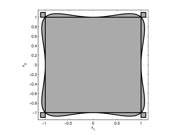
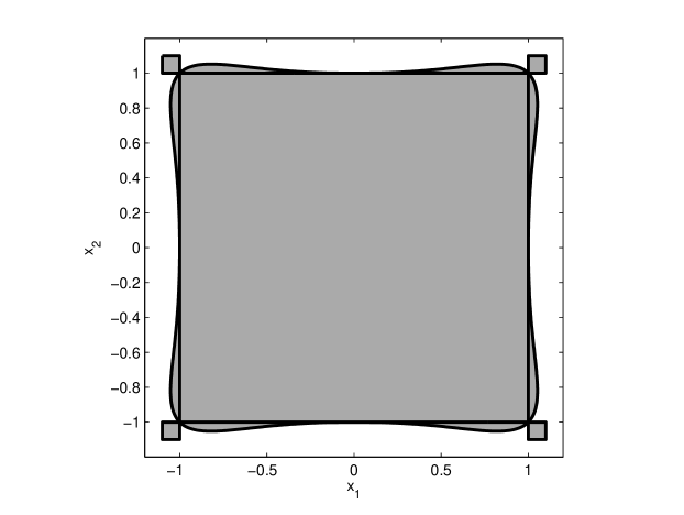
Figure 2. $\mathbf{K}=[-1,1]^{2}$ and $\mathbf{G}_{1}^{4}=\{\mathbf{x}:x_{1}^{4}+x_{2}^{4}-x_{1}^{2}x_{2}^{2}\leq 1\}$ (left), $\mathbf{G}_{1}^{6}=\{\mathbf{x}:x_{1}^{6}+x_{2}^{6}-(x_{1}^{4}x_{2}^{2}+x_{1}^{2}x_{2}^{4})/2\leq 1\}$ (right)

With $d=6$, the non convex sublevel set $\mathbf{G}_{1}^{6}=\{\mathbf{x}:g_{6}(\mathbf{x})\leq 1\}$ which is displayed in Figure 2 (right) is again a better approximation of $\mathbf{K}=[-1,1]^{2}$ than the ellipsoid of minimum volume $\xi=\{\mathbf{x}:\|\mathbf{x}\|^{2}\leq 2\}$ that contains $\mathbf{K}$, and as ${\rm vol}(\mathbf{G}_{1}^{6})\approx 4.1979$ it provides a better approximation than the sublevel set $\mathbf{G}_{1}^{4}$ with $d=4$.

Finally if $\mathbf{K}=\mathbf{G}_{1}^{6}$ then $\mathbf{G}_{1}^{4}$ is an optimal solution of $\mathbf{P}_{0}$ with $d=4$, that is $\mathbf{G}_{1}^{4}$ has minimum volume among all sets $\mathbf{G}_{1}\supset\mathbf{G}_{1}^{6}$ defined by homogeneous polynomials $g\in\mathbf{P}[\mathbf{x}]_{4}$. Indeed first we have solved the polynomial optimization problem: $\rho=\inf_{\mathbf{x}}\{1-g_{4}(\mathbf{x}):1-g_{6}(\mathbf{x})\geq 0\}$ via the hierarchy of semidefinite relaxations defined in [30, 31] and at the fifth semidefinite relaxation (i.e. with moments of order $12$) we found $\rho=0$ with the eight contact points $(\pm 1,\pm 1),(\pm 1,0),(0,\pm 1)\in\mathbf{G}_{1}^{4}\cap\mathbf{G}_{1}^{6}$ as global minimizers! This shows (up to $10^{-9}$ numerical precision) that $\mathbf{G}_{1}^{6}\subset\mathbf{G}_{1}^{4}$. Then again the measure $\nu^{*}$ defined in (3.8) satisfies Theorem 3.2(b) and so $g_{4}$ is an optimal solution of problem $\mathbf{P}_{0}$ with $\mathbf{K}=\mathbf{G}_{1}^{6}$ and $d=4$.

At last, the ball $\mathbf{G}_{1}^{2}=\{\mathbf{x}:(x_{1}^{2}+x_{2}^{2})/2\leq 1\}$ is an optimal solution of $\mathbf{P}_{0}$ with $d=2$ and we have $\mathbf{K}\subset\mathbf{G}_{1}^{6}\subset\mathbf{G}_{1}^{4}\subset\mathbf{G}_{1}^{2}$.

4. The general case

We now consider the more general case where the set $\mathbf{G}_{1}$ is of the form $\{\mathbf{x}:g(\mathbf{x}-\mathbf{a})\leq 1\}=:\mathbf{G}_{1}^{\mathbf{a}}$ where $\mathbf{a}\in\mathbb{R}^{n}$ and $g\in\mathbf{P}[\mathbf{x}]_{d}$.

For every $\mathbf{a}\in\mathbb{R}^{n}$ and $g\in\mathbb{R}[\mathbf{x}]_{d}$ (with coefficient vector $\mathbf{g}\in\mathbb{R}^{s(d)}$) define the polynomial $g_{\mathbf{a}}\in\mathbb{R}[\mathbf{x}]_{d}$ by $\mathbf{x}\mapsto g_{\mathbf{a}}(\mathbf{x}):=g(\mathbf{x}-\mathbf{a})$ and its sublevel set $\mathbf{G}_{1}^{\mathbf{a}}:=\{\mathbf{x}:g_{\mathbf{a}}(\mathbf{x})\leq 1\}$. The polynomial $g_{\mathbf{a}}$ can be written

(4.1) $$g_{\mathbf{a}}(\mathbf{x})\,=\,g(\mathbf{x}-\mathbf{a})\,=\,\sum_{\alpha\in\mathbb{N}^{n}_{d}}p_{\alpha}(\mathbf{a},\mathbf{g})\,\mathbf{x}^{\alpha},$$

where $\mathbf{g}\in\mathbb{R}^{s(d)}$ and the polynomial $p_{\alpha}\in\mathbb{R}[\mathbf{x},\mathbf{g}]$ is linear in $\mathbf{g}$, for every $\alpha\in\mathbb{N}^{n}_{d}$. Consider the following generalization of $\mathbf{P}_{0}$:

$\mathbf{P}$: Let $\mathbf{K}\subset\mathbb{R}^{n}$ be a compact set not necessarily convex and $d\in\mathbb{N}$ an even integer. Find an homogeneous polynomial $g$ of degree $d$ and a point $\mathbf{a}\in\mathbb{R}^{n}$ such that the sublevel set $\mathbf{G}_{1}^{\mathbf{a}}:=\{\mathbf{x}\,:\,g(\mathbf{x}-\mathbf{a})\leq 1\}$ contains $\mathbf{K}$ and has minimum volume among all such sublevel sets with this inclusion property.

When $d=2$ one retrieves the general (non symmetric) Löwner-John ellipsoid problem. For $d>2$, an even more general problem would be to find a (non homogeneous) polynomial $g$ of degree $d$ such that $\mathbf{K}\subset\mathbf{G}_{1}=\{\mathbf{x}:g(\mathbf{x})\leq 1\}$ and $\mathbf{G}_{1}$ has minimum volume among all such set $\mathbf{G}_{1}$ with this inclusion property. However when $g$ is not homogeneous we do not have an analogue of Theorem 2.2 for the Lebesgue-volume ${\rm vol}(\mathbf{G}_{1})$.

So in view of (4.3), one wishes to solve the optimization problem

(4.2) $$\mathcal{P}:\quad\rho=\min_{\mathbf{a}\in\mathbb{R}^{n},g\in\mathbf{P}[\mathbf{x}]_{d}}\>\{{\rm vol}(\mathbf{G}^{\mathbf{a}}_{1})\>:\>1-g_{\mathbf{a}}\in C_{d}(\mathbf{K})\},$$

a generalization of (3.1) where $\mathbf{a}=0$. In contrast to $\mathbf{P}_{0}$, problem $\mathbf{P}$ is not convex and so computing a global optimal solution is more difficult. In particular we do not provide an analogue of the numerical scheme for $\mathbf{P}_{0}$ described in §5 and the results of this section are mostly of theoretical interest. However we still can show that for every optimal solution $(\mathbf{a}^{*},g^{*})\in\mathbb{R}^{n}\times\mathbf{P}[\mathbf{x}]_{d}$, there is a characterization of $\mathbf{G}_{1}^{\mathbf{a}^{*}}$ similar to the one obtained for $\mathbf{P}_{0}$.

Let $\mathbf{K}-\mathbf{a}$ denotes the set $\{\mathbf{x}-\mathbf{a}:\mathbf{x}\in\mathbf{K}\}$, and observe that whenever $g\in\mathbf{P}[\mathbf{x}]_{d}$,

(4.3) $${\rm vol}(\mathbf{G}_{1}^{\mathbf{a}})\,=\,{\rm vol}(\mathbf{G}_{1}^{0})\,=\,{\rm vol}(\mathbf{G}_{1})\,=\,\frac{1}{\Gamma(1+n/d)}\int_{\mathbb{R}^{n}}\exp(-g(\mathbf{x}))\,d\mathbf{x}.$$

Theorem 4.1.

Let $\mathbf{K}\subset\mathbb{R}^{n}$ be compact with nonempty interior and consider the optimization problem $\mathcal{P}$ in (4.2).

(a) $\mathcal{P}$ has an optimal solution $(\mathbf{a}^{*},g^{*})\in\mathbb{R}^{n}\times\mathbf{P}[\mathbf{x}]_{d}$.

(b) Let $(\mathbf{a}^{*},g^{*})\in\mathbb{R}^{n}\times\mathbf{P}[\mathbf{x}]_{d}$ be an optimal solution of $\mathcal{P}$. If $g^{*}\in{\rm int}(\mathbf{P}[\mathbf{x}]_{d})$ then there exists a finite Borel measure $\mu^{*}\in\mathcal{M}(\mathbf{K}-\mathbf{a}^{*})_{+}$ such that

(4.4) $$\int_{\mathbb{R}^{n}}\mathbf{x}^{\alpha}\exp(-g^{*})d\mathbf{x} = \int_{\mathbf{K}-\mathbf{a}^{*}}\mathbf{x}^{\alpha}\,d\mu^{*},\qquad\forall|\alpha|=d$$

(4.5) $$\int_{\mathbf{K}-\mathbf{a}^{*}}(1-g^{*})\,d\mu^{*} = 0;\quad\mu^{*}(\mathbf{K}-\mathbf{a}^{*})=\frac{n}{d}\int_{\mathbb{R}^{n}}\exp(-g^{*})\,d\mathbf{x}.$$

In particular, $\mu^{*}$ is supported on the set $V:=\{\mathbf{x}\in\mathbf{K}-\mathbf{a}^{*}:g^{*}(\mathbf{x})=1\}\,(=\mathbf{K}\cap\mathbf{G}^{\mathbf{a}^{*}}_{1})$ and in fact, $\mu^{*}$ can be substituted with another measure $\nu^{*}\in\mathcal{M}(\mathbf{K}-\mathbf{a}^{*})_{+}$ supported on at most ${n+d-1\choose d}$ contact points of $V$ with same moments of order $d$.

The proof is postponed to §7.4

5. A computational procedure

Even though $\mathcal{P}$ in (3.1) is a finite-dimensional convex optimization problem, it is hard to solve for mainly two reasons:

• From Theorem 2.4, the gradient and Hessian of the (strictly) convex objective function $g\mapsto\int\exp(-g)$ requires evaluating integrals of the form

  $$\int_{\mathbb{R}^{n}}\mathbf{x}^{\alpha}\exp(-g(\mathbf{x}))\,d\mathbf{x},\quad\forall\alpha\in\mathbb{N}^{n}_{d},$$

  a difficult and challenging problem. (And with $\alpha=0$ one obtains the value of the objective function.)

• The convex cone $C_{d}(\mathbf{K})$ has no exact and tractable representation to efficiently handle the constraint $1-g\in C_{d}(\mathbf{K})$ in an algorithm for solving problem (3.1).

However, below we outline a numerical scheme to approximate to any desired $\epsilon$-accuracy (with $\epsilon>0$):

- the optimal value $\rho$ of (3.1),

- the unique optimal solution $g^{*}\in\mathbf{P}[\mathbf{x}]_{d}$ of $\mathcal{P}$ obtained in Theorem 3.2.

5.1. Concerning gradient and Hessian evaluation

To approximate the gradient and Hessian of the objective function we will use the following result:

Lemma 5.1.

Let $g\in{\rm int}(\mathbf{P}[\mathbf{x}]_{d})$ with $\mathbf{G}_{1}=\{\mathbf{x}:g(\mathbf{x})\leq 1\}$. Then for all $\alpha\in\mathbb{N}^{n}$

(5.1) $$\int_{\mathbb{R}^{n}}\mathbf{x}^{\alpha}\exp(-g)\,d\mathbf{x}\,=\,\Gamma\left(1+\frac{n+|\alpha|}{d}\right)\int_{\mathbf{G}_{1}}\mathbf{x}^{\alpha}\,d\mathbf{x}.$$

The proof being identical to that of Theorem 2.2 is omitted. So Lemma 5.1 relates in a very simple and explicit manner all moments of the Borel measure with density $\exp(-g)$ on $\mathbb{R}^{n}$ with those of the Lebesgue measure on the sublevel set $\mathbf{G}_{1}$.

It turns out that in Henrion et al. [21] we have provided a hierarchy of semidefinite programs to approximate as closely as desired, any finite moment sequence $(z_{\alpha})$, $\alpha\in\mathbb{N}^{n}_{\ell}$, defined by

$$z_{\alpha}\,=\,\int_{\Omega}\mathbf{x}^{\alpha}\,d\mathbf{x},\quad\alpha\in\mathbb{N}^{n}_{\ell}.$$

where $\Omega$ is a compact basic semi-algebraic set of the form $\{\mathbf{x}:g_{j}(\mathbf{x})\geq 0,\>j=1,\ldots,m\}$ for some polynomials $(g_{j})\subset\mathbb{R}[\mathbf{x}]$. Let us briefly explain how it works when $\Omega=\mathbf{G}_{1}$ and $\mathbf{G}_{1}$ is bounded. Let $\mathbf{B}\supset\mathbf{G}_{1}$ be a box that contains $\mathbf{G}_{1}$ and let $\lambda$ be the restriction of the Lebesgue measure on $\mathbf{B}$ of which moments

$$\lambda_{\alpha}\,=\,\int_{\mathbf{B}}\mathbf{x}^{\alpha}\,d\mathbf{x},\qquad\alpha\in\mathbb{N}^{n},$$

are easy to compute. Write $\mathbf{B}$ as $\{\,\mathbf{x}:\theta_{i}(\mathbf{x})\geq 0,\,i=1,\ldots,n\,\}$ where $\mathbf{x}\mapsto\theta_{i}(\mathbf{x})=(\overline{a_{i}}-x_{i})(x_{i}-\underline{a_{i}})$ for some scalars $(\overline{a_{i}},\underline{a_{i}})$ that define the box $\mathbf{B}$. Then ${\rm vol}(\mathbf{G}_{1})$ is the optimal value of the optimization problem:

(5.2) $$\sup_{\mu,\nu}\,\{\,\mu(\mathbb{R}^{n}):\>\mu+\nu=\lambda;\>\mu(\mathbf{B}\setminus\mathbf{G}_{1})=0,\quad\mu,\nu\in\mathcal{M}(\mathbf{B})_{+}\,\},$$

where $\mathcal{M}(\mathbf{B})_{+}$ is the space of finite Borel measures on $\mathbf{B}$. The dual of the above problem reads:

(5.3) $$\inf_{p\in\mathbb{R}[\mathbf{x}]}\>\{\,\int_{\mathbf{B}}p(\mathbf{x})\,\lambda(d\mathbf{x})\,:\>p(\mathbf{x})\geq 0\mbox{ on $\mathbf{B}$};\>p(\mathbf{x})\geq 1\mbox{ on $\mathbf{G}_{1}$}\,\}.$$

In the dual a minimizing sequence $(p_{k})\subset\mathbb{R}[\mathbf{x}]$, $k\in\mathbb{N}$, approximates the indicator function $1_{\mathbf{G}_{1}}$ of the set $\mathbf{G}_{1}$ by polynomials nonnegative on $\mathbf{B}$ and of increasing degree. To approximate ${\rm vol}(\mathbf{G}_{1})$ we proceed as in [21] and use the following hierarchy of semidefinite relaxations of (5.2) indexed by $k\in\mathbb{N}$:

(5.4) $$\begin{array}[]{rll}\rho_{k}=\displaystyle\sup_{\mathbf{y},\mathbf{z}}&y_{0}&\\ \mbox{s.t.}&y_{\alpha}+z_{\alpha}&=\lambda_{\alpha},\quad\alpha\in\mathbb{N}^{n};\quad|\alpha|\leq 2k\\ &\mathbf{M}_{k}(\mathbf{y}),\mathbf{M}_{k}(\mathbf{z})&\succeq 0\\ &\mathbf{M}_{k-d/2}(1-g\,\mathbf{y})&\succeq 0\\ &\mathbf{M}_{k-1}(\theta_{i}\,\mathbf{z})&\succeq 0,\quad i=1,\ldots,n,\end{array}$$

where $\mathbf{y}=(y_{\alpha})$ (resp. $\mathbf{z}=(z_{\alpha})$), $\alpha\in\mathbb{N}^{n}$, is a sequence that approximates the moment sequences of $\mu$ (resp. $\nu$). The matrix $\mathbf{M}_{k}(\mathbf{y})$ is the moment matrix of order $k$ associated with $\mathbf{y}$, whereas $\mathbf{M}_{k-d/2}(1-g\,\mathbf{y})$ (resp. $\mathbf{M}_{k-1}(\theta_{i}\,\mathbf{y})$) is the localizing matrix associated with $\mathbf{y}$ and $1-g$ (resp. $\theta_{i}$); see e.g. [21].

For each $k\in\mathbb{N}$, (5.4) is a semidefinite program and in [21] it is proved that $(\rho_{k})$ is monotone nonincreasing and $\rho_{k}\to{\rm vol}(\mathbf{G}_{1})$ as $k\to\infty$. In addition, let $\mathbf{y}^{k}=(\mathbf{y}^{k}_{\alpha})$, $\alpha\in\mathbb{N}^{n}_{2k}$, be an optimal solution of (5.4). Then for each fixed $\alpha\in\mathbb{N}^{n}$,

$$y^{k}_{\alpha}\to\,\int_{\mathbf{G}_{1}}\mathbf{x}^{\alpha}\,d\mathbf{x},\qquad\mbox{as $k\to\infty$.}$$

For more details, the interested reader is referred to [21]. Not surprisingly, it is hard to approximate $1_{\mathbf{G}_{1}}$ by polynomials and in particular this is reflected by the well-known Gibbs effect in the dual (5.3) (and hence in the dual of (5.4)), which can make the convergence $\rho_{k}\to{\rm vol}(\mathbf{G}_{1})$ slow. Below we show how one can drastically improve this convergence and fight the Gibbs effect.

Improving the above algorithm.

Observe that in (5.4) we have not used the fact that $g$ is homogeneous of degree $d$. However from Lemma 1 in Lasserre [32], for every $k\in\mathbb{N}$ one has:

(5.5) $$\int_{\{\mathbf{x}\,:\,g(\mathbf{x})\leq 1\}}\mathbf{x}^{\alpha}\,g(\mathbf{x})^{k}\,d\mathbf{x}\,=\,\frac{n+|\alpha|}{n+kd+|\alpha|}\,\int_{\{\mathbf{x}\,:\,g(\mathbf{x})\leq 1\}}\,\mathbf{x}^{\alpha}\,d\mathbf{x}.\\$$

Therefore if we write $g(\mathbf{x})=\sum_{\beta}g_{\beta}\mathbf{x}^{\beta}$, then (5.5) with $k=1$ translates into the linear equality constraints

(5.6) $$\sum_{|\beta|=d}g_{\beta}\,y_{\alpha+\beta}\,=\,\frac{n+|\alpha|}{n+d+|\alpha|}\,y_{\alpha},\qquad\alpha\in\mathbb{N}^{n},$$

on the moments $(y_{\alpha})$ of the Lebesgue measure on $\mathbf{G}_{1}$. So we may and will include the linear constraints (5.6) in the semidefinite program (5.4), which yields the resulting semidefinite program:

(5.7) $$\begin{array}[]{rll}\tilde{\rho_{k}}=\displaystyle\sup_{\mathbf{y},\mathbf{z}}&y_{0}&\\ \mbox{s.t.}&y_{\alpha}+z_{\alpha}&=\lambda_{\alpha},\quad\alpha\in\mathbb{N}^{n};\quad|\alpha|\leq 2k\\ &\mathbf{M}_{k}(\mathbf{y}),\mathbf{M}_{k}(\mathbf{z})&\succeq 0\\ &\mathbf{M}_{k-d/2}(1-g\,\mathbf{y})&\succeq 0\\ &\mathbf{M}_{k-1}(\theta_{i}\,\mathbf{z})&\succeq 0,\quad i=1,\ldots,n\\ &\displaystyle\sum_{|\beta|=d}g_{\beta}\,y_{\alpha+\beta}&=\frac{n+|\alpha|}{n+d+|\alpha|}y_{\alpha},\quad|\alpha|\leq 2k-d,\end{array}$$

and obviously ${\rm vol}(\mathbf{G}_{1})\leq\tilde{\rho}_{k}\leq\rho_{k}$ for all $k$. To appreciate how powerful can be these additional constraints, consider the following two simple illustrative examples:

Example 1.

Let $n=1$ and let $\mathbf{G}_{1}:=\{x:4x^{2}\leq 1\}\subset\mathbf{B}=[-1,1]$ so that ${\rm vol}(\mathbf{G}_{1})=1$. Table 1 below displays results obtained by solving (5.4) and (5.7) respectively. As one may see in Table 1, the convergence $\rho_{k}\to 1$ is rather slow (because of the Gibbs effect in the dual) whereas the convergence $\tilde{\rho_{k}}\to 1$ is very fast. And indeed $\tilde{\rho_{k}}$ provides with a much better approximation of ${\rm vol}(\mathbf{G}_{1})$ than $\rho_{k}$; already with moments up to order $10$ only, $\tilde{\rho_{5}}$ provides with a very good approximation.

Table 1. Comparing $\rho_{k}$ and $\tilde{\rho_{k}}$ for the interval $[-1/2,1/2]$.

$k$	$\rho_{k}$	$\tilde{\rho_{k}}$
4	1.689	1.156
6	1.463	1.069
8	1.423	1.025
10	1.382	1.010
12	1.305	1.003
14	1.289	1.001
16	1.267	1.000
18	1.229	1.000
20	1.221	1.000

Example 2.

Let $n=2$ and let $\mathbf{G}_{1}=\{\mathbf{x}:\|\mathbf{x}\|^{2}\leq 1\}$ be the unit ball with volume $\pi$. Table 1 below displays results obtained by solving (5.4) and (5.7) respectively. Of course the precision also depends on the size of the box $\mathbf{B}$ that contains $\mathbf{G}_{1}$. And so we have taken a box $\mathbf{B}=[-a,a]^{2}$ with $a$ ranging from $1$ to $2$. As one may see in Table 2, $\tilde{\rho_{k}}$ is a much better approximation of $\pi$ than $\rho_{k}$ and already with moments up to order $8$ only, quite good approximations are obtained.

Table 2. Comparing $\rho_{k}$ and $\tilde{\rho_{k}}$ for the unit sphere.

$a\,\setminus\,\rho_{k},\tilde{\rho_{k}}$	$\rho_{3}$	$\tilde{\rho_{3}}$	$\rho_{4}$	$\tilde{\rho_{4}}$
2.0	7.63	4.99	7.58	4.01
1.5	6.12	3.72	5.60	3.35
1.4	5.71	3.55	5.38	3.27
1.3	5.38	3.41	5.04	3.21
1.2	5.02	3.31	4.70	3.17
1.1	4.56	3.36	4.32	3.15
1.0	3.91	3.20	3.87	3.144

Hence in any minimization algorithm for solving $\mathcal{P}$, and given a current iterate $g\in\mathbf{P}[\mathbf{x}]_{d}$, one may approximate as closely as desired the value at $g$ of the objective function as well as its gradient and Hessian by solving the semidefinite program (5.7) for sufficiently large $k$.

5.2. Concerning the convex cone $C_{d}(\mathbf{K})$

We here assume that the compact (and non necessarily convex) set $\mathbf{K}\subset\mathbb{R}^{n}$ is a basic semi-algebraic set defined by

(5.8) $$\mathbf{K}\,=\,\{\mathbf{x}\in\mathbb{R}^{n}_{+}\>:\>w_{j}(\mathbf{x})\geq 0,\>j=1,\ldots,s\},$$

for some given polynomials $(w_{j})\subset\mathbb{R}[\mathbf{x}]$. Denote by $\Sigma_{k}\subset\mathbb{R}[\mathbf{x}]_{2k}$ the convex cone of SOS (sum of squares) polynomials of degree at most $2k$, and let $w_{0}$ be the constant polynomial equal to $1$, and $v_{j}:=\lceil{\rm deg}(w_{j})/2\rceil$, $j=0,\ldots,s$.

With $k$ fixed, arbitrary, we now replace the condition $1-g\in C_{d}(\mathbf{K})$ with the stronger condition $1-g\in\mathcal{C}_{k}\>(\subset C_{d}(\mathbf{K}))$ where

(5.9) $$\mathcal{C}_{k}\,=\,\left\{\sum_{j=0}^{s}\sigma_{j}\,w_{j}\>:\>\sigma_{j}\in\Sigma_{k-v_{j}},\>j=0,1,\ldots,s\,\right\}.$$

It turns out that membership in $\mathcal{C}_{k}$ translates into Linear Matrix Inequalities (LMIs) on the coefficients of the polynomials $g$ and the SOS $\sigma_{j}$’s; see e.g. [31]. If $\mathbf{K}$ has nonempty interior then the convex cone $\mathcal{C}_{k}$ is closed.

Assumption 1 (Archimedean assumption).

There exist $M>0$ and $k\in\mathbb{N}$ such that the quadratic polynomial $\mathbf{x}\mapsto M-\|\mathbf{x}\|^{2}$ belongs to $\mathcal{C}_{k}$.

Notice that Assumption 1 is not restrictive. Indeed, $\mathbf{K}$ being compact, if one knows an explicit value $\mathbf{M}>0$ such that $\mathbf{K}\subset\{\mathbf{x}:\|\mathbf{x}\|<M\}$, then its suffices to add to the definition of $\mathbf{K}$ the redundant quadratic constraint $w_{s+1}(\mathbf{x})\geq 0$, where $w_{s+1}(\mathbf{x}):=M^{2}-\|\mathbf{x}\|^{2}$.

Under Assumption 1, $C_{d}(\mathbf{K})=\displaystyle\overline{\bigcup_{k=0}^{\infty}\mathcal{C}_{k}}$, that is, the family of convex cones $(\mathcal{C}_{k})$, $k\in\mathbb{N}$, provide a converging sequence of (nested) inner approximations of the larger convex cone $C_{d}(\mathbf{K})$.

5.3. A numerical scheme

In view of the above it is natural to consider the following hierarchy of convex optimization problems $(\mathcal{P}_{k})$, $k\in\mathbb{N}$, where for each fixed $k$:

(5.10) $$\begin{array}[]{rl}\rho_{k}=\displaystyle\min_{g,\sigma_{j}}&\displaystyle\int_{\mathbb{R}^{n}}\exp(-g)\,d\mathbf{x}\\ \mbox{s.t.}&1-g=\displaystyle\sum_{j=0}^{s}\sigma_{j}w_{j}\\ &g_{\alpha}=0,\quad\forall|\alpha|<d\\ &g\in\mathbb{R}[\mathbf{x}]_{d};\>\sigma_{j}\in\Sigma_{k-v_{j}},\>j=0,\ldots,s.\end{array}$$

Of course the sequence $(\rho_{k})$, $k\in\mathbb{N}$, is monotone non increasing and $\rho_{k}\geq\rho$ for all $k$. Moreover, for each fixed $k\in\mathbb{N}$, $\mathcal{P}_{k}$ is a convex optimization problem which consists of minimizing a strictly convex function under LMI constraints.

From Corollary 2.3, $\int_{\mathbb{R}^{n}}\exp(-g)d\mathbf{x}<\infty$ if and only if $g\in\mathbf{P}[\mathbf{x}]_{d}$ and so the objective function also acts as a barrier for the convex cone $\mathbf{P}[\mathbf{x}]_{d}$. Therefore, to solve $\mathcal{P}_{k}$ one may use first-order or second-order (local minimization) algorithms, starting from an initial guess $g_{0}\in\mathbf{P}[\mathbf{x}]_{d}$. At any current iterate $g\in\mathbf{P}[\mathbf{x}]_{d}$ of such an algorithm one may use the methodology described in §5.1 to approximate the objective function $\int\exp(-g)$ as well as its gradient and Hessian. Of course as the gradient and Hessian are only approximated, some care is needed to ensure convergence of such an algorithm. For instance one might try to adapt ideas like the ones described in d’Aspremont [2] where for certain optimization problems with noisy gradient information, first-order algorithms with convergence guarantees have been investigated in detail.

Theorem 5.2.

Let $\mathbf{K}$ in (5.8) be compact with nonempty interior and let Assumption 1 hold. Then there exists $k_{0}$ such that for every $k\geq k_{0}$, problem $\mathcal{P}_{k}$ in (5.10) has a unique optimal solution $g^{*}_{k}\in\mathbf{P}[\mathbf{x}]_{d}$.

Proof.

Firstly, $\mathcal{P}_{k}$ has a feasible solution for sufficiently large $k$. Indeed consider the polynomial $\mathbf{x}\mapsto g_{0}(\mathbf{x})=\sum_{i=1}^{n}x_{i}^{d}$ which belongs to $\mathbf{P}[\mathbf{x}]_{d}$. Then as $\mathbf{K}$ is compact, $M-g_{0}>0$ on $\mathbf{K}$ for some $M$ and so by Putinar’s Positivstellensatz [38], $1-g_{0}/M\in\mathcal{C}_{k}$ for some $k_{0}$ (and hence for all $k\geq k_{0}$). Hence $g_{0}/M$ is a feasible solution for $\mathcal{P}_{k}$ for all $k\geq k_{0}$. Of course, as $\mathcal{C}_{k}\subset C_{d}(\mathbf{K})$, every feasible solution $g\in\mathbf{P}[\mathbf{x}]_{d}$ satisfies $0\leq g\leq 1$ on $\mathbf{K}$. So proceeding as in the proof of Theorem 3.2 and using the fact that $\mathcal{C}_{k}$ is closed, the set

$$\{\,g\in\mathbf{P}[\mathbf{x}]_{d}\cap\mathcal{C}_{k}:\>\int_{\mathbb{R}^{n}}\exp(-g)d\mathbf{x}\leq\int_{\mathbb{R}^{n}}\exp(-\frac{g_{0}}{M})d\mathbf{x}\,\},$$

is compact. And as the objective function is strictly convex and lower semi-continuous, the optimal solution $g^{*}_{k}\in\mathbf{P}[\mathbf{x}]_{d}\cap\mathcal{C}_{k}$ is unique (but the representation of $1-g^{*}_{k}$ in (5.10) is not unique in general). ∎

We now consider the asymptotic behavior of the solution of (5.10) as $k\to\infty$.

Theorem 5.3.

Let $\mathbf{K}$ in (5.8) be compact with nonempty interior and let Assumption 1 hold. If $\rho$ (resp. $\rho_{k}$) is the optimal value of $\mathcal{P}$ (resp. $\mathcal{P}_{k}$) then $\rho=\displaystyle\lim_{k\to\infty}\rho_{k}$. Moreover, for every $k\geq k_{0}$, let $g^{*}_{k}\in\mathbf{P}[\mathbf{x}]_{d}$ be the unique optimal solution of $\mathcal{P}_{k}$. Then as $k\to\infty$, $g^{*}_{k}\to g^{*}$ where $g^{*}$ is the unique optimal solution of $\mathcal{P}$.

Proof.

By Theorem 3.2, $\mathcal{P}$ has a unique optimal solution $g^{*}\in\mathbf{P}[\mathbf{x}]_{d}$. Let $\epsilon>0$ be fixed, arbitrary. As $1-g^{*}\in C_{d}(\mathbf{K})$, the polynomial $1-g^{*}/(1+\epsilon)$ is strictly positive on $\mathbf{K}$, and so by Putinar’s Positivstellensatz [38], $1-g^{*}/(1+\epsilon)$ belongs to $\mathcal{C}_{k}$ for all $k\geq k_{\epsilon}$ for some integer $k_{\epsilon}$. Hence the polynomial $g^{*}/(1+\epsilon)\in\mathbf{P}[\mathbf{x}]_{d}$ is a feasible solution of $\mathcal{P}_{k}$ for all $k\geq k_{\epsilon}$. Moreover, by homogeneity,

$$\int_{\mathbb{R}^{n}}\exp(-\frac{g^{*}}{1+\epsilon})\,d\mathbf{x} = (1+\epsilon)^{n/d}\int_{\mathbb{R}^{n}}\exp(-g^{*})\,d\mathbf{x}$$

$$= (1+\epsilon)^{n/d}\rho.$$

This shows that $\rho_{k}\leq(1+\epsilon)^{n/d}\rho$ for all $k\geq k_{\epsilon}$. Combining this with $\rho_{k}\geq\rho$ and the fact that $\epsilon>0$ was arbitrary, yields the convergence $\rho_{k}\to\rho$ as $k\to\infty$.

Next, let $\mathbf{y}\in{\rm int}(C_{d}(\mathbf{K})^{*})$ be as in the proof of Theorem 3.2. From $1-g^{*}_{k}\in\mathcal{C}_{k}$ we also obtain $\langle\mathbf{y},1-g^{*}_{k}\rangle\geq 0$, i.e.,

$$y_{0}\geq\langle\mathbf{y},g^{*}_{k}\rangle,\quad\forall k\geq k_{0},$$

Recall that the set $\{g\in C_{d}(\mathbf{K}):\langle\mathbf{y},g\rangle\leq y_{0}\}$ is compact. Therefore there exists a subsequence $(k_{\ell})$, $\ell\in\mathbb{N}$, and $\tilde{g}\in C_{d}(\mathbf{K})$ such that $g^{*}_{k_{\ell}}\to\tilde{g}$ as $\ell\to\infty$. In particular, $1-\tilde{g}\in C_{d}(\mathbf{K})$ and $\tilde{g}_{\alpha}=0$ whenever $|\alpha|<d$ (i.e., $\tilde{g}$ is homogeneous of degree $d$). Moreover, one also has the pointwise convergence $\lim_{\ell\to\infty}g^{*}_{k_{\ell}}(\mathbf{x})=\tilde{g}(\mathbf{x})$ for all $\mathbf{x}\in\mathbb{R}^{n}$. Hence by Fatou’s lemma,

$$\rho\,=\,\lim_{\ell\to\infty}\rho_{k_{\ell}} = \lim_{\ell\to\infty}\int_{\mathbb{R}^{n}}\exp(-g^{*}_{k_{\ell}}(\mathbf{x}))d\mathbf{x}$$

$$\geq \int_{\mathbb{R}^{n}}\liminf_{\ell\to\infty}\exp(-g^{*}_{k_{\ell}}(\mathbf{x}))d\mathbf{x}$$

$$= \int_{\mathbb{R}^{n}}\exp(-\tilde{g}(\mathbf{x}))d\mathbf{x}\,\geq\,\rho,$$

which proves that $\tilde{g}$ is an optimal solution of $\mathcal{P}$, and by uniqueness of the optimal solution, $\tilde{g}=g^{*}$. As $(g_{k_{\ell}})$, $\ell\in\mathbb{N}$, was an arbitrary converging subsequence, the whole sequence $(g^{*}_{k})$ converges to $g^{*}$. ∎

Remark 5.4.

If desired one may also impose $g$ to be convex (so that $\mathbf{G}_{1}$ is also convex) by simply requiring $\mathbf{z}^{T}\nabla^{2}g(\mathbf{x})\mathbf{z}\geq 0$ for all $(\mathbf{x},\mathbf{z})$. Then one may enforce such a condition by the stronger condition $(\mathbf{x},\mathbf{z})\mapsto\mathbf{z}^{T}\nabla^{2}g(\mathbf{x})\mathbf{z}$ is SOS (i.e., is in $\Sigma[\mathbf{x},\mathbf{z}]_{d+1}$). Alternatively, if one considers sets $\mathbf{G}_{1}\subset\mathbf{B}$ where $\mathbf{B}$ is some sufficient large box containing $\mathbf{K}$, one may also use the weaker convexity condition

$$\mathbf{z}\nabla^{2}g(\mathbf{x})\mathbf{z}\geq 0\>\mbox{ for all }(\mathbf{x},\mathbf{z})\in\mathbf{B}\times\{\,\mathbf{z}:\|\mathbf{z}\|^{2}=1\,\}.$$

By using a Putinar positivity certificate the latter also amounts to adding additional LMIs to problem (5.10) (which remains convex).

6. Conclusion

We have considered non convex generalizations $\mathbf{P}_{0}$ and $\mathbf{P}$ of the Löwner-John ellipsoid problem where we now look for an homogeneous polynomial $g$ of (even) degree $d>2$. Importantly, neither $\mathbf{K}$ not the sublevel set $\mathbf{G}_{1}$ associated with $g$ are required to be convex. However both $\mathbf{P}_{0}$ and $\mathbf{P}$ have an optimal solution (unique for $\mathbf{P}_{0}$) and a characterization in terms of contact points in $\mathbf{K}\cap\mathbf{G}_{1}$ is also obtained as in Löwner-John’s ellipsoid Theorem. Crucial is the fact that the Lebesgue volume of $\mathbf{G}_{1}$ is a strictly convex function of the coefficients of $g$. This latter fact also permits to define a hierarchy of convex optimization problems to approximate as closely as desired the optimal solution of $\mathbf{P}_{0}$.

Acknowledgement.

This work was partially supported by a grant from the Gaspar Monge Program for Optimization and Operations Research (PGMO) of the Fondation Mathématique Jacques Hadamard (France).

7. Appendix

7.1. First-order KKT-optimality conditions.

Consider the finite dimensional optimization problem:

$$\inf\,\{\,f(\mathbf{x}):\>\mathbf{A}\mathbf{x}\,=\,\mathbf{b};\>\mathbf{x}\in\,C\,\},$$

for some real matrix $\mathbf{A}\in\mathbb{R}^{m\times n}$, vector $\mathbf{b}\in\mathbb{R}^{m}$, some closed convex cone $C\subset\mathbb{R}^{n}$ (with dual cone $C^{*}=\{\,\mathbf{y}:\mathbf{y}^{T}\mathbf{x}\geq 0,\>\forall\mathbf{x}\,\in C\,\}$) and some convex and differentiable function $f$ with domain $D$. Suppose that $C$ has a nonempty interior ${\rm int}(C)$ and Slater’s condition holds, that is, there exists $\mathbf{x}_{0}\in D\cap{\rm int}(C)$ such that $\mathbf{A}\mathbf{x}_{0}=\mathbf{b}$. The normal cone at a point $0\neq\mathbf{x}\in C$ is the set $N_{C}(\mathbf{x})=\{\mathbf{y}\in C^{*}:\,\langle\mathbf{y},\mathbf{x}\rangle=0\}$ (see e.g. [25, p. 189]).

Then by Theorem 5.3.3, p. 188 in [26], $\mathbf{x}^{*}\in C$ is an optimal solution if and only if there exists $(\lambda,\mathbf{y})\in\mathbb{R}^{m}\times N_{C}(\mathbf{x}^{*})$ such that:

(7.1) $$\mathbf{A}\mathbf{x}^{*}=\mathbf{b};\quad\nabla f(\mathbf{x}^{*})+\mathbf{A}^{T}\lambda\,=\,\mathbf{y}$$

and $\langle\mathbf{x}^{*},\mathbf{y}\rangle=0$ follows because $\mathbf{y}\in N_{C}(\mathbf{x}^{*})$.

7.2. Measures with finite support.

We restate the following important result stated in [29, Theorem 1] and [1, Theorem 2.1.1, p. 39].

Theorem 7.1 ([1, 29]).

Let $f_{1},\ldots,f_{N}$ be real-valued Borel measurable functions on a measurable space $\Omega$ and let $\mu$ be a probability measure on $\Omega$ such that each $f_{i}$ is integrable with respect to $\mu$. Then there exists a probability $\nu$ with finite support in $\Omega$ and such that:

$$\int_{\Omega}f_{i}(\mathbf{x})\,\mu(d\mathbf{x})\,=\,\int_{\Omega}f_{i}(\mathbf{x})\,\nu(d\mathbf{x}),\quad i=1\ldots,N.$$

One can even attain that the support of $\nu$ has at most $N+1$ points.

In fact if $\mathcal{M}(\Omega)_{+}$ denotes the space of probability measures on $\Omega$, then the moment space

$$Y_{N}:=\{\mathbf{y}\,=\,\left(\int_{\Omega}f_{k}(\mathbf{x})d\mu(\mathbf{x})\right),\>k=1,\ldots,N,\quad\mbox{for some }\mu\in\mathcal{M}(\Omega)_{+}\}$$

is the convex hull of the set $f(\Omega)=\{(f_{1}(\mathbf{x}),\ldots,f_{N}(\mathbf{x})):\>\mathbf{x}\in\Omega\}$ and each point $\mathbf{y}\in Y_{N}$ can be represented as the convex hull of at most $N+1$ point $f(\mathbf{x}_{i})$, $i=1,\ldots,N+1$. (See e.g. §3, p. 29 in Kemperman [28].)

In the proof of Theorem 3.2 one uses Theorem 7.1 with the $f_{i}$’s being all monomials $(\mathbf{x}^{\alpha})$ of degree equal to $d$ (and so $N={n+d-1\choose d}$). We could also use Tchakaloff’s Theorem [8] but then we would potentially need ${n+d\choose d}$ points. An alternative would be to use Tchakaloff’s Theorem after “de-homogenizing” the measure $\mu$ so that $n$-dimensional moments of order $|\alpha|=d$ become $(n-1)$-dimensional moments of order $|\alpha|\leq d$, and one retrieves the bound ${n-1+d\choose d}$.

7.3. Proof of Theorem 3.2

Proof.

(a) As $\mathcal{P}$ is a minimization problem, its feasible set $\{\,g\in\mathbf{H}[\mathbf{x}]_{d}:1-g\in C_{d}(\mathbf{K})\,\}$ can be replaced by the smaller set

$$F\,:=\,\left\{g\in\mathbf{H}[\mathbf{x}]_{d}\>:\>\begin{array}[]{l}\displaystyle\int_{\mathbb{R}^{n}}\exp(-g(\mathbf{x}))\,d\mathbf{x}\,\leq\,\int_{\mathbb{R}^{n}}\exp(-g_{0}(\mathbf{x}))\,d\mathbf{x}\\ 1-g\in\,C_{d}(\mathbf{K})\end{array}\right\},$$

for some $g_{0}\in\mathbf{P}[\mathbf{x}]_{d}$. Notice that $F\subset\mathbf{P}[\mathbf{x}]_{d}$ and $F$ is a closed convex set since the convex function $g\mapsto\int_{\mathbb{R}^{n}}\exp(-g)d\mathbf{x}$ is lower semi-continuous.

Next, let $\mathbf{z}=(z_{\alpha})$, $\alpha\in\mathbb{N}^{n}_{d}$, be a (fixed) element of ${\rm int}(C_{d}(\mathbf{K})^{*})$ (hence $z_{0}>0$). By Lemma 2.6 such an element exists and $\langle\mathbf{z},\mathbf{g}\rangle\geq 0$ (as $g\in\mathbf{P}[\mathbf{x}]_{d}$ is nonnegative). Next there is some $\epsilon>0$ for which $\mathbf{z}\pm\epsilon\,e_{\alpha}\in C_{d}(\mathbf{K})^{*}$ for every $\alpha$ with $|\alpha|\leq d$. Then the constraint $1-g\in C_{d}(\mathbf{K})$ implies $\langle\mathbf{z}\pm\epsilon\,e_{\alpha},1-g\rangle\geq 0$ (i.e. $\langle\mathbf{z}\pm\epsilon\,e_{\alpha},e_{0}-\mathbf{g}\rangle\geq 0$). Equivalently $z_{0}-\langle\mathbf{z},\mathbf{g}\rangle\geq\epsilon|g_{\alpha}|$ for every $|\alpha|=d$, i.e., $\mathbf{g}$ is bounded and therefore the set $F$ is a compact convex set. Finally, since $g\mapsto\int_{\mathbb{R}^{n}}\exp(-g(\mathbf{x}))d\mathbf{x}$ is strictly convex and lower semi-continuous, problem $\mathcal{P}$ has a unique optimal solution $g^{*}\in\mathbf{P}[\mathbf{x}]_{d}$.

(b) We may and will consider any homogeneous polynomial $g$ as an element of $\mathbb{R}[\mathbf{x}]_{d}$ whose coefficient vector $\mathbf{g}=(g_{\alpha})$ is such that $g^{*}_{\alpha}=0$ whenever $|\alpha|<d$. And so Problem $\mathcal{P}$ is equivalent to the problem

(7.2) $$\mathcal{P}^{\prime}:\quad\left\{\begin{array}[]{ll}\rho=\displaystyle\inf_{g\in\mathbb{R}[\mathbf{x}]_{d}}&\displaystyle\int_{\mathbb{R}^{n}}\exp(-g(\mathbf{x}))\,d\mathbf{x}\\ \mbox{s.t.}&g_{\alpha}=0,\quad\forall\,\alpha\in\mathbb{N}^{n}_{d};\>|\alpha|<d\\ &1-g\,\in\,C_{d}(\mathbf{K}),\end{array}\right.$$

where we replaced $g\in\mathbf{P}[\mathbf{x}]_{d}$ with the equivalent constraints $g\in\mathbb{R}[\mathbf{x}]_{d}$ and $g_{\alpha}:=0$ for all $\alpha\in\mathbb{N}^{n}_{d}$ with $|\alpha|<d$. Next, doing the change of variable $h=1-g$, $\mathcal{P}$’ reads:

(7.3) $$\mathcal{P}^{\prime}:\quad\left\{\begin{array}[]{ll}\rho=\displaystyle\inf_{h\in\mathbb{R}[\mathbf{x}]_{d}}&\displaystyle\int_{\mathbb{R}^{n}}\exp(h(\mathbf{x})-1)\,d\mathbf{x}\\ \mbox{s.t.}&h_{\alpha}=0,\quad\forall\,\alpha\in\mathbb{N}^{n}_{d};\>0<|\alpha|<d\\ &h_{0}=1\\ &h\,\in\,C_{d}(\mathbf{K}),\end{array}\right.$$

As $\mathbf{K}$ is compact, there exists $\theta\in\mathbf{P}[\mathbf{x}]_{d}$ such that $1-\theta\in{\rm int}(C_{d}(\mathbf{K}))$, i.e., Slater’s condition holds for the convex optimization problem $\mathcal{P}^{\prime}$. Indeed, choose $\mathbf{x}\mapsto\theta(\mathbf{x}):=M^{-1}\|\mathbf{x}\|^{d}$ for $M>0$ sufficiently large so that $1-\theta>0$ on $\mathbf{K}$. Hence with $\|g\|_{1}$ denoting the $\ell_{1}$-norm of the coefficient vector of $g$ (in $\mathbb{R}[\mathbf{x}]_{d}$), there exists $\epsilon>0$ such that for every $h\in B(\theta,\epsilon)(:=\{h\in\mathbb{R}[\mathbf{x}]_{d}:\|\theta-h\|_{1}<\epsilon\}$), the polynomial $1-h$ is (strictly) positive on $\mathbf{K}$.

Therefore, if $g^{*}\in{\rm int}(\mathbf{P}[\mathbf{x}]_{d})$ the unique optimal solution $(1-g^{*})=:h^{*}\in\mathbb{R}[\mathbf{x}]_{d}$ of $\mathcal{P}$’ in (7.3) satisfies the Karush-Kuhn-Tucker (KKT) optimality conditions (7.1) which for problem (7.3) read:

(7.4) $$\int_{\mathbb{R}^{n}}\mathbf{x}^{\alpha}\,\exp(h^{*}(\mathbf{x})-1)\,d\mathbf{x} = y^{*}_{\alpha},\quad\forall|\alpha|=d$$

(7.5) $$\int_{\mathbb{R}^{n}}\mathbf{x}^{\alpha}\,\exp(h^{*}(\mathbf{x})-1)\,d\mathbf{x}+\gamma_{\alpha} = y^{*}_{\alpha},\quad\forall\,|\alpha|<d$$

(7.6) $$\langle h^{*},\mathbf{y}^{*}\rangle\,=\,0;\quad h^{*}_{0}\,=\,1;\>h^{*}_{\alpha} = 0,\quad\forall\,0<|\alpha|<d$$

for some $\mathbf{y}^{*}=(y^{*}_{\alpha})$, $\alpha\in\mathbb{N}^{n}_{d}$, in the dual cone $C_{d}(\mathbf{K})^{*}\subset\mathbb{R}^{s(d)}$ of $C_{d}(\mathbf{K})$, and some vector $\gamma=(\gamma_{\alpha})$, $0<|\alpha|<d$. By Lemma 2.5,

$$C_{d}(\mathbf{K})^{*}\,=\,\{\mathbf{y}\in\mathbb{R}^{s(d)}\>:\>\exists\mu\in\mathcal{M}(\mathbf{K})_{+}\mbox{ s.t. }y_{\alpha}=\int_{\mathbf{K}}\mathbf{x}^{\alpha}\,d\mu,\>\alpha\in\mathbb{N}^{n}_{d}\>\},$$

and so (3.2) is just (7.4) restated in terms of $\mu^{*}$.

Next, the condition $\langle h^{*},\mathbf{y}^{*}\rangle=0$ (or equivalently, $\langle 1-g^{*},\mathbf{y}^{*}\rangle=0$), reads:

$$\int_{\mathbf{K}}(1-g^{*})\,d\mu^{*}\,=\,0,$$

which combined with $1-g^{*}\in C_{d}(\mathbf{K})$ and $\mu^{*}\in\mathcal{M}(\mathbf{K})_{+}$, implies that $\mu^{*}$ is supported on $\mathbf{K}\cap\{\mathbf{x}:g^{*}(\mathbf{x})=1\}=\mathbf{K}\cap\mathbf{G}^{*}_{1}$.

Next, let $s:=\sum_{|\alpha|=d}g^{*}_{\alpha}y^{*}_{\alpha}\,(=y^{*}_{0})$. From $\langle 1-g^{*},\mu^{*}\rangle=0$, the measure $s^{-1}\mu^{*}=:\psi$ is a probability measure supported on $\mathbf{K}\cap\mathbf{G}^{*}_{1}$, and satisfies $\int\mathbf{x}^{\alpha}d\psi=s^{-1}y^{*}_{\alpha}$ for all $|\alpha|=d$ (and $\langle 1-g^{*},\psi\rangle=0$).

Hence by Theorem 7.1 there exists an atomic probability measure $\nu^{*}\in\mathcal{M}(\mathbf{K}\cap\mathbf{G}^{*}_{1})_{+}$ such that

$$\int_{\mathbf{K}\cap\mathbf{G}^{*}_{1}}\mathbf{x}^{\alpha}d\nu^{*}(\mathbf{x})\,=\,\int_{\mathbf{K}\cap\mathbf{G}^{*}_{1}}\mathbf{x}^{\alpha}d\psi(\mathbf{x})\,=\,s^{-1}\,y^{*}_{\alpha},\qquad\forall\,|\alpha|=d.$$

In addition $\nu^{*}$ may be chosen to be supported on at most $N={n+d-1\choose d}$ points in $\mathbf{K}\cap\mathbf{G}^{*}_{1}$ and not $N+1$ points as predicted by Theorem 7.1. This is because one among the $N$ conditions

$$\int_{\mathbf{K}\cap\mathbf{G}_{1}^{*}}\mathbf{x}^{\alpha}\,d\nu^{*}\,=\,s^{-1}\,y_{\alpha},\quad|\alpha|\,=\,d,$$

is redundant as $\langle g^{*},\mathbf{y}\rangle=y_{0}$ and $\nu^{*}$ is supported on $\mathbf{K}\cap\mathbf{G}_{1}^{*}$. In other words, $\mathbf{y}$ is not in the interior of the moment space $Y_{N}$. Hence in (3.2) the measure $\mu^{*}$ can be substituted with the atomic measure $s\,\nu^{*}$ supported on at most $n+d-1\choose d$ contact points in $\mathbf{K}\cap\mathbf{G}^{*}_{1}$.

To obtain $\mu^{*}(\mathbf{K})=\frac{n}{d}\int_{\mathbb{R}^{n}}\exp(-g^{*})$, multiply both sides of (7.4)-(7.5) by $h^{*}_{\alpha}$ for every $\alpha\neq 0$, sum up and use $\langle h^{*},\mathbf{y}^{*}\rangle=0$ to obtain

$$-y^{*}_{0}=\sum_{\alpha\neq 0}h^{*}_{\alpha}\,y^{*}_{\alpha} = \int_{\mathbb{R}^{n}}(h^{*}(\mathbf{x})-1)\exp(h^{*}(\mathbf{x})-1)\,d\mathbf{x}$$

$$= -\int_{\mathbb{R}^{n}}g^{*}(\mathbf{x})\exp(-g^{*}(\mathbf{x}))\,d\mathbf{x}$$

$$= -\frac{n}{d}\int\exp(-g^{*}(\mathbf{x}))\,d\mathbf{x},$$

where we have also used (2.5).

(c) Let $\mu^{*}:=\sum_{i=1}^{s}\lambda_{i}\delta_{\mathbf{x}_{i}}$ where $\delta_{\mathbf{x}_{i}}$ is the Dirac measure at the point $\mathbf{x}_{i}\in\mathbf{K}$, $i=1,\ldots,s$. Next, let $y^{*}_{\alpha}:=\int\mathbf{x}^{\alpha}d\mu^{*}$ for all $\alpha\in\mathbb{N}^{n}_{d}$, so that $\mathbf{y}^{*}\in C_{d}(\mathbf{K})^{*}$. In particular $\mathbf{y}^{*}$ and $g^{*}$ satisfy

$$\langle 1-g^{*},\mathbf{y}^{*}\rangle\,=\,\int_{\mathbf{K}}(1-g^{*})d\mu^{*}\,=\,0,$$

because $g^{*}(\mathbf{x}_{i})=1$ for all $i=1,\ldots,s$. In other words, the pair $(g^{*},\mathbf{y}^{*})$ satisfies the KKT-optimality conditions associated with the convex problem $\mathcal{P}$. But since Slater’s condition holds for $\mathcal{P}$, those conditions are also sufficient for $g^{*}$ to be an optimal solution of $\mathcal{P}$, the desired result ∎

7.4. Proof of Theorem 4.1

Proof.

First observe that (4.2) reads

(7.7) $$\mathcal{P}:\quad\min_{\mathbf{a}\in\mathbb{R}^{n}}\>\left\{\min_{g\in\mathbf{P}[\mathbf{x}]_{d}}\>\{{\rm vol}(\mathbf{G}^{\mathbf{a}}_{1})\>:\>1-g_{\mathbf{a}}\in C_{d}(\mathbf{K})\}\right\},$$

and notice that the constraint $1-g_{\mathbf{a}}\in C(\mathbf{K})$ is the same as $1-g\in C(\mathbf{K}-\mathbf{a})$. And so for every $\mathbf{a}\in\mathbb{R}^{n}$, the inner minimization problem

$$\min_{g\in\mathbf{P}[\mathbf{x}]_{d}}\>\{{\rm vol}(\mathbf{G}^{\mathbf{a}}_{1})\>:\>1-g_{\mathbf{a}}\in C_{d}(\mathbf{K})\}$$

of (7.7) reads

(7.8) $$\rho_{\mathbf{a}}\,=\,\min_{g\in\mathbf{P}[\mathbf{x}]_{d}}\>\{{\rm vol}(\mathbf{G}_{1})\>:\>1-g\in C_{d}(\mathbf{K}-\mathbf{a})\}.$$

From Theorem 3.2 (with $\mathbf{K}-\mathbf{a}$ in lieu of $\mathbf{K}$), problem (7.8) has a unique minimizer $g^{\mathbf{a}}\in\mathbf{P}[\mathbf{x}]_{d}$ with value $\rho_{\mathbf{a}}=\int_{\mathbb{R}^{n}}\exp(-g^{\mathbf{a}})d\mathbf{x}=\int_{\mathbb{R}^{n}}\exp(-g^{\mathbf{a}}_{\mathbf{a}})d\mathbf{x}$.

Therefore, in a minimizing sequence $(\mathbf{a}_{\ell},g^{\mathbf{a}_{\ell}})\subset\mathbb{R}^{n}\times\mathbf{P}[\mathbf{x}]_{d}$, $\ell\in\mathbb{N}$, for problem $\mathcal{P}$ in (4.2) with

$$\rho=\lim_{\ell\to\infty}\>\int_{\mathbb{R}^{n}}\exp(-g^{\mathbf{a}_{\ell}})d\mathbf{x},$$

we may and will consider that for every $\ell$, the homogeneous polynomial $g^{\mathbf{a}_{\ell}}\in\mathbf{P}[\mathbf{x}]_{d}$) solves the inner minimization problem (7.8) with $\mathbf{a}_{\ell}$ fixed. For simplicity of notation rename $g^{\mathbf{a}_{\ell}}$ as $g^{\ell}$ and $g^{\mathbf{a}_{\ell}}_{\mathbf{a}_{\ell}}$ ($=g^{\mathbf{a}_{\ell}}(\mathbf{x}-\mathbf{a}_{\ell})$) as $g^{\ell}_{\mathbf{a}_{\ell}}$.

As observed in the proof of Theorem 3.2, there is $\mathbf{z}\in{\rm int}(C_{d}(\mathbf{K})^{*})$ such that $\langle 1-g^{\ell}_{\mathbf{a}_{\ell}},\mathbf{z}\rangle\geq 0$ and by Corollary I.1.6 in Faraut et Korányi [15], the set $\{h\in C_{d}(\mathbf{K}):\langle\mathbf{z},h\rangle\leq z_{0}\}$ is compact.

Also, $\mathbf{a}_{\ell}$ can be chosen with $\|\mathbf{a}_{\ell}\|\leq M$ for all $\ell$ (and some $M$), otherwise the constraint $1-g_{\mathbf{a}_{\ell}}\in C_{d}(\mathbf{K})$ would impose a much too large volume ${\rm vol}(\mathbf{G}^{\mathbf{a}_{\ell}}_{1})$.

Therefore, there is a subsequence $(\ell_{k})$, $k\in\mathbb{N}$, and a point $(\mathbf{a}^{*},\theta^{*})\in\mathbb{R}^{n}\times C_{d}(\mathbf{K})$ such that

$$\lim_{k\to\infty}\mathbf{a}_{\ell_{k}}\,=\,\mathbf{a}^{*};\qquad\lim_{k\to\infty}(g^{\ell_{k}}_{\mathbf{a}_{\ell_{k}}})_{\alpha}\,=\,\theta^{*}_{\alpha},\quad\forall\alpha\in\mathbb{N}^{n}_{d}.$$

Recall the definition (4.1) of $g^{\ell}_{\mathbf{a}_{\ell}}(\mathbf{x})=g^{\ell}(\mathbf{x}-\mathbf{a}_{\ell})$ for the homogeneous polynomial $g^{\ell}\in\mathbf{P}[\mathbf{x}]_{d}$ with coefficient vector $\mathbf{g}^{\ell}$, i.e.,

$$(g^{\ell}_{\mathbf{a}_{\ell}})_{\alpha}\,=\,p_{\alpha}(\mathbf{a}_{\ell},\mathbf{g}^{\ell}),\qquad\forall\alpha\in\mathbb{N}^{n}_{d},$$

for some polynomials $(p_{\alpha})\subset\mathbb{R}[\mathbf{x},\mathbf{g}]$, $\alpha\in\mathbb{N}^{n}_{d}$. In particular, for every $\alpha\in\mathbb{N}^{n}_{d}$ with $|\alpha|=d$, $p_{\alpha}(\mathbf{a}_{\ell},\mathbf{g}^{\ell})=(g^{\ell})_{\alpha}$. And so for every $\alpha\in\mathbb{N}^{n}_{d}$ with $|\alpha|=d$,

$$\theta^{*}_{\alpha}\,=\,\lim_{k\to\infty}\,=\,(g^{\ell_{k}})_{\alpha}.$$

If we define the homogeneous polynomial $g^{*}$ of degree $d$ by $(g^{*})_{\alpha}=\theta^{*}_{\alpha}$ for every $\alpha\in\mathbb{N}^{n}_{d}$ with $|\alpha|=d$, then

$$\lim_{k\to\infty}(g^{\ell_{k}}_{\mathbf{a}_{\ell_{k}}})_{\alpha}\,=\,\lim_{k\to\infty}p_{\alpha}(\mathbf{a}_{\ell_{k}},\mathbf{g}^{\ell_{k}}),\,=\,p_{\alpha}(\mathbf{a}^{*},\mathbf{g}^{*}),\quad\forall\alpha\in\mathbb{N}^{n}_{d}.$$

This means that for every $\alpha\in\mathbb{N}^{n}_{d}$,

$$\theta^{*}(\mathbf{x})\,=\,g^{*}(\mathbf{x}-\mathbf{a}^{*}),\quad\mathbf{x}\in\mathbb{R}^{n}.$$

In addition, as $\mathbf{g}^{\ell_{k}}\to\mathbf{g}^{*}$ as $k\to\infty$, one has the pointwise convergence $g^{\ell_{k}}(\mathbf{x})\to g^{*}(\mathbf{x})$ for all $\mathbf{x}\in\mathbb{R}^{n}$. Therefore, by Fatou’s Lemma (see e.g. Ash [3]),

$$\rho\,=\,\lim_{k\to\infty}\>\int_{\mathbb{R}^{n}}\exp(-g^{\ell_{k}})\,d\mathbf{x}\,\geq\,\int_{\mathbb{R}^{n}}\liminf_{k\to\infty}\exp(-g^{\ell_{k}})\,d\mathbf{x}\,=\,\int_{\mathbb{R}^{n}}\exp(-g^{*})\,d\mathbf{x},$$

which proves that $(\mathbf{a}^{*},g^{*})$ is an optimal solution of (4.2).

In addition $g^{*}\in\mathbf{P}[\mathbf{x}]_{d}$ is an optimal solution of the inner minimization problem in (7.8) with $\mathbf{a}:=\mathbf{a}^{*}$. Otherwise an optimal solution $h\in\mathbf{P}[\mathbf{x}]_{d}$ of (7.8) with $\mathbf{a}=\mathbf{a}^{*}$ would yield a solution $(\mathbf{a}^{*},h)$ with associated cost $\int_{\mathbb{R}^{n}}\exp(-h)$ strictly smaller than $\rho$, a contradiction.

Hence by Theorem 3.2 (applied to problem (7.8)), if $g^{*}\in{\rm int}(\mathbf{P}[\mathbf{x}]_{d})$ there is a finite Borel measure $\mu^{*}\in\mathcal{M}(\mathbf{K}-\mathbf{a}^{*})_{+}$ such that

$$\int_{\mathbb{R}^{n}}\mathbf{x}^{\alpha}\exp(-g^{*})d\mathbf{x} = \int_{\mathbf{K}-\mathbf{a}^{*}}\mathbf{x}^{\alpha}\,d\mu^{*},\qquad\forall|\alpha|=d$$

$$\int_{\mathbf{K}-\mathbf{a}^{*}}(1-g^{*})\,d\mu^{*} = 0;\quad\mu(\mathbf{K}-\mathbf{a}^{*})=\frac{n}{d}\int_{\mathbb{R}^{n}}\exp(-g^{*})\,d\mathbf{x}.$$

And so $\mu^{*}$ is supported on the set

$$V=\{\,\mathbf{x}\in\mathbf{K}-\mathbf{a}^{*}:\>g^{*}(\mathbf{x})=1\}\,=\,\{\,\mathbf{x}\in\mathbf{K}:\>g^{*}(\mathbf{x}-\mathbf{a}^{*})=1\,\}\,=\,\mathbf{K}\cap\mathbf{G}^{\mathbf{a}^{*}}_{1}.$$

Invoking again [1, Theorem 2.1.1, p. 39], there exists an atomic measure $\nu^{*}\in\mathcal{M}(\mathbf{K}-\mathbf{a}^{*})_{+}$ supported on at most ${n-1+d\choose d}$ of $\mathbf{K}-\mathbf{a}^{*}$ with same moments of order $d$ as $\mu^{*}$. ∎

References

- [1] G.A. Anastassiou; Moments in Probability and Approximation Theory, Longman Scientific & Technical, UK, 1993.
- [2] A. d’Aspremont. Smooth optimization with approximate gradient. SIAM J. Optim. 19 (2008), pp. 1171–1183.
- [3] R.B. Ash. Real Analysis and Probability, Academic Press Inc., Boston, 1972.
- [4] K. Ball. Ellipsoids of maximal volume in convex bodies, Geom. Dedicata 41 (1992), pp. 241–250.
- [5] K. Ball. Convex geometry and functional analysis, In Handbook of the Geometry of Banach Spaces I, W.B. Johnson and J. Lindenstrauss (Eds.), North Holland, Amsterdam 2001, pp. 161–194.
- [6] A.I. Barvinok. Computing the volume, counting integral points, and exponential sums. Discrete & Comput. Geom. 10 (1993), pp. 123–141.
- [7] J. Bastero and M. Romance. John’s decomposition of the identity in the non-convex case, Positivity 6 (2002), pp. 1–16.
- [8] C. Bayer and J. Teichmann. The proof of Tchakaloff’s theorem, Proc. Amer. Math. Soc. 134 (2006), pp. 303–3040.
- [9] F.L. Bookstein. Fitting conic sections to scattered data, Comp. Graph. Image. Process. 9 (1979), pp. 56–71.
- [10] G. Calafiore. Approximation of -dimnsional data using spherical and ellipsoidal primitives, IEEE Trans. Syst. Man. Cyb. 32 (2002), pp. 269–276.
- [11] F.L. Chernousko. Guaranteed estimates of undetermined quantities by means of ellipsoids, Sov. Math. Dodkl. 21 (1980), pp. 396–399.
- [12] C. Croux, G. Haesbroeck and P.J. Rousseeuw. Location adjustment for the minimum volume ellipsoid estimator, Stat. Comput. 12 (2002), pp. 191–200.
- [13] A. Giannopoulos, I. Perissinaki and A. Tsolomitis. A. John’s theorem for an arbitrary pair of convex bodies. Geom. Dedicata 84 (2001), pp. 63–79.
- [14] M.E. Dyer, A.M. Frieze and R. Kannan. A random polynomial-time algorithm for approximating the volume of convex bodies. J. ACM 38 (1991), pp. 1–17.
- [15] J. Faraut and A. Korányi. Analysis on Symmetric Cones, Clarendon Press, Oxford, 1994.
- [16] E. Freitag and R. Busam. Complex Analysis, Second Edition, Springer-Verlag, Berlin, 2009.
- [17] W. Gander, G.H. Golub and R. Strebel. Least-squares fitting of circles and ellipses, BIT 34 (1994), pp. 558–578.
- [18] J.W. Helton and J. Nie. A semidefinite approach for truncated K-moment problems, Fond. Comput. Math. 12 (2012), pp. 851–881.
- [19] M. Henk. Löwner-John ellipsoids, Documenta Math. (2012), Extra volume: Optimization Stories, pp. 95–106.
- [20] D. Henrion, J.B. Lasserre and J. Lofberg. Gloptipoly 3: moments, optimization and semidefinite programming, Optim. Methods and Softwares 24 (2009), pp. 761–779.
- [21] D. Henrion, J.B. Lasserre and C. Savorgnan. Approximate volume and integration of basic semi-algebraic sets, SIAM Review 51 (2009), pp. 722–743.
- [22] D. Henrion, D. Peaucelle, D. Arzelier and M.Sebek. Ellipsoidal approximation of the stability domain of a polynomial, IEEE Trans. Aut. Control 48 (2003), pp. 2255–2259.
- [23] D. Henrion and J.B. Lasserre. Inner approximations for polynomial matrix inequalities and robust stability regions, IEEE Trans. Aut. Control 57 (2012), pp. 1456–1467.
- [24] D. Henrion, M. Sebek and V. Kucera. Positive polynomials and and robust stabilization with fixed-order controllers, IEEE Trans. Aut. Control 48 (2003), pp. 1178–1186.
- [25] J.B. Hiriart-Urruty and C. Lemarechal. Convex Analysis and Minimization Algorithms I, Springer-Verlig, Berlin, 1993.
- [26] J.B. Hiriart-Urruty and C. Lemarechal. Convex Analysis and Minimization Algorithms II, Springer-Verlig, Berlin, 1993.
- [27] A. Karimi, H. Khatibi and R. Longchamp. Robust control of polytopic systems by convex optimization, Automatica 43 (2007), pp. 1395–1402.
- [28] J.H.B. Kemperman. Geometry of the moment problem, in Moments in Mathematics, H.J. Landau (Ed.), Proc. Symposia in Applied Mathematics 37 (1987), pp. 16–53.
- [29] J.H.B. Kemperman. The general moment problem, a geometric approach, Annals Math. Stat. 39 (1968), pp. 93–122.
- [30] J.B. Lasserre. Global optimization with polynomials and the problem of moments, SIAM J. Optim. 11 (2001), pp. 796–817.
- [31] J.B. Lasserre. Moments, Positive Polynomials and Their Applications, Imperial College, London, 2009.
- [32] J.B. Lasserre. Recovering an homogeneous polynomial from moments of its level set, Discrete & Comput. Geom. 50 (2013), pp. 673–678.
- [33] A. Morosov and S. Shakirov. New and old results in resultant theory, Theor. Math. Physics 163 (2010), pp. 587–617.
- [34] A. Morosov and S. Shakirov. Introduction to integral discriminants, J. High Energy Phys. 12 (2009), arXiv:0911.5278v1, 2009.
- [35] U. Nurges. Robust pole assignment via reflection coefficientsof polynomials, Automatica 42 (2006), pp. 1223–1230.
- [36] J. O’Rourke and N.I. Badler. Decomposition of three-dimensional objets into spheres, IEEE Trans. Pattern Anal. Machine Intell. 1 (1979), pp. 295–305.
- [37] V. Pratt. Direct least squares fittingof algebraic surfaces, ACM J. Comp. Graph. 21 (1987).
- [38] M. Putinar. Positive polynomials on compact semi-algebraic sets, Indiana Univ. Math. J. 42 (1993), pp. 969–984
- [39] R.T. Rockafellar. Convex Analysis, Princeton University Press, Princeton, New Jersey, 1970.
- [40] J.B. Rosen. Pattern separation by convex programming techniques, J. Math. Anal. Appl. 10 (1965), pp. 123–1324.
- [41] P.L. Rosin. A note on the least squares fitting of ellipses, Pattern Recog. Letters 14 (1993), pp. 799–808.
- [42] P.L. Rosin and G.A. West. Nonparametric segmentation of curves into various representations, IEEE Trans. Pattern Anal. Machine Intell. 17 (1995), pp. 1140–1153.
- [43] P.J. Rousseeuw and A.M. Leroy. Robust Regression and Outlier Detection, John Wiley, New York (1987).
- [44] H.L. Royden. Real Analysis, Macmillan, 1968.
- [45] P. Sun and R. Freund. Computation of minimum-volume covering ellipsoids, Oper. Res. 52 (2004), pp. 690–706.
- [46] G. Taubin. Estimation of planar curves, surfaces and nonplanar space curves defined by implicit equations, with applications to to edge and range image segmentation, IEEE Trans. Pattern Anal. Machine Intell. 13 (1991), pp. 1115–1138.
- [47] L. Vandenberghe and S. Boyd. Semidefinite programming, SIAM Rev. 38 (1996), pp. 49–95.
- [48] D.V. Widder. The Laplace Transform, Princeton University Press, Princeton, 1946.