Energy Deconvolution of Cross Section Measurements with an Application to the ${}^{12}{\rm C}(\alpha,\gamma){}^{16}{\rm O}$ Reaction

Abstract

A general framework for deconvoluting the effects of energy averaging on charged-particle reaction measurements is presented. There are many potentially correct approaches to the problem; the relative merits of some of are discussed. These deconvolution methods are applied to recent ${}^{12}{\rm C}(\alpha,\gamma){}^{16}{\rm O}$ measurements.

1 Introduction

Cross section measurements in nuclear physics in general involve an average over a range of energies. The importance of these convolutions depends on how strongly the cross section varies with energy as well as experimental conditions. In the case of experiments with charged-particle beams, which is the intended focus of this work, the most important experimental effect is usually beam energy loss in the target. If these effects are significant, the data must be corrected for them before they can be used (e.g., for astrophysical calculations, or comparison to other experiments or theoretical calculations). While these effects have been known by workers in the field for many decades, a general treatment has not been given and some confusion remains in the literature. In a recent paper, Lemut [1] has advocated a particular approach for correcting experimental data for energy averaging. It is, however, but one of many valid approaches, and, in some circumstances it has some distinct disadvantages. In this paper, we present a general framework for deconvoluting the effects of energy averaging. We emphasize that there can be many correct approaches and discuss some of their advantages and disadvantages.

The ${}^{12}{\rm C}(\alpha,\gamma){}^{16}{\rm O}$ reaction is a very important process in nuclear astrophysics. Differential cross section data for this reaction have been recently published by Assunção et al. [2]. This data set provides an opportunity to demonstrate energy deconvolution, which also renders the data in a form that is more useful for further future analysis.

2 Energy Deconvolution

2.1 Statement of the Problem

For an ideal experiment, with a mono-isotopic target of uniform areal density and with perfect energy resolution, the reaction yield $Y$ (number of reactions per incident particle) is related to the cross section $\sigma$ via

$$Y(E)=\sigma(E)\,n\,\Delta x,$$ (1)

where $n$ is the number density of target atoms, $\Delta x$ is the linear target thickness, and $E$ is the beam energy. In a real experiment, a variety of additional physical effects must often be taken into consideration. For experiments performed with charged-particle beams, which are the focus of this work, beam energy loss in the target is an important effect. Considering energy loss in the target, the relationship between yield and cross section becomes

$$Y(E_{0})=\int_{0}^{\Delta x}\sigma(E(x))\,n\,{\rm d}x=\int_{E_{0}-\Delta E}^{E_{0}}\frac{\sigma(E)}{\epsilon(E)}\,{\rm d}E,$$ (2)

where $E_{0}$ is the incident beam energy, $x$ measures the linear depth in the target, $\Delta E$ is the energy loss in the target, and $\epsilon=-\frac{{\rm d}E}{n{\rm d}x}$ is the stopping power. The stopping power is energy-dependent, and $\Delta E$ must generally be determined by a numerical procedure. For example, the variation of the energy with depth in the target can be determined by numerically solving the differential equation

$$\frac{{\rm d}E}{{\rm d}x}(x)=-n\,\epsilon(E),$$ (3)

subject to $E(0)=E_{0}$, and then $\Delta E=E_{0}-E(\Delta x)$. The important point that we are concerned with here is that now the yield is related to an energy convolution of the cross section. Energy loss in the target is usually the most important effect contributing to the overall energy resolution in an experiment, but additional effects such as energy straggling, the incident beam energy resolution, energy-dependent detector efficiency, and target composition may also be important. These additional effects lead to a more complicated form of Eq. (2) that in some cases is most practically implemented via a Monte Carlo simulation. Since the nature of these effects depends upon the details of the particular experiment, we will not consider them further here. It should be noted that considerations discussed below can be generalized in a straightforward manner to these more complicated energy convolutions. Equation (2) can also be applied to differential cross section measurements, in which case $Y$ becomes the yield per steradian and $\sigma$ must be replaced by the differential cross section.

The question we want to address here is: how does one convert $Y(E_{0})$, the yield measured in an experiment, to a cross section? In other words, how does one deconvolute the effects of the energy averaging process? Our primary interest is to compare the relative merits of various mathematical approaches that have been posed in the literature. In order to carry this out, it is necessary that the energy dependence of the cross section and the physical processes generating the energy convolution be well understood. We will, for now, assume these assumptions are fulfilled. The important issue of error analysis arising from uncertainties in the experimental data and the energy convolution is dependent upon the details of the particular experiment and will be discussed briefly at the end of this section. The effects of angular convolution, resulting from the acceptance of the detection system, are not considered in the analysis presented in this section.

These deconvolution corrections are expected to be most important when the cross section is highly energy dependent (e.g., charged-particle reactions below the Coulomb barrier or resonances) and/or when when thicker targets are utilized. It should also be noted that the methods discussed in this paper may not be the most appropriate for analyzing data from narrow resonances (with widths significantly smaller than $\Delta E$); in those cases one generally determines the resonance parameters (e.g., resonance strengths and resonance energies, rather than cross sections) directly from the measured yields.

2.2 The Effective Energy Approach

One approach is to to utilize the ideal formula, Eq. (1), to define the experimental cross section

$$\sigma_{\rm exp}(E_{\rm eff})=\frac{Y(E_{0})}{n\,\Delta x},$$ (4)

where $E_{\rm eff}$ is the effective energy, defined in this work to be given implicitly by

$$\sigma(E_{\rm eff})\int_{E_{0}-\Delta E}^{E_{0}}\frac{{\rm d}E}{\epsilon(E)}=\int_{E_{0}-\Delta E}^{E_{0}}\frac{\sigma(E)}{\epsilon(E)}\,{\rm d}E.$$ (5)

In Eq. (5), the assumed theoretical function for $\sigma(E)$ is used on both sides of the expression; the solution for $E_{\rm eff}$ thus requires inverting the cross section function. Since this approach ensures that the measured yield and experimental cross section are consistent with Eq. (2), this procedure can be considered a faithful (mathematically-correct) deconvolution. As far as we are aware, this approach was first described by Dyer and Barnes in 1974 [3], and has been used by several authors subsequently (see, e.g., Refs. [4, 5]). It has also been described and advocated for in a recent paper by Lemut [1].

2.3 A General Class of Approaches

A more general class of deconvolution procedures can be derived by considering adjustments to the experimental cross sections in addition to the energy:

$$\sigma_{\rm exp}(\tilde{E})=\frac{Y(E_{0})}{f\,n\,\Delta x}.$$ (6)

Here, $\tilde{E}$ is the energy assigned to the experimental measurement and the correction factor $f$ is given by

$$f=\frac{\int_{E_{0}-\Delta E}^{E_{0}}\sigma(E)\,[\epsilon(E)]^{-1}\,{\rm d}E}{\sigma(\tilde{E})\int_{E_{0}-\Delta E}^{E_{0}}[\epsilon(E)]^{-1}\,{\rm d}E}.$$ (7)

The factor $f$ depends upon the assumed energy dependence of $\sigma(E)$ and again the procedure is consistent with Eq. (2), ensuring a faithful deconvolution. The method for determining $\tilde{E}$ is not specified at this stage, but one expects reasonable procedures to provide $\tilde{E}$ within the range of energies in the target, i.e., $E_{0}-\Delta E\leq\tilde{E}\leq E_{0}$. One can consider the effective energy approach described in Subsec. 2.2 to be a special case where $\tilde{E}$ is adjusted to make $f=1$.

An intuitive choice for $\tilde{E}$ is to define it to be the mean or cross-section weighted energy:

$$\bar{E}=\frac{\int_{E_{0}-\Delta E}^{E_{0}}E\,\sigma(E)\,[\epsilon(E)]^{-1}\,{\rm d}E}{\int_{E_{0}-\Delta E}^{E_{0}}\sigma(E)\,[\epsilon(E)]^{-1}\,{\rm d}E}.$$ (8)

To the best of our knowledge, this procedure was first used by Wrean et al. [6]. A similar approach is described by Dwarakanath [7]. This choice ensures in some sense that the energy assigned to an experimental cross section measurement reflects the most important reaction energies in the target. An additional utility of this method is that the mean energy can be measured directly in some cases, via the detection of capture gamma rays [8, 9, 10]. This approach was mischaracterized in Ref. [1], as the correction factor $f$ was left out of that author’s description.

Another possible choice for $\tilde{E}$ is to define it be the median energy $E_{\rm m}$, which is defined implicitly:

$$\int_{E_{0}-\Delta E}^{E_{0}}\frac{\sigma(E)}{\epsilon(E)}\,{\rm d}E=2\int_{E_{\rm m}}^{E_{0}}\frac{\sigma(E)}{\epsilon(E)}\,{\rm d}E.$$ (9)

This definition has been given in Refs. [11, 12, 13], but these authors have wrongly implied that this median energy can be used together with Eq. (4) to faithfully deconvolute yields into cross sections. From the discussion above, it is clear that the median energy is of no particular significance in the deconvolution process and that Eq. (6), which includes the deconvolution factor $f$, must be used to faithfully deconvolute yields into cross sections. This approach was recently used by Makii et al. [14] for the analysis of ${}^{12}{\rm C}(\alpha,\gamma){}^{16}{\rm O}$ measurements. In this case, the deconvolution factor is significant and is taken into account, with $f_{m}\approx 0.77$ for both energy-target combinations reported.

2.4 Analytic Approximations

We will briefly consider here some analytic approximations to the deconvolution approaches given above. We ignore the energy dependence of the stopping power and assume the energy dependence of the cross section to be at most quadratic. Expanding the quadratic around the energy at the center of the target, $E_{h}=E_{0}-\Delta E/2$, we have

$$\sigma(E)=\sigma_{h}+\left(\frac{{\rm d}\sigma}{{\rm d}E}\right)_{E_{h}}(E-E_{h})+\left(\frac{{\rm d}^{2}\sigma}{{\rm d}E^{2}}\right)_{E_{h}}(E-E_{h})^{2},$$ (10)

where $\sigma_{h}=\sigma(E_{h})$ and the first and second derivatives are also evaluated at $E_{h}$. It is also useful to define

$$R_{1}\equiv\frac{1}{\sigma_{h}}\left(\frac{{\rm d}\sigma}{{\rm d}E}\right)_{E_{h}}\quad{\rm and}\quad R_{2}\equiv\left[\left(\frac{{\rm d}^{2}\sigma}{{\rm d}E^{2}}\right)/\left(\frac{{\rm d}\sigma}{{\rm d}E}\right)\right]_{E_{h}}.$$ (11)

For the case of the effective energy, Eq. (5) leads to a quadratic equation:

$$R_{2}\varepsilon^{2}+2\varepsilon-\frac{1}{12}R_{2}(\Delta E)^{2}=0,$$ (12)

where $E_{\rm eff}=E_{0}-\Delta E/2+\varepsilon$. The resulting effective energy is

$$E_{\rm eff}=E_{0}-\frac{1}{2}\Delta E+\frac{[1+R_{2}^{2}(\Delta E)^{2}/12]^{1/2}-1}{R_{2}},$$ (13)

where we have adopted the solution which approaches $E_{0}$ in the $\Delta E\rightarrow 0$ limit. This point will be discussed further below. It is interesting to note that if $R_{2}=0$, i.e., if the cross section depends only linearly upon the energy, then using $E_{\rm eff}=E_{0}-\Delta E/2$ provides an exact deconvolution (the energy dependence of the stopping power is also ignored).

For the case of the mean energy, we set $R_{2}=0$, due to the more complicated integrations required. The results are

$$\bar{E}=E_{0}-\frac{1}{2}\Delta E+\frac{1}{12}R_{1}(\Delta E)^{2}$$ (14)

and

$$f^{-1}=1+\frac{1}{12}R_{1}^{2}(\Delta E)^{2}.$$ (15)

For the the case of the median energy, we also take $R_{2}=0$, resulting in

$$E_{\rm m}=E_{0}-\frac{1}{2}\Delta E+\frac{[1+R_{1}^{2}(\Delta E)^{2}/4]^{1/2}-1}{R_{1}}$$ (16)

and

$$f_{\rm m}^{-1}=\left[1+\frac{1}{4}R_{1}^{2}(\Delta E)^{2}\right]^{1/2}.$$ (17)

Equation (16) is mathematically equivalent to Eq. (5.55) of Ref. [12], but, again, that reference did not consider the need for the deconvolution factor $f_{m}$.

2.5 An Example Case

Figure 1: The ${}^{9}{\rm Be}(\alpha,n)$ total cross section, as a function of laboratory $\alpha$ energy, calculated from the parameters given in Table I of Ref. [6].

A good example of the application of these methods is provided by the ${}^{9}{\rm Be}(\alpha,n)$ reaction, which was measured for $0.23\leq E_{\alpha}\leq 2.7$ MeV by Wrean et al. [6]. Over this energy range, the cross section includes the effects of the Coulomb barrier as well as narrow and broad resonances. The cross section varies by eight orders of magnitude over this range and is shown in Fig. 1. Three targets were utilized for the measurements reported in Ref. [6], consisting of $5.08\times 10^{16}$ (target 1), $1.23\times 10^{18}$ (target 2), and $3.23\times 10^{18}$ (target 3) atoms/cm² of ${}^{9}{\rm Be}$, respectively. These data were analyzed using the mean energy method described above, with the energy dependence of the detector efficiency also taken into consideration. Consistent results for the cross section were deduced near the 0.618-MeV resonance using all three targets, and for energies down to $E_{\alpha}\approx 0.22$ MeV using targets 2 and 3.

Using the energy dependence of the cross section defined by the parameters in Table I of Ref. [6] and also the stopping power from that reference, we have calculated the mean energies and corresponding correction factors for these targets using Eqs. (7) and (8); we have ignored the beam-energy dependence of the detection that was also taken into consideration by Ref. [6]. The resulting correction factors are shown in Fig. 2 for low energies. As expected, the correction deviates more from unity for thicker targets and/or when there is a strong energy dependence of the cross section due to resonances or the Coulomb barrier. The results using the median energy are qualitatively similar and will not be discussed further. For the effective energy approach, $f\equiv 1$ and all the deconvolution is contained in the effective energy.

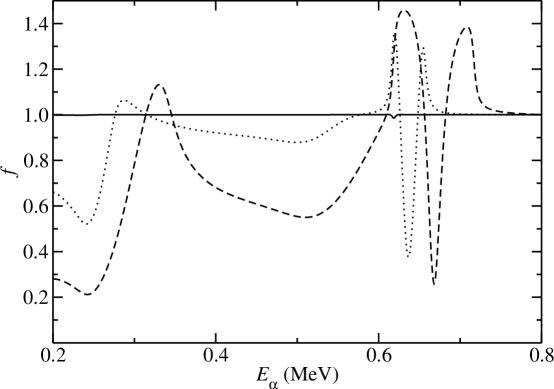
Figure 2: The correction factor $f$ for target 1 (solid curve), target 2 (dotted curve), and target 3 (dashed curve).

2.6 Discussion

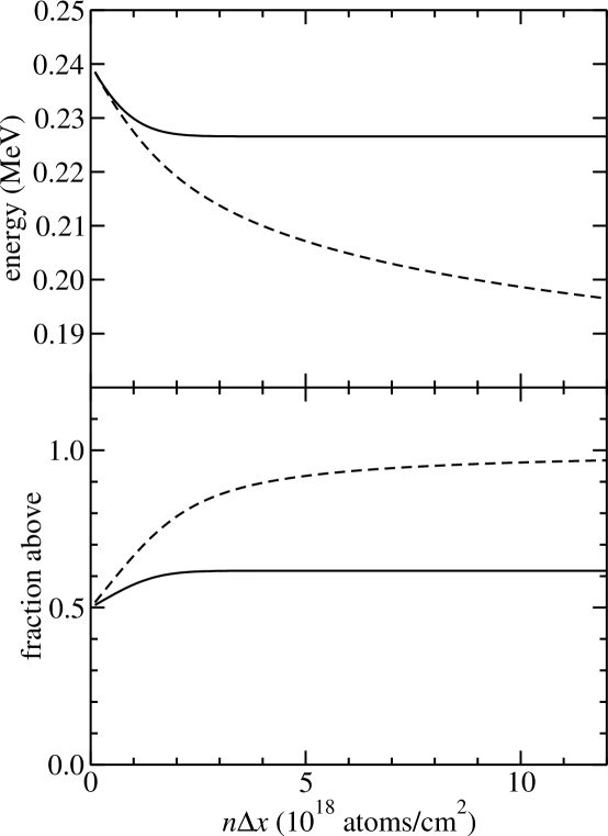
Figure 3: The dependence of the mean energy (solid curve) and effective energy (dashed curve) on the target thickness is shown in the upper panel, for ${}^{9}{\rm Be}(\alpha,n)$ and an incident $\alpha$ energy of 0.24 MeV. The lower panel shows the corresponding fractions of the yield resulting from reaction energies above the mean energy (solid curve) and above the effective energy (dashed curve).

It is found that there are many possible approaches to the energy deconvolution that are mathematically exact. However, in practice, these different choices may lead to different results, due to the fact that the energy dependence of the cross section and the nature of the energy convolution are not exactly known. It may also be the case in practice that approximate deconvolutions, such as ignoring the correction factor $f$, may provide perfectly acceptable results.

In the preliminary stages of the analysis of the data presented in Ref. [6], the effective energy approach described above was attempted. Two shortcomings of this method were encountered. The first problem is related to the fact that it requires inverting the cross section function. If the cross section has a local maxima or minima (e.g., at the peaks of or between resonances), this inversion is ambiguous. A criterion for selecting the solution must then be adopted; choosing the one nearest $E_{0}-\Delta E/2$ is one reasonable convention. In any case, one finds that $E_{\rm eff}(E_{0})$ is a discontinuous function and that certain ranges of $E_{\rm eff}$ cannot be reached for any $E_{0}$. Effectively, data points are pushed away in energy from cross section maxima or minima. The analytic approximation for the effective energy given by Eq. (12) is a quadratic equation and provides an example of this ambiguity. If the cross section has a local extrema at the center of the target, i.e., if $({\rm d}\sigma/{\rm d}E)_{E_{h}}=0$, then $E_{\rm eff}=E_{0}-\Delta E/2\pm\Delta E/\sqrt{12}$, and the choice of roots in ambiguous. In the case of resonances (maxima) this behavior was not deemed desirable because the presence of the resonance was largely responsible for the measured yield and one expects reasonable procedures to assign an energy to a measurement that reflects the reaction energies that gave rise to the measured yield.

Another shortcoming noted is that for thicker targets at energies well below the Coulomb barrier, $E_{\rm eff}$ is located at an energy significantly less than the energies where the majority of the yield is generated. In Fig. 3, the mean and effective energies are plotted versus the target thickness, for the ${}^{9}{\rm Be}(\alpha,n)$ reaction with an indicant $\alpha$ energy of 0.24 MeV (approximately the lowest energy measured in Ref. [6]). It is seen that the mean energy approaches a constant value once a thickness of $\approx 2\times 10^{18}$/cm² has been reached, as additional target thickness does not contribute to the integrals in Eq. (8). However, the effective energy continues to decrease as the target thickness is increased, as additional target thickness does continue to contribute to the integral on the left-hand side of Eq. (5). The lower panel of Fig. 3 shows the fraction of the yield resulting from reaction energies above mean and effective energies. It is seen that for the mean energy the fraction remains nearly one half, while for the case of the effective energy it approaches one. This behavior of the effective energy is not desirable, as the effective energy provides a misleading picture of what reaction energies were actually measured. In this situation the effective energy approach will also be more prone to systematic errors resulting from imprecise knowledge of the energy dependence of the cross section.

It was for the above reasons that the effective energy was not used by Wrean et al. [6]. Another situation where the effective energy approach is less useful is when multiple yields are analyzed from a single bombardment, such as for cross sections to different final states or differential cross sections for different angles. The energy dependences of these cross sections may be quite different, e.g., because of resonances involving particular partial waves, resulting in different effective energies being assigned to the different measurements. The resulting data are much more difficult to present and further analyze: consider, for example, an angular distribution where each angle corresponded to a different energy! This complication can be avoided via the mean or median energy approaches, using the total cross section to calculate the mean or median energy, and then applying the appropriate correction factors to the individual partial or differential cross sections. This approach is used below for the analysis of ${}^{12}{\rm C}(\alpha,\gamma){}^{16}{\rm O}$ angular distribution data.

The above difficulties with the effective energy method are related to the fact that all of the deconvolution is performed by adjusting the effective energy. These difficulties can be avoided by adopting alternative choices for the energy and determining the experimental cross section via Eqs. (6) and (7). Both the mean and median energies, defined by Eqs. (8) and (9), are reasonable choices that assign energies to the experimental cross section that accurately reflect the energies that were measured. We are not aware of any cases where there would be significant differences between these two approaches. We have a slight preference for the mean energy, as it is easier to calculate than the other energy definitions discussed here.

In all of this discussion, it has been assumed that the convolution kernel and the energy dependence of the cross section are known. In practice these inputs may not be precisely determined, and error analysis must be considered. For the cross section extraction, it has been found that using self-consistent iterative procedures to determine the energy dependence of the cross section work quite well in several cases; see, e.g., Wrean et al. [6], Lemut [1]. Uncertainties arising from the cross section assumptions and the possibility missing features in the cross section due to insufficient energy resolution must be considered. Particular attention should be paid to the lowest-energy cross section data point (or points), where the assumed energy dependence of the cross section is obviously not constrained by any lower-energy data points. In addition, the energy regions above strong resonances should be scrutinized for the possibility that a tail in the energy resolution function causes measurements above the resonances to receive resonant contributions. The latter effect is important in the case discussed in the following section.

3 Application to ${}^{12}{\rm C}(\alpha,\gamma){}^{16}{\rm O}$ data

Extensive angular distribution measurements of the ${}^{12}{\rm C}(\alpha,\gamma_{0}){}^{16}{\rm O}$ reaction were performed at Stuttgart a few years ago using detectors from the EUROGAM array [2, 15]. Measurements of this type are necessarily taken with targets which give rise to significant energy averaging effects. The energy deconvolution is complicated by the fact that the energy dependence of the differential cross section depends upon the angle, particularly near the $E_{c.m.}=2.68$-MeV resonance. In Refs. [2, 15], a complete energy deconvolution was not attempted. The primary goal of the present analysis is to more fully take into account the effects of energy averaging and to put the data into a form that is useful for further analyses, including a simultaneous $R$-matrix analysis of the angular distributions. New information about the interference structure involving the $E_{c.m.}=2.68$-MeV resonance [16] is taken into account.

3.1 Cross Section Model

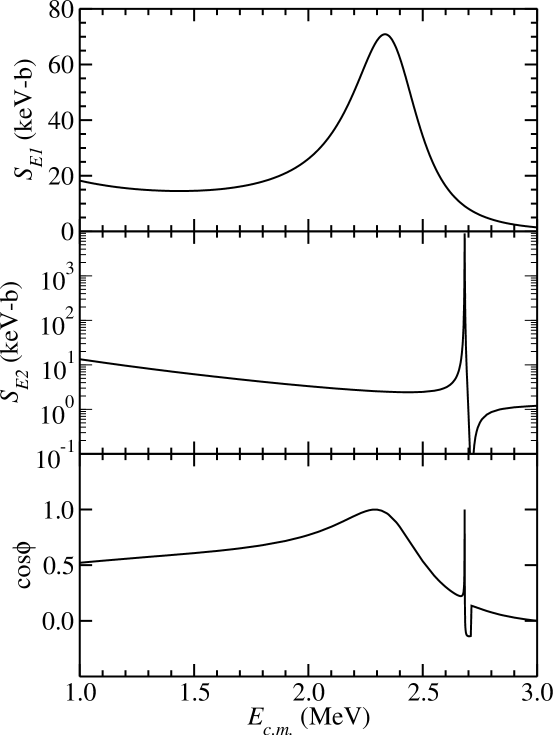
Figure 4: The $R$-matrix parametrizations for $S_{E1}$, $S_{E2}$, and $\cos\phi$ as a function of CM energy.

In order to consider the effects of energy convolution on the differential cross section, a model for its energy dependence must be adopted. The differential cross section for ${}^{12}{\rm C}(\alpha,\gamma_{0}){}^{16}{\rm O}$ can then be written as [3, 17]

$$\frac{{\rm d}\sigma}{{\rm d}\Omega} = \frac{1}{4\pi}\biggl{[}\sigma_{E1}(1-P_{2})+\sigma_{E2}(1+\frac{5}{7}P_{2}-\frac{12}{7}P_{4})$$ (18)

$$+6\cos\phi\sqrt{\frac{\sigma_{E1}\sigma_{E2}}{5}}(P_{1}-P_{3})\biggr{]},$$

where $\sigma_{E1}$ and $\sigma_{E2}$ are the $E1$ and $E2$ ground-state cross sections, $\phi$ is the relative phase, and the angular dependence is contained in the Legendre polynomials $P_{l}\equiv P_{l}(\cos\theta)$. The term $\propto\sqrt{\sigma_{E1}\sigma_{E2}}$ results from $E1$-$E2$ interference, and gives rise to an asymmetry around $90^{\circ}$ in the differential cross section. It is often convenient to to use the $S$-factors $S_{EL}=\sigma_{EL}E\exp(2\pi\eta)$, where $\eta$ is the Coulomb parameter. Equation (18) can also be written as

$$\frac{{\rm d}\sigma}{{\rm d}\Omega}=\frac{\sigma_{0}}{4\pi}W(\theta),\quad{\rm with}\quad W(\theta)=1+\sum_{l=1}^{4}a_{l}P_{l},$$ (19)

where $\sigma_{0}=\sigma_{E1}+\sigma_{E2}$,

$$a_{1}=-a_{3} = \frac{6\cos\phi}{\sigma_{0}}\sqrt{\frac{\sigma_{E1}\sigma_{E2}}{5}},$$ (20)

$$a_{2} = \frac{-7\sigma_{E1}+5\sigma_{E2}}{7\sigma_{0}},{\rm~{}and}$$ (21)

$$a_{4} = -\frac{12}{7}\frac{\sigma_{E2}}{\sigma_{0}}.$$ (22)

If the above theoretical expressions for the differential cross section are to be compared to experimental differential cross sections measured with a finite solid angle, $P_{l}$ should be replaced with $Q_{l}P_{l}$, where the $Q_{l}$ are the attenuation factors [18]. We will utilize $W_{Q}(\theta)$ and $W(\theta)$ to indicate angular dependences with and without the attenuation coefficients, respectively.

For computing the convolutions, we assume that $\sigma_{E1}$, $\sigma_{E2}$, and $\cos\phi$ are given by $R$-matrix parametrizations, as shown in Fig. 4, where for convenience $S$ factors are shown in place of cross sections. The $E1$ parametrization is essentially the same as that described in Ref. [19], except that more recent phase shift data [20] has been fitted. The $E2$ parametrization is taken from Ref. [16] (the solid curve in the lower panel of Fig. 2). The parametrization for $\cos\phi$ is taken from the relative phase of the above $E1$ and $E2$ parametrizations. It should be noted that $\cos\phi$ is primarily defined by the P- and D-wave scattering phase shifts [21] and that our parametrization accurately reproduces the recently-published phase shifts of Tischhauser et al. [20]. Many of the details of these parametrizations are unimportant for the convolutions discussed below. The essential ingredients are the roughly constant $S$-factors below $E_{c.m.}=2$ MeV, and the behavior of $\sigma_{E1}/\sigma_{E2}$ and $\cos\phi$ near the narrow $E_{c.m.}=2.68$-MeV resonance. This behavior is largely determined by the known resonance parameters, but the nature of the interference was until recently not understood [21]. However, the experiment and analysis of Sayre et al. [16] have now conclusively determined how this resonance interferes with other $E1$ and $E2$ amplitudes.

3.2 The Experimental Data

Refs. [2, 15] report measurements at 25 bombarding energies that are described in Tables I and II of Assunção et al. [2]; particular energies will be referred to by measurement numbers 1-25 which are ordered by energy as given in these tables. Gamma-ray angular distributions were measured at nine angles and are given in Figs. D.1-9 of Fey [15]. These data are the efficiency-corrected numbers of gamma rays detected, scaled by $10^{-4}$; these quantities are defined here to be $N_{\gamma}(\theta)$. The data have also been corrected for finite solid angle. When normalized by the factor $0.624(4\pi)Q\tilde{N}$, where $Q$ and $\tilde{N}$ are given in Table II of Ref. [2], these data become differential cross sections in nb/sr. We have verified that these differential cross sections, when fitted with Eq. (18), reproduce the cross sections and their uncertainties given in Table I of Ref. [2], for both the two-parameter and three-parameter approaches described therein. The phase $\phi$ and its error was also well reproduced in the case of the three-parameter fit. The fit was determined by $\chi^{2}$ minimization, with the parameter errors indicating the range of parameter values consistent with an increase in $\chi^{2}$ by an amount $\leq 1$ above the minimum when the remaining free parameters are varied. The uncertainty in $\tilde{N}$ is propagated after fitting the angular distributions. The uncertainty in center-of-mass (CM) energy, given in column 2 of Table I of Ref. [2], is propagated to the $S$ factors when calculating them from the cross section.

These fits also describe the reported angular distribution data via $N_{\gamma}(\theta)=N_{\gamma 0}W(\theta)$. We have removed the correction for finite solid from the data by the transformation $N_{\gamma}(\theta)\rightarrow N_{\gamma}(\theta)+N_{\gamma 0}[W_{Q}(\theta)-W(\theta)]$, where $N_{\gamma 0}$ and $\sigma_{E1}/\sigma_{E2}$ are taken from the two-parameter fit. This approach by construction ensures that the identical results will be produced when the modified $N_{\gamma}(\theta)$ is fitted with the attenuation coefficients taken into account. This step was taken because, in the simultaneous fits of multiple angular distributions, we feel it is not desirable to have already made corrections that are based on single-energy fits. It also makes it possible to investigate the effects of uncertainties in the $Q_{l}$. These factors are given in Ref. [2], having been calculated from a simple formula, their Eq. (4.2). We have calculated the $Q_{l}$ independently, using a geant4 simulation [22], taking into account the tapered geometry of the EUROGAM detectors [23, 24] and the angle-dependent detector distances (see Table 3.2 of Ref. [15]). The changes in the extracted cross sections from using our $Q_{l}$ were generally found to be negligible. The one exception was for the four $E1$ cross sections underlying the narrow $E2$ resonance (measurements 18-21). However, these four $E1$ cross sections also have very large statistical uncertainties, rendering the changes to be of less importance. We have thus used the $Q_{l}$ factors given in Ref. [2] in all subsequent analysis.

Although the “effective energy” is extensively discussed by Assunção et al. [2], Refs. [2, 15] do not explicitly state how it is defined. They presumably used what is called in this work the median energy, as that was utilized in a slightly earlier analysis by the same group; see Eqs. (3.19) and (3.20) of Ref. [25].

3.3 Center of Mass Motion

The analysis given in Refs. [2, 15] did not consider the effects of CM motion. We have included it in our analysis, using Eq. (B9) given by Brune [21]. This approach leads to a modified form for the angular distribution:

$$W_{Q\beta}(\theta)=P_{Q\beta 0}+\sum_{l=1}^{4}a_{l}P_{Q\beta l}(\cos\theta),$$ (23)

where

$$P_{Q\beta 0} \equiv 1+2\beta Q_{1}P_{1},$$ (24)

$$P_{Q\beta l} \equiv Q_{l}P_{l}+\frac{\beta}{2l+1}[(l+1)(l+2)Q_{l+1}P_{l+1}-l(l-1)Q_{l-1}P_{l-1}],$$

and $\beta$ is the speed of the recoiling ${}^{16}{\rm O}$ nucleus relative to the speed of light. We have utilized a value of 0.849 for the required $Q_{5}$ attenuation coefficient. The inclusion of these effects makes some non-negligible changes, particularly for the extracted $E2$ cross sections with $E_{c.m.}$ between 2.0 and 2.6 MeV, which are reduced by 10-15%. The reduction is very similar to the case reported in Ref. [21]. The effects of CM motion have been included for all analysis described below, with $\beta$ calculated for the median energies in the target reported by Ref. [2]. We have verified that this approximation (ignoring the energy dependence of $\beta$ over the beam-energy loss in the target) is excellent. It should be noted that the resulting formula for the differential cross section remains a linear combination of three terms proportional to $\sigma_{E1}$, $\sigma_{E2}$, and $\cos\phi\sqrt{\sigma_{E1}\sigma_{E2}}$. With the assumption of constant $\beta$, all of the energy dependence of the differential cross section is contained in these three quantities.

3.4 Energy Convolution Model

The targets consisted of ${}^{12}{\rm C}$ implanted into gold. The depth distribution can be described by $g(y)$, where $g$ is the ratio of ${}^{12}{\rm C}$ to $({}^{12}{\rm C}+{\rm Au})$ and $y$ measures the depth in units of $({}^{12}{\rm C}+{\rm Au})$ atoms/cm². Equation 2 becomes

$$Y(E_{\alpha})=\int_{0}^{y_{0}}\sigma(E(y))\,g(y)\,{\rm d}y,$$ (25)

where $E_{\alpha}$ is the incident $\alpha$ energy, $y_{0}$ is the maximum depth considered (where $g(y)\rightarrow 0$), and the variation of energy with depth is determined by solving the differential equation

$$\frac{{\rm d}E}{{\rm d}y}(y)=-g(y)\,\epsilon_{\rm C}(E)-[1-g(y)]\,\epsilon_{\rm Au}(E),$$ (26)

subject to $E(0)=E_{\alpha}$, where $\epsilon_{\rm C}$ and $\epsilon_{\rm Au}$ are the stopping powers for helium ions in carbon and gold, respectively [26]. The total number of carbon atoms per unit area in the distribution $g(y)$ is given by

$$\tilde{N}_{g}=\int_{0}^{y_{0}}g(y)\,{\rm d}y.$$ (27)

We have neglected energy straggling, as investigations into this process indicated that this effect is small compared to changes associated with uncertainties in $g(y)$. The calculated target-averaged differential cross section can thus be defined to be

$$\left\langle\frac{{\rm d}\sigma}{{\rm d}\Omega}\right\rangle=\frac{1}{\tilde{N}_{g}}\int_{0}^{y_{0}}\frac{{\rm d}\sigma}{{\rm d}\Omega}(E)\,g(y)\,{\rm d}y;$$ (28)

recall that the corresponding experimental value was noted in Subsec. 3.2 to be

$$\left\langle\frac{{\rm d}\sigma}{{\rm d}\Omega}\right\rangle_{\rm exp}=\frac{N_{\gamma}(\theta)}{0.624(4\pi)Q\tilde{N}}.$$ (29)

We have thus allowed for the possibility that $g(y)$ has a normalization that does not correspond to the experimentally-determined areal density of carbon, i.e., that $\tilde{N}\neq\tilde{N}_{g}$.

3.5 Three-Parameter Fits Near the Narrow $E2$ Resonance

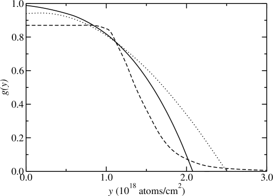
Figure 5: Depth profiles $g(y)$ for the targets used near the narrow $E2$ resonance. The before (solid curve) and after (dotted curve) profiles are taken from Fig. 8 of Ref. [2]. The dashed curve is discussed in the text.

We begin by considering measurements 13-25 which are near the narrow $E2$ resonance and were conducted with very similar targets. For bombarding energies at and above the resonance energy, the effects of energy convolution are substantial. At this stage, we will proceed by comparing measurements of the target-averaged cross sections to calculated convolutions, as opposed to proceeding straight to deconvolutions.

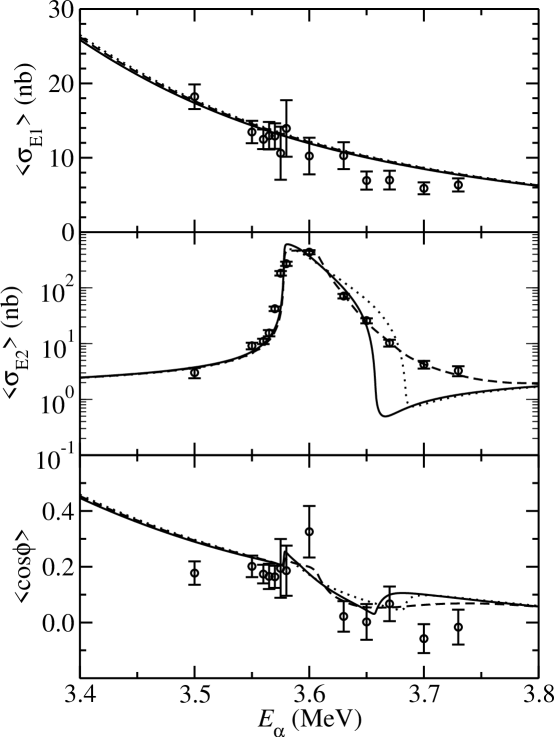
Figure 6: Results for the experimental and theoretical $\langle\sigma_{EL}\rangle$ and $\langle\cos\phi\rangle$ versus bombarding energy. The results from measurements 13-25 are shown as the circles and the theoretical calculations are shown as the curves, which correspond to the depth profiles shown in Fig. 5.

A three-parameter fit to the experimental target-averaged differential cross sections may now be performed using

$$\left\langle\frac{{\rm d}\sigma}{{\rm d}\Omega}\right\rangle_{\rm exp} = \frac{1}{4\pi}\biggl{[}\langle\sigma_{E1}\rangle(P_{Q\beta 0}-P_{Q\beta 2})+\langle\sigma_{E2}\rangle(P_{Q\beta 0}+\frac{5}{7}P_{Q\beta 2}-\frac{12}{7}P_{Q\beta 4})$$ (30)

$$+6\langle\cos\phi\rangle\sqrt{\frac{\langle\sigma_{E1}\rangle\langle\sigma_{E2}\rangle}{5}}(P_{Q\beta 1}-P_{Q\beta 3})\biggr{]},$$

to yield experimental values for $\langle\sigma_{E1}\rangle$, $\langle\sigma_{E2}\rangle$, and $\langle\cos\phi\rangle$. The theoretical expectations for these quantities are:

$$\langle\sigma_{EL}\rangle = \frac{1}{\tilde{N}_{g}}\int_{0}^{y_{0}}\sigma_{EL}\,g(y)\,{\rm d}y$$ (31)

$$\langle\cos\phi\rangle = \frac{1}{\tilde{N}_{g}\sqrt{\langle\sigma_{E1}\rangle\langle\sigma_{E2}\rangle}}\int_{0}^{y_{0}}\cos\phi\sqrt{\sigma_{E1}\sigma_{E2}}\,g(y)\,{\rm d}y,$$ (32)

where $L=1,2$ and the energy dependences of the cross sections and $\cos\phi$ under the integrals have been suppressed.

These measurements were carried out with targets containing approximately $1.3\times 10^{18}$ ${}^{12}{\rm C}$/cm². Example before-and-after depth profiles of such a target are given in Fig. 8 of Ref. [2] and are also shown in Fig. 5. The results for the experimental and theoretical $\langle\sigma_{EL}\rangle$ and $\langle\cos\phi\rangle$ are shown in Fig. 6. In addition to the two depth profiles from Ref. [2], we have considered a third profile that was adjusted to optimize the agreement with the experimental $\langle\sigma_{E2}\rangle$. We find that $\langle\sigma_{E1}\rangle$ is insensitive to the details of the depth profile for all energies considered. Below the resonance energy, $\langle\sigma_{E2}\rangle$ and $\langle\cos\phi\rangle$ are also insensitive to the details of the depth profile. However, at and above the resonance energy, $\langle\cos\phi\rangle$ and particularly $\langle\sigma_{E2}\rangle$ are very sensitive to the depth profile.

The third depth profile, shown by the dashed curves in Figs. 5 and 6, includes a small tail which extends beyond a depth of $2.5\times 10^{18}$ atoms/cm². It is this tail which allows the calculation to reproduce the two highest-energy data points. Note that the two depth profiles from Ref. [2] do not allow the resonance to contribute to the $\langle\sigma_{E2}\rangle$ calculation at the two highest energies. We believe that is extremely likely that $E2$ contribution for these data points is in fact coming from the resonance and the tail of the depth profile. The alternative explanation would be that our model cross section is too low at these energy by a factor of $\sim 5$, which is very unlikely (see Ref. [16]). In addition, the Rutherford backscattering technique, which was used to determine the depth profiles in Ref. [2], is not sensitive to a small tail. Further evidence for this interpretation is provided by the gamma-ray spectra given in Figs. C.24 and C.25 of Ref. [15] that correspond to these two data points. The full-energy peaks from the ${}^{12}{\rm C}(\alpha,\gamma_{0}){}^{16}{\rm O}$ reaction at angles away from $90^{\circ}$ are double-peaked. The lower-energy portions of the peaks match the peak energies for the on-resonance measurements, an observation consistent with significant reaction yield coming from the resonance.

We conclude that meaningful $E2$ cross section cannot be extracted for energies at and above the resonance energy ($E_{\alpha}=3.580$ MeV and higher) due to the strong sensitivity to the depth profile. Similar conclusions were reached by Assunção et al. [2], except that they extracted cross sections and $S$ factors for the two highest-energy measurements. For the reasons given in the previous paragraph, we do not believe these two points can be reliably analyzed. The $E1$ cross sections can separated from the uncertain $E2$ contribution using the above three-parameter fit procedure; the $\langle\sigma_{E1}\rangle$ will be analyzed further below.

3.6 Deconvolution of the Angular Distributions

Figure 7: The depth profile $g(y)$ for measurements 1-10.

The depth profiles utilized in the analysis were defined as follows. For measurements 1-10, which utilized relatively thick targets, we have assumed the depth profile shown in Fig. 7. In Ref. [2], median energies were determined using the assumption of a constant $S$ factor. We have determined the over all scale of these depth profiles by adjusting the maximum depth $y_{0}$ to reproduce the the median energies given by Ref. [2], where we have, for this part of the calculation only, assumed a constant $S$ factor in order to reproduce the methods of Ref. [2]. It should be noted that this procedure generates depth profiles with ${}^{12}{\rm C}$ areal densities that agree with those given in Table II of Ref. [2] to better than 10%. For measurements 11-25, which utilized relatively thinner targets, we have assumed the depth profile shown by the dashed curve in Fig. 5. In these cases, the depth scale of each profile has been scaled by $\tilde{N}/1.30$ so that it reproduces the experimental carbon areal density.

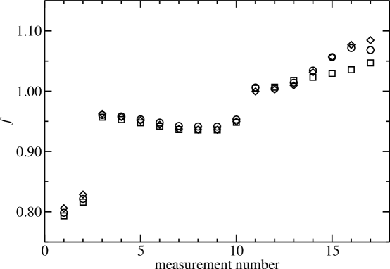
Figure 8: The calculated correction factors for $48^{\circ}$ (circles) $90^{\circ}$ (squares), and $130^{\circ}$ (diamonds) versus measurement number, for measurements 1-17.

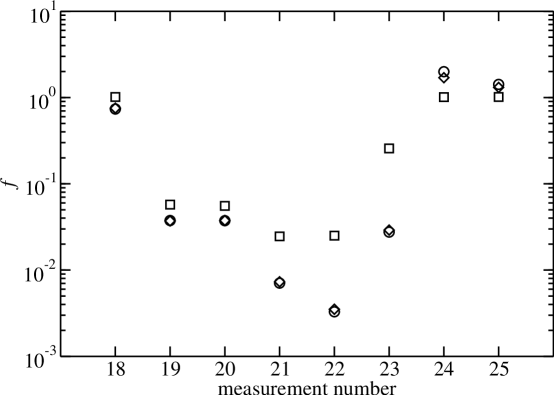
Figure 9: The calculated correction factors for $48^{\circ}$ (circles) $90^{\circ}$ (squares), and $130^{\circ}$ (diamonds) versus measurement number, for measurements 18-25.

In order to minimize the number of changes in the analysis relative to Ref. [2], the angular distributions will be referenced to the median energy. The depth of the median energy is defined by

$$\int_{0}^{y_{0}}\sigma_{0}(E(y))\,g(y)\,{\rm d}y=2\int_{0}^{y_{m}}\sigma_{0}(E(y))\,g(y)\,{\rm d}y,$$ (33)

where $y_{m}$ is the median depth and the median energy is given by $E_{m}=E(y_{m})$. Note also that we have utilized the total ground state cross section in the definition. The deconvoluted differential cross sections, referenced to the median energies defined above, are calculated from the experimental target-averaged differential cross sections (defined by Eq. 29) via

$$\left(\frac{{\rm d}\sigma}{{\rm d}\Omega}\right)_{\rm exp}=\frac{1}{f}\left\langle\frac{{\rm d}\sigma}{{\rm d}\Omega}\right\rangle_{\rm exp},$$ (34)

where the correction factor is given by

$$f=[\tilde{N}_{g}\frac{{\rm d}\sigma}{{\rm d}\Omega}(E_{m})]^{-1}\int_{0}^{y_{0}}\frac{{\rm d}\sigma}{{\rm d}\Omega}(E)\,g(y)\,{\rm d}y.$$ (35)

The theoretical form assumed for the differential cross section is the same as used in Subsec. 3.5:

$$\frac{{\rm d}\sigma}{{\rm d}\Omega}(E)=\frac{\sigma_{0}}{4\pi}W_{Q\beta}(\theta).$$ (36)

The resulting correction factors are shown in Figs. 8 and 9 for three representative angles. For measurements 1-17 (below the peak of the narrow $E2$ resonance), the correction factors are seen to differ from unity by at most 20% and to depend very little upon the angle. For measurements 18-25, the correction factors show much great departures from unity and significant angular dependence; these correction factors are also very sensitive to the assumed target depth profile.

At this point, it is instructive to investigate how sensitive the deconvolution is to the assumed form of the cross section and depth profiles, both through the calculation of the median energy and the correction factor $f$. We will limit our consideration here to measurements 1-13, as measurements 14-17 are on the rising slope of the narrow $E2$ resonance where taking the exact energy dependence of this resonance into account is clearly important, and it has already been noted that the measurements 18-25 are very sensitive to the assumed depth profile. To test the sensitivity to the assumed cross section, we have repeated the deconvolution assuming a constant $S$-factor and $\cos\phi$. In the case of the median energy, only measurements 1-2 show any sensitivity: the calculation with our model cross section yields median energies about 7-keV lower than the constant $S$-factor calculation; note that this lowering corresponds to a a 4% increase in the calculated experimental $S$ factors. The differences in the calculated correction factors are at most 5%. We have also investigated the effects of a 20% increase in the scale of the depth profiles. This change leads to reductions in the median energy of up to 12 keV and up to 9% reductions in the correction factor. All these changes are within the tolerance implied by the uncertainties assigned to the effective energies given in column 2 of Table II of Ref. [2].

Figure 10: The $E1$ (upper panel) and $E2$ (lower panel) $S$ factors. The values determined from the deconvoluted differential cross sections for measurements 1-17 are given as circles. The corresponding values given by Ref. [2] are given as squares; the error bars for these points are not shown but are essentially identical to the error bars on the corresponding circles. The $R$-matrix parametrizations are given by the solid curves.

The deconvoluted experimental differential cross sections for measurements 1-17 have been fitted using

$$\left(\frac{{\rm d}\sigma}{{\rm d}\Omega}\right)_{\rm exp} = \frac{1}{4\pi}\biggl{[}\sigma_{E1}(P_{Q\beta 0}-P_{Q\beta 2})+\sigma_{E2}(P_{Q\beta 0}+\frac{5}{7}P_{Q\beta 2}-\frac{12}{7}P_{Q\beta 4})$$ (37)

$$+6\cos\phi\sqrt{\frac{\sigma_{E1}\sigma_{E2}}{5}}(P_{Q\beta 1}-P_{Q\beta 3})\biggr{]},$$

to determine $\sigma_{E1}$ and $\sigma_{E2}$; $\cos\phi$ has been fixed at the value given by the $R$-matrix parametrization shown in Fig. 4. The fit was determined by $\chi^{2}$ minimization, with the parameter errors indicating the range of parameter values consistent with an increase in $\chi^{2}$ by an amount $\leq 1$ above the minimum when the remaining free parameters are varied. The uncertainties in $\tilde{N}$ and the CM energy have been propagated after fitting. The results are shown as $S$-factors in Figs. 10 and 11 and Table 1. For reference, the figures also show results given by Ref. [2] from the analysis of the same raw data and the $R$-matrix parametrization shown in Fig. 4. Our analysis differs from that given in Ref. [2] in three ways: the effects of CM motion have been taken into account, the median energy has been calculated using a more accurate representation of the energy dependence of the cross section, and the differential cross sections have been adjusted by the the correction factor given by Eq. 35. Another difference is that we are fitting differential cross sections that have not been corrected for detector solid angle effects but rather include these corrections in our fitting function; this difference should not change the extracted $S$ factors. The differences between our results and those given by Ref. [2] are generally quite small. In the case of the $E2$ $S$ factor, the effects of CM motion and the deconvolution tend to cancel, leading to very small changes. Our results are also in generally good agreement with the $R$-matrix parametrization, which indicates consistency between the data and our cross section model. Near the narrow $E2$ resonance, Ref. [2] provided two values of the energy (columns 2 and 3 of Table II of that reference); both values are plotted in Fig. 11. We note that for measurements 14-17, both our results and those of Ref. [2] lie 3-10 keV to the left of the $R$-matrix parametrization. This discrepancy is also seen in Fig. 6. The $R$-matrix parametrizaton should be well determined here by the known parameters of the resonance. One possibility is that uncertainty in the beam energy contributes to this difference. In any case, the deconvolution procedure for measurements 14-17 must be viewed with some skepticism due to the lack of agreement between the resulting data points and our cross section model.

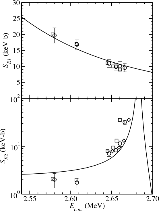
Figure 11: The $E1$ (upper panel) and $E2$ (lower panel) $S$ factors. The values determined from the deconvoluted differential cross sections for measurements 12-17 are given as circles. The corresponding values given by Ref. [2] using their energy method (I) are given as squares and for measurements 14-17 using their energy method (II) are as diamonds (shown only for the lower panel); the error bars for these points are not shown but are essentially identical to the error bars on the corresponding circles. The respective $R$-matrix parametrizations are given by the solid curves.

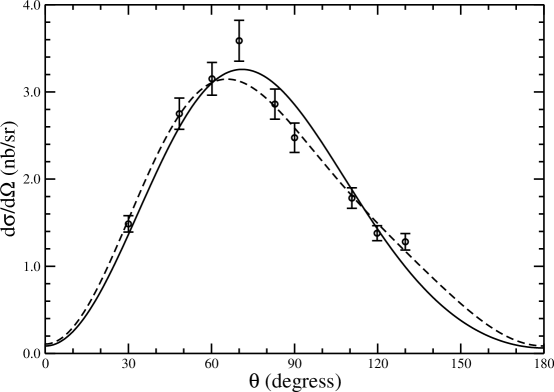
Figure 12: The deconvoluted angular distribution data for measurement 7. The solid and dashed curves show the two-parameter and three-parameter fits that are discussed in more detail in the text.

In Fig. 12, we show the differential cross section obtained for measurement 7, for which we find median energy to be $E=2.199$ MeV in the CM system. The two-parameter fit is shown as the solid curve; this fit utilized a fixed value of $\cos\phi=0.941$ and yields $\sigma_{E1}=24.3(5)$ nb and $\sigma_{E2}=0.8(1)$ nb with $\chi^{2}=22.0$. Assunção et al. [2] noted that three-parameter fits, where $\cos\phi$ was allowed to vary, tended to differ significantly from two-parameter fits for CM energies between 2.0 and 2.4 MeV. We find similar results. Such a three parameter fit for measurement 7 is also shown in Fig. 12 as the dashed curve; it yields $\sigma_{E1}=21.9(8)$ nb, $\sigma_{E2}=3.2(6)$ nb, and $\cos\phi=0.49(6)$ with $\chi^{2}=8.3$. The above uncertainties do not include the contribution from $\tilde{N}$ which is common to all angles of a single angular distribution. It is seen that while both fits give essentially identical total ground-state cross sections ($\sigma_{0}=\sigma_{E1}+\sigma_{E2}$), the three-parameter fit gives a much larger $\sigma_{E2}$ – by a factor of 3.8 which corresponds to 3.6 standard deviations. We would like to emphasize that there is no known reason for the value for $\cos\phi$ assumed in the two-parameter fit to be incorrect (see discussion in Ref. [21]). We have investigated the possible role of uncertainties in the deconvolution procedure on this finding. We conclude that it cannot be explained by this consideration, due to the lack of angle dependence of the convolution factor in this energy range (see Fig. 8). The most likely explanation is that angular distribution data contain unidentified systematic errors. Evidence for this explanation is provided by the $\chi^{2}$ values from both the two-parameter and three-parameter fits to the data. Our $\chi^{2}$ values are very similar to those of Ref. [2]; as can be seen from Table I of Ref. [2], the $\chi^{2}$ values always exceed the number of degrees of freedom and often do so by a substantial amount. Another observation is that particular angles show systematic deviations from the fits. For example, the $130^{\circ}$ data point lies above the fitted curve for 23 out of the 25 distributions in the case of the three-parameter fits (data near the narrow $E2$ resonance discussed in Subsec. 3.5 were also considered).

	$E_{\rm c.m.}$	$S_{E1}$	$S_{E2}$	$S_{0}$	$E_{c.m.}$	$S_{E1}$
	(MeV)	(keV-b)	(keV-b)	(keV-b)	(MeV)	(keV-b)
1	1.299	20.8(85)	4.3(54)	25.1(73)
2	1.337	14.5(59)	11.0(51)	25.5(69)
3	1.667	20.5(34)	4.8(12)	25.3(39)
4	1.969	26.5(39)	3.6(7)	30.1(43)
5	2.045	30.1(44)	3.9(7)	34.1(49)
6	2.123	41.5(60)	2.5(5)	44.0(63)
7	2.199	57.6(82)	2.0(4)	59.5(84)
8	2.236	61.1(86)	2.2(4)	63.3(89)
9	2.272	79.0(110)	2.9(5)	81.9(114)
10	2.343	71.0(99)	1.5(3)	72.6(101)
11	2.454	43.8(31)	2.3(4)	46.1(32)
12	2.580	19.7(24)	2.0(7)	21.7(25)
13	2.608	16.8(15)	1.8(4)	18.6(16)
14	2.647	10.9(12)	7.1(10)	18.0(16)	2.645	10.9(12)
15	2.655	9.9(11)	8.2(10)	18.1(16)	2.653	10.0(11)
16	2.660	10.1(15)	11.4(15)	21.5(20)	2.656	10.3(15)
17	2.666	9.6(13)	31.5(30)	41.1(36)	2.660	10.2(14)
18					2.664	8.3(28)
19					2.668	10.8(29)
20					2.683	7.7(19)
21					2.706	7.4(13)
22					2.721	4.8(9)
23					2.736	4.8(9)
24					2.759	3.8(5)
25					2.781	4.0(5)

Table 1: The deconvoluted $S$-factor data. The first column supplies the measurement number. The following four columns provide the $E1$, $E2$, and total $S$-factor data from the two-parameter fits discussed in Subsec. 3.6. The final two columns provide the $E1$ $S$-factor data from the three-parameter fits discussed in Subsec. 3.7.

In Table 1 we also provide the total ground-state $S$ factors $S_{0}$, where the uncertainty is determined using two-parameter fits considering $\sigma_{0}$ and $\sigma_{E2}/\sigma_{E1}$ to be independent variables. The uncertainties in $\tilde{N}$ and the CM energy have again been propagated after fitting. In a simultaneous $R$-matrix analysis of data from this experiment, we envision fitting fitting $S_{0}$ and the angular distributions. The angular distributions would be considered to be un-normalized, with the normalization carried in the $S_{0}$ data, and an overall normalization uncertainty of 9% would also be assumed for the entire data set (inferred from Table 5.2 of Ref. [15]). This approach ensures that only independent data with independent uncertainties are fitted; this would not be the case if both the $S_{E1}$ and $S_{E2}$ values were included in the fit.

3.7 Deconvolution of $E1$ data

In Subsec. 3.5 it was noted that target-averaged $E1$ cross sections can be extracted independently of the $E2$ cross sections. This analysis will be pursued further here, as it is useful for the data near the narrow $E2$ resonance where the $E2$ contribution is extremely sensitive to the assumed target profile. In this case, we define the median energy using the $E1$ cross section:

$$\int_{0}^{y_{0}}\sigma_{E1}(E(y))\,g(y)\,{\rm d}y=2\int_{0}^{y_{m}}\sigma_{E1}(E(y))\,g(y)\,{\rm d}y,$$ (38)

where the median energy is given by $E_{m}=E(y_{m})$. This procedure avoids introducing un-needed uncertainty through $E2$ contribution. The same target profiles are used as in Subsec. 3.6. The target-averaged $E1$ cross sections $\langle\sigma_{E1}\rangle$ are obtained using three-parameter fits to Eq. (30). Deconvoluted $E1$ cross sections are obtained via

$$(\sigma_{E1})_{\rm exp}=\frac{1}{f_{E1}}\langle\sigma_{E1}\rangle$$ (39)

where in this case the correction factor is given by

$$f_{E1}=[\tilde{N}_{g}\sigma_{E1}(E_{m})]^{-1}\int_{0}^{y_{0}}\sigma_{E1}(E)\,g(y)\,{\rm d}y.$$ (40)

The resulting $E1$ $S$ factors for measurements 14-25 are given in Table 1.

3.8 Electronic Files

Three supplementary files accompany this paper on the publisher’s website. These files contain the $N_{\gamma}(\theta)$ data from Ref. [15], the $N_{\gamma}(\theta)$ data with the correction for finite solid angle removed, and the $N_{\gamma}(\theta)$ data with the correction for finite solid angle removed and the deconvolution factor given by Eq. (35) applied, respectively. The latter data, when normalized by $0.624(4\pi)Q\tilde{N}$, become the deconvoluted experimental differential cross sections in nb/sr.

4 Conclusions

A general framework for deconvoluting the effects of energy averaging on charged-particle reaction measurements has been presented. There are many potentially correct approaches to the problem; the relative merits of some of them have been discussed.

These deconvolution methods have been applied to recent ${}^{12}{\rm C}(\alpha,\gamma){}^{16}{\rm O}$ measurements [2, 15]. This analysis has clarified what can, and what cannot, be explained by energy convolution effects. Very significant effects are found at and above the narrow 2.68-MeV resonance. Below this resonance, we find that considerations of energy deconvolution, as well as special relativity, lead to relatively small changes in the extracted $S$ factors. We have also extracted deconvoluted differential cross sections from this experiment. We expect that these results will be useful for future analyses, including a simultaneous $R$-matrix of the angular distributions.

References

- Lemut [2008] A. Lemut, Eur. Phys. J. A 36 (2008) 233.
- Assunção et al. [2006] M. Assunção, M. Fey, A. Lefebvre-Schuhl, J. Kiener, V. Tatischeff, J. W. Hammer, C. Beck, C. Boukari-Pelissie, A. Coc, J. J. Correia, S. Courtin, F. Fleurot, E. Galanopoulos, C. Grama, F. Haas, F. Hammache, F. Hannachi, S. Harissopulos, A. Korichi, R. Kunz, D. LeDu, A. Lopez-Martens, D. Malcherek, R. Meunier, T. Paradellis, M. Rousseau, N. Rowley, G. Staudt, S. Szilner, J. P. Thibaud, J. L. Weil, Phys. Rev. C 73 (2006) 055801.
- Dyer and Barnes [1974] P. Dyer, C. A. Barnes, Nucl. Phys. A233 (1974) 495.
- Filippone et al. [1983] B. W. Filippone, A. J. Elwyn, C. N. Davids, D. D. Koetke, Phys. Rev. C 28 (1983) 2222.
- Imbriani et al. [2005] G. Imbriani, H. Costantini, A. Formicola, A. Vomiero, C. Angulo, D. Bemmerer, R. Bonetti, C. Broggini, F. Confortola, P. Corvisiero, J. Cruz, P. Descouvemont, Z. Fülöp, G. Gervino1, A. Guglielmetti, C. Gustavino, G. Gyürky, A. P. Jesus, M. Junker, J. N. Klug, A. Lemut, R. Menegazzo, P. Prati, V. Roca, C. Rolfs, M. Romano, C. Rossi-Alvarez, F. Schümann, D. Schürmann, E. Somorjai, O. Straniero, F. Strieder, F. Terrasi, H. P. Trautvetter, Eur. Phys. J. A 25 (2005) 455.
- Wrean et al. [1994] P. R. Wrean, C. R. Brune, R. W. Kavanagh, Phys. Rev. C 49 (1994) 1205.
- Dwarakanath [1974] M. R. Dwarakanath, Phys. Rev. C 9 (1974) 805.
- Alexander et al. [1984] T. K. Alexander, G. C. Ball, W. N. Lennard, H. Geissel, H. B. Mak, Nucl. Phys. A427 (1984) 526.
- Brune et al. [1994] C. R. Brune, R. W. Kavanagh, C. Rolfs, Phys. Rev. C 50 (1994) 2205.
- King et al. [1994] J. D. King, R. E. Azuma, J. B. Vise, J. Görres, C. Rolfs, H. P. Trautvetter, A. E. Vlieks, Nucl. Phys. A567 (1994) 354. The information given in Table 3 of this reference could in principle be used to demonstrate some of the ideas presented in the present work. However, the reported target energy thickness decreases with decreasing proton energy, opposite from what one expects from the energy dependence of the stopping power. Further analysis was not pursued because of this inconsistency.
- Rolfs et al. [1987] C. Rolfs, H. P. Trautvetter, W. S. Rodney, Rep. Prog. Phys. 50 (1987) 233.
- Rolfs and Rodney [1988] C. E. Rolfs, W. S. Rodney, Cauldrons in the Cosmos, University of Chicago Press, Chicago, 1988.
- Iliadis [2007] C. Iliadis, Nuclear Physics of Stars, Wiley, Weinheim, 2007.
- Makii et al. [2009] H. Makii, Y. Nagai, T. Shima, M. Segawa, K. Mishima, H. Ueda, M. Igashira, T. Ohsaki, Phys. Rev. C 80 (2009) 065802. The right hand side of Eq. (3) of this reference appears to be missing a multiplicative factor of .
- Fey [2004] M. Fey, Im Brennpunkt der Nuklearen Astrophysik: Die Reaktion , Ph.D. thesis, Universität Stuttgart, 2004.
- Sayre et al. [2012] D. B. Sayre, C. R. Brune, D. E. Carter, D. K. Jacobs, T. N. Massey, J. E. O’Donnell, Phys. Rev. Lett. 109 (2012) 142501.
- Barker and Kajino [1992] F. C. Barker, T. Kajino, Aust. J. Phys. 44 (1992) 369.
- Rose [1953] M. E. Rose, Phys. Rev. 91 (1953) 610.
- Brune et al. [1999] C. R. Brune, W. H. Geist, R. W. Kavanagh, K. D. Veal, Phys. Rev. Lett. 83 (1999) 4025.
- Tischhauser et al. [2009] P. Tischhauser, A. Couture, R. Detwiler, J. Görres, C. Ugalde, E. Stech, M. Wiescher, M. Heil, F. Käppeler, R. E. Azuma, L. Buchmann, Phys. Rev. C 79 (2009) 055803.
- Brune [2001] C. R. Brune, Phys. Rev. C 64 (2001) 055803.
- Agostinelli et al. [2003] S. Agostinelli, J. Allison, K. Amako, J. Apostolakis, H. Araujo, P. Arce, M. Asai, D. Axen, S. Banerjee, G. Barrand, F. Behner, L. Bellagamba, J. Boudreau, L. Broglia, A. Brunengo, H. Burkhardt, S. Chauvie, J. Chuma, R. Chytracek, G. Cooperman, G. Cosmo, P. Degtyarenko, A. Dell’Acqua, G. Depaola, D. Dietrich, R. Enami, A. Feliciello, C. Ferguson, H. Fesefeldt, G. Folger, F. Foppiano, A. Forti, S. Garelli, S. Giani, R. Giannitrapani, D. Gibin, J. J. G. Cadenas, I. Gonzàlez, G. G. Abril, G. Greeniaus, W. Greiner, V. Grichine, A. Grossheim, S. Guatelli, P. Gumplinger, R. Hamatsu, K. Hashimoto, H. Hasui, A. Heikkinen, A. Howard, V. Ivanchenko, A. Johnson, F. W. Jones, J. Kallenbach, N. Kanaya, M. Kawabata, Y. Kawabata, M. Kawaguti, S. Kelner, P. Kent, A. Kimura, T. Kodama, R. Kokoulin, M. Kossov, H. Kurashige, E. Lamanna, T. Lampèn, V. Lara, V. Lefebure, F. Lei, M. Liendl, W. Lockman, F. Longo, S. Magni, M. Maire, E. Medernach, K. Minamimoto, P. M. de Freitas, Y. Morita, K. Murakami, M. Nagamatu, R. Nartallo, P. Nieminen, T. Nishimura, K. Ohtsubo, M. Okamura, S. O’Neale, Y. Oohata, K. Paech, J. Perl, A. Pfeiffer, M. G. Pia, F. Ranjard, A. Rybin, S. Sadilov, E. D. Salvo, G. Santin, T. Sasaki, N. Savvas, Y. Sawada, S. Scherer, S. Sei, V. Sirotenko, D. Smith, N. Starkov, H. Stoecker, J. Sulkimo, M. Takahata, S. Tanaka, E. Tcherniaev, E. S. Tehrani, M. Tropeano, P. Truscott, H. Uno, L. Urban, P. Urban, M. Verderi, A. Walkden, W. Wander, H. Weber, J. P. Wellisch, T. Wenaus, D. C. Williams, D. Wright, T. Yamada, H. Yoshida, D. Zschiesche, Nucl. Instrum. and Meth. in Phys. Res. A 506 (2003) 250.
- Nolan and the U. K.-FRANCE EUROGAM Collaboration [1990] P. J. Nolan, the U. K.-FRANCE EUROGAM Collaboration, Nucl. Phys. A520 (1990) 657c.
- Beausang et al. [1992] C. W. Beausang, S. A. Forbes, P. Fallon, P. J. Nolan, P. J. Twin, J. N. Mo, J. C. Lisle, M. A. Bentley, J. Simpson, F. A. Beck, D. Curien, G. deFrance, G. Duchêne, D. Popescu, Nucl. Instrum. and Meth. in Phys. Res. A 313 (1992) 37.
- Kunz [2002] R. W. Kunz, – Die Schlüsselreaktion im Heliumbrennen der Sterne, Ph.D. thesis, Universität Stuttgart, 2002.
- Ziegler et al. [2008] J. F. Ziegler, M. D. Ziegler, J. P. Biersack, computer code srim-2006, version 2008.4, 2008. URL: http://www.srim.org/.