Statistical Properties of Microstructure Noise

Abstract

We study the estimation of moments and joint moments of microstructure noise. Estimators of arbitrary order of (joint) moments are provided, for which we establish consistency as well as central limit theorems. In particular, we provide estimators of auto-covariances and auto-correlations of the noise. Simulation studies demonstrate excellent performance of our estimators even in the presence of jumps and irregular observation times. Empirical studies reveal (moderate) positive auto-correlation of the noise for the stocks tested.

Keywords: market microstructure noise, high frequency data, joint moments, auto-covariance, auto-correlation

1 Introduction

It has long been recognized that market microstructure noise plays a significant role in financial markets. See, for example, the seminal paper of Black (1986) and comprehensive reviews of Madhavan (2000), O’Hara (2003), Stoll (2003) and Hasbrouck (2007), among others. The market microstructure noise is induced by various frictions in the trading process. Examples of such frictions include bid-ask spread, asymmetric information of traders, the discreteness of price change, etc.

With the increasing availability of high frequency data, the market microstructure noise has received growing attention. Despite the small size, market microstructure noise accumulates at high frequency and affects badly the inferences about the efficient price processes, such as the estimation of volatilities. No-arbitrage based arguments (see, for example, Delbaen and Schachermayer (1994)) suggests that the (efficient) price processes should normally be semimartingales. The fundamental properties of semimartingales allow to make accurate inferences about volatilities and other quantities with high frequency observations. See, for example, Jacod and Protter (1998), Mykland and Zhang (2006), among others. However, for liquidly traded securities, empirical evidence such as the signature plots of Andersen et al. (2000) show clear noise accumulation effect at high frequency. Therefore, more recent research carefully analyzes both components of the market price processes: the latent semimartingale price process and the noise process.

Several methods to de-noise the data in the context of volatility estimation have been proposed. For example, the two-scale method as in Zhang et al. (2005), Aït-Sahalia et al. (2005); the kernel method as in Barndorff-Nielsen et al. (2008), Barndorff-Nielsen et al. (2011); the pre-averaging method as in Jacod et al. (2009), Kinnebrock et al. (2010); the multi-scale method as in Zhang (2006); the quasi-maximum likelihood method as in Xiu (2010), Aït-Sahalia et al. (2010), among others. These methods are shown to be very effective when the noise is an additive white noise, or presents some kind of independence between successive observation times. Gloter and Jacod (2001), Li and Mykland (2007) and Rosenbaum (2009) studied the case when the noise is of specific form such as round-off errors or round-off errors on top of additive white noise. On the other hand, Hansen and Lunde (2006) and Ukabata and Oya (2009) have shown evidence of dependence of the noise in financial markets. When there is autocorrelation in the data, one possible way to reduce the impact of dependence is to use subsampling and averaging. Hansen and Lunde (2006), Barndorff-Nielsen et al. (2008) and Aït-Sahalia et al. (2011) provide estimators when the noise satisfy certain weak dependence assumptions. However, the optimal subsampling scheme and de-noise method depend on the dependence structure. Hence understanding the dependence structure of the noise is essential for inferences.

Can we understand better the statistical properties of the noise? Specifically, for a particular security price process, how is the noise distributed and what is the dependence structure?

In this article we study how to estimate the moments and joint moments of the noise, based on high-frequency data. More specifically, under both settings where the observation times are equally spaced or are irregularly spaced, we propose estimators for (joint) moments of arbitrary orders of the noise. We establish consistency as well as central limit theorems for our estimators under certain mild mixing conditions on the noise (see Assumptions (NO-1) and (NO-2) below for precise statements). As is well known that under appropriate conditions on the tail any distribution can be fully reconstructed from its moments, our results allow one to understand the marginal distribution as well as the joint distributions of the noise.

Simple applications of our results include estimating the auto-covariances and auto-correlations of the noise. And as central limit theorems are available, one can readily build tests for testing, for example, whether auto-correlations of particular orders vanish or not.

The paper is organized as follows. Section 2 introduces the setting and assumptions. Section 3 presents the consistency and asymptotic normality results of our proposed estimators for the (joint) moments of the noise. Section 4 demonstrates our results via simulations. Empirical studies are carried out in Section 5 in which we show by estimation and hypothesis testing that the noises are (moderately) positively auto-correlated for the stocks tested. Section 6 concludes. The proofs are given in the Appendix A.

2 Setting and assumptions

In this paper, we have three basic ingredients. The first one is the underlying process $X$, typically the log-price of an asset; the second one is the observation scheme, the third one is the noise.

The assumptions on $X$ are the standard ones in this kind of problem, namely is an Itô semimartingale, possibly discontinuous, plus some mild additional assumptions : so $X$ is defined on some filtered probability space $(\Omega,\mathcal{F},(\mathcal{F}_{t})_{t\geq 0},\mathbb{P})$, and it admits the following Grigelionis representation:

$$X_{t}=X_{0}+\int_{0}^{t}b_{s}ds+\int_{0}^{t}\sigma_{s}dW_{s}+(\delta 1_{\{|\delta|\leq 1\}})\star(p\!\!\!\!{}_{{}_{=}}\,-q\!\!\!{}_{{}_{=}}\,)_{t}+(\delta 1_{\{|\delta|>1\}})\star p\!\!\!\!{}_{{}_{=}}\,{}_{t}.$$ (2.1)

In this formula, $W$ is a standard Brownian motion, and $p\!\!\!\!{}_{{}_{=}}\,$ is a Poisson random measure on $\mathbb{R}_{+}\times E$, where $(E,\mathcal{E})$ is a Polish space, with a non-random intensity measure of the form $q\!\!\!{}_{{}_{=}}\,(dt,dz)=dt\otimes\lambda(dz)$ with $\lambda$ a $\sigma$-finite measure on $(E,\mathcal{E})$. The above is the general form of an Itô semimartingale, and we assume the following on the optional coefficients $b$ and $\sigma$ and the predictable coefficient $\delta=\delta(\omega,t,z)$:

Assumption (H): The process $b$ is locally bounded, the process $\sigma$ is càdlàg, and there is a localizing sequence $(\tau_{n})$ of stopping times and, for each $n$, a deterministic  nonnegative function $J_{n}$ on $E$ satisfying $\int\!J_{n}(z)^{2}\,\lambda(dz)<\infty$ and such that $|\delta(\omega,t,z)|\wedge 1\leq J_{n}(z)$ for all $(\omega,t,z)$ with $t\leq\tau_{n}(\omega)$.

Next, we describe how observations take place. At stage $n$, that is for a given frequency of observations, the successive observations occur at times $0=T(n,0)<T(n,1)<\cdots$, for a sequence $T(n,i)$ of (possibly random) finite times increasing to $\infty$ as $i\to\infty$, so the number of observations up to time $t$ is $N_{n}(t)+1$, where $N_{n}(t)=\sup(i:T(n,i)\leq t)$. The minimal assumption on the observation times is that each $T(n,i)$ is a stopping time, and the mesh goes to $0$ in a sense specified later, as $n\to\infty$. Moreover, at time $T(n,i)$ the process $X$ is contaminated by some noise, meaning that we observe the variable

$$Y^{n}_{i}=X_{T(n,i)}+\varepsilon^{n}_{i},$$ (2.2)

where the noise is $\varepsilon^{n}_{i}$.

For the sake of motivation about our forthcoming assumptions, we (temporarily) suppose that the noise is independent of $X$, centered, stationary, and with a negative exponential covariance. This covers a whole range of “natural” situations, the two extreme ones being as follows:

1) Conditionally on the observation times, the covariance between $\varepsilon^{n}_{i}$ and $\varepsilon^{n}_{i+j}$ is $ae^{-a^{\prime}(T(n,i+j)-T(n,i))}$: so the exponential covariance is in terms of calendar time and does not depend on the observation scheme.

2) The covariance between $\varepsilon^{n}_{i}$ and $\varepsilon^{n}_{i+j}$ is $ae^{-a^{\prime}j}$: so the covariance between two values of the noise depends only on how many observations (or, transactions) occurred in between the corresponding times.

And, of course, there are mid-term possibilities, like the covariance being $ae^{-a^{\prime}ju_{n}}$ with a “scaling” sequence $u_{n}$ going to $0$ slower than $(T(n,i+1)-T(n,i))$.

In the first situation above it is of course impossible to obtain consistent estimators for the characteristics of the noise, such as the covariance function (in the negative exponential case, as well as in a completely general case), unless the horizon $T$ goes to infinity. Such a setting has been studied, see e.g. Ukabata and Oya (2009), and here we are interested in the case where the horizon $T$ is fixed. In the second extremal situation, and in all intermediate cases, it is in principle possible to consistently estimate the characteristics of the noise, under appropriate assumptions of course. The extreme case 2 above is obviously simpler than the intermediate cases, and should already provide useful insight, so below we focus on the second extremal case.

Now, it is well known that, even in the absence of noise, analysis of the underlying process such as the estimation of the volatility is much easier when observation times are equally spaced, that is $T(n,i)=i\Delta_{n}$ for a sequence of non-random numbers $\Delta_{n}$ going to $0$. And, in this case, when there is noise we can relax somehow the independence assumption between $X$ and the noise. On the other hand, when the noise is indeed independent of $X$, the statistical analysis of the noise does not require equally spaced observations: this is especially interesting when observation times coincide with transaction times, those being of course not equally spaced (and the extremal case described above is then rather well suited to real problems).

This is why, below, we consider two different sets of assumptions, which combine hypotheses on the observation scheme and on the structure of the noise.

Before stating these assumptions, and for completeness, we recall the $\rho$-mixing property of a stationary sequence $(\chi_{i})_{i\in\mathbb{Z}}$ of variables, indexed by $\mathbb{Z}$: letting $\mathcal{G}_{j}=\sigma(\chi_{i}:\,i\leq j)$ and $\mathcal{G}^{j}=\sigma(\chi_{i}:\,i\geq j)$ be the pre- and post-$\sigma$-fields at time $j$, the $\rho$-mixing coefficients of $\chi$ for $k\geq 1$ are

$$\begin{array}[]{ll}\rho_{k}(\chi)=\sup\big{(}|\mathbb{E}(UV)|:&\mathbb{E}(U)=\mathbb{E}(V)=0,~{}\mathbb{E}(U^{2})\leq 1,~{}\mathbb{E}(V^{2})\leq 1,\\ \hskip 85.35826pt{}&\text{$U$ is $\mathcal{G}_{0}$-measurable, $V$ is $\mathcal{G}^{k}$-measurable}),\end{array}$$ (2.3)

and we say that $\chi$ is $v$-polynomially $\rho$-mixing if $\rho_{k}(\chi)\leq K/k^{v}$, where $v$ is a number bigger than $1$. Then, the two sets of assumptions are as follows, and both of them make use of a non-random sequence of positive numbers $\Delta_{n}$ going to $0$ as $n\to\infty$.

Assumption (NO-1): For all $T>0$ we have

$$\begin{array}[]{c}\text{the sequences}~{}~{}\frac{1}{\Delta_{n}}\,\sup\nolimits_{i\geq 1}\,\big{(}T(n,i)\wedge T-T(n,i-1)\wedge T\big{)}\\ ~{}~{}\text{and}~{}~{}\Delta_{n}N_{n}(T)\text{are bounded in probability.}\end{array}$$ (2.4)

The noise $(\varepsilon^{n}_{i})_{i\geq 0}$ can be realized as $\varepsilon^{n}_{i}=\chi_{i}$, where $(\chi_{i})_{i\in\mathbb{Z}}$ is a stationary, centered process, independent of the $\sigma$-field $\mathcal{F}_{\infty}=\vee_{t>0}\,\mathcal{F}_{t}$, and with finite moments of all orders, and which is $v$-polynomially $\rho$-mixing for some $v>1$.

Assumption (NO-2): We have $T(n,i)=i\Delta_{n}$ (regular observation scheme), and the noise $(\varepsilon^{n}_{i})_{i\geq 0}$ can be realized as

$$\varepsilon^{n}_{i}~{}=~{}\gamma_{T(n,i)}\,\cdot\chi_{i},$$ (2.5)

where $\gamma$ is a nonnegative Itô semimartingale on $(\Omega,\mathcal{F},(\mathcal{F}_{t})_{t\geq 0},\mathbb{P})$, which satisfies Assumption (H) (with of course different coefficients than in (2.1)), and $(\chi_{i})_{i\in\mathbb{Z}}$ is as in (NO-1).

Remark 2.1

These assumptions could be weakened by asking finite moments up to a suitable order only: for example, if one is interested in estimating the covariance function of the process $\chi$, we only need finite moments up to order $q$, bigger than but arbitrarily close to $4$.

The $\rho$-mixing condition could also be replaced by $\alpha$-mixing or $\phi$-mixing, or by any other condition implying ergodicity and a central limit theorem for all functionals of the type $\sum_{i=1}^{n}f(\chi_{i})$ when $\mathbb{E}(f(\chi_{0}))=0$ and $\mathbb{E}(|f(\chi_{0})|^{q})<\infty$ for all $q>0$.$\hfill\Box$

Remark 2.2

Under Assumption (NO-2) the noise is not really independent of $X$, a form of dependency being induced by the presence of the process $\gamma$. However (NO-2) and a fortiori (NO-1) imply that the noise and the returns of $X$ are not correlated: this is of course a drawback of the model used here.$\hfill\Box$

Remark 2.3

It should be noted that our model does not provide a definition of noise which is “consistent” with a change of observation times, in the following sense: when $T(n,i)=i/n$ with $n$ even, and when we subsample and take only the observations at times $2i/n$ (this amounts to replacing $n$ by $n/2$), then in (2.5) we have to replace the process $\chi$ by a new process $\chi^{\prime}_{i}=\chi_{2i}$. This new process shares the same mixing properties as $\chi$, but the covariance is modified in a trivial way.$\hfill\Box$

3 Estimation of the moments of the noise

We will be interested in estimating the various moments of the noise. For this, we introduce some general notation: let $\mathcal{J}$ be the set of all finite sequences of relative integers $\text{\bf j}=(j_{1},j_{2},\cdots,j_{q})$ (they are neither necessarily ordered, nor necessarily distinct, and $q\geq 1$), and we use the notation

$$\text{\bf j}=(j_{1},\cdots,j_{q}),~{}\text{\bf j}^{\prime}=(j^{\prime}_{1},\cdots,j^{\prime}_{q^{\prime}})~{}\rightsquigarrow~{}\left\{\begin{array}[]{l}q(\text{\bf j})=q,~{}~{}\mu(\text{\bf j})=\max(j_{1},\cdots,j_{q})\\ \text{\bf j}\oplus\text{\bf j}^{\prime}=(j_{1},\cdots,j_{q},j^{\prime}_{1},\cdots,j^{\prime}_{q^{\prime}})\\ \text{\bf j}_{+m}=(m+j_{1},\cdots,m+j_{q})~{}~{}\text{if}~{}m\in\mathbb{Z}.\end{array}\right.$$ (3.1)

We introduce the subset $\mathcal{J}^{+}$ of $\mathcal{J}$ consisting of all $\text{\bf j}=(j_{1},j_{2},\cdots,j_{q})$ with $j_{r}\geq 0$ for all $r=1,\cdots,q$, and $\mathcal{J}^{0+}$ is the set of all $\text{\bf j}=(j_{1},j_{2},\cdots,j_{q})\in\mathcal{J}^{+}$ such that $j_{1}=0$ and $q\geq 2$.

Associated with each $\text{\bf j}\in\mathcal{J}$, we introduce the integer composite moments of the noise $\chi$ as

$$R(\text{\bf j})=R(j_{1},\cdots,j_{q})=\mathbb{E}\Big{(}\prod_{r=1}^{q}\chi_{j_{r}}\Big{)}~{}~{}~{}\text{if}~{}~{}\text{\bf j}=(j_{1},\cdots,j_{q}).$$ (3.2)

Note that $R(\text{\bf j})=0$ when $q(\text{\bf j})=1$, and $R(\text{\bf j})=R(\text{\bf j}_{+m})$ for all $m\in\mathbb{Z}$, so we restrict our attention to the estimation of $R(\text{\bf j})$ when $\text{\bf j}\in\mathcal{J}^{0+}$. The covariance of $\chi$ is $r(j)=R(0,j)$, the variance is $R(0,0)$.

3.1 Consistency Results.

For estimating $R(\text{\bf j})$ we first choose a sequence $k_{n}\geq 2$ of integers which satisfies, with $\Delta_{n}$ as in (2.4):

$$k_{n}~{}\to~{}\infty,\qquad k_{n}\,\Delta_{n}^{\theta}~{}\to~{}0,\quad\text{for some}~{}~{}\theta\in\big{(}0,\frac{1}{2}\big{)}.$$ (3.3)

Then we set

$$\overline{X}{}^{n}_{i}=\frac{1}{k_{n}}\,\sum_{j=0}^{k_{n}-1}X_{T(n,i+j)},\quad\overline{Y}{}^{n}_{i}=\frac{1}{k_{n}}\,\sum_{j=0}^{k_{n}-1}Y^{n}_{i+j},\quad\overline{\varepsilon}{}^{n}_{i}=\frac{1}{k_{n}}\,\sum_{j=0}^{k_{n}-1}\varepsilon^{n}_{i+j},\quad\overline{\chi}{}^{n}_{i}=\frac{1}{k_{n}}\,\sum_{j=0}^{k_{n}-1}\chi_{i+j},$$ (3.4)

and for $\text{\bf j}=(j_{1},\cdots,j_{q})$ and $\mu=\mu(\text{\bf j})$, consider the processes

$$U(\text{\bf j})^{n}_{t}=\sum_{i=0}^{N_{n}(t)+1-\mu-2qk_{n}}~{}\prod_{r=1}^{q}(Y^{n}_{i+j_{r}}-\overline{Y}{}^{n}_{i+\mu+(2r-1)k_{n}}).$$ (3.5)

The index for $\overline{Y}{}^{n}_{.}$ above is chosen to ensure that the noise components in $Y^{n}_{i+j_{r}}$ and in $\overline{Y}{}^{n}_{i+\mu+(2r-1)k_{n}}$ are separated by at least $k_{n}$ indices, implying that they are “independent enough”. The sum above, as everywhere else below, is set to be $0$ when the upper limit is smaller than the lower limit, that is $N_{n}(t)<\mu+2qk_{n}-1$, but for any $t>0$ this is not the case when $n$ is large enough. The upper limit of the sum above is such that $U(\text{\bf j})_{t}$ uses only data within the time interval $[0,t]$, and all these data.

The consistency results are as follows.

Theorem 3.1

Assume (H) and (3.3). Let $\text{\bf j}\in\mathcal{J}^{+}$ and $T>0$.

(a) Under (NO-1) we have

$$\frac{1}{N_{n}(T)}\,U(\text{\bf j})^{n}_{T}~{}\stackrel{{\scriptstyle\mathbb{P}}}{{\longrightarrow}}~{}R(\text{\bf j}).$$ (3.6)

(b) Under (NO-2) we have

$$\Delta_{n}\,U(\text{\bf j})^{n}_{T}~{}\stackrel{{\scriptstyle\mathbb{P}}}{{\longrightarrow}}~{}R(\text{\bf j})\int_{0}^{T}\gamma_{s}^{q(\text{\bf j})}\,ds.$$ (3.7)

When both (NO-1) and (NO-2) hold, so $\gamma_{t}=1$, (a) is a special case of (b). Also, under (NO-2), there is a fundamental non-identifiability, namely we can divide $\gamma$ by a number $a>0$, and multiply $\chi$ by the same $a$: this explains the form of the limit in (3.7), and in this case there is of course no way to estimate $R(\text{\bf j})$ any better than up to a multiplicative constant.

In the next subsection we will state Central Limit Theorems associated with these convergences. They involve some limiting variances-covariances, based on the following quantities, where $\text{\bf j},\text{\bf j}^{\prime}\in\mathcal{J}^{+}$:

$$\Sigma^{\text{\bf j},\text{\bf j}^{\prime}}=\sum_{m\in\mathbb{Z}}\big{(}R(\text{\bf j}\oplus\text{\bf j}^{\prime}_{+m})-R(\text{\bf j})\,R(\text{\bf j}^{\prime})\big{)},$$ (3.8)

and we will see in the proofs below that these are finite numbers, and if $\mathcal{J}_{0}$ is a finite subset of $\mathcal{J}^{+}$ the matrix $(\Sigma^{\text{\bf j},\text{\bf j}^{\prime}})_{\text{\bf j},\text{\bf j}^{\prime}\in\mathcal{J}_{0}}$ is a covariance matrix.

In order to have “feasible” CLTs we need consistent estimators for $\Sigma^{\text{\bf j},\text{\bf j}^{\prime}}$ in case of (NO-1), and for $\Sigma^{\text{\bf j},\text{\bf j}^{\prime}}\int_{0}^{T}\gamma_{s}^{q(\text{\bf j})+q(\text{\bf j}^{\prime})}\,ds$ in case of (NO-2). The previous theorem gives us such consistent estimators in case of (NO-1), and consistent estimators for $R(\text{\bf j}\oplus\text{\bf j}^{\prime}_{+m})\int_{0}^{T}\gamma_{s}^{q(\text{\bf j})+q(\text{\bf j}^{\prime})}\,ds$, but not for $R(\text{\bf j})R(\text{\bf j}^{\prime})\int_{0}^{T}\gamma_{s}^{q(\text{\bf j})+q(\text{\bf j}^{\prime})}\,ds$. For estimating the latter quantity, we do as follows. If $\text{\bf j}=(j_{1},\cdots,j_{q})$ and $\text{\bf j}^{\prime}=(j^{\prime}_{1},\cdots,j^{\prime}_{q^{\prime}})$ are in $\mathcal{J}^{+}$, with $\mu=\mu(\text{\bf j})$ and $\mu^{\prime\prime}=\mu+\mu(\text{\bf j}^{\prime})$ and $q^{\prime\prime}=q+q^{\prime}$, we set

$$\overline{U}{}(\text{\bf j},\text{\bf j}^{\prime})^{n}_{t}=\sum_{i=0}^{N_{n}(t)+1-\mu^{\prime\prime}-(2q^{\prime\prime}+1)k_{n}}\prod_{r=1}^{q}(Y^{n}_{i+j_{r}}-\overline{Y}{}^{n}_{i+\mu+(2r-1)k_{n}})\prod_{r=1}^{q^{\prime}}(Y^{n}_{i+\mu+(2q+1)k_{n}+j^{\prime}_{r}}-\overline{Y}{}^{n}_{i+\mu^{\prime\prime}+(2r+2q)k_{n}})$$ (3.9)

Then we have:

Theorem 3.2

Assume (H), (NO-2) and (3.3), and let $\text{\bf j},\text{\bf j}^{\prime}\in\mathcal{J}^{+}$. If $k_{n}$ satisfies (3.3) and $T>0$ we have

$$\Delta_{n}\,\overline{U}{}(\text{\bf j},\text{\bf j}^{\prime})^{n}_{T}~{}\stackrel{{\scriptstyle\mathbb{P}}}{{\longrightarrow}}~{}R(\text{\bf j})R(\text{\bf j}^{\prime})\int_{0}^{T}\gamma_{s}^{q(\text{\bf j})+q(\text{\bf j}^{\prime})}\,ds.$$ (3.10)

We have a similar result under (NO-1), but this is not needed below. Coming back to the covariances $\Sigma^{\text{\bf j},\text{\bf j}^{\prime}}$, we have:

Corollary 3.3

Assume (H) and (3.3). Let $\text{\bf j},\text{\bf j}^{\prime}\in\mathcal{J}^{+}$ and $T>0$.

(a) Under (NO-1) and if $k^{\prime}_{n}$ satisfies

$$k^{\prime}_{n}~{}\to~{}\infty,\qquad k^{\prime}_{n}\leq k_{n},\qquad k^{\prime}_{n}\,\sqrt{k_{n}\,\Delta_{n}}~{}\to~{}0,$$ (3.11)

then we have $\widehat{\Sigma}^{\text{\bf j},\text{\bf j}^{\prime},n}_{T}\stackrel{{\scriptstyle\mathbb{P}}}{{\longrightarrow}}\Sigma^{\text{\bf j},\text{\bf j}^{\prime}}$, where

$$\widehat{\Sigma}^{\text{\bf j},\text{\bf j}^{\prime},n}_{T}=\frac{1}{N_{n}(T)}\Big{(}U(\text{\bf j}\oplus\text{\bf j}^{\prime})^{n}_{T}+2\sum_{m=1}^{k^{\prime}_{n}}U((\text{\bf j}\oplus\text{\bf j}^{\prime}_{+m})^{n}_{T}\Big{)}-\frac{2k^{\prime}_{n}+1}{N_{n}(T)^{2}}\,U(\text{\bf j})^{n}_{T}\,U(\text{\bf j}^{\prime})^{n}_{T}.$$ (3.12)

(b) Under (NO-2) and if $k_{n}$ satisfies (3.3) and $k^{\prime}_{n}$ satisfies (3.11) we have $\widehat{\Sigma}^{\prime\text{\bf j},\text{\bf j}^{\prime},n}_{T}\stackrel{{\scriptstyle\mathbb{P}}}{{\longrightarrow}}\Sigma^{\text{\bf j},\text{\bf j}^{\prime}}\int_{0}^{T}\gamma_{s}^{q(\text{\bf j})+q(\text{\bf j}^{\prime})}\,ds$, where

$$\widehat{\Sigma}^{\prime\text{\bf j},\text{\bf j}^{\prime},n}_{T}=\Delta_{n}\Big{(}U(\text{\bf j}\oplus\text{\bf j}^{\prime})^{n}_{T}+\sum_{m=1}^{k^{\prime}_{n}}(U((\text{\bf j}\oplus\text{\bf j}^{\prime}_{+m})^{n}_{T}+U((\text{\bf j}_{+m}\oplus\text{\bf j}^{\prime})^{n}_{T}\Big{)}\Big{)}-(2k^{\prime}_{n}+1)\Delta_{n}\,\overline{U}{}(\text{\bf j},\text{\bf j}^{\prime})^{n}_{T}.$$ (3.13)

3.2 Central Limit Theorems.

Suppose for instance that (NO-1) holds; by Theorem 3.1 it looks like $U(\text{\bf j})^{n}_{T}/N_{n}(T)$ properly estimates $R(\text{\bf j})$, but it turns out, rather, that it is a good estimator for the following:

$$R(k_{n};\text{\bf j})=\mathbb{E}\Big{(}\prod_{r=1}^{q(\text{\bf j})}\big{(}\chi_{j_{r}}-\overline{\chi}{}^{n}_{\mu(\text{\bf j})+(2r-1)k_{n}}\big{)}\Big{)},$$ (3.14)

and there is a CLT with this centering term under exactly the same assumptions than in this theorem (and similarly when (NO-2) holds). As far as consistency is concerned this is not a problem because $R(k_{n};\text{\bf j})\to R(\text{\bf j})$, as we will show below. For the CLT with the desired centering $R(\text{\bf j})$, though, we need the convergence $R(k_{n};\text{\bf j})\to R(\text{\bf j})$ to be faster than the rate of convergence, namely $\Delta_{n}^{1/2}$, in the CLT. This will be the case if $k_{n}$ goes fast enough to $\infty$, and more precisely if, instead of (3.3), we have the following, which is stronger than (3.3), and where $v$ is the mixing exponent:

$$k_{n}\Delta_{n}^{1/2v}~{}\to~{}\infty,\quad k_{n}\Delta_{n}^{\theta}~{}\to~{}0\quad\text{for some}~{}~{}\theta\in\big{(}\frac{1}{2v},\frac{1}{2}\big{)}.$$ (3.15)

Below, we state two different theorems, under (NO-1) and (NO-2) respectively, and $\mathcal{J}_{0}$ is any finite subset of $\mathcal{J}^{+}$. We also recall that a sequence of variables $U_{n}$ on $(\Omega,\mathcal{F},\mathbb{P})$, taking their values in some Polish space $E$, is said to converge $\mathcal{F}_{\infty}$-stably in law to a limit $U$ defined on an extension $(\widetilde{\Omega},\widetilde{\mathcal{F}},\widetilde{\mathbb{P}})$ of the original space if, for any continuous bounded function $f$ on $E$ and any bounded $\mathcal{F}_{\infty}$-measurable variable $\Psi$, we have $\mathbb{E}(\Psi\,f(U_{n}))\to\widetilde{\mathbb{E}}(\Psi\,f(U))$.

Theorem 3.4

Assume (H), (NO-1) and (3.15). For any fixed $T>0$ the $\mathbb{R}^{\mathcal{J}_{0}}$-valued random variables $Z^{n}_{T}=(Z^{n,\text{\bf j}}_{T})_{\text{\bf j}\in\mathcal{J}_{0}}$ with components

$$Z^{n,\text{\bf j}}_{T}~{}=~{}\sqrt{N_{n}(T)}\,\Big{(}\frac{1}{N_{n}(T)}~{}U(\text{\bf j})^{n}_{T}-R(\text{\bf j})\Big{)}$$ (3.16)

converge $\mathcal{F}_{\infty}$-stably in law to a centered Gaussian $\mathbb{R}^{\mathcal{J}_{0}}$-valued variable defined on an extension $(\widetilde{\Omega},\widetilde{\mathcal{F}},\widetilde{\mathbb{P}})$ of the space, independent of $\mathcal{F}_{\infty}$, and whose covariance matrix is $\Sigma^{\text{\bf j},\text{\bf j}^{\prime}}$, as defined by (3.8).

In this result, similar with (a) of Theorem 3.1 and in contrast with the next result to come, we do not have the functional convergence (as processes), and the limit is not even depending on $T$.

Note also that we could as well consider the whole (countable) family $\mathcal{J}^{+}$ instead of a finite subset $\mathcal{J}_{0}$, if we consider the product topology on $\mathbb{R}^{\mathcal{I}}$. The same comment applies to the forthcoming result as well, but we do not need this kind of generality in this paper.

Theorem 3.5

Assume (H) and (NO-2) and (3.3). For any fixed $T>0$ the $\mathbb{R}^{\mathcal{J}_{0}}$-valued random variables $Z^{\prime n}_{T}=(Z^{\prime n,\text{\bf j}}_{T})_{\text{\bf j}\in\mathcal{J}_{0}}$ with components

$$Z^{\prime n,\text{\bf j}}_{T}~{}=~{}\frac{1}{\sqrt{\Delta_{n}}}\,\Big{(}\Delta_{n}\,U(\text{\bf j})^{n}_{T}-R(\text{\bf j})\int_{0}^{t}\gamma_{s}^{q(\text{\bf j})}\,ds\Big{)}$$ (3.17)

converge $\mathcal{F}_{\infty}$-stably in law to a variable $Z^{\prime}_{T}=(Z^{\prime}(\text{\bf j})_{T})_{\text{\bf j}\in\mathcal{J}_{0}}$, defined on an extension $(\widetilde{\Omega},\widetilde{\mathcal{F}},\widetilde{\mathbb{P}})$ of the space, which, conditionally on $\mathcal{F}_{\infty}$, is centered Gaussian with (conditional) covariance

$$\mathbb{E}\big{(}Z^{\prime\text{\bf j}}_{T}\,Z^{\prime\text{\bf j}^{\prime}}_{T}\mid\mathcal{F}_{\infty})~{}=~{}\Sigma^{\text{\bf j},\text{\bf j}^{\prime}}\int_{0}^{T}\gamma_{s}^{q(\text{\bf j})+q(\text{\bf j}^{\prime})}\,ds.$$ (3.18)

These results, joint with Corollary 3.3, also give us feasible CLTs, in the following sense: suppose for simplicity that $\mathcal{J}_{0}=\{\text{\bf j}\}$ is a singleton. Then with notation (3.13), we have

$$\frac{1}{\sqrt{\Delta_{n}\,\widehat{\Sigma}_{T}^{\text{\bf j},\text{\bf j},n}}}\,\Big{(}\Delta_{n}\,U(\text{\bf j})^{n}_{T}-R(\text{\bf j})\int_{0}^{T}\gamma_{s}^{q(\text{\bf j})}\,ds\Big{)}~{}\stackrel{{\scriptstyle\mathcal{L}}}{{\longrightarrow}}~{}\mathcal{N}(0,1)$$ (3.19)

under the assumptions of Theorem 3.5 (we even have the $\mathcal{F}_{\infty}$-stable convergence in law above). This is due, by standard properties of the stable convergence in law, to the fact the limit in probability of $\widehat{\Sigma}_{T}^{\prime\text{\bf j},\text{\bf j},n}$ is an $\mathcal{F}_{\infty}$-measurable variable. In the same way, under the assumptions of Theorem 3.4,

$$\sqrt{\frac{N_{n}(T)}{\widehat{\Sigma}_{T}^{\text{\bf j},\text{\bf j},n}}}\,\Big{(}\frac{1}{N_{n}(T)}~{}U(\text{\bf j})^{n}_{T}-R(\text{\bf j})\Big{)}~{}\stackrel{{\scriptstyle\mathcal{L}}}{{\longrightarrow}}~{}\mathcal{N}(0,1)$$ (3.20)

Remark 3.6

The choice of $k_{n}$ in (3.15) requires the knowledge of $v$, or at least of the fact that $v$ is bigger than some known value $v^{\prime}>1$: in this case one may take $k_{n}\asymp 1/\Delta_{n}^{1/2v^{\prime}}$. This is unfortunate, since in general one does not a priori know the law of $\chi$, and in particular whether it is stationary, or mixing, not to mention the number $v$ for which it is $v$-polynomially $\rho$-mixing. Nevertheless, nothing can be done without assumptions, and assuming that the unknown $v$ is bigger than some fixed $v^{\prime}>1$ seems reasonably weak. In practice, one can choose $k_{n}$ in an ad-hoc manner: first pick a preliminary $k_{n}$ and check how fast the estimated correlations decay. If the estimated correlations decay fast, then one can possibly switch to a smaller $k_{n}$, otherwise one may increase $k_{n}$. One can also get some guidance from simulation studies, by coining a time series whose auto-correlations has similar behavior to what is observed in the real data, and then choosing different values of $k_{n}$ in the simulation study to see which values of $k_{n}$ work better.

3.3 Estimation of the Covariance and the Correlation under (NO-1).

In this subsection we assume (NO-1) and of course (H). A natural estimator for the covariance $r(j)$ for any given $j\geq 0$ is as follows (the time horizon $T$ is fixed): we choose two sequences $k_{n}$ and $k^{\prime}_{n}$ satisfying (3.15) and (3.11), respectively, and set

$$\widehat{r}(j)_{n}~{}=~{}\frac{1}{N_{n}(T)}~{}U(0,j)^{n}_{T}.$$ (3.21)

These estimators are consistent for estimating $r(j)$, and enjoy a Central Limit Theorem with rate $1/\sqrt{N_{n}(T)}$ and an asymptotic variance which is consistently estimated by

$$\widehat{\Sigma}(j)_{T}^{n}=\frac{1}{N_{n}(T)}\,\Big{(}U(0,j,0,j)^{n}_{T}+2\sum_{m=1}^{k^{\prime}_{n}}U(0,j,m,j+m)^{n}_{T}\Big{)}-(2k^{\prime}_{n}+1)(\widehat{r}(j)_{n})^{2}.$$

Then we can rewrite (3.20) in this special case as

$$\sqrt{\frac{N_{n}(T)}{\widehat{\Sigma}(j)_{T}^{n}}}~{}(\widehat{r}(j)_{n}-r(j)\big{)}~{}\stackrel{{\scriptstyle\mathcal{L}}}{{\longrightarrow}}~{}\mathcal{N}(0,1),$$ (3.22)

and, recalling that $N_{n}(T)$ is obviously known to the statistician, it is straightforward to construct confidence intervals for any $r(j)$.

Remark 3.7

(3.22) is not the end of the story about covariance estimation. Since Theorem 3.4 is a multivariate result, it is no problem to find confidence bounds for any finite family $(r(0),r(1),\cdots,r(j))$, although the formulation becomes messier when $j$ increases. $\hfill\Box$

Remark 3.8

The choice of both sequences $k_{n}$ and $k^{\prime}_{n}$ is connected with the numbers $\Delta_{n}$ in (NO-1), which are a kind of mesh sizes, and also with the number $v$. The – annoying – connection with $v$ has been discussed in Remark 3.6. The connection with $\Delta_{n}$ is even more annoying, in a sense: under (NO-1), these numbers $\Delta_{n}$ are unknown (or, unobservable), although they are supposed to exist.

However, although we do not develop this topic here in a formal way, it can be shown that good proxies for $\Delta_{n}$ are the observable numbers $T/N_{n}(T)$. Indeed, we can replace (3.15) and (3.11) by

$$k_{n}\asymp N_{n}(T)^{\eta},\quad k^{\prime}_{n}\asymp N_{n}(T)^{\eta^{\prime}},\quad\text{\rm where}~{}~{}\frac{1}{2v}<\eta<\frac{1}{2},~{}~{}\eta^{\prime}<\frac{1-\eta}{2}\wedge\eta.$$ (3.23)

Then, although $k_{n}$ and $k^{\prime}_{n}$ are now random, all the previous results still hold, if (NO-1) holds for a possibly unknown sequence $\Delta_{n}\to 0$: this is due to the fact that, since we are here analyzing the noise with the structure $\varepsilon^{n}_{i}=\chi_{i}$, the calendar time is relatively of little importance in comparison with the index $i$ enumerating the observations themselves.$\hfill\Box$

Remark 3.9

If one does as suggested in the previous remark, one is still left with the important problem of choosing the tuning parameters $\eta$ and $\eta^{\prime}$, and also the proper proportionality constants. This is exactly as in all statistical problems for which one uses local windows.$\hfill\Box$

Now, we turn to the estimation of the correlation between $\chi_{i}$ and $\chi_{i+j}$, for a fixed $j\geq 1$, that is

$$\mbox{\rm Cor}(j)~{}=~{}\frac{r(j)}{r(0)}.$$ (3.24)

Using (3.21), natural (and consistent) estimators for this are

$$\widehat{\mbox{\rm Cor}}(j)_{n}~{}=~{}\frac{\widehat{r}(j)_{n}}{\widehat{r}(0)_{n}}.$$ (3.25)

The associated CLT is a straightforward consequence of Theorem 3.4, used with $\text{\bf j}=(0,0)$ and $\text{\bf j}^{\prime}=(0,j)$. Namely, under (H) and (NO-1) and (3.15) for $k_{n}$, $\sqrt{N_{n}(T)}\,\big{(}\widehat{\mbox{\rm Cor}}(j)_{n}-\mbox{\rm Cor}(j)\big{)}$ converges $\mathcal{F}_{\infty}$-stably in law to a variable which is $\mathcal{F}_{\infty}$-conditionally centered Gaussian with (conditional) variance

$$\mathcal{S}(j)~{}=~{}\frac{r(0)^{2}\,\Sigma^{(0,j),(0,j)}+r(j)^{2}\,\Sigma^{(0,0),(0,0)}-2r(0)r(j)\,\Sigma^{(0,0),(0,j)}}{r(0)^{4}}.$$

With the notation (3.12), consistent estimators for $\mathcal{S}(j)$ are

$$\widehat{\mathcal{S}}(j)^{n}_{T}=\frac{1}{\widehat{r}(0)_{n}^{4}}\,\big{(}\widehat{r}(0)_{n}^{2}\,\widehat{\Sigma}_{T}^{(0,j),(0,j),n}+\widehat{r}(j)_{n}^{2}\,\widehat{\Sigma}_{T}^{(0,0),(0,0),n}-2\widehat{r}(j)_{n}\,\widehat{r}(0)_{n}\,\widehat{\Sigma}_{T}^{(0,0),(0,j),n}\big{)}.$$

At this stage, the following result is obvious:

Theorem 3.10

Assume (H) and (NO-1), and let $k_{n}$ satisfy (3.15) and $k^{\prime}_{n}$ satisfy (3.11). Then

$$\sqrt{\frac{N_{n}(T)}{\widehat{\mathcal{S}}(j)_{T}^{n}}}~{}(\widehat{\mbox{\rm Cor}}(j)_{n}-\mbox{\rm Cor}(j)\big{)}~{}\stackrel{{\scriptstyle\mathcal{L}}}{{\longrightarrow}}~{}\mathcal{N}(0,1).$$ (3.26)

3.4 Estimation of the Covariance and the Correlation under (NO-2).

From now on, we suppose that we are under (NO-2), with regularly spaced observations and the additional process $\gamma$. As mentioned before, we cannot estimate the covariance $r(j)$, but we can estimate the “integrated covariance”, which is

$$\mathcal{R}(j)_{T}~{}=~{}r(j)\,\int_{0}^{T}\gamma^{2}_{s}\,ds.$$ (3.27)

Or, perhaps, one would like to estimate the “averaged” observed covariance $\mathcal{R}(j)_{T}/T$ (this is of course the same problem), or the “spot” covariance $r(j)\gamma_{t}^{2}$ at some time $t$ within $[0,T]$.

Despite its interest, we will not speak about spot covariance here, since this is somewhat similar (because $\gamma$ is supposed to be a semimartingale) to the estimation of the spot volatility. The estimation of $\mathcal{R}(j)_{T}$ here is exactly the same problem as the estimation of $r(j)$ under (NO-1): we choose two sequences $k_{n}$ and $k^{\prime}_{n}$ satisfying (3.15) and (3.11) respectively, and a natural sequence of consistent estimators is given by

$$\widehat{\mathcal{R}}(j)^{n}_{T}~{}=~{}\Delta_{n}\,U(0,j)^{n}_{T}.$$ (3.28)

The rate of convergence in the CLT is now $\sqrt{\Delta_{n}}$ and, recalling the notation (3.9), the asymptotic variance is consistently estimated by

$$\widehat{\Sigma}^{\prime}(j)_{T}^{n}=\Delta_{n}\,\Big{(}U(0,j,0,j)^{n}_{T}+2\sum_{m=1}^{k^{\prime}_{n}}U(0,j,m,j+m)^{n}_{T}\Big{)}-(2k^{\prime}_{n}+1)\Delta_{n}\,\overline{U}{}((0,j),(0,j))^{n}_{T}.$$

Then we can rewrite (3.19) as

$$\frac{1}{\sqrt{\Delta_{n}\,\widehat{\Sigma}^{\prime}(j)_{T}^{n}}}~{}(\widehat{\mathcal{R}}(j)_{T}^{n}-\mathcal{R}(j)_{T}\big{)}~{}\stackrel{{\scriptstyle\mathcal{L}}}{{\longrightarrow}}~{}\mathcal{N}(0,1).$$ (3.29)

More interesting perhaps, in this case, is the estimation of the correlation $\mbox{\rm Cor}(j)$, which is given by (3.24) but also satisfies $\mbox{\rm Cor}(j)=\frac{\mathcal{R}(j)_{t}}{\mathcal{R}(0)_{t}}$ for all $t>0$ (recall that $\gamma>0$). Thus, consistent estimators for this are

$$\widehat{\mbox{\rm Cor}}^{\prime}(j)_{T}^{n}~{}=~{}\frac{\widehat{\mathcal{R}}(j)_{T}^{n}}{\widehat{\mathcal{R}}(0)_{T}^{n}}.$$ (3.30)

Again, $\frac{1}{\sqrt{\Delta_{n}}}\,\big{(}\widehat{\mbox{\rm Cor}}^{\prime}(j)_{T}^{n}-\mbox{\rm Cor}(j)\big{)}$ converges $\mathcal{F}_{\infty}$-stably in law to a variable which conditionally on $\mathcal{F}_{\infty}$ is centered normal with variance $\mathcal{S}^{\prime}(j)_{T}$ given by

$$\mathcal{S}^{\prime}(j)_{T}~{}=~{}\frac{\mathcal{R}(0)_{T}^{2}\,\Sigma^{(0,j),(0,j)}+\mathcal{R}(j)_{T}^{2}\,\Sigma^{(0,0),(0,0)}-2\mathcal{R}(0)_{T}\mathcal{R}(j)_{T}\,\Sigma^{(0,0),(0,j)}}{\mathcal{R}(0)_{T}^{4}}\,\int_{0}^{T}\gamma_{s}^{4}\,ds,$$

which is also equal to $\mathcal{S}(j)\int_{0}^{T}\gamma_{s}^{4}\,ds/\big{(}\int_{0}^{T}\gamma_{s}^{2}\,ds\big{)}^{2}$. Then, consistent estimators for $\mathcal{S}^{\prime}(j)_{T}$ are

$$\widehat{\mathcal{S}}^{\prime}(j)^{n}_{T}=\frac{1}{(\widehat{\mathcal{R}}(0)_{T}^{n})^{4}}\,\big{(}(\widehat{\mathcal{R}}(0)_{T}^{n})^{2}\,\widehat{\Sigma}_{T}^{\prime(0,j),(0,j),n}+(\widehat{\mathcal{R}}(j)_{T}^{n})^{2}\,\widehat{\Sigma}_{T}^{\prime(0,0),(0,0),n}-2\widehat{\mathcal{R}}(j)_{T}^{n}\,\widehat{\mathcal{R}}(0)_{t}^{n}\,\widehat{\Sigma}_{T}^{\prime(0,0),(0,j),n}\big{)},$$

and we have the following:

Theorem 3.11

Assume (H) and (NO-2), and let $k_{n}$ satisfy (3.15) and $k^{\prime}_{n}$ satisfy (3.11) and $T>0$. Then

$$\frac{1}{\sqrt{\Delta_{n}\,\widehat{\mathcal{S}}^{\prime}(j)_{T}^{n}}}~{}(\widehat{\mbox{\rm Cor}}^{\prime}(j)_{T}^{n}-\mbox{\rm Cor}(j)\big{)}~{}\stackrel{{\scriptstyle\mathcal{L}}}{{\longrightarrow}}~{}\mathcal{N}(0,1).$$ (3.31)

4 Simulations

Throughout the following two sections we take $T=1$, in other words, we concentrate on intraday data.

4.1 Under Assumption (NO-1)

We consider the following design: $X$ is an Ornstein-Uhlenbeck process with jumps

$$dX_{t}=-\rho(X_{t}-\mu)+\sigma\ dW_{t}+dJ_{t},$$ (4.32)

where $W_{t}$ is a standard Brownian motion, and $J_{t}$ is a compound Poisson process independent of $W$ as follows

$$J_{t}=\sum_{i=0}^{N_{t}}D_{i},$$

where $N_{t}$ is a Poisson process with rate $\lambda$, and $D_{i}$’s are i.i.d. symmetric mixed normals: $D_{i}=B_{i}\cdot Z_{i}^{\prime}$, where $B_{i}$ takes values $1$ and $-1$ with equal probability $0.5$, and $Z_{i}^{\prime}\sim N(\mu^{\prime},\sigma^{\prime 2})$. The observation times $T(n,i)$ are specified as a Poisson process with rate $n$, and $\chi$ is an AR$(1)$ process:

$$\chi_{i+1}=\phi\chi_{i}+Z_{i+1}^{{}^{\prime\prime}},\quad\mbox{where }Z_{i}^{{}^{\prime\prime}}\sim_{i.i.d.}N(0,\sigma_{0}^{2}).$$

The observations are $Y^{n}_{i}=X_{T(n,i)}+\varepsilon^{n}_{i}=X_{T(n,i)}+\chi_{i}.$

The specification of parameters is as follows:

$$\rho =0.5,\quad\mu=0.002,\quad\sigma=0.01,\quad\lambda=3,\quad\mu^{\prime}=\sigma/10,\quad\sigma^{\prime}=\sigma/30,$$ (4.33)

$$\phi =0.8,\quad\sigma_{0}=0.0003,\quad\mbox{and}\quad n=93,600.$$

In the estimation, we choose $k_{n}=8$ and $k_{n}^{\prime}=4$. Figure 1 compares the estimates of auto-covariances and auto-correlations based on Theorems 3.1 and 3.4 with the infeasible estimates based on the noise process and the theoretical values. The estimates are based on one simulated path. More specifically, in Figure 1, the dashed red curves report $\widehat{r}(j)_{n}$ as in (3.21) on the left and $\widehat{\mbox{\rm Cor}}(j)_{n}$ as in (3.25) on the right; the dotted blue curves report the auto-covariance on the left and the auto-correlation on the right based on the simulated $\chi$; the solid black curves report the theoretical values, i.e.,

$$r(j)=\frac{\phi^{j}\sigma_{0}^{2}}{1-\phi^{2}},\quad\mbox{and}\quad\mbox{\rm Cor}(j)=\phi^{j},\quad\mbox{for }j\in\mathbb{Z}.$$ (4.34)

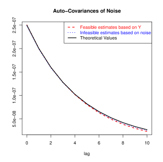
Figure 1: Comparison of estimates of auto-covariances and auto-correlations.

Figure 1 demonstrates that under Assumption (NO-1), our estimates are comparable to the infeasible estimates based on the noise process, which is the best one can hope for; both are almost indistinguishable from the theoretical values.

Next we demonstrate the central limit theorems Theorem 3.4 and Theorem 3.10. We plot the normal quantile-quantile plots of

$$\sqrt{\frac{N_{n}(T)}{\widehat{\Sigma}_{T}^{\text{\bf j},\text{\bf j},n}}}\,\Big{(}\frac{1}{N_{n}(T)}~{}U(\text{\bf j})^{n}_{T}-R(\text{\bf j})\Big{)}$$

as in (3.20) for $j=0,\cdots,8$ in Figure 2, and

$$\sqrt{\frac{N_{n}(T)}{\widehat{\mathcal{S}}(j)_{T}^{n}}}~{}(\widehat{\mbox{\rm Cor}}(j)_{n}-\mbox{\rm Cor}(j)\big{)}$$

as in (3.26) for $j=1,\cdots,9$ in Figure 3, based on 1,000 replications. All the plots support that the normality established in the theorems can be relied on in practice with sample observed at a reasonably high frequency within the time period being considered.

Figure 2: QQ-plots of estimates of auto-covariances of orders from 0 to 8, based on 1,000 replications

Figure 3: QQ-plots of estimates of auto-correlations of orders from 1 to 9, based on 1,000 replications

4.2 Under Assumption (NO-2)

The $X$ process is taken to be the same as in (4.32) above, namely, an Ornstein-Uhlenbeck process with jumps. Under Assumption (NO-2), we have an additional process $\gamma$, which we assume to be an Ornstein-Uhlenbeck process

$$d\gamma_{t}=-\rho_{\gamma}(\gamma_{t}-\mu_{\gamma})+\sigma_{\gamma}\ dW_{t},$$

where $W_{t}$ is the same Brownian motion that is used in (4.32). $\chi$ is again an AR$(1)$ process. The observations are $Y^{n}_{i}=X_{T(n,i)}+\varepsilon^{n}_{i}=X_{T(n,i)}+\gamma_{T(n,i)}\chi_{i}.$ Note that in this case the noise $\varepsilon^{n}_{i}$ is dependent on the $X$ process.

The parameters for $X$, i.e., $\rho,\mu,\sigma,\lambda,\mu^{\prime},\sigma^{\prime},\phi$ and $\chi$ are the same as in (4.33). The parameters for $\gamma$ are $\rho_{\gamma}=0.5,\mu_{\gamma}=1$ and $\sigma_{\gamma}=0.01$. We further take $\Delta_{n}=1/n:=1/93,600$.

In the estimation, we choose $k_{n}=8$ and $k_{n}^{\prime}=4$. Figure 4 compares the feasible estimates with the infeasible estimates and the theoretical values. The estimates are again based on one simulated path. More specifically, on the left panel, we use red dashed curve to report the feasible estimates of the (scaled) auto-covariances based on Theorem 3.1 ($\widehat{\mathcal{R}}(j)^{n}$ as in (3.28)); blue dotted curve to report the infeasible estimates based on the noise process $\varepsilon^{n}_{i}=\gamma_{i\Delta_{n}}\chi_{i}$ (i.e., the auto-covariance based on the simulated $\chi$ multiplied by $\widehat{\int_{0}^{1}\gamma_{s}^{2}\ ds}=\Delta_{n}\sum_{i=0}^{n}\gamma_{i\Delta_{n}}^{2}$); black solid curve to report the theoretical values, i.e., $\mathcal{R}(j)$ as in (3.27). On the right panel, we compare the feasible estimates of auto-correlations based on Theorem 3.5 ($\widehat{\mbox{\rm Cor}}(j)^{n}$ as in (3.30); see red dashed curve) with the infeasible estimates based on the noise process (auto-correlations based on the simulated $\chi$; see blue dotted curve), and the theoretical values ($\mbox{\rm Cor}(j)$ as in (4.34); see black solid curve).

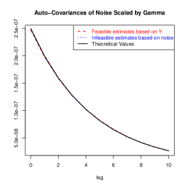
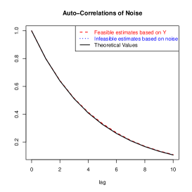
Figure 4: Comparison of estimates of auto-covariances and auto-correlations.

From Figure 4 we see again that our estimates are comparable to the infeasible estimates based on the noise process, and both are very close to the theoretical values.

Next we demonstrate the central limit theorems Theorem 3.5 and Theorem 3.11. The normal quantile to quantile plots of

$$\frac{1}{\sqrt{\Delta_{n}\,\widehat{\Sigma}_{T}^{\text{\bf j},\text{\bf j},n}}}\,\Big{(}\Delta_{n}\,U(\text{\bf j})^{n}_{T}-R(\text{\bf j})\int_{0}^{T}\gamma_{s}^{q(\text{\bf j})}\,ds\Big{)}$$

as in (3.19) for $j=0,\cdots,8$ are plotted in Figure 5 and the normal quantile to quantile plots of

$$\frac{1}{\sqrt{\Delta_{n}\,\widehat{\mathcal{S}}^{\prime}(j)_{T}^{n}}}~{}(\widehat{\mbox{\rm Cor}}^{\prime}(j)_{T}^{n}-\mbox{\rm Cor}(j)\big{)}$$

as in (3.31) for $j=1,\cdots,9$ are plotted in Figure 6, based on 1,000 replications. Again, the practical applicability of the established normality is strongly supported.

Figure 5: QQ-plots of estimates of auto-covariances of orders from 0 to 8, based on 1,000 replications

Figure 6: QQ-plots of estimates of auto-correlations of orders from 1 to 9, based on 1,000 replications

5 Empirical Studies

In this section we examine the dependence of the microstructure noise for several financial stocks, in particular, we estimate the auto-covariances and auto-correlations and test whether they are equal to zero, based on Theorems 3.4 and 3.10.

5.1 Citi Jan 2011 Data

We first analyze the tick-by-tick trade data of Citigroup Inc. (NYSE: C) in Jan 2011. The average observation frequency is about 246,000 per day ($T=1$). The observation times are irregular (not equidistant). We assume that the Assumption (NO-1) is satisfied. We estimate both the auto-covariances and auto-correlations of orders 0 to 30, using $\widehat{r}(j)_{n}$ as in (3.21) and $\widehat{\mbox{\rm Cor}}(j)_{n}$ as in (3.25)(with $k_{n}=8$), for each of the 20 trading days and plot them in Figure 7. Each curve in Figure 7 represents one day.

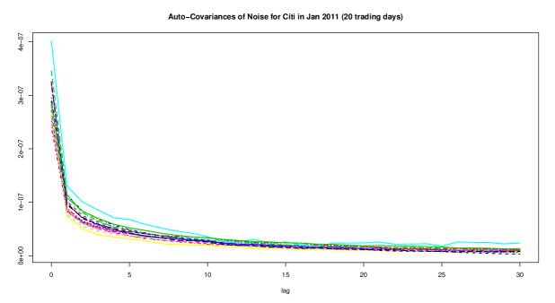
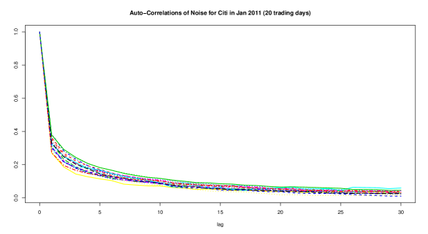
Figure 7: Estimates of auto-covariances and auto-correlations for the tick-by-tick trade data of Citigroup in Jan 2011. Each curve is for one trading day, and plots the estimates of auto-covariances (upper) or auto-correlations (lower) of orders 0 through 30.

The auto-correlations appears to decay in an exponential way, so we can assume that the mixing condition that we put in Assumption (NO-1) is satisfied. We see from the results that the noise is not un-autocorrelated; in fact, positively autocorrelated for all the days under study, at least for small lags.

Based on Theorem 3.4 we can further test whether the auto-covariances are equal to zero. More specifically, under the null hypothesis

$$H_{0}:r(j)=0,\quad\mbox{for }j\geq 1,$$

with $\text{\bf j}=(0,j)$, we have by Theorem 3.4 (and (3.20)) that

$$\sqrt{\frac{N_{n}(T)}{\widehat{\Sigma}_{T}^{\text{\bf j},\text{\bf j},n}}}\,\frac{1}{N_{n}(T)}~{}U(\text{\bf j})^{n}_{T}~{}\stackrel{{\scriptstyle\mathcal{L}}}{{\longrightarrow}}~{}\mathcal{N}(0,1).$$

So we can compute the $p$-value for testing $H_{0}:R(j)=0$ as $P\Big{(}|Z|>\sqrt{\frac{N_{n}(T)}{\widehat{\Sigma}_{T}^{\text{\bf j},\text{\bf j},n}}}\,\frac{1}{N_{n}(T)}~{}U(\text{\bf j})^{n}_{T}\Big{)}$, where $Z\sim N(0,1)$. For this dataset, we take $k_{n}=8$ and $k_{n}^{\prime}=4$ in estimating $\widehat{\Sigma}_{T}^{\text{\bf j},\text{\bf j},n}$. The $p$-values turn out to be all close to 0 (most are extremely small, the biggest one is about $0.035$), for all orders up to 30 and for all the 20 trading days under consideration. In particular, since all the estimated auto-covariances are positive, the results also imply that if one conducts a one-sided test

$$H_{0}:r(j)\leq 0,\quad\mbox{for }j\geq 1,$$

then one rejects these hypotheses at 0.05 significance level for all orders up to 30 for the data under study. We hence conclude that the auto-covariances are statistically significantly different from 0, and actually, statistically significantly bigger than 0, for all orders up to 30 and for all the 20 trading days under consideration

Based on Theorem 3.10 we can conduct tests for the auto-correlations. The results turn out to be the same as above, namely, the auto-correlations are statistically significantly different from 0, and actually, statistically significantly bigger than 0, for all orders up to 30 and for all the 20 trading days under consideration.

Theorems 3.4 and 3.10 also allow us to build confidence bands for the auto-covariances and auto-correlations. More specifically, based on Theorem 3.4 we can build 95% confidence bands for the auto-covariances $r(j)$ as

$$\left[\widehat{r}(j)\pm 1.96\cdot\sqrt{\frac{\widehat{\Sigma}_{T}^{\text{\bf j},\text{\bf j},n}}{N_{n}(T)}}\right],\quad j=0,1,2,\ldots.$$ (5.35)

And similarly Theorem 3.10 yields 95% confidence bands for the auto-correlations $\mbox{\rm Cor}(j)$ as

$$\left[\widehat{\mbox{\rm Cor}}(j)_{n}\pm 1.96\cdot\sqrt{\frac{\widehat{\mathcal{S}}(j)_{T}^{n}}{N_{n}(T)}}\right],\quad j=1,2,\ldots.$$ (5.36)

Applying these formulae to the data on January 3, 2011 we then get the confidence bands for the auto-covariances and auto-correlations of the noise, which we plot in Figure 8 below.

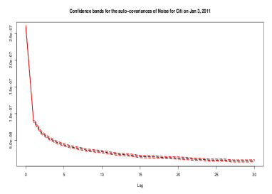
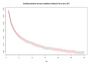
Figure 8: Confidence bands for the auto-covariances and auto-correlations for the tick-by-tick trade data of Citigroup on January 3, 2011.

We can then conclude that, for example, on January 3, 2011 the auto-correlation of the noise of any order up to 5 is greater than 0.15 or so, with 95% confidence.

5.2 Sprint-Nextel Jan 2011 Data

We next examine the tick-by-tick trade data of Sprint-Nextel Corporation (NYSE:S) in Jan 2011. The average observation frequency is about 55,000 per day ($T=1$). Assuming that the Assumption (NO-1) is satisfied, we estimate both the auto-covariances and auto-correlations of orders 0 to 30, using $\widehat{r}(j)_{n}$ as in (3.21) and $\widehat{\mbox{\rm Cor}}(j)_{n}$ as in (3.25)(with $k_{n}=8$), for each of the 20 trading days and plot them in Figure 9. Again, each curve in Figure 9 represents one day.

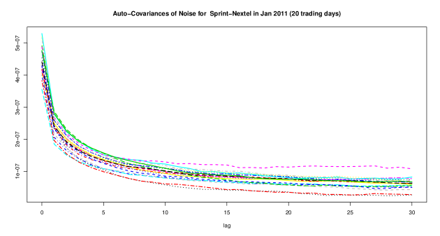
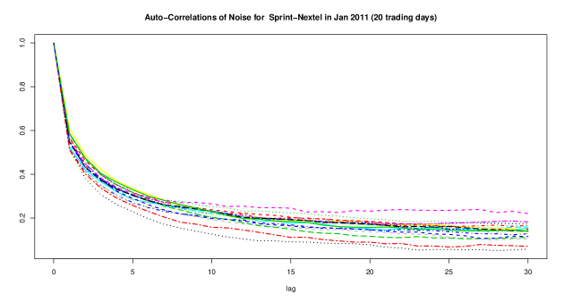
Figure 9: Estimates of auto-covariances (upper) and auto-correlations (lower) for the Sprint-Nextel trade data in Jan 2011. Each curve is for one trading day, and plots the estimates of auto-covariances or auto-correlations of orders 0 through 30.

We see similar phenomena as above, namely, (1) the auto-correlations decay fairly quickly, and (2) that the noise are not un-correlated; in fact, positively correlated for all the days under study.

One can also conduct tests as in the previous subsection. The test results are similar: for testing either the auto-covariances or auto-correlations equal zero, the $p-$values are all extremely small (all smaller than $10^{-5}$ in this case), and hence one can again conclude that the auto-covariances/auto-correlations are statistically significantly different from 0, and actually, statistically significantly bigger than 0, for all orders up to 30 and for all the 20 trading days under consideration.

We can further construct confidence bands for the auto-covariances and auto-correlations, using the formulae (5.35) and (5.36), just as in the previous subsection. The resulting bands are plotted as follows, again for the day of January 3, 2011:

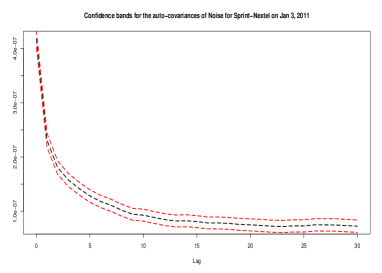
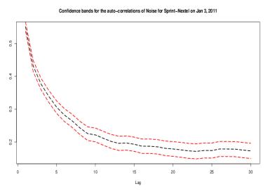
Figure 10: Confidence bands for the auto-covariances and auto-correlations for the tick-by-tick trade data of Sprint-Nextel on January 3, 2011.

Based on Figure 10 we can conclude that on January 3, 2011 the auto-correlation of the noise of any order up to 5 is greater than 0.25 or so, with 95% confidence.

6 Conclusion and discussions

In this paper we study the estimation of the (joint) moments, in particular, the auto-covariances/auto-correlations of the microstructure noise, based on high frequency data. We establish consistency as well as central-limit theorems for our proposed estimators. Simulation studies demonstrate that our estimators perform well. Empirical studies are also carried out, in which by estimation and hypothesis testing that for the stocks tested, the microstructure noises are not uncorrelated, but are actually (moderately) positively correlated.

When the noises have general auto-correlations, the existing theory based on i.i.d. noises or noises of other simple specific forms has to be modified. In Jacod et al. (2013), the authors study how the noise structure affects the estimation of volatility, and propose a volatility estimator under Assumption (NO-2). Much more has to be done to better understand the impact of the dependence structure of the market microstructure noise to further financial applications.

Appendix A Proofs

Before starting the proof we mention that, by using a classical localization procedure, for proving all the previously stated results, we can replace the three assumptions (H), (N0-1) and (NO-2) by the following stronger assumptions:

Assumption (SH) We have (H), the processes $b$ and $\sigma$ are bounded, and the stopping time $\tau_{1}$ is identically infinite (so $|\delta(\omega,t,z)|\wedge 1\leq J(z)$, where $J=J_{1}$).

Assumption (SNO-1) We have (NO-1) and $T(n,i)-T(n,i-1)\leq A\Delta_{n}$ and $\Delta_{n}N_{n}(t)\leq A_{t}$ for all $t$, for some constants $A$ and $A_{t}$.

Assumption (SNO-2) We have (NO-2) and the process $\gamma$ satisfies (SH) and is bounded.

We always assume these strengthened assumptions below, mostly without special mention. We also always assume, without mention, that $(\chi_{i})_{i\in\mathbb{Z}}$ is as in (NO-1). In all the sequel, the constant $K$ may vary from line to line, but does not depend on $n$ and on the various indices $i,j,\cdots$.

Whether the noise and the underlying process $X$ are a priori defined on the same space or not is irrelevant for the results. However, for the proofs it is convenient to suppose that $X$ and $\gamma$ are defined (and satisfy the relevant assumptions) on a space $(\Omega^{(0)},\mathcal{F}_{\infty},(\mathcal{F}_{t})_{t\geq 0},\mathbb{P}^{(0)})$, whereas the sequence $(\chi_{i})_{i\in\mathbb{Z}}$ is defined on another space $(\Omega^{(1)},\mathcal{G},(\mathcal{G}_{i})_{i\in\mathbb{Z}},\mathbb{P}^{(1)})$, with $\mathcal{G}_{i}=\sigma(\chi_{k}:j\leq i)$ and $\mathcal{G}^{i}=\sigma(\chi_{k}:j\geq i)$, and we set

$$\Omega=\Omega^{(0)}\times\Omega^{(1)},\qquad\mathcal{F}=\mathcal{F}_{\infty}\otimes\mathcal{G},\qquad\mathbb{P}=\mathbb{P}^{(0)}\otimes\mathbb{P}^{(1)}.$$

As usual, any variable or process or $\sigma$-field on $\Omega^{(j)}$ for $j=1,2$ is also considered, with the same notation, as defined on the product $\Omega$.

The space $(\Omega^{(1)},\mathcal{F}^{(1)},(\mathcal{G}_{i})_{i\in\mathbb{Z}},\mathbb{P}^{(1)})$ is naturally endowed with a measure-preserving and invertible transformation $\theta$ such that $\chi_{i+j}=\chi_{i}\!\circ\theta^{j}$ for all $i,j\in\mathbb{Z}$, and $\theta$ is ergodic by the $\rho$-mixing property. Let us also recall a consequence of the definition of the mixing coefficients $\rho_{j}$, and of the product structure of the space $(\Omega,\mathcal{F},\mathbb{P})$. We set $\mathcal{H}_{i}=\mathcal{F}_{\infty}\otimes\mathcal{G}_{i}$. If $\xi$ is a centered  square-integrable variable on $(\Omega^{(1)},\mathcal{F}^{(1)},(\mathcal{G}_{i})_{i\in\mathbb{Z}},\mathbb{P}^{(1)})$, which is measurable with respect to $\mathcal{G}^{0}=\sigma(\chi_{i}:i\geq 0)$, we have

$$\mathbb{E}\big{(}|\mathbb{E}(\xi\circ\theta^{i+j}\mid\mathcal{H}_{i})|^{2}\big{)}~{}\leq~{}\rho_{j}^{2}\,\mathbb{E}(\xi^{2})~{}\leq~{}\frac{K\,\mathbb{E}(\xi^{2})}{j^{2v}}.$$ (A.1)

This yields the following useful estimate: if $\xi$ is $\mathcal{G}_{i}$-measurable and $\xi^{\prime}$ is $\mathcal{G}^{i+j}$-measurable, both square-integrable, by (2.3) applied to $U=(\xi\circ\theta^{-i}-E(\xi))/\sqrt{\text{var}(\xi)}$ and $U^{\prime}=(\xi^{\prime}\circ\theta^{-i}-E(\xi^{\prime}))/\sqrt{\text{var}(\xi^{\prime})}$, plus $\rho_{k}(\chi)\leq K/k^{v}$ and $\mathbb{E}(U)=\mathbb{E}(U^{\prime})=0$ and by the stationarity, we have

$$\big{|}\,\mathbb{E}(\xi\,\xi^{\prime})\big{|} =\big{|}\mathbb{E}(\xi)\,\mathbb{E}(\xi^{\prime})+\mathbb{E}(\xi)\,\mathbb{E}(U^{\prime})\,\sqrt{\text{var}(\xi^{\prime})}+\mathbb{E}(\xi^{\prime})\,\mathbb{E}(U)\,\sqrt{\text{var}(\xi)}$$

$$\qquad\qquad+\mathbb{E}(UU^{\prime})\,\sqrt{\text{var}(\xi)\,\text{var}(\xi^{\prime})}\,\big{|}$$

$$\leq\big{|}\,\mathbb{E}(\xi)\,\mathbb{E}(\xi^{\prime})\big{|}+\frac{K}{j^{v}}\,\sqrt{\mathbb{E}(\xi^{2})\,\mathbb{E}(\xi^{\prime 2})}.$$ (A.2)

Finally, recall that, if $V$ is a semimartingale on $(\Omega^{(0)},\mathcal{F}^{(0)},(\mathcal{F}_{t})_{t\geq 0},\mathbb{P}^{(0)})$ which satisfies (SH), then for any finite stopping time $S$ we have for $q\geq 2$ and $t\geq 0$:

$$\big{|}\,\mathbb{E}(V_{S+t}-V_{S}\mid\mathcal{F}_{S})\big{|}\leq Kt,\qquad\mathbb{E}\Big{(}\sup_{s\in[0,t]}|V_{S+s}-V_{S}|^{q}\mid\mathcal{F}_{S}\Big{)}\leq K_{q}\,t.$$ (A.3)

A.1 Some Result about Stationary Processes.

In this subsection we consider a sequence $\xi^{n}=(\xi^{n,j})_{1\leq j\leq d}$ of $d$-dimensional variables on the space $(\Omega^{(1)},\mathcal{F}^{(1)},\mathbb{P}^{(1)})$, satisfying the following, where $w_{n}$ and $w$ are integers with $w_{n}\geq w\geq~{}0$:

$$\begin{array}[]{l}\xi^{n}~{}\stackrel{{\scriptstyle\mathbb{P}}}{{\longrightarrow}}~{}\xi,\qquad\mathbb{E}(\xi^{n})=0,\qquad\sup_{n\in\mathbb{N}}\,\mathbb{E}(\|\xi^{n}\|^{p})<\infty~{}~{}\forall\,p>0\\ \xi^{n}~{}~{}\text{is measurable with respect to the $\sigma$-field $\mathcal{G}^{0}\cap\mathcal{G}_{w_{n}}=\sigma(\chi_{i}:0\leq i\leq w_{n})$}\\ \xi~{}~{}\text{is measurable with respect to the $\sigma$-field $\mathcal{G}^{0}\cap\mathcal{G}_{w}=\sigma(\chi_{i}:0\leq i\leq w)$}.\end{array}$$ (A.4)

Note that $\mathbb{E}(\xi)=0$, whereas $w_{n}\to w$ is not assumed. We write $\xi^{n}_{i}=\xi^{n}\circ\theta^{i}$ and $\xi_{i}=\xi\circ\theta^{i}$. Then (A.1) and (A.2) yield

$$\begin{array}[]{l}\mathbb{E}\big{(}\|\mathbb{E}(\xi^{n}_{m+i}\mid\mathcal{H}_{m})\|^{2}\big{)}~{}=~{}\mathbb{E}\big{(}\|\mathbb{E}(\xi^{n}_{m+i}\mid\mathcal{G}_{m})\|^{2}\big{)}~{}\leq~{}K\mathbb{E}(\|\xi^{n}\|^{2})/i^{2v}~{}\leq~{}K/i^{2v}\\ \big{|}\,\mathbb{E}(\xi^{n,j}_{m}\,\xi^{n,k}_{m+i})\big{|}~{}\leq~{}K\mathbb{E}(\|\xi^{n}\|^{2})/((i-w_{n})\vee 1)^{v}~{}\leq~{}K/((i-w_{n})\vee 1)^{v}\end{array}$$ (A.5)

if $i\geq 1$, and the same for $\xi_{m+i}$ with $w_{n}$ replaced by $w$ in the second inequality. Since $v>1$ we deduce that the following define a covariance matrix:

$$a^{jk}=\mathbb{E}(\xi_{0}^{j}\,\xi_{0}^{k})+\sum_{i=1}^{\infty}\big{(}\mathbb{E}(\xi_{0}^{j}\,\xi_{i}^{k})+\mathbb{E}(\xi_{i}^{j}\,\xi_{0}^{k})\big{)}.$$ (A.6)

In the simple situation where $\xi^{n}=\xi$ and $w_{n}=0$ (so $\xi$ is a function of $\chi_{0}$), a trivial multi-dimensional extension of Corollary VIII.3.106 of Jacod and Shiryaev (2003) yields a Central Limit Theorem which says that

$$\frac{1}{\sqrt{u_{n}}}\,\sum_{i=1}^{[tu_{n}]}\xi_{i}~{}\stackrel{{\scriptstyle\mathcal{L}}}{{\Longrightarrow}}~{}B,$$ (A.7)

for any sequence $u_{n}\to\infty$, where

$$\text{$B$ a $d$-dimensional Brownian motion with covariance}~{}~{}\mathbb{E}(B^{j}_{1}\,B^{k}_{1})=a^{jk}.$$ (A.8)

We need to extend this result when $\xi^{n}$ depends on $n$, subject to (A.4), and $w_{n}\geq 0$; this leads us to consider the following processes, where as above $u_{n}$ is a sequence tending to $\infty$ and $u^{\prime}_{n}\geq 0$ is another sequence of integers such that $u^{\prime}_{n}/u_{n}\to 0$:

$$G^{n}=(G^{n,j})_{1\leq j\leq d},\quad\text{where}~{}~{}G^{n,j}_{t}=\frac{1}{\sqrt{u_{n}}}\,\sum_{i=0}^{[u_{n}t]-u^{\prime}_{n}}\xi_{i}^{n,j}.$$ (A.9)

This will accommodate Theorem 3.4, whereas for Theorem 3.5 we additionally have random weights. In this case the observations are equally spaced, and we need a normalization connected with the “calendar” time. So we set, with $u^{\prime}_{n}\geq 0$ a sequence of integers such that $u^{\prime}_{n}\Delta_{n}\to 0$,

$$H^{n}=(H^{n,j})_{1\leq j\leq d},\quad\text{where}~{}~{}H^{n,j}_{t}=\sqrt{\Delta_{n}}\,\sum_{i=0}^{[t/\Delta_{n}]-u^{\prime}_{n}}V^{j}_{i\Delta_{n}}\,\xi_{i}^{n,j},$$ (A.10)

where $V=(V^{j})_{1\leq j\leq d}$ is a $d$-dimensional bounded Itô semimartingale satisfying (SH) on $(\Omega^{(0)},\mathcal{F}^{(0)},(\mathcal{F}_{t}),\mathbb{P}^{(0)})$.

Theorem A.1

(a) Under (A.4) and (NO-1), and if $u_{n}\to\infty$ and $w_{n}^{2}/u_{n}\to 0$ and $u^{\prime}_{n}/u_{n}\to 0~{}$, for any $t>0$ the variables $G^{n}_{t}$ converge in law to $\mathcal{N}(0,at)$, with the matrix $a$ defined by (A.6).

(b) Under (A.4) and (NO-2), and if $w_{n}^{2}\Delta_{n}\to 0$ and $u^{\prime}_{n}\Delta_{n}\to 0$, for any $t>0$ the variables $H^{n}_{t}$ converge $\mathcal{F}_{\infty}$-stably in law to a variable $H_{t}$ defined on an extension $(\widetilde{\Omega},\widetilde{\mathcal{F}},\widetilde{\mathbb{P}})$ of the space, and which conditionally on $\mathcal{F}_{\infty}$ is centered Gaussian with (conditional) covariance

$$\widetilde{\mathbb{E}}(H^{j}_{t}\,H^{k}_{t}\mid\mathcal{F}_{\infty})~{}=~{}a^{jk}\int_{0}^{t}V^{j}_{s}\,V^{k}_{s}\,ds.$$ (A.11)

A way of realizing the limit $H$ above is to take $B$ as in (A.8) and independent of $\mathcal{F}_{\infty}$, and to put

$$H^{j}_{t}~{}=~{}\int_{0}^{t}V^{j}_{s}\,dB^{j}_{s}.$$ (A.12)

Proof. 1) We start with (b), which is more complicated than (a). By (A.5) and the Cauchy-Schwarz inequality, $\sum_{i\geq 1}\mathbb{E}(\|\mathbb{E}(\xi^{n}_{i}\mid\mathcal{H}_{m})||)<\infty$ for any $m$, whereas $V$ is bounded, so the following $d$-dimensional variables $U^{n}_{m}$ and $M^{n}_{m}$ are well defined, componentwise:

$$\begin{array}[]{l}U^{n,j}_{m}=\sqrt{\Delta_{n}}\sum_{i=(m-w_{n})^{+}}^{\infty}V^{j}_{i\Delta_{n}}\,\mathbb{E}(\xi^{n,j}_{i}\mid\mathcal{H}_{m})\\ M^{n,j}_{m}=\sqrt{\Delta_{n}}\sum_{i=0}^{\infty}V^{j}_{i\Delta_{n}}\big{(}\mathbb{E}(\xi_{i}^{n,j}\mid\mathcal{H}_{m})-\mathbb{E}(\xi_{i}^{n,j}\mid\mathcal{H}_{0})\big{)}\end{array}$$

and we write $\overline{M}{}^{n}_{m}$ for the same variables as $M^{n}_{m}$, with $\xi^{n}$ substituted with $\xi$. Since $\xi^{n}_{i}$ is $\mathcal{H}_{i+w_{n}}$-measurable, we have $\mathbb{E}(\xi_{i}^{n}\mid\mathcal{H}_{[t/\Delta_{n}]+w_{n}-u^{\prime}_{n}+1})=\xi_{i}^{n}$ when $i\leq[t/\Delta_{n}]-u^{\prime}_{n}$, hence

$$\,H^{n}_{t}=M^{n}_{[t/\Delta_{n}]+w_{n}-u^{\prime}_{n}+1}+U^{n}_{0}-U^{n}_{[t/\Delta_{n}]+w_{n}-u^{\prime}_{n}+1}.$$ (A.13)

2) In this step we prove that, for any $t>0$, we have

$$U^{n}_{[t/\Delta_{n}]+w_{n}-u^{\prime}_{n}+1}~{}\stackrel{{\scriptstyle\mathbb{P}}}{{\longrightarrow}}~{}0,\quad\mbox{and}\quad U^{n}_{0}~{}\stackrel{{\scriptstyle\mathbb{P}}}{{\longrightarrow}}~{}0.$$ (A.14)

We shall only prove the first convergence as the second can be proved similarly. To this end, we write $m_{n}=[t/\Delta_{n}]+w_{n}-u^{\prime}_{n}+1$, and since $u^{\prime}_{n}\Delta_{n}\to 0$ and $t>0$ we may assume $m_{n}>w_{n}$. Then we have $U^{n}_{m_{n}}=A_{n}+B_{n}$, where

$$A_{n}=\sqrt{\Delta_{n}}\,\sum_{i=1+m_{n}}^{\infty}V^{j}_{i\Delta_{n}}\,\mathbb{E}(\xi^{n,j}_{i}\mid\mathcal{H}_{m_{n}}),\qquad B_{n}=\sqrt{\Delta_{n}}\,\sum_{i=m_{n}-w_{n}}^{m_{n}}V^{j}_{i\Delta_{n}}\,\mathbb{E}(\xi^{n,j}_{i}\mid\mathcal{H}_{m_{n}}).$$

Since $V$ is bounded, we deduce from (A.5) and Cauchy-Schwarz inequality that

$$\mathbb{E}(\|A_{n}\|^{2})\leq K\Delta_{n}\sum_{i,j=1+m_{n}}^{\infty}\mathbb{E}\big{(}\|\mathbb{E}(\xi^{n}_{i}\mid\mathcal{H}_{m_{n}})\|\,\|\mathbb{E}(\xi^{n}_{j}\mid\mathcal{H}_{m_{n}})\|\big{)}\leq K\Delta_{n},$$

hence $A_{n}\stackrel{{\scriptstyle\mathbb{P}}}{{\longrightarrow}}0$. Next, we have $\mathbb{E}(\|\xi^{n}_{i}\|^{2})\leq K$ by (A.4), hence $\mathbb{E}(\|B_{n}\|^{2})$ is obviously smaller than $K\Delta_{n}w_{n}^{2}$ because the sum defining $B_{n}$ contains $w_{n}$ terms. Since $\Delta_{n}w_{n}^{2}\to 0$ we deduce $B_{n}\stackrel{{\scriptstyle\mathbb{P}}}{{\longrightarrow}}0$, hence the first convergence in (A.14).

3) In this step we prove

$$\|M^{n}_{[t/\Delta_{n}]+w_{n}-u^{\prime}_{n}+1}-\overline{M}{}^{n}_{[t/\Delta_{n}]+w_{n}-u^{\prime}_{n}+1}\|~{}\stackrel{{\scriptstyle\mathbb{P}}}{{\longrightarrow}}~{}0.$$ (A.15)

Setting $\xi^{\prime n}_{i}=\xi^{n}_{i}-\xi_{i}$ and again $m_{n}=[t/\Delta_{n}]+w_{n}-u^{\prime}_{n}+1$, we observe that $M^{n}_{m_{n}}-\overline{M}{}^{n}_{m_{n}}=\sum_{k=1}^{m_{n}}\eta^{n}_{k}$, where

$$\eta^{n,j}_{k}~{}=~{}\sqrt{\Delta_{n}}\,\sum_{i\geq 0}V^{j}_{i\Delta_{n}}\,\big{(}\mathbb{E}(\xi^{\prime n,j}_{i}\mid\mathcal{H}_{k})-\mathbb{E}(\xi^{\prime n,j}_{i}\mid\mathcal{H}_{k-1})\big{)}$$

is a martingale increment, relative to the discrete time filtration $(\mathcal{H}_{k})_{k\geq 0}$, hence $\mathbb{E}((M^{n,j}_{m_{n}}-\overline{M}{}^{n,j}_{m_{n}})^{2})=\sum_{k=1}^{m_{n}}\mathbb{E}((\eta^{n,j}_{k})^{2})$. By successive conditioning,

$$\begin{array}[]{l}\sum_{k=1}^{m_{n}}\mathbb{E}((\eta^{n,j}_{k})^{2})=\Delta_{n}\mathbb{E}\Big{(}\sum_{k=1}^{m_{n}}\sum_{i,l\geq 0}V^{j}_{i\Delta_{n}}\,V^{j}_{l\Delta_{n}}\,\big{(}\mathbb{E}(\xi^{\prime n,j}_{i}\mid\mathcal{H}_{k})\,\mathbb{E}(\xi^{\prime n,j}_{l}\mid\mathcal{H}_{k})\\ \hskip 199.16928pt-\mathbb{E}(\xi^{\prime n,j}_{i}\mid\mathcal{H}_{k-1})\,\mathbb{E}(\xi^{\prime n,j}_{l}\mid\mathcal{H}_{k-1})\big{)}\Big{)}\end{array}$$

and the double series $\sum_{i,l}$ inside the expectation above is absolutely convergent (almost surely). Hence we may permute the order of summation over $(i,l)$ and over $k$, and thus get $\mathbb{E}((M^{n,j}_{m_{n}}-\overline{M}{}^{n,j}_{m_{n}})^{2})=D^{n}_{m_{n}}-D^{n}_{0}$, where

$$D^{n}_{k}=\Delta_{n}\mathbb{E}\Big{(}\sum_{i,l\geq 0}V^{j}_{i\Delta_{n}}\,V^{j}_{l\Delta_{n}}\,\mathbb{E}(\xi^{\prime n,j}_{i}\mid\mathcal{H}_{k})\,\mathbb{E}(\xi^{\prime n,j}_{l}\mid\mathcal{H}_{k}\Big{)}.$$

We have $D^{n}_{k}=\sum_{r=1}^{7}D(r)^{n}_{k}$, where (with an empty sum set to $0$)

$$\begin{array}[]{l}D(1)^{n}_{k}=\Delta_{n}\mathbb{E}\Big{(}\sum_{i\geq k+1}(V^{j}_{i\Delta_{n}})^{2}\,(\mathbb{E}(\xi^{\prime n,j}_{i}\mid\mathcal{H}_{k}))^{2}\Big{)}\\ D(2)^{n}_{k}=\Delta_{n}\mathbb{E}\Big{(}\sum_{0\vee(k-w_{n})<i\leq k}(V^{j}_{i\Delta_{n}})^{2}\,(\mathbb{E}(\xi^{\prime n,j}_{i}\mid\mathcal{H}_{k}))^{2}\Big{)}\\ D(3)^{n}_{k}=\Delta_{n}\mathbb{E}\Big{(}\sum_{0\leq i\leq k-w_{n}}(V^{j}_{i\Delta_{n}})^{2}\,(\mathbb{E}(\xi^{\prime n,j}_{i}\mid\mathcal{H}_{k}))^{2}\Big{)}\\ D(4)^{n}_{k}=2\Delta_{n}\mathbb{E}\Big{(}\sum_{l>i>k}V^{j}_{i\Delta_{n}}\,V^{j}_{l\Delta_{n}}\,\mathbb{E}(\xi^{\prime n,j}_{i}\mid\mathcal{H}_{k})\,\mathbb{E}(\xi^{\prime n,j}_{l}\mid\mathcal{H}_{k})\Big{)}\\ D(5)^{n}_{k}=2\Delta_{n}\mathbb{E}\Big{(}\sum_{0\vee(k-w_{n})<i\leq k}\sum_{l>k}V^{j}_{i\Delta_{n}}\,V^{j}_{l\Delta_{n}}\,\mathbb{E}(\xi^{\prime n,j}_{i}\mid\mathcal{H}_{k})\,\mathbb{E}(\xi^{\prime n,j}_{l}\mid\mathcal{H}_{k})\Big{)}\\ D(6)^{n}_{k}=2\Delta_{n}\mathbb{E}\Big{(}\sum_{0\vee(k-w_{n})<i<l\leq k}V^{j}_{i\Delta_{n}}\,V^{j}_{l\Delta_{n}}\,\mathbb{E}(\xi^{\prime n,j}_{i}\mid\mathcal{H}_{k})\,\mathbb{E}(\xi^{\prime n,j}_{l}\mid\mathcal{H}_{k})\Big{)}\\ D(7)^{n}_{k}=2\Delta_{n}\mathbb{E}\Big{(}\sum_{0\leq i\leq k-w_{n}}\sum_{l>i}V^{j}_{i\Delta_{n}}\,V^{j}_{l\Delta_{n}}\,\mathbb{E}(\xi^{\prime n,j}_{i}\mid\mathcal{H}_{k})\,\mathbb{E}(\xi^{\prime n,j}_{l}\mid\mathcal{H}_{k})\Big{)}.\end{array}$$

Since $V$ is bounded, (A.5) applied with $\xi^{\prime n}$ and with $\alpha_{n}=\mathbb{E}(\|\xi^{n}-\xi\|^{2})$ yields $D(r)^{n}_{k}\leq K\Delta_{n}\alpha_{n}$ for $r=1,4$ (recall $v>1$). Next, one has $D(r)^{n}_{k}\leq K\Delta_{n}\alpha_{n}w_{n}$ for $r=2$ and also for $r=5$ by applying (A.5) again, whereas $D(6)^{n}_{k}\leq K\Delta_{n}\alpha_{n}w_{n}^{2}$. Finally, since $\mathbb{E}(\xi^{\prime n}_{i}\mid\mathcal{H}_{k})=\xi^{\prime n}_{i}$ when $i\leq k-w_{n}$, one has $D(3)^{n}_{k}\leq K\Delta_{n}\alpha_{n}(1+(k-w_{n})^{+})$ and one can rewrite $D(7)^{n}_{k}$ as

$$D(7)^{n}_{k}=2\Delta_{n}\mathbb{E}\Big{(}\sum_{0\leq i\leq k-w_{n}}\sum_{l>i}V^{j}_{i\Delta_{n}}\,V^{j}_{l\Delta_{n}}\,\xi^{\prime n,j}_{i}\,\mathbb{E}(\xi^{\prime n,j}_{l}\mid\mathcal{H}_{i+1})\Big{)},$$

and another application of (A.5) yield $D(7)^{n}_{k}\leq K\Delta_{n}\alpha_{n}(1+(k-w_{n})^{+})$. Putting all these estimates together (for $k=0$ and for $k=m_{n}$, and since $w_{n}\geq 1$) gives us

$$\mathbb{E}((M^{n,j}_{m_{n}}-\overline{M}{}^{n,j}_{m_{n}})^{2})\leq K\Delta_{n}\alpha_{n}\big{(}w_{n}^{2}+[t/\Delta_{n}]\big{)}.$$

We have $\alpha_{n}\to 0$ and $\Delta_{n}w_{n}^{2}\to 0$ by hypothesis, and (A.15) follows.

4) In view of (A.13), (A.14) and (A.15) it remains to prove the $\mathcal{F}_{\infty}$-stable convergence of the variables $\overline{M}{}^{n}_{[t/\Delta_{n}]+w_{n}-u^{\prime}_{n}+1}$, and we actually prove a stronger result. Namely, we will show the $\mathcal{F}_{\infty}$-stable convergence of the processes $\overline{M}{}^{n}_{[t/\Delta_{n}]}$ to a process $H$ which conditionally on $\mathcal{F}_{\infty}$ is a centered continuous Gaussian martingale with covariance given by (A.11) for any $t\geq 0$ (since $\Delta_{n}(w_{n}-u^{\prime}_{n}+1)\to 0$ this implies the convergence of $\overline{M}{}^{n}_{[t/\Delta_{n}]+w_{n}-u^{\prime}_{n}+1}$ toward $H_{t}$).

As in Step 3, $\overline{M}{}^{n}_{l}=\sum_{m=1}^{l}\zeta^{n}_{m}$, where

$$\zeta_{m}^{n,j}=\sqrt{\Delta_{n}}\,\sum_{i=0}^{\infty}V^{j}_{i\Delta_{n}}\,\beta^{j}_{i,m},\quad\beta^{j}_{i,m}=\mathbb{E}(\xi_{i}^{j}\mid\mathcal{H}_{m})-\mathbb{E}(\xi_{i}^{j}\mid\mathcal{H}_{m-1}),$$

and each $\zeta^{n}_{m}$ is a martingale increment. Hence, if

$$c_{m}^{n,jk}=\mathbb{E}(\zeta^{n,j}_{m}\,\zeta^{n,k}_{m}\mid\mathcal{H}_{m-1}),\qquad c(\varepsilon)_{m}^{n}=\mathbb{E}(\|\zeta^{n}_{m}\|^{2}\,1_{\{\|\zeta^{n}_{m}\|>\varepsilon\}}\mid\mathcal{H}_{m-1}),$$

we deduce from Theorems VIII.3.22 and VIII.5.14 of Jacod and Shiryaev (2003) the $\mathcal{F}_{\infty}$-stable convergence of the processes $\overline{M}{}^{n}_{[t/\Delta_{n}]}$ to $H$, as soon as we have the following two properties, for all $t,\varepsilon>0$:

$$\sum_{m=1}^{[t/\Delta_{n}]}c_{m}^{n,jk}~{}\stackrel{{\scriptstyle\mathbb{P}}}{{\longrightarrow}}~{}a^{jk}\int_{0}^{t}V^{j}_{s}\,V^{k}_{s}\,ds\,,\qquad\sum_{m=1}^{[t/\Delta_{n}]}c(\varepsilon)_{m}^{n}~{}\stackrel{{\scriptstyle\mathbb{P}}}{{\longrightarrow}}~{}0.$$ (A.16)

The second one is easy to prove. Indeed, if $\widetilde{\beta}_{m}=\sum_{i\in\mathbb{Z}}\|\beta_{i,m}\|$, we have $\|\zeta^{n}_{m}\|\leq A\sqrt{\Delta_{n}}\,\widetilde{\beta}_{m}$ for some $A>0$: we allow the index $i$ to be negative, so that we can apply the obvious relation $\beta_{i,m}=\beta_{i-m,0}\circ\theta^{m}$ (for all $i,m\in\mathbb{Z}$) to obtain $\widetilde{\beta}_{m}=\widetilde{\beta}_{0}\circ\theta^{m}$. A priori $\widetilde{\beta}_{m}$ could be infinite, however $\beta_{i,m}=0$ when $i<m-w$ by (A.4), so (A.5) for $\xi$ implies that $\mathbb{E}((\widetilde{\beta}_{m})^{2})\leq K$. Then by stationarity

$$\begin{array}[]{c}\mathbb{E}(c(\varepsilon)^{n}_{m})\leq A^{2}\Delta_{n}\mathbb{E}\big{(}\widetilde{\beta}_{m}^{2}\,1_{\{\widetilde{\beta}_{m}>\varepsilon/(A\sqrt{\Delta_{n}})\}}\big{)}=A^{2}\Delta_{n}\overline{\alpha}{}(\varepsilon)_{n}\\ \text{where}~{}~{}\overline{\alpha}{}(\varepsilon)_{n}=\mathbb{E}\big{(}(\widetilde{\beta}_{0})^{2}\,1_{\{\widetilde{\beta}_{0}>\varepsilon/(A\sqrt{\Delta_{n}})\}}\big{)}.\end{array}$$

Now, $\overline{\alpha}{}(\varepsilon)_{n}\to 0$ because $\mathbb{E}(\widetilde{\beta}_{0}^{2})\leq K$, and the second part of (A.16) follows.

5) By virtue of the square-integrability of $\widetilde{\beta}_{m}$, the $d$-dimensional variables $\overline{\beta}{}_{m}=\sum_{i\geq 0}\beta_{i,m}$ are well-defined, square-integrable, and also $\overline{\beta}{}_{m}=\overline{\beta}{}_{w+1}\circ\theta^{m-w-1}$ for all $m\geq w+1$ (this is wrong when $1\leq m\leq w$). In this step, we show that

$$|\mathbb{E}(\overline{\beta}{}_{m}^{j}\,\overline{\beta}{}_{m}^{k})|\leq K,\qquad\mbox{and if }~{}m\geq w+1,\mbox{ then }~{}\mathbb{E}(\overline{\beta}{}_{m}^{j}\,\overline{\beta}{}_{m}^{k})=a^{jk},$$ (A.17)

with $a^{jk}$ given by (A.6). The first estimate follows from $\|\overline{\beta}{}_{m}\|\leq\widetilde{\beta}_{m}=\widetilde{\beta}_{0}\circ\theta^{m}$ and $\widetilde{\beta}_{0}\in\mathbb{L}^{2}$. For the second property, by polarization it is enough to show it in the one-dimensional case $d=1$, and so below we omit $j,k$. The variable $\beta_{i,m}=\mathbb{E}(\xi_{i}\mid\mathcal{H}_{m})-\mathbb{E}(\xi_{i}\mid\mathcal{H}_{m-1})$ is $\mathcal{H}_{m}$-measurable with vanishing $\mathcal{H}_{m-1}$-conditional mean, whereas $\xi_{i+1}\,\mathbb{E}(\xi_{l+1}\mid\mathcal{H}_{m})=\big{(}\xi_{i}\,\mathbb{E}(\xi_{l}\mid\mathcal{H}_{m-1})\big{)}\circ\theta$. Then

$$\mathbb{E}(\beta_{i,m}\,\beta_{l,m})=\mathbb{E}(\xi_{i}\,\beta_{l,m})=\mathbb{E}\big{(}\mathbb{E}(\xi_{i}-\xi_{i+1}\mid\mathcal{H}_{m})\,\mathbb{E}(\xi_{l}\mid\mathcal{H}_{m})\big{)}+\mathbb{E}\big{(}\mathbb{E}(\xi_{i+1}\mid\mathcal{H}_{m})\,\mathbb{E}(\xi_{l}-\xi_{l+1}\mid\mathcal{H}_{m})\big{)},$$

hence for any $L>2m$:

$$\sum_{i,l=0}^{L}\mathbb{E}(\beta_{i,m}\,\beta_{l,m})=\sum_{l=0}^{L}\mathbb{E}\big{(}\mathbb{E}(\xi_{0}\mid\mathcal{H}_{m})\,\mathbb{E}(\xi_{l}+\xi_{l+1}\mid\mathcal{H}_{m})\big{)}-\sum_{l=0}^{L}\mathbb{E}\big{(}\mathbb{E}(\xi_{L+1}\mid\mathcal{H}_{m})\,\mathbb{E}(\xi_{l}+\xi_{l+1}\mid\mathcal{H}_{m})\big{)}.$$

By (A.5) the $l$th summand in the last sum above is smaller in absolute value than $K/L^{v}$ always, and than $K/L^{v}l^{v}$ when $l>2m$. Since $v>1$, by letting $L\to\infty$ we obtain that

$$\mathbb{E}((\overline{\beta}{}_{m})^{2})=\sum_{l=0}^{\infty}\mathbb{E}\big{(}\mathbb{E}(\xi_{0}\mid\mathcal{H}_{m})\,\mathbb{E}(\xi_{l}+\xi_{l+1}\mid\mathcal{H}_{m})\big{)}=\mathbb{E}(\xi_{0}^{2})+2\sum_{l=1}^{\infty}\mathbb{E}\big{(}\xi_{0}\,\xi_{l}\big{)},$$

the last equality following from the fact that $m\geq w+1$, hence $\xi_{0}$ is $\mathcal{H}_{m}$-measurable. The right side above is (A.6) in the one-dimensional case, and thus the last part of (A.17) holds.

6) In this step we set $c^{\prime jk}_{m}=\mathbb{E}\big{(}\overline{\beta}{}^{j}_{m}\,\overline{\beta}{}^{k}_{m}\mid\mathcal{H}_{m-1}\big{)}$ and prove that

$$\sum_{m=1}^{[t/\Delta_{n}]}\big{(}c_{m}^{n,jk}-\Delta_{n}\,V_{(m-1)\Delta_{n}}^{j}\,V_{(m-1)\Delta_{n}}^{k}\,c^{\prime jk}_{m}\big{)}~{}\stackrel{{\scriptstyle\mbox{\tiny u.c.p.}}}{{\Longrightarrow}}~{}0.$$ (A.18)

Letting $\eta^{n}_{m}$ be the $m$th summand above, we see that $\eta^{n}_{m}=\Delta_{n}\sum_{i,l\geq 0}\eta(i,l)^{n}_{m}$, where

$$\eta(i,l)^{n}_{m}=\big{(}V^{j}_{i\Delta_{n}}\,V^{k}_{l\Delta_{n}}-V^{j}_{(m-1)\Delta_{n}}\,V^{k}_{(m-1)\Delta_{n}}\big{)}\,\mathbb{E}\big{(}\beta_{i,m}^{j}\,\beta_{l,m}^{k}\mid\mathcal{H}_{m-1}\big{)}.$$

As seen before, $\beta_{i,m}=0$ when $i<m-w$ and $\mathbb{E}(\|\beta_{i,m}\|^{2})$ is smaller than $K$ always, and than $K/(i-m)^{2v}$ when $i>m$; hence by (A.3) and (A.5) we obtain if $i\leq l$

$$\mathbb{E}(|\eta(i,l)^{n}_{m}|)\leq\left\{\begin{array}[]{ll}0&\text{if}~{}~{}i<m-w\\ K\frac{1\wedge\sqrt{\Delta_{n}((l-m)\vee|m-1-i|)}}{(l-m)^{v}}&\text{if}~{}~{}m-w\leq i\leq m<l\\ K\frac{1\wedge\sqrt{\Delta_{n}(l-m)}}{(i-m)^{v}(l-m)^{v}}&\text{if}~{}~{}i>m\\ K\sqrt{\Delta_{n}}&\text{if}~{}~{}m-w\leq i\leq l\leq m,\end{array}\right.$$

and similar estimates hold when $l\leq i$. Since one can always assume $v\in(1,3/2)$, in which case $\sum_{i\geq 1}(1\wedge\sqrt{i\Delta_{n}}\,)/i^{v}\leq K\Delta_{n}^{v-1}$, we get $\mathbb{E}(|\eta^{n}_{m}|)\leq K\Delta_{n}^{v}$, and (A.18) follows.

7) By the previous step, in order to get the first part of (A.16) we are left to show

$$\Delta_{n}\sum_{m=1}^{[t/\Delta_{n}]}V_{(m-1)\Delta_{n}}^{j}\,V_{(m-1)\Delta_{n}}^{k}\,c_{m}^{\prime jk}~{}\stackrel{{\scriptstyle\mathbb{P}}}{{\longrightarrow}}~{}a^{jk}\int_{0}^{t}V^{j}_{s}\,V^{k}_{s}\,ds.$$ (A.19)

The left side above can be considered as the integral of the càdlàg function $s\mapsto V^{j}_{s}\,V^{k}_{s}$ with respect to the (random) measure $F^{n,jk}_{t}(ds)=\Delta_{n}\sum_{m=1}^{[t/\Delta_{n}]}c^{\prime jk}_{m}\textbf{\,}\delta_{(m-1)\Delta_{n}}(ds)$, where $\delta_{x}$ stands for the delta measure at $x$, so it is enough to show that $F^{n,jk}_{t}$ converges in probability to the measure $a^{jk}\,1_{[0,t]}(s)\,ds$. To this aim, it is is enough to show that

$$s\leq t~{}~{}\Rightarrow~{}~{}G^{n}_{s}~{}:=~{}\Delta_{n}\sum_{m=1}^{[s/\Delta_{n}]}c^{\prime jk}_{m}~{}\stackrel{{\scriptstyle\mathbb{P}}}{{\longrightarrow}}~{}a^{jk}\,s$$ (A.20)

(this is obvious when $k=j$, because then $F^{n,jk}_{t}$ is a positive measure; when $k\neq j$ it may be a signed measure, but with an absolute value dominated by $\frac{1}{2}\,(F^{n,jj}_{t}+F^{n,kk}_{t})$, so again (A.20) is enough).

We recall that $\overline{\beta}{}_{m}=\overline{\beta}{}_{w+1}\circ\theta^{m-w-1}$ when $m>w$, implying $c^{\prime}_{m}=c^{\prime}_{w+1}\circ\theta^{m-w+1}$, whereas it is obviously enough to show the convergence (A.20) when the sum starts at $m=w+1$. Then, the ergodic theorem and (A.17) tell us that $G^{n}_{s}$ converges a.s. (locally uniformly in $s$) to $a^{jk}s$. This completes the proof of (b).

8) Now we turn to (a). This is basically the same as (b), with the processes $V^{j}$ being identically equal to $1$, and with the convention $\Delta_{n}=1/u_{n}$ (indeed, in this case, the calendar time and the observation times $T(n,i)$ play no role at all, and neither does $\mathcal{F}_{\infty}$; so (2.4) is irrelevant, and we can set $\Delta_{n}=1/u_{n}$). So all Steps 1–7 can be reproduced, except Step 6 which is irrelevant, whereas in Step 7 we can proceed directly to (A.20).$\hfill\Box$

We will also need bounds for the moments of the processes $G^{n}$ and $H^{n}$:

Lemma A.2

Under (A.4) and if $V$ is bounded, we have

$$\begin{array}[]{lll}\text{\rm(NO-1)}&\Rightarrow&\mathbb{E}(\|G^{n}_{t}\|^{2})~{}\leq~{}K(1+w_{n})t\\ \text{\rm(NO-2)}&\Rightarrow&\mathbb{E}(\|H^{n}_{t}\|^{2})~{}\leq~{}K(1+w_{n})t.\end{array}$$

Proof. Upon setting $V^{j}_{t}=1$ and $u_{n}=1/\Delta_{n}$, the case (NO-1) reduces to the case (NO-2). By singling out each component $H^{n,j}$ we can assume $d=1$. Then we have $\mathbb{E}(|H^{n}_{t}|^{2})=\phi_{n}(t)+\psi_{n}(t)$, where

$$\begin{array}[]{l}\phi_{n}(t)=\Delta_{n}\sum_{i=0}^{[t/\Delta_{n}]-u^{\prime}_{n}}\mathbb{E}\big{(}|V_{i\Delta_{n}}|^{2}\,|\xi^{n}_{i}|^{2}\big{)}+2\Delta_{n}\sum_{0\leq i<l\leq(i+w_{n})\wedge([t/\Delta_{n}]-u^{\prime}_{n})}\mathbb{E}\big{(}V_{i\Delta_{n}}\,\xi^{n}_{i}\,V_{l\Delta_{n}}\,\xi^{n}_{l}\big{)}\\ \psi_{n}(t)=2\Delta_{n}\sum_{0\leq i<i+w_{n}<l\leq[t/\Delta_{n}]-u^{\prime}_{n}}\mathbb{E}\big{(}V_{i\Delta_{n}}\,\xi^{n}_{i}\,V_{l\Delta_{n}}\,\xi^{n}_{l}\big{)}.\end{array}$$

On the one hand, since $V$ is bounded and (A.4) holds, $|\phi_{n}(t)|\leq K(1+w_{n})t$ follows from the Cauchy-Schwarz inequality. On the other hand, $\xi^{n}_{i}$ is $\mathcal{G}_{i+w_{n}}$-measurable, so by conditioning first with respect to $\mathcal{F}_{\infty}$ we deduce from (A.5) that $\big{|}\mathbb{E}\big{(}V_{i\Delta_{n}}\,\xi^{n}_{i}\,V_{l\Delta_{n}}\,\xi^{n}_{l})\big{|}\leq K/(l-i-w_{n})^{v}$ when $l>i+w_{n}$. Since $v>1$ one deduces $\psi_{n}(t)\leq Kt$, and the result follows.$\hfill\Box$

Finally, we need to consider processes that are slightly more general than $H^{n}$, at least in the one-dimensional case. Namely, we assume (A.4) with $d=1$, and we are also given another set $(\xi^{\prime n},w^{\prime}_{n})$ satisfying (A.4) as well (we do not need a limit $\xi^{\prime}$ here), plus an arbitrary sequence of integers $\rho_{n}\geq 1$. With the same auxiliary bounded process $V$ and sequence of integers $u^{\prime}_{n}$ as above, we set

$$\overline{H}{}^{n}_{t}=\sqrt{\Delta_{n}}\,\sum_{i=0}^{[t/\Delta_{n}]-u^{\prime}_{n}}V_{i\Delta_{n}}\,\xi^{n}_{i}\,\xi^{\prime n}_{i+w_{n}+\rho_{n}}.$$ (A.21)

Lemma A.3

In the above setting, and under (NO-2), we have

$$\mathbb{E}(|\overline{H}{}^{n}_{t}|^{2})~{}\leq~{}K\Big{(}1+w_{n}^{\prime}+\frac{w_{n}}{\rho_{n}^{v}}+\frac{t}{\Delta_{n}\,\rho_{n}^{2v}}\Big{)}t.$$

Proof. Set $\xi^{\prime\prime n}_{i}=\xi^{n}_{i}\,\xi^{\prime n}_{i+w_{n}+\rho_{n}}$. By (A.4) and (A.2) applied repeatedly, we check that for $l\geq 0$,

$$\big{|}\,\mathbb{E}(\xi^{\prime\prime n}_{i}\,\xi^{\prime\prime n}_{i+l}\mid\mathcal{F}_{\infty})\big{|}\leq\left\{\begin{array}[]{ll}K&\text{if}~{}l\leq w^{\prime}_{n}\\ K/(l-w^{\prime}_{n})^{v}&\text{if}~{}w^{\prime}_{n}<l\leq w^{\prime}_{n}+\rho_{n}\\ K/\rho_{n}^{v}&\text{if}~{}w^{\prime}_{n}+\rho_{n}<l\leq w^{\prime}_{n}+\rho_{n}+w_{n}\\ K(1/\rho_{n}^{2v}+1/(l-w^{\prime}_{n}-w_{n}-\rho_{n})^{v})&\text{if}~{}l>w^{\prime}_{n}+\rho_{n}+w_{n}.\end{array}\right.$$

Since $V$ is bounded, we have

$$\mathbb{E}(|\overline{H}{}^{n}_{t}|^{2})\leq K\Delta_{n}\sum_{i=0}^{[t/\Delta_{n}]}~{}\sum_{l=0}^{[t/\Delta_{n}]}\mathbb{E}\big{(}\big{|}\,\mathbb{E}(\xi^{\prime\prime n}_{i}\,\xi^{\prime\prime n}_{i+l}\mid\mathcal{F}_{\infty})\big{|}\big{)}.$$

Then by splitting the sum over $l$ according to the four cases described above, we obtain the result.$\hfill\Box$

A.2 Further Auxiliary Results

In this subsection we gather a few results of a technical character, to be used at several places.

1) The first of these results is about asymptotically negligible triangular arrays. The setting is as follows: for each $n$ we have a discrete-time filtration $(\widetilde{\mathcal{H}}^{n}_{i})_{i\geq 0}$, an integer $w_{n}\geq 1$ (typically, $w_{n}\to\infty$), and a sequence $(\delta^{n}_{i})_{i\geq 1}$ of random variables.

Lemma A.4

In the above setting, and if further each $\delta^{n}_{i}$ is $\widetilde{\mathcal{H}}^{n}_{i+w_{n}}$-measurable, we have

$$\begin{array}[]{c}\mathbb{E}\Big{(}\sup_{s\leq t}\,\big{|}\sum_{i=1}^{[s/\Delta_{n}]}\delta^{n}_{i}\big{|}\Big{)}~{}\leq~{}K\Big{(}\frac{a_{n}t}{\Delta_{n}}+2\,\frac{\sqrt{a^{\prime}_{n}\,t\,w_{n}}}{\sqrt{\Delta_{n}}}\Big{)}\\ \text{\rm where}~{}~{}\quad a_{n}=\sup_{i\geq 1}\,\mathbb{E}\big{(}\big{|}\,\mathbb{E}(\delta^{n}_{i}\mid\widetilde{\mathcal{H}}^{n}_{i})\big{|}\big{)},\qquad a^{\prime}_{n}=\sup_{i\geq 1}\,\mathbb{E}(|\delta^{n}_{i}|^{2}).\end{array}$$ (A.22)

Proof. When $w_{n}=0$ we have $a_{n}=\sup_{i\geq 1}\,\mathbb{E}(|\delta^{n}_{i}|)$ and the result is obvious. When $w_{n}\geq 1$ we let $\delta^{\prime n}_{i}=\mathbb{E}(\delta^{n}_{i}\mid\widetilde{\mathcal{H}}^{n}_{i})$ and $\delta^{\prime\prime n}_{i}=\delta^{n}_{i}-\delta^{\prime n}_{i}$ and, for $j=1,\cdots,w_{n}$,

$$A(j)^{n}_{t}=\sum_{i=0}^{[(t-j\Delta_{n})/(w_{n}\Delta_{n})]}\delta^{\prime\prime n}_{j+iw_{n}}.$$

The summands above are martingale increments, relative to the filtration $(\widetilde{\mathcal{H}}^{n}_{j+iw_{n}})_{i\geq 0}$, hence by Doob’s inequality

$$\mathbb{E}\Big{(}\sup_{s\leq t}\,|A(j)^{n}_{s}|^{2}\Big{)}~{}\leq~{}\frac{4t\,a^{\prime}_{n}}{w_{n}\Delta_{n}}.$$

Observing that $A^{n}_{t}=\sum_{i=1}^{[t/\Delta_{n}]}\delta^{n}_{i}$ satisfies that $A_{t}^{n}=\sum_{i=1}^{[t/\Delta_{n}]}\delta^{\prime n}_{i}+\sum_{j=1}^{w_{n}}A(j)^{n}_{t}$, we deduce that

$$\mathbb{E}\Big{(}\sup_{s\leq t}\,|A^{n}_{s}|\Big{)}~{}\leq~{}\sum_{i=1}^{[t/\Delta_{n}]}\mathbb{E}\big{(}|\delta^{\prime n}_{i}|\big{)}+\sum_{j=1}^{w_{n}}\,\mathbb{E}\Big{(}\sup_{s\leq t}\,|A(j)^{n}_{s}|\Big{)},$$

and the result readily follows.$\hfill\Box$

2) Our second auxiliary result mainly compares $R(k_{n},\text{\bf j})$ defined in (3.14) with $R(\text{\bf j})$ in (3.2).

Lemma A.5

If $\text{\bf j}\in\mathcal{J}$ we have $|R(k_{n};\text{\bf j})-R(\text{\bf j})|\leq K/k_{n}^{v}$ (for a constant $K$ depending on j), hence in particular $R(k_{n};\text{\bf j})\to R(\text{\bf j})$, as $n\to\infty$. We also have $\overline{\chi}{}^{n}_{u_{n}}\stackrel{{\scriptstyle\mathbb{P}}}{{\longrightarrow}}0$ for any sequence $u_{n}$ of integers.

Proof. Letting $\text{\bf j}=(j_{1},\cdots,j_{q})\in\mathcal{J}$ and $\mu=\mu(\text{\bf j})$, and denoting by $\mathcal{Q}$ the set of all non-empty subsets $Q$ of $\{1,\cdots,q\}$, the complement of $Q$ being denoted as $Q^{c}$. (3.2) and (3.14) yield

$$R(k_{n};\text{\bf j})-R(\text{\bf j})~{}=~{}\sum_{Q\in\mathcal{Q}}(-1)^{|Q|}\phi_{n}(Q),\quad\text{where}~{}~{}\phi_{n}(Q)=\mathbb{E}\Big{(}\prod_{r\in Q^{c}}\chi_{j_{r}}~{}\prod_{r\in Q}\overline{\chi}{}^{n}_{\mu+(2r-1)k_{n}}\Big{)},$$

where $|Q|$ denotes the cardinal of $Q$. We fix $Q\in\mathcal{Q}$ and let $r_{0}=\max Q$ and $Q^{\prime}=Q\backslash\{r_{0}\}$. Then

$$\phi_{n}(Q)=\mathbb{E}\big{(}\Phi_{n}(Q)\,\overline{\chi}{}^{n}_{\mu+(2r_{0}-1)k_{n}}\big{)},\quad\text{where}~{}~{}\Phi_{n}(Q)=\prod_{r\in Q^{c}}\chi_{j_{r}}~{}\prod_{r\in Q^{\prime}}\overline{\chi}{}^{n}_{\mu+(2r-1)k_{n}}.$$

The variable $\Phi_{n}(Q)$ is $\mathcal{G}_{\mu+2(r_{0}-1)k_{n}}$-measurable, with $\mathbb{E}(\Phi_{n}(Q)^{2})\leq K$, so by the Cauchy-Schwarz inequality

$$|\phi_{n}(Q)|~{}\leq~{}K\sqrt{\mathbb{E}\big{(}\big{|}\mathbb{E}(\overline{\chi}{}^{n}_{\mu+(2r_{0}-1)k_{n}}\mid\mathcal{G}_{\mu+(2r_{0}-2)k_{n}})\big{|}^{2}\big{)}}.$$

Since $\overline{\chi}{}^{n}_{\mu+2(r_{0}-1)k_{n}}$ is $\mathcal{G}^{\mu+(2r_{0}-1)k_{n}}$-measurable, centered, and with a second moment bounded in $n$, it follows from (A.1) that $|\phi_{n}(Q)|\leq K/k_{n}^{v}$. Summing up over all $Q\in\mathcal{Q}$, we deduce the first claim.

Finally, we observe that $\mathbb{E}((\overline{\chi}{}^{n}_{u_{n}})^{2})$ is independent of $u_{n}$ and equal to $\frac{1}{k^{2}_{n}}\sum_{0\leq i,j<k_{n}}r(i-j)$, which in turn is smaller than $\frac{1}{k_{n}}\sum_{m\in\mathbb{Z}}|r(m)|<K/k_{n}$, and the last claim follows.$\hfill\Box$

3) For our last auxiliary result we suppose (SNO-2) and consider $\text{\bf j}=(j_{1},\cdots,j_{q})$ and $\text{\bf j}^{\prime}=(j^{\prime}_{1},\cdots,j^{\prime}_{q^{\prime}})$ in $\mathcal{J}$, and set $\mu=\mu(\text{\bf j})$, $\mu^{\prime}=\mu(\text{\bf j}^{\prime})$, $\mu^{\prime\prime}=\mu+\mu^{\prime}$ and $q^{\prime\prime}=q+q^{\prime}$, and also $\alpha_{n}(t)=N_{n}(t)+1-\mu-2qk_{n}$ and $\alpha^{\prime}_{n}(t)=N_{n}(t)+1-\mu^{\prime\prime}-(2q^{\prime\prime}+1)k_{n}$. The following processes are the same as $U(\text{\bf j})^{n}$ and $\overline{U}{}(\text{\bf j},\text{\bf j}^{\prime})^{n}$, when there is only noise and the process $\gamma$ is properly “frozen”:

$$\hskip-5.69054pt\begin{array}[]{l}\mathcal{U}(\text{\bf j})^{n}_{t}=\sum\limits_{i=0}^{\alpha_{n}(t)}\gamma_{i\Delta_{n}}^{q}\,\prod\limits_{r=1}^{q}(\chi_{i+j_{r}}-\overline{\chi}{}^{n}_{i+\mu+(2r-1)k_{n}})\\ \overline{\mathcal{U}}{}(\text{\bf j},\text{\bf j}^{\prime})^{n}_{t}=\sum\limits_{i=0}^{\alpha^{\prime}_{n}(t)}\gamma_{i\Delta_{n}}^{q+q^{\prime}}\,\prod\limits_{r=1}^{q}(\chi_{i+j_{r}}-\overline{\chi}{}^{n}_{i+\mu+(2r-1)k_{n}})\prod\limits_{r=1}^{q^{\prime}}(\chi_{i+\mu+(2q+1)k_{n}+j^{\prime}_{r}}-\overline{\chi}{}^{n}_{i+\mu^{\prime\prime}+(2r+2q)k_{n}})\end{array}$$ (A.23)

Lemma A.6

Under (SH) and (SNO-2) we have

$$\left.\begin{array}[]{l}\mathbb{E}\Big{(}\sup_{s\leq t}|U(\text{\bf j})^{n}_{s}-\mathcal{U}(\text{\bf j})^{n}_{s}|\Big{)}\\ \mathbb{E}\Big{(}\sup_{s\leq t}|\overline{U}{}(\text{\bf j},\text{\bf j}^{\prime})^{n}_{s}-\overline{\mathcal{U}}{}(\text{\bf j},\text{\bf j}^{\prime})_{s}^{n}|\Big{)}\end{array}\right\}\leq K_{p}(t+\sqrt{t})\big{(}k_{n}+\mu^{\prime\prime}+(k_{n}+\mu^{\prime\prime})^{1/p}\Delta_{n}^{1/p-1}\big{)}$$ (A.24)

for any $p>1$, where $K_{p}$ depends on $p$, and on $\text{\bf j},\text{\bf j}^{\prime}$ through $q,q^{\prime}$ only.

Proof. Since $U(\text{\bf j})^{n}=\overline{U}{}(\text{\bf j},\emptyset)^{n}$ and $\mathcal{U}(\text{\bf j})^{n}=\overline{\mathcal{U}}{}(\text{\bf j},\emptyset)^{n}$ (with the convention that an empty product is equal to $1$, in (A.23) for example), only the second claim needs to be proved.

1) The first step is devoted to some estimates. Set for $u,l,w\in\mathbb{N}$:

$$\begin{array}[]{ll}\zeta(1;u,l)^{n}_{i}=X_{(i+u)\Delta_{n}}-\overline{X}{}^{n}_{i+l},&\zeta(2;u,l)^{n}_{i}=(\gamma_{(i+u)\Delta_{n}}-\gamma_{i\Delta_{n}})\chi_{i+u}\\ \zeta(3;u,l)^{n}_{i}=-\frac{1}{k_{n}}\sum_{m=0}^{k_{n}-1}(\gamma_{(i+l+m)\Delta_{n}}-\gamma_{i\Delta_{n}})\chi_{i+l+m},&\zeta(4;u,l)^{n}_{i}=\gamma_{i\Delta_{n}}\,\big{(}\chi_{i+u}-\overline{\chi}{}^{n}_{i+l}\big{)}\end{array}$$

(note that $\zeta(2;u,l)^{n}_{i}$ does not depend on $l$ and $\zeta(3;u,l)^{n}_{i}$ does not depend on $u$). Upon using the second part of (A.3) with $V=X$ or with $V=\gamma$, plus the independence of $\mathcal{F}_{\infty}$ and $\mathcal{G}$ and the fact that $\chi_{i}$ has moments of all orders, plus Hölder’s inequality, we get for any $p\geq 2$:

$$\begin{array}[]{ll}\mathbb{E}\big{(}|\zeta(1;u,l)^{n}_{i}|^{p}\mid\mathcal{F}_{i\Delta_{n}}\big{)}\leq K_{p}\,\Delta_{n}(u+l+k_{n}),&\mathbb{E}\big{(}|\zeta(2;u,l)^{n}_{i}|^{p}\mid\mathcal{F}_{i\Delta_{n}}\big{)}\leq K_{p}\,\Delta_{n}\,u\\ \mathbb{E}\big{(}|\zeta(3;u,l)^{n}_{i}|^{p}\mid\mathcal{F}_{i\Delta_{n}}\big{)}\leq K_{p}\,\Delta_{n}(l+k_{n}),&\mathbb{E}\big{(}|\zeta(4;u,l)^{n}_{i}|^{p}\mid\mathcal{F}_{i\Delta_{n}}\big{)}\leq K_{p}.\end{array}$$ (A.25)

One also has the following:

$$j=1,2,3~{}~{}\Rightarrow~{}~{}\mathbb{E}\Big{(}\big{|}\,\mathbb{E}(\zeta(j;u,l)^{n}_{i}\mid\mathcal{F}_{i\Delta_{n}}\otimes\mathcal{G})\big{|}^{2}\Big{)}\leq K\Delta_{n}^{2}(u+l+k_{n})^{2},$$ (A.26)

which we prove for $j=3$ only, the cases $j=1,2$ being similar (and even simpler). Indeed, (A.3) again and the independence of $\mathcal{F}_{\infty}$ and $\mathcal{G}$ yield

$$\big{|}\,\mathbb{E}(\zeta(3;u,l)^{n}_{i}\mid\mathcal{F}_{i\Delta_{n}}\otimes\mathcal{G})\big{|}\leq\frac{K\Delta_{n}(l+k_{n})}{k_{n}}\,\sum_{m=0}^{k_{n}-1}|\chi_{i+l+m}|.$$

The moments of $\chi$ being finite, one deduces the second part of (A.26).

2) By definition, $\overline{U}{}(\text{\bf j},\text{\bf j}^{\prime})^{n}_{t}-\overline{\mathcal{U}}{}(\text{\bf j},\text{\bf j}^{\prime})^{n}_{t}=\sum_{i=0}^{\alpha^{\prime}_{n}(t)}\xi^{n}_{i}$, where

$$\begin{array}[]{lll}\xi^{n}_{i}&=&\prod\limits_{r=1}^{q}(Y^{n}_{i+j_{r}}-\overline{Y}{}^{n}_{i+\mu+(2r-1)k_{n}})\prod\limits_{r=1}^{q^{\prime}}(Y^{n}_{i+\mu+(2q+1)k_{n}+j^{\prime}_{r}}-\overline{Y}{}^{n}_{i+\mu^{\prime\prime}+(2r+2q)k_{n}})\\ &&-\gamma_{i\Delta_{n}}^{q+q^{\prime}}\,\prod\limits_{r=1}^{q}(\chi_{i+j_{r}}-\overline{\chi}{}^{n}_{i+\mu+(2r-1)k_{n}})\prod\limits_{r=1}^{q^{\prime}}(\chi_{i+\mu+(2q+1)k_{n}+j^{\prime}_{r}}-\overline{\chi}{}^{n}_{i+\mu^{\prime\prime}+(2r+2q)k_{n}}).\end{array}$$

We will rewrite this in a more convenient way. If

$$\begin{array}[]{llll}1\leq r\leq q&\Rightarrow&u_{r}^{n}=j_{r},&l^{n}_{r}=\mu+(2r-1)k_{n}\\ q<r\leq q^{\prime\prime}&\Rightarrow&u_{r}^{n}=\mu+(2q+1)k_{n}+j^{\prime}_{r-q},&l^{n}_{r}=\mu^{\prime\prime}+2rk_{n},\end{array}$$

we have

$$\xi^{n}_{i}=\prod_{r=1}^{q^{\prime\prime}}\big{(}Y^{n}_{i+u^{n}_{r}}-\overline{Y}{}^{n}_{i+l^{n}_{r}}\big{)}-\prod_{r=1}^{q^{\prime\prime}}\zeta(4;u^{n}_{r},l^{n}_{r})^{n}_{i}.$$

Since $Y^{n}_{i+u}-\overline{Y}{}^{n}_{i+l}=\sum_{j=1}^{4}\zeta(j;u,l)^{n}_{i}$, it follows that, with $\mathcal{Q}$ denoting the set of all partitions $Q=(Q_{1},Q_{2},Q_{3},Q_{4})$ of $\{1,\cdots,q^{\prime\prime}\}$ such that $Q_{1}\cup Q_{2}\cup Q_{3}\neq\emptyset$,

$$\xi^{n}_{i}=\sum_{Q\in\mathcal{Q}}\eta(Q)^{n}_{i},\quad\text{where}~{}~{}\eta(Q)^{n}_{i}=\prod_{j=1}^{4}\eta(Q_{j},j)^{n}_{i}~{}~{}\text{and}~{}~{}\eta(Q_{j},j)^{n}_{i}=\prod_{r\in Q_{j}}\zeta(j;u^{n}_{r},l^{n}_{r}).$$

In particular,

$$\mathbb{E}\Big{(}\sup_{s\leq t}\big{|}\,\overline{U}{}(\text{\bf j},\text{\bf j}^{\prime})^{n}_{s}-\overline{\mathcal{U}}{}(\beta,\text{\bf j}^{\prime})^{n}_{s}\big{|}\Big{)}\leq\sum_{Q\in\mathcal{Q}}N(Q)^{n}_{t},~{}~{}\text{where}~{}~{}N(Q)^{n}_{t}=\mathbb{E}\Big{(}\sup_{s\leq t}\Big{|}\sum_{i=0}^{\alpha^{\prime}_{n}(s)}\eta(Q)^{n}_{i}\Big{|}\Big{)}.$$ (A.27)

3) We now evaluate $N(Q)^{n}_{t}$, starting with the case where $Q$ is such that, among the three sets $Q_{1},Q_{2},Q_{3}$, a single one, say $Q_{j}$, is a singleton, the other two being empty. We then have $Q_{j}=\{r\}$ for some $r\in\{1,\cdots,q^{\prime\prime}\}$ and $\eta(Q)^{n}_{i}=\zeta(j;u^{n}_{r},l^{n}_{r})^{n}_{i}\,\eta(Q_{4},4)^{n}_{i}$. With the variables $\delta^{n}_{i}=\eta(Q)^{n}_{i}$ and the filtration $\widetilde{\mathcal{H}}^{n}_{i}=\mathcal{F}_{i\Delta_{n}}\otimes\mathcal{G}_{i+\mu^{\prime\prime}+(2q^{\prime\prime}+1)k_{n}}$, and by (A.25) and (A.26), Hölder’s inequality, and the fact that $\eta(Q_{4},4)^{n}_{i}$ is $\widetilde{\mathcal{H}}^{n}_{i}$-measurable, we see that the numbers $a_{n}$ and $a^{\prime}_{n}$ of (A.22) satisfy for any $p>1$:

$$a_{n}\leq K(k_{n}+\mu^{\prime\prime})\Delta_{n},\qquad a^{\prime}_{n}\leq K_{p}\,((k_{n}+\mu^{\prime\prime})\Delta_{n})^{1/p}$$

(with $K,K_{p}$ depending on $q^{\prime\prime}$). One can apply Lemma A.4 with $w_{n}=\mu^{\prime\prime}+(2q^{\prime\prime}+1)k_{n}$ to get

$$N(Q)^{n}_{t}\leq K_{p}\big{(}(k_{n}+\mu^{\prime\prime})t+\sqrt{t}\,(k_{n}+\mu^{\prime\prime})^{\frac{1+p}{2p}}\,\Delta_{n}^{\frac{1-p}{2p}})$$

(recall that $\alpha^{\prime}_{n}(t)\leq t/\Delta_{n}$). Note that by (3.3),

$$(k_{n}+\mu^{\prime\prime})^{\frac{1+p}{2p}}\Delta_{n}^{\frac{1-p}{2p}}\leq(k_{n}+\mu^{\prime\prime})^{\frac{1}{p}}\Delta_{n}^{1/p-1}$$

for all sufficiently large $n$.

In all other cases of $Q\in\mathcal{Q}$, there are at least two distinct integers $r$ and $r^{\prime}$ in $\{1,\cdots,q^{\prime\prime}\}$ such that $r\in Q_{j}$ and $r^{\prime}\in Q_{j^{\prime}}$, with $j,j^{\prime}\leq 3$ (we may have $j=j^{\prime}$). Then $\eta(Q)^{n}_{i}=\zeta(j;u^{n}_{r},l^{n}_{r})^{n}_{i}\,\zeta(j^{\prime};u^{n}_{r^{\prime}},l^{n}_{r^{\prime}})^{n}_{i}\,\zeta^{\prime n}_{i}$, and by (A.25) and Hölder’s inequality we obtain $\mathbb{E}(|\eta(Q)^{n}_{i}|)\leq K_{p}\,((k_{n}+\mu^{\prime\prime})\Delta_{n})^{1/p}$ for all $p>1$ (with $K_{p}$ again depending on $q^{\prime\prime}$). Then in this case $N(Q)^{n}_{t}\leq K_{p}\,t(k_{n}+\mu^{\prime\prime})^{1/p}\Delta_{n}^{1/p-1}$.

These two estimates on $N(Q)^{n}_{t}$, according to the case, plus (A.27), imply the second part of (A.24).$\hfill\Box$

A.3 Proof of the Results of Section 3 under (NO-2).

We begin the proof of the results of Section 3 with the case of (NO-2), and as written before we can assume the strengthened versions (SH) and (SNO-2) of our assumptions. We have $N_{n}(t)=[t/\Delta_{n}]$ in this case.

The general idea is to reduce the problem to an application of Theorem A.1. We fix an arbitrary finite  subset $\mathcal{J}_{0}$ of $\mathcal{J}^{+}$, and if $d=\#\mathcal{J}_{0}$ we associate the following variables $\xi^{n}$ and $\xi$ and the process $V$, whose components are, when $\text{\bf j}=(j_{1},\cdots,j_{q(\text{\bf j})})$:

$$\xi^{n,\text{\bf j}}=\prod_{r=1}^{q(\text{\bf j})}\big{(}\chi_{j_{r}}-\overline{\chi}{}^{n}_{\mu(\text{\bf j})+(2r-1)k_{n}}\big{)}-R(k_{n};\text{\bf j}),\qquad\xi^{\text{\bf j}}=\prod_{r=1}^{q(\text{\bf j})}\chi_{j_{r}}-R(\text{\bf j}),\qquad V_{t}^{\text{\bf j}}=\gamma_{t}^{q(\text{\bf j})}$$ (A.28)

By (SNO-2) and Lemma A.5, these variables satisfy (A.4) with $w_{n}=\sup_{j\in\mathcal{J}_{0}}(\mu(\text{\bf j})+2q(\text{\bf j})k_{n}-1)$ and $w=\sup_{j\in\mathcal{J}_{0}}\,\mu(\text{\bf j})$. Note that $w_{n}^{2}\Delta_{n}\to 0$ by (3.3). We also write $u^{\prime}_{n}=2q(\text{\bf j})k_{n}+\mu(\text{\bf j})-1$, hence $u^{\prime}_{n}\Delta_{n}\to 0$ as well.

With $Z^{\prime n}$, $H^{n}$ and $\mathcal{U}(\text{\bf j})^{n}$ given respectively by (3.17), (A.10) and (A.23), a simple calculation shows that

$$\begin{array}[]{l}\hskip 56.9055ptZ^{\prime n,\text{\bf j}}_{t}=H^{n,\text{\bf j}}_{t}+\sum_{l=1}^{3}A(l,\text{\bf j})^{n}_{t},\qquad\text{where}\\ A(1,\text{\bf j})^{n}_{t}=\sqrt{\Delta_{n}}\,\big{(}U(\text{\bf j})^{n}_{t}-\mathcal{U}(\text{\bf j})^{n}_{t}\big{)}\\ A(2,\text{\bf j})^{n}_{t}=\frac{R(k_{n};\text{\bf j})}{\sqrt{\Delta_{n}}}\,\big{(}\Delta_{n}\sum_{i=0}^{N_{n}(t)-u^{\prime}_{n}}\gamma_{i\Delta_{n}}^{q(\text{\bf j})}-\int_{0}^{t}\gamma_{s}^{q(\text{\bf j})}\,ds\big{)}\\ A(3,\text{\bf j})^{n}_{t}=\frac{R(k_{n};\text{\bf j})-R(\text{\bf j})}{\sqrt{\Delta_{n}}}\int_{0}^{t}\gamma_{s}^{q(\text{\bf j})}\,ds.\end{array}$$ (A.29)

Since $U=\gamma^{q(\text{\bf j})}$ is a semimartingale satisfying (SH), we have that $\eta^{n}_{i}=\frac{1}{\sqrt{\Delta_{n}}}\int_{i\Delta_{n}}^{(i+1)\Delta_{n}}(U_{s}-U_{i\Delta_{n}})\,ds$ satisfies $|\mathbb{E}(\eta^{n}_{i}\mid\mathcal{F}_{i\Delta_{n}})|\leq K\Delta_{n}^{3/2}$ and $\mathbb{E}((\eta^{n}_{i})^{2}\mid\mathcal{F}_{i\Delta_{n}})|\leq K\Delta_{n}^{2}$, by (A.3). This, the boundedness of $\gamma_{t}$, Doob’s inequality for the discrete-time martingale $\sum_{i=0}^{j}(\eta^{n}_{i}-\mathbb{E}(\eta^{n}_{i}\mid\mathcal{F}_{i\Delta_{n}}))$ and the Cauchy-Schwarz inequality yield

$$\mathbb{E}\Big{(}\sup_{s\leq t}\,|A(2,\text{\bf j})^{n}_{s}|\Big{)}~{}\leq~{}K(t+\sqrt{t})\sqrt{\Delta_{n}}+Kk_{n}\sqrt{\Delta_{n}}$$ (A.30)

(the last term in the right being due to $\frac{R(k_{n};\text{\bf j})}{\sqrt{\Delta_{n}}}\int_{(N_{n}(t)-u^{\prime}_{n})\Delta_{n}}^{t}\gamma_{s}^{q(\text{\bf j})}\,ds$). Finally, we deduce from Lemmas A.5 and A.6, and from the boundedness of $\gamma_{t}$ and the fact that $\mathbb{E}(\|\xi^{n}\|^{2})\leq K$, that for any $p>1$:

$$\begin{array}[]{l}\mathbb{E}\Big{(}\sup_{s\leq t}\,|A(1,\text{\bf j})^{n}_{s}|\Big{)}\leq K_{p}(t+\sqrt{t})\big{(}k_{n}\Delta_{n}^{1/2}+k_{n}^{1/p}\Delta_{n}^{1/p-1/2}\big{)}\\ \sup_{s\leq t}\,|A(3,\text{\bf j})^{n}_{s}|\leq\frac{Kt}{k_{n}^{v}\,\Delta_{n}^{1/2}}.\end{array}$$ (A.31)

Now, we can proceed to the proof of the various results.

Proof of (b) of Theorem 3.1. For (3.7), it is enough to check that for all $\text{\bf j}\in\mathcal{J}_{0}$ we have $\sqrt{\Delta_{n}}\,Z^{\prime n,\text{\bf j}}_{T}\stackrel{{\scriptstyle\mathbb{P}}}{{\longrightarrow}}0$. By (A.29), this amounts to have $\sqrt{\Delta_{n}}\,H^{n,\text{\bf j}}_{T}\stackrel{{\scriptstyle\mathbb{P}}}{{\longrightarrow}}0$, which follows from Theorem A.1, and $\sqrt{\Delta_{n}}\,A(l,\text{\bf j})^{n}_{T}\stackrel{{\scriptstyle\mathbb{P}}}{{\longrightarrow}}0$ for $l=1,2,3$. The latter is an obvious consequence of (A.30)–(A.31), plus (3.3). $\hfill\Box$

Proof of Theorem 3.5. The covariance $a^{jk}$ of (A.6) is denoted by $\Sigma^{\text{\bf j},\text{\bf j}^{\prime}}$, and a simple calculation shows that it is given by (3.8). Thus the $\mathbb{R}^{\mathcal{J}_{0}}$-valued limit $Z^{\prime}_{T}$ in Theorem 3.5 is exactly the limit $H_{T}$ in Theorem A.1, as given by (A.12). Therefore, in view of (A.29), it is enough to prove that $A(l,\text{\bf j})_{T}^{n}\stackrel{{\scriptstyle\mathbb{P}}}{{\longrightarrow}}0$ for $l=1,2,3$ and each $\text{\bf j}\in\mathcal{J}_{0}$. This is an obvious consequence of (A.30) and (A.31), upon taking $p=2(1-\theta)$ for the latter, plus the property (3.15), which yields in particular $p>1$.$\hfill\Box$

Proof of Theorem 3.2. We have $\text{\bf j}=(j_{1},\cdots,j_{q})$ and $\text{\bf j}^{\prime}=(j^{\prime}_{1},\cdots,j^{\prime}_{q^{\prime}})$ in $\mathcal{J}^{+}$, and we associate the notation $\mu,\mu^{\prime},\mu^{\prime\prime},q^{\prime\prime},\alpha^{\prime}_{n}(t)$ as before (A.23). Instead of (A.28) we consider two one-dimensional variables:

$$\xi^{n}=\prod_{r=1}^{q}\big{(}\chi_{j_{r}}-\overline{\chi}{}^{n}_{\mu+(2r-1)k_{n}}\big{)}-R(k_{n};\text{\bf j}),\qquad\xi^{\prime n}=\prod_{r=1}^{q^{\prime}}\big{(}\chi_{j_{r}}-\overline{\chi}{}^{n}_{\mu^{\prime}+(2r-1)k_{n}}\big{)}-R(k_{n};\text{\bf j}^{\prime}).$$

So $\xi^{n}$ and $\xi^{\prime n}$ satisfy (A.4), with $w_{n}=\mu+2qk_{n}-1$ and $w^{\prime}_{n}=\mu^{\prime}+2q^{\prime}k_{n}-1$. Then we associate $\overline{H}{}^{n}$ by (A.21), with $V_{t}=\gamma_{t}^{q^{\prime\prime}}$ and $\rho_{n}=k_{n}+1$ and $u^{\prime}_{n}=\mu^{\prime\prime}+(2q^{\prime\prime}+1)k_{n}-1$.

Similar with (A.29), we have

$$\begin{array}[]{l}\hskip 56.9055pt\Delta_{n}\overline{U}{}(\text{\bf j},\text{\bf j})^{\prime})^{n}_{t}-R(\text{\bf j})R(\text{\bf j}^{\prime})\int_{0}^{t}\gamma_{s}^{q^{\prime\prime}}\,ds=\sqrt{\Delta_{n}}~{}\overline{H}{}^{n}_{t}+\sum_{l=1}^{4}A(l)^{n}_{t},\quad\text{where}\\ A(1)^{n}_{t}=R(k_{n};\text{\bf j})\cdot\Delta_{n}\,\sum_{i=0}^{[t/\Delta_{n}]-u^{\prime}_{n}}\gamma_{i\Delta_{n}}^{q^{\prime\prime}}\xi^{n}_{i}+R(k_{n};\text{\bf j}^{\prime})\cdot\Delta_{n}\,\sum_{i=0}^{[t/\Delta_{n}]-u^{\prime}_{n}}\gamma_{i\Delta_{n}}^{q^{\prime\prime}}\xi^{\prime n}_{i+w_{n}+\rho_{n}},\\ A(2)^{n}_{t}=\Delta_{n}\,\big{(}\overline{U}{}(\text{\bf j},\text{\bf j}^{\prime})^{n}_{t}-\overline{\mathcal{U}}{}(\text{\bf j},\text{\bf j}^{\prime})^{n}_{t}\big{)}\\ A(3)^{n}_{t}=(R(k_{n};\text{\bf j})\,R(k_{n};\text{\bf j}^{\prime}))\,\Big{(}\Delta_{n}\sum_{i=0}^{[t/\Delta_{n}]-u^{\prime}_{n}}\gamma_{i\Delta_{n}}^{q^{\prime\prime}}-\int_{0}^{t}\gamma_{s}^{q^{\prime\prime}}\,ds\Big{)}\\ A(4)^{n}_{t}=(R(k_{n};\text{\bf j})\,R(k_{n};\text{\bf j}^{\prime})-R(\text{\bf j})\,R(\text{\bf j}^{\prime}))\int_{0}^{t}\gamma_{s}^{q^{\prime\prime}}\,ds.\end{array}$$

Applying Lemma A.2 to $H^{n}$ defined by (A.10) with $V_{i\Delta_{n}}^{j}:=\gamma_{i\Delta_{n}}^{q^{\prime\prime}}$ and noticing that both $R(k_{n};\text{\bf j})$ and $R(k_{n};\text{\bf j}^{\prime})$ are bounded, we see that $E|A(1)^{n}_{t}|\leq K\sqrt{\Delta_{n}}\sqrt{k_{n}t}$. Moreover, using again the boundedness of $R(k_{n};\text{\bf j})$ and $R(k_{n};\text{\bf j}),$ and if we combine Lemmas A.3, A.5 and A.6 (the latter with $p=2$) and also (A.30), we obtain, as soon as $\mu^{\prime\prime}\leq 2k_{n}$ and $k_{n}\Delta_{n}\leq 1$:

$$\mathbb{E}\Big{(}\Big{|}\Delta_{n}\overline{U}{}(\text{\bf j},\text{\bf j}^{\prime})^{n}_{t}-R(\text{\bf j})R(\text{\bf j}^{\prime})\int_{0}^{t}\gamma_{s}^{q^{\prime\prime}}\,ds\Big{|}\Big{)}\leq K(1+t+\sqrt{t})\Big{(}\sqrt{k_{n}\,\Delta_{n}}+\frac{1}{k_{n}^{v}}\Big{)}.$$ (A.32)

The right-hand side converges to 0 as $n\to\infty$ under (3.3), and the proof is complete.$\hfill\Box$

Proof of (b) of Corollary 3.3. We use the same notation as in the previous proof. The definitions of $Z^{\prime n,\text{\bf j}}_{T}$, $\Sigma^{\text{\bf j},\text{\bf j}^{\prime}}$ and $\widehat{\Sigma}^{\prime\text{\bf j},\text{\bf j}^{\prime},n}$, plus the boundedness of $\gamma_{t}$, yield, with $B_{t}^{n}=\Delta_{n}\overline{U}{}(\text{\bf j},\text{\bf j}^{\prime})^{n}_{t}-R(\text{\bf j})R(\text{\bf j}^{\prime})\int_{0}^{t}\gamma_{s}^{q^{\prime\prime}}\,ds$ and $r_{n}=\sum_{m\in\mathbb{Z}:\,|m|>k^{\prime}_{n}}|R(\text{\bf j}\oplus\text{\bf j}^{\prime}_{+m})-R(\text{\bf j})R(\text{\bf j}^{\prime})|$:

$$\Big{|}\,\widehat{\Sigma}^{\prime\text{\bf j},\text{\bf j}^{\prime},n}_{t}-\Sigma^{\text{\bf j},\text{\bf j}^{\prime}}\int_{0}^{t}\gamma_{s}^{q^{\prime\prime}}\,ds\Big{|}\leq Ktr_{n}+\Delta_{n}^{1/2}\,\Big{(}|Z_{t}^{\prime n,\text{\bf j}\oplus\text{\bf j}^{\prime}}|+\sum_{m=1}^{k^{\prime}_{n}}(|Z_{t}^{\prime n,\text{\bf j}\oplus\text{\bf j}^{\prime}_{+m}}|+|Z_{t}^{\prime\text{\bf j}_{+m}\oplus\text{\bf j}^{\prime}}|\Big{)}+(2k^{\prime}_{n}+1)B^{n}_{t}.$$ (A.33)

Lemma A.2 yields $\mathbb{E}(|H^{n,\text{\bf j}^{\prime\prime}}_{t}|)\leq K\sqrt{t}\sqrt{k_{n}}$, uniformly in $\text{\bf j}^{\prime\prime}=\text{\bf j}\oplus\text{\bf j}^{\prime}_{+m}$ or $\text{\bf j}^{\prime\prime}=\text{\bf j}_{+m}\oplus\text{\bf j}^{\prime}$ when $m\leq k_{n}$. Then we apply (A.29), (A.30), (A.31) with $p=2$, and (A.32) to get

$$E\Big{(}\Big{|}\,\widehat{\Sigma}^{\prime\text{\bf j},\text{\bf j}^{\prime},n}_{t}-\Sigma^{\text{\bf j},\text{\bf j}^{\prime}}\int_{0}^{t}\gamma_{s}^{q^{\prime\prime}}\,ds\Big{|}\Big{)}\leq K(1+t)\Big{(}r_{n}+k^{\prime}_{n}\big{(}\sqrt{k_{n}\Delta_{n}}+1/{k_{n}^{v}}\big{)}\Big{)}.$$

On the one hand, $|R(\text{\bf j}\oplus\text{\bf j}^{\prime}_{+m})-R(\text{\bf j})R(\text{\bf j}^{\prime})|\leq K/(|m|-\mu^{\prime\prime})^{v}$ as soon as $|m|>\mu^{\prime\prime}$, hence $r_{n}\to 0$. On the other hand, (3.11) yields $k^{\prime}_{n}(\sqrt{k_{n}\Delta_{n}}+1/k_{n}^{v})\to 0$, and the proof is complete.$\hfill\Box$

A.4 Proof of the Results of Section 3 under (NO-1).

Now we turn to the results under (NO-1), and without loss of generality we can and will assume (SH) and (SNO-1). There is no process $\gamma$ here, but the observation times $T(n,i)$ are (possibly) random. We also fix the horizon $T>0$.

We consider a finite subset $\mathcal{J}_{0}\subset\mathcal{J}^{+}$, and we use the notation (A.28), and also the processes $G^{n}=(G^{n,\text{\bf j}})_{\text{\bf j}\in\mathcal{J}_{0}}$ defined by (A.9), with $u_{n}=N_{n}(T)$ and $u^{\prime}_{n}=\mu(\text{\bf j})+2q(\text{\bf j})k_{n}-1$ and with the variables $\xi^{n}=(\xi^{n,\text{\bf j}})$ given by (A.28) and the corresponding $\xi$ and $w_{n}$.

Lemma A.7

For any fixed $T$, the variables $G^{n}_{1}$ converge $\mathcal{F}_{\infty}$-stably in law to a centered Gaussian $\mathbb{R}^{\mathcal{J}_{0}}$-valued variable $G=(G^{\text{\bf j}})_{\text{\bf j}\in\mathcal{J}_{0}}$ independent of $\mathcal{F}_{\infty}$ and whose covariance matrix is $\Sigma^{\text{\bf j},\text{\bf j}^{\prime}}$, as defined by (3.8).

In other words, the limit $G$ is the value at time $1$ of the process $B$ of (A.8), with the matrix $a=\Sigma$.

Proof. The key point here is the independence between the noise and the $\sigma$-field $\mathcal{F}_{\infty}$. With $B$ as above, we need to prove that, for any bounded $\mathcal{F}_{\infty}$-measurable variable $\Phi$ and any bounded function $f$ on $\mathbb{R}^{\mathcal{J}}$ which is continuous for the product topology, we have

$$\mathbb{E}\big{(}\Phi\,f(G^{n}_{1})\big{)}~{}\to~{}\mathbb{E}(\Phi)\,\mathbb{E}\big{(}f(B_{1})\big{)}.$$ (A.34)

In fact, (a) of Theorem A.1 can be applied to the (random, $\mathcal{F}_{\infty}$-measurable, and going to $\infty$) sequence $u_{n}=N_{n}(T)$. We get that

$$G^{n}_{1}~{}\stackrel{{\scriptstyle\mathcal{L}}}{{\longrightarrow}}~{}B_{1},\quad\text{conditionally on $\mathcal{F}_{\infty}$,}$$

which in turn yields (A.34) in a straightforward manner.$\hfill\Box$

Form now on, we basically reproduce the arguments of the previous subsection. We need to compare the variables $Z^{n}_{T}$ of (3.16) and the variables $G^{n}_{1}$ defined above. If $\alpha(\text{\bf j})_{n}=N_{n}(T)+1-\mu(\text{\bf j})-2qk_{n}$ and $\text{\bf j}=(j_{1},\cdots,j_{q})$, we observe that

$$\begin{array}[]{l}\hskip 113.81102ptZ^{n,\text{\bf j}}_{T}=G^{n,\text{\bf j}}_{1}+A(\text{\bf j})_{n}+A(\text{\bf j})^{\prime}_{n},\qquad\text{where}\\ A(\text{\bf j})_{n}=\sqrt{N_{n}(T)}~{}\big{(}R(k_{n};\text{\bf j})-R(\text{\bf j})\big{)}\\ A^{\prime}(\text{\bf j})_{n}=\frac{1}{\sqrt{N_{n}(T)}}~{}\sum_{i=0}^{\alpha(\text{\bf j})_{n}}\Big{(}\prod_{r=1}^{q}(Y^{n}_{i+j_{r}}-\overline{Y}{}_{i+\mu(\text{\bf j})+(2r-1)k_{n}})-\prod_{r=1}^{q}\big{(}\chi_{i+j_{r}}-\overline{\chi}{}^{n}_{i+\mu(\text{\bf j})+(2r-1)k_{n}}\big{)}\Big{)}.\end{array}$$ (A.35)

On the one hand, Lemma A.5 and the fact that $T/A\leq\Delta_{n}N_{n}(T)\leq A_{T}$ (with $A$ and $A_{T}$ constant) yield

$$|A(\text{\bf j})_{n}|~{}\leq~{}K/(k_{n}^{v}\,\sqrt{\Delta_{n}}).$$ (A.36)

On the other hand, we have the following lemma, similar to Lemma A.6:

Lemma A.8

For any $p>1$, and with $K_{p}$ depending on $p$, and on j through $q(\text{\bf j})$ only, we have

$$\mathbb{E}\big{(}|A^{\prime}(\text{\bf j})_{n}|\big{)}\leq K_{p}\sqrt{\Delta_{n}}\,\big{(}k_{n}+\mu(\text{\bf j})+(k_{n}+\mu(\text{\bf j}))^{1/p}\,\Delta_{n}^{1/p-1}\big{)}.$$

Proof. With $\text{\bf j}=(j_{1},\cdots,j_{q})$ and $\mu=\mu(\text{\bf j})$, we set

$$\begin{array}[]{l}\zeta(r)^{n}_{i}=X_{T(n,i+j_{r})}-\overline{X}{}^{n}_{T(n,i+\mu+(2r-1)k_{n})},\qquad\zeta^{\prime}(r)^{n}_{i}=\chi_{i+j_{r}}-\overline{\chi}{}^{n}_{i+\mu+(2r-1)k_{n}}.\end{array}$$

Let $\mathcal{Q}$ be the set of all non-empty subsets $Q$ of $\{1,\cdots,q\}$, the complement of which being denoted as $Q^{c}$. We have $Y^{n}_{i+j_{r}}-\overline{Y}{}^{n}_{i+\mu+(2r-1)k_{n}}=\zeta(r)^{n}_{i}+\zeta^{\prime}(r)^{n}_{i}$, hence

$$\begin{array}[]{c}A^{\prime}(\text{\bf j})_{n}=\sum_{i=0}^{\alpha(\text{\bf j})_{n}}\xi^{n}_{i},\quad\text{where}~{}~{}\xi^{n}_{i}=\frac{1}{\sqrt{N_{n}(T)}}~{}\sum_{Q\in\mathcal{Q}}\eta(Q)^{n}_{i}\,\eta^{\prime}(Q)^{n}_{i}~{}~{}\text{and}\\ \eta(Q)^{n}_{i}=\prod_{r\in Q}\zeta(r)^{n}_{i},\qquad\eta^{\prime}(Q)^{n}_{i}=\prod_{r\in Q^{c}}\zeta^{\prime}(r)^{n}_{i}.\end{array}$$

Using $T/A\leq\Delta_{n}N_{n}(T)\leq A_{T}$ once more, we see that

$$\Big{|}\,\sum_{i=0}^{\alpha(\text{\bf j})_{n}}\eta(Q)^{n}_{i}\,\eta^{\prime}(Q)^{n}_{i}\Big{|}\leq\sup_{t\leq A_{T}}\,|N(Q)^{n}_{t}|,\quad\mbox{where}~{}~{}N(Q)^{n}_{t}=\sum_{i=0}^{[t/\Delta_{n}]}\eta(Q)^{n}_{i}\,\eta^{\prime}(Q)^{n}_{i},$$

we see that

$$\Big{|}\,\frac{1}{\sqrt{N_{n}(T)}}~{}\sum_{i=0}^{\alpha(\text{\bf j})_{n}}\eta(Q)^{n}_{i}\,\eta^{\prime}(Q)^{n}_{i}\Big{|}~{}\leq~{}\frac{\sqrt{A}}{\sqrt{T}}\sqrt{\Delta_{n}}\,\sup_{t\leq A_{T}}\,|N(Q)^{n}_{t}|.$$ (A.37)

Note that $\zeta^{\prime}(r)^{n}_{i}$ is $\zeta(4;j_{r},\mu+(2r-1)k_{n})^{n}_{i}$ of the proof of Lemma A.6, with $\gamma\equiv 1$. As for $\zeta(r)^{n}_{i}$, it is the same as $\zeta(1;j_{r},\mu+(2r-1)k_{n})^{n}_{i}$, except that the $T(n,i)$ are stopping times. However, since $T(n,i+m)-T(n,i)\leq mA\Delta_{n}$ by (SNO-1), the estimate (A.25) and (A.26) are still valid here for $\zeta(r)^{n}_{i}$, with $\widetilde{\mathcal{H}}^{n}_{i}=\mathcal{G}_{i+j+2qk_{n}}\bigvee\mathcal{F}_{T(n,i)}$ here. As to $N(Q)^{n}$, it is exactly the same here and in (A.27). Henceforth, exactly as in this lemma, we obtain the desired estimate.$\hfill\Box$

Proof of (a) of Theorem 3.1. For (3.6), it is enough to check that $Z^{n,\text{\bf j}}_{T}/\sqrt{N_{n}(T)}\stackrel{{\scriptstyle\mbox{\tiny u.c.p.}}}{{\Longrightarrow}}0$, whereas $N_{n}(T)\asymp 1/\Delta_{n}$. This amounts to having $\sqrt{\Delta_{n}}\,G^{n,\text{\bf j}}_{1}\stackrel{{\scriptstyle\mathbb{P}}}{{\longrightarrow}}0$, which follows from Lemma A.7, and $\sqrt{\Delta_{n}}\,A(\text{\bf j})_{n}\stackrel{{\scriptstyle\mathbb{P}}}{{\longrightarrow}}0$ and $\sqrt{\Delta_{n}}\,A^{\prime}(\text{\bf j})_{n}\stackrel{{\scriptstyle\mathbb{P}}}{{\longrightarrow}}0$, which follow from (A.36) and Lemma A.8. $\hfill\Box$

Proof of Theorem 3.4. This follows from Lemma A.7, provided $A(\text{\bf j})_{n}\stackrel{{\scriptstyle\mathbb{P}}}{{\longrightarrow}}0$ and $A^{\prime}(\text{\bf j})_{n}\stackrel{{\scriptstyle\mathbb{P}}}{{\longrightarrow}}0$. Under (3.3), these two properties in turn follow from (A.36) and Lemma A.8 with $p=2(1-\theta)$, under (3.15). $\hfill\Box$

Proof of (a) of Corollary 3.3. The definitions of $Z^{n,\text{\bf j}}_{T}$, $\Sigma^{\text{\bf j},\text{\bf j}^{\prime}}$ and $\widehat{\Sigma}^{\text{\bf j},\text{\bf j}^{\prime},n}_{T}$ and the boundedness of $R(\text{\bf j})$ and $R(\text{\bf j}^{\prime})$ yield, similar with (A.33):

$$\begin{array}[]{l}|\widehat{\Sigma}^{\text{\bf j},\text{\bf j}^{\prime},n}_{T}-\Sigma^{\text{\bf j},\text{\bf j}^{\prime}}|\leq r_{n}+\frac{1}{\sqrt{N_{n}(T)}}\Big{(}\,\Big{(}|Z_{T}^{n,\text{\bf j}\oplus\text{\bf j}^{\prime}}|+\sum_{m=1}^{k^{\prime}_{n}}(|Z_{T}^{n,\text{\bf j}\oplus\text{\bf j}^{\prime}_{+m}}|+|Z_{T}^{\text{\bf j}_{+m}\oplus\text{\bf j}^{\prime}}|\Big{)}\\ \hskip 113.81102pt+\frac{(2k^{\prime}_{n}+1)}{\sqrt{N_{n}(T)}}\Big{(}K|Z_{T}^{n,\text{\bf j}}|+K|Z_{T}^{n,\text{\bf j}^{\prime}}|+\frac{|Z_{T}^{n,\text{\bf j}}\,Z_{T}^{n,\text{\bf j}^{\prime}}|}{\sqrt{N_{n}(T)}}\Big{)}\Big{)}.\end{array}$$ (A.38)

By Lemma A.2, $\mathbb{E}(|G^{n,\text{\bf j}}_{1}|)\leq K\sqrt{k_{n}}$. By (A.35), (A.36) and Lemma A.8, and setting $\delta_{n}=k_{n}^{1/2}+1/(k_{n}^{v}\Delta_{n}^{1/2})$, we conclude $\mathbb{E}(|Z^{n,\text{\bf j}}_{T}|)\leq K\delta_{n}$ if $\mu(\text{\bf j})\leq 2k_{n}$. Therefore, since $N_{n}(T)\geq T/(A\Delta_{n})$, from (A.38) and the already proven fact that $r_{n}\to 0$ (because $k^{\prime}_{n}\to\infty$), plus the convergence in law of $Z^{n}_{T}$, we deduce that $\widehat{\Sigma}^{\text{\bf j},\text{\bf j}^{\prime},n}\stackrel{{\scriptstyle\mathbb{P}}}{{\longrightarrow}}\Sigma^{\text{\bf j},\text{\bf j}^{\prime}}$ as soon as $k^{\prime}_{n}\leq k_{n}$ and $k^{\prime}_{n}\delta_{n}\sqrt{\Delta_{n}}\to 0$. These are implied by (3.11), and the proof is complete.$\hfill\Box$

Jean Jacod: Institut de Mathématiques de Jussieu, 4 Place Jussieu, 75 005 Paris, France (CNRS – UMR 7586, and Université Pierre et Marie Curie - P6). jean.jacod@upmc.fr

Yingying Li: Department of Information Systems Business Statistics and Operations Management, Hong Kong University of Science and Technology, Clear Water Bay, Kowloon, Hong Kong. yyli@ust.hk

Xinghua Zheng: Department of Information Systems Business Statistics and Operations Management, Hong Kong University of Science and Technology, Clear Water Bay, Kowloon, Hong Kong. xhzheng@ust.hk

REFERENCES

- Aït-Sahalia et al. (2005) Aït-Sahalia, Y., Mykland, P. A. and Zhang, L. (2005). How often to sample a continuous-time process in the presence of market microstructure noise. Review of Financial Studies, 18, 351-416.
- Aït-Sahalia et al. (2010) Aït-Sahalia, Y., Fan, J. Xiu, D. (2010). High Frequency Covariance Estimates with Noisy and Asynchronous Financial Data, Jour. Ameri. Statist. Assoc., 105, 1504-1517.
- Aït-Sahalia et al. (2011) Aït-Sahalia, Y., Mykland, P. A. and Zhang, L. (2011). Ultra High Frequency Volatility Estimation with Dependent Microstructure Noise, Journal of Econometrics, 160, 190-203.
- Andersen et al. (2000) Andersen, T. G., Bollerslev, T., Diebold, F. X. and Labys, P. (2000). Great realizations. Risk 13 105–108.
- Black (1986) Black, F. (1986). Noise. The Journal of Finance, Vol. 41, No. 3, 529-543.
- Barndorff-Nielsen et al. (2008) O. E. Barndorff-Nielsen, P. R. Hansen, A. Lunde and N. Shephard (2008). Designing realized kernels to measure ex-post variation of equity prices in the presence of noise, Econometrica, 76, 1481-1536.
- Barndorff-Nielsen et al. (2011) Barndorff-Nielsen, O. E., Hansen, P. R., Lunde, A., and Shephard, N. (2011). Multivariate realised kernels: consistent positive semi-definite estimators of the covariation of equity prices with noise and non-synchronous trading. Journal of Econometrics 162, 149 C169.
- Delattre and Jacod (1997) Delattre, S. and Jacod, J. (1997) A Central Limit Theorem for Normalized Functions of the Increments of a Diffusion Process, in the Presence of Round-Off Errors, Bernoulli, 3 1-28.
- Delbaen and Schachermayer (1994) Delbaen, F. and Schachermayer, W. (1994). A general version of the fundamental theorem of asset pricing. Mathematische Annalen 300 463–520.
- Gloter and Jacod (2001) Gloter, A. and Jacod, J. (2001). Diffusions with measurement errors. ii - optimal estimators. ESAIM 5 243–260.
- Hansen and Lunde (2006) Hansen, P. R. and Lunde, A.(2006). Realized Variance and Market Microstructure Noise, Journal of Business and Economic Statistics, 24, 127-161
- Hasbrouck (2007) Hasbrouck, J. (2007). Empirical Market Microstructure: The Institutions, Economics, and Econometrics of Securities Trading, Oxford.
- Jacod and Protter (1998) Jacod, J. and Protter, P. (1998). Asymptotic error distributions for the euler method for stochastic differential equations. Annals of Probability 26 267–307.
- Jacod and Shiryaev (2003) Jacod, J. and A.N. Shiryaev (2003). Limit Theorems for Stochastic Processes, 2nd ed. Springer-Verlag, Berlin.
- Jacod et al. (2009) Jacod, J., Li, Y., Mykland, P., Podolskij, M. and Vetter, M. (2009). Microstructure noise in the continuous case: the pre-averaging approach. Stoch. Proc. Appl. 119, 2249–2276.
- Jacod et al. (2013) Jacod, J., Li, Y, Zheng, X. (2013). Estimating the Integrated Volatility When the Microstructure Noise are Dependent. Working Paper.
- Jacod and Protter (2012) Jacod, J. and P. Protter (2012). Discretization of Processes, Springer-Verlag, Berlin.
- Kinnebrock et al. (2010) Kinnebrock, S, Podolskij, M., and Christensen, K. (2010). Pre-Averaging estimators of the ex-post covariance matrix in noisy diffusion models with non-synchronous data. Journal of Econometrics 159, 116-133.
- Li and Mykland (2007) Li, Y. and Mykland, P. (2007). Are volatility estimators robust with respect to modeling assumptions? Bernoulli, 13, 601-622.
- Madhavan (2000) Madhavan, A. (2000). Market microstructure: A survey, Journal of Financial Markets, 3, 205 - 258.
- Mykland and Zhang (2006) Mykland, P. A. and Zhang, L. (2006). ANOVA for diffusions and Ito processes. Annals of Statistics 34 1931-1963.
- O’Hara (2003) O’Hara, M. (1995) . Market Microstructure Theory, Oxford: Blackwell.
- Rosenbaum (2009) Rosenbaum, M. (2009). Integrated Volatility and Round Off Error, Bernoulli, 15, 687-720
- Stoll (2003) Stoll, H., (2003). Market microstructure, Handbook of Economics and Finance, Elsevier Science B.V.
- Ukabata and Oya (2009) Ukabata, M. and K. Oya (2009). Estimation and Testing for Dependence in Market Microstructure Noise. J. Financial Econometrics, 7, 106-151.
- Xiu (2010) Xiu, D. (2010). Quasi-maximum likelihood estimation of volatility with high frequency data. Journal of Econometrics, 159 235-250.
- Zhang (2006) Zhang, L. (2006). Efficient estimation of stochastic volatility using noisy observations: a multi-scale approach. Bernoulli, 12, 1019-1043.
- Zhang (2009) Zhang, L. (2009). Estimating covariation: Epps effect and microstructure noise. Journal of Econometrics, to appear.
- Zhang et al. (2005) Zhang, L., Mykland, P. A. and Aït-Sahalia, Y. (2005). A Tale of Two Time Scales: Determining Integrated Volatility with Noisy High-Frequency Data," Journal of the American Statistical Association, 100, 1394-1411.