Efficient implementation of Radau collocation methods

Abstract

In this paper we define an efficient implementation of Runge-Kutta methods of Radau IIA type, which are commonly used when solving stiff ODE-IVPs problems. The proposed implementation relies on an alternative low-rank formulation of the methods, for which a splitting procedure is easily defined. The linear convergence analysis of this splitting procedure exhibits excellent properties, which are confirmed by its performance on a few numerical tests.

Keywords: Radau IIA collocation methods; W-transform; Implicit Runge-Kutta methods; Singly Implicit Runge-Kutta methods; Splitting; Hamiltonian BVMs.

MSC (2010): 65L04, 65L05, 65L06, 65L99.

1 Introduction

The efficient numerical solution of implicit Runge-Kutta methods has been the subject of many investigations in the last decades, starting from the seminal paper of Butcher [17, 18] (see also [3]). An $s$-stage R-K method applied to the initial value problem

$$y^{\prime}=f(y),\qquad y(t_{0})=y_{0}\in{\mathbb{R}}^{m},$$ (1)

yields a nonlinear system of dimension $sm$ which takes the form

$$G({\bm{y}})\equiv{\bm{y}}-{\bm{e}}\otimes y_{0}-hA\otimes I\,f({\bm{y}})=0,$$ (2)

where

$${\bm{e}}=\left(\begin{array}[]{c}1\\ \vdots\\ 1\end{array}\right)\in{\mathbb{R}}^{s},\qquad{\bm{y}}=\left(\begin{array}[]{c}y_{1}\\ \vdots\\ y_{s}\end{array}\right),\qquad f({\bm{y}})=\left(\begin{array}[]{c}f(y_{1})\\ \vdots\\ f(y_{s})\end{array}\right),$$ (3)

$y_{1},\dots,y_{s}$ being the internal stages. It is common to solve (2) by a simplified Newton iteration, namely, for $k=0,1,\dots$,

$$\begin{array}[]{l}\left(I-hA\otimes J\right)\Delta^{(k)}=-G({\bm{y}}^{(k)}),\\ {\bm{y}}^{(k+1)}={\bm{y}}^{(k)}+\Delta^{(k)},\end{array}$$ (4)

where $J$ is the Jacobian of $f$ evaluated at some intermediate point and ${\bm{y}}^{(0)}$ an initial approximation of the stage vector, for instance $J=\frac{\partial f}{\partial y}(y_{0})$ and ${\bm{y}}^{(0)}={\bm{e}}\otimes y_{0}$. To reduce the computational efforts associated with the solution of (4), a suitable linear change of variables on the $s$ stages of the method is often introduced with the goal of simplifying the structure of the system itself. This is tantamount to performing a similarity transformation, commonly referred to as Butcher transformation, that puts the coefficient matrix $A$ of the R-K method in a simpler form, i.e. a diagonal or triangular matrix. Let $B=TAT^{-1}$ such a transformation. System (4) becomes

$$\left(I-h(B\otimes J)\right)(T\otimes I)\Delta^{(k)}=-(T\otimes I)G({\bm{y}}^{(k)}),$$ (5)

with the obvious advantage that the costs associated with the $LU$ factorizations decrease from $O(s^{3}m^{3})$ to $O(sm^{3})$ flops. In particular, if $A$ has a one-point spectrum one only needs a single $LU$ decomposition and the cost further reduces to $O(m^{3})$ flops [15]. However, for many fully implicit methods of interest, the matrix $A$ possesses complex conjugate pairs of eigenvalues which will appear as diagonal entries in the matrix $B$. In such a case, it is computationally more advantageous to allow $B$ to be block-diagonal, with each $2\times 2$ diagonal block corresponding to a complex conjugate pair of eigenvalues of $A$. Each subsystem of dimension $2m$ is then turned into an  $m$-dimensional complex system. This is the standard procedure used in the codes RADAU5 [23, 30] and RADAU [24, 30], the former a variable-step fixed-order code, and the latter a variable-order variant, both based upon Radau-IIA formulae (of orders $5$, $9$, and $13$).

Subsequent attempts to derive implicit high-order methods, for which the discrete problem to be solved can be cast in a simplified form, have been made, e.g., in [1, 19]. This line of investigation has been further refined in later papers (see, e.g., [21, 20]). Sometimes, the formulation of the discrete problem has been suitably modified, in order to induce a corresponding “natural splitting” procedure, as is done, e.g., in [4, 10, 11] (see also [12, 14]).

A different approach to the problem is that of considering suitable splitting procedures for solving the generated discrete problems [2, 22, 25, 26, 27, 28, 29]. A particularly interesting splitting scheme, first introduced in [26], is that induced by the Crout factorization of the coefficient matrix $A$, namely $A=LU$, with $L$ lower triangular and $U$ upper triangular with unit diagonal entries. After observing that, for many remarkable R-K methods, the lower triangular part of $A$ is dominant, in [26] the authors suggest to replace the matrix $A$ in (4) with the matrix, $L$ thus obtaining the scheme

$$\begin{array}[]{l}\left(I-hL\otimes J\right)\Delta^{(k)}=-G({\bm{y}}^{(k)}),\\ {\bm{y}}^{(k+1)}={\bm{y}}^{(k)}+\Delta^{(k)}.\end{array}$$ (6)

Compared to (4) this scheme only requires the sequential solution of $s$ subsystems of dimension $m$ and therefore a global cost of $O(sm^{3})$ elementary operations. Moreover, the $s$ $LU$ factorizations of the matrices $I-l_{ii}J$  ($l_{ii}$ being the $i$th diagonal entry of $L$), and the evaluations of the components of $G({\bm{y}}^{(k)})$ may be done in parallel. This is why the corresponding methods have been named parallel triangularly implicit iterated R-K methods (PTIRK).

On the other hand, if the original modified Newton process (4) converges in one iterate on linear problems, the same no longer holds true for (6), due to the approximation $A\simeq L$. Applying the method to the linear test equation $y^{\prime}=\lambda y$ yields the following estimation for the error $e^{(k)}=y^{(k)}-y$:

$$e^{(k+1)}=M(q)e^{(k)},\qquad M(q)=q(I-qL)^{-1}(A-L),$$ (7)

with $q=h\lambda$. Matrix $M(q)$ is referred to as the amplification matrix associated with the method and its properties influence the rate of convergence of the scheme (6) according to a first order convergence analysis (see Section 4).

In this paper we wish to combine both the approaches described above and epitomized at formulae (5) and (6), to derive an efficient implementation of Radau IIA methods on sequential computers. In fact, the above discussion begs the following question: is it possible to perform a change of variables of the stage vector such that, for the new system (5), the matrix $B$ admits a $LU$ factorization with constant diagonal entries? In the affirmative, a single $LU$ factorization would be needed to solve (6), with a cost of only $O(m^{3})$ flops. A first positive answer in this direction has been given in [2] for general R-K methods. Later on, in [29], an optimal splitting of the form (6) has been devised for the Radau IIA method of order three (two stages), with $l_{11}=l_{22}$.

In this paper, we follow a different route, which relies on a low-rank formulation of Radau IIA collocation methods. Low-rank R-K methods have been recently introduced in a series of papers in the context of numerical geometric integration [5, 6, 7, 8, 9] (see also [16] for an application of low-rank R-K methods to stochastic differential equations).

Furthermore, our aim is not to destroy the overall convergence features of the simplified Newton method (4). Thus, instead of (6), we first recast system (4) as

$$\left(I-h(L\otimes J)\right)\Delta^{(k)}=h\left((A-L)\otimes J\right)\Delta^{(k)}-G({\bm{y}}^{(k)}),$$ (8)

and then, we retrieve an approximation of the unknown vector $\Delta^{(k)}$ by means of the inner iteration

$$\left(I-h(L\otimes J)\right)\Delta^{(k)}_{\nu+1}=h\left((A-L)\otimes J\right)\Delta^{(k)}_{\nu}-G({\bm{y}}^{(k)}),$$ (9)

starting at $\Delta^{(k)}_{0}=0$. The inner scheme (9) could be iterated to convergence or stopped after a suitable number, say $r$, of steps. We see that (6) corresponds to (9) performed with one single inner iteration. Considering that no function evaluations are needed during the implementation of (9), we aim to perform the minimum number $r$ of inner iterations that does not alter the convergence rate of the outer iteration (5).

The convergence properties of the purely linear scheme (9) continue to be described by the amplification matrix $M(q)$ defined at (7). In fact, its iteration matrix is

$$h(I-h(L\otimes J))^{-1}((A-L)\otimes J),$$

which reduces to $M(q)$ for the individual components corresponding to the eigenvalues $\lambda$ of $J$. An advantage of the change of variable we propose is that a fast convergence rate is guaranteed at the very first steps of the process, and we will show that, in many practical situations, choosing $\nu\leq s$ produces very good results (see Table 3).

The paper is organized as follows. The low-rank formulation of Gauss Radau IIA methods is presented in Section 2, while the splitting procedure is defined in Section 3. Its convergence analysis and some comparisons with similar splitting procedures are reported in Section 4. Section 5 is devoted to some numerical tests with the fortran 77 code RADAU5 [23, 30], modified according to the presented procedure. Finally, a few conclusions are reported in Section 6, along with future directions of investigations.

2 Augmented low-rank implementation of Radau IIA methods

The discrete problem generated by the application of an $s$-stage ($s\geq 2$) Radau IIA method to problem (1) may be cast in vector form, by using the W-transform [23], as:

$${\bm{y}}={\bm{e}}\otimes y_{0}+h{\cal P}X_{s}{\cal P}^{-1}\otimes I\,f({\bm{y}}),$$ (10)

where ${\bm{e}}$, ${\bm{y}}$ and $f({\bm{y}})$ are defined at (3), while the matrices ${\cal P}$ and $X_{s}$ are defined as

$${\cal P}=\left(\begin{array}[]{ccc}P_{0}(c_{1})&\dots&P_{s-1}(c_{1})\\ \vdots&&\vdots\\ P_{0}(c_{s})&\dots&P_{s-1}(c_{s})\end{array}\right),\quad X_{s}=\left(\begin{array}[]{ccccc}\frac{1}{2}&-\xi_{1}\\ \xi_{1}&0&\ddots\\ &\ddots&\ddots&-\xi_{s-1}\\ &&\xi_{s-2}&0&-\xi_{s-1}\\ &&&\xi_{s-1}&{\beta}_{s}\end{array}\right),$$ (11)

with $\{P_{j}\}$ the shifted and normalized Legendre polynomials on the interval $[0,1]$,

$$\int_{0}^{1}P_{i}(x)P_{j}(x){\delta}x={\delta}_{ij},\qquad i,j\geq 0,$$

and

$$\xi_{i}=\frac{1}{2\sqrt{4i^{2}-1}},\quad i=1,\dots,s-1,\qquad{\beta}_{s}=\frac{1}{4s-2}.$$

Clearly, $h$ is the step size and the abscissae $\{c_{1},\dots,c_{s}\}$ are the Gauss-Radau nodes in $[0,1]$. In particular, $c_{s}=1$, so that $y_{s}$ is the approximation to the true solution at the time $t_{1}=t_{0}+h$.

We now derive an augmented low-rank Runge-Kutta method, which is equivalent to (10), by following an approach similar to that devised in [5] to introduce Hamiltonian boundary value methods (HBVMs), a class of energy-preserving R-K methods. In more detail, we choose an auxiliary set of distinct abscissae,

$$0<\hat{c}_{1}<\dots<\hat{c}_{s}=1,$$ (12)

and define the following change of variables involving the internal stages $y_{i}$:

$$\hat{{\bm{y}}}=\hat{{\cal P}}{\cal P}^{-1}\otimes I\,{\bm{y}},$$ (13)

with

$$\hat{{\bm{y}}}=\left(\begin{array}[]{c}\hat{y}_{1}\\ \vdots\\ \hat{y}_{s}\end{array}\right),\qquad\hat{{\cal P}}=\left(\begin{array}[]{ccc}P_{0}(\hat{c}_{1})&\dots&P_{s-1}(\hat{c}_{1})\\ \vdots&&\vdots\\ P_{0}(\hat{c}_{s})&\dots&P_{s-1}(\hat{c}_{s})\end{array}\right).$$

The vectors $\{\hat{y}_{i}\}$, $i=1,\dots,s$, called auxiliary stages, are nothing but the values at the abscissae (12) of the polynomial interpolating the internal stages $\{y_{i}\}$. Substituting (13) into (2) yields the new nonlinear system in the unknown $\hat{{\bm{y}}}$ (notice that $\hat{{\cal P}}{\cal P}^{-1}{\bm{e}}={\bm{e}}$):

$$\hat{G}(\hat{{\bm{y}}})\equiv\hat{{\bm{y}}}-{\bm{e}}\otimes y_{0}-h\hat{{\cal P}}X_{s}{\cal P}^{-1}\otimes I\,f\left({\cal P}\hat{{\cal P}}^{-1}\otimes I\,\hat{{\bm{y}}}\right)=\bf 0.$$ (14)

Of course, after computing $\hat{{\bm{y}}}$, the solution must be advanced in the standard manner, that is by means of the last component, $y_{s}$, of the original stage vector ${\bm{y}}$. However notice that $\hat{c}_{s}=c_{s}\Rightarrow\hat{y}_{s}=y_{s}$, so that this step of the procedure is costless.

In the next section, we show that the auxiliary abscissae (12) can be chosen so that the solution of the corresponding simplified Newton iteration (see (15) below) is more efficient than solving (4). We end this section by noticing that system (14) is actually identified by a R-K method with rank deficient coefficient matrix.

Theorem 1

The method (13)-(14) can be cast as a Runge-Kutta method with $2s$-stages, defined by the following Butcher tableau:

$$\begin{array}[]{c|cc}\hat{{\bm{c}}}&O&\hat{{\cal P}}X_{s}{\cal P}^{-1}\\ {\bm{c}}&O&{\cal P}X_{s}{\cal P}^{-1}\\ \hline\cr&{\bf 0}^{T}&{\bm{b}}^{T}\end{array}$$

where ${\bm{c}}$, $\hat{{\bm{c}}}$ are the vectors with the Radau abscissae and the auxiliary abscissae (12), respectively, and ${\bm{b}}$ contains the weights of the Radau quadrature.

3 The splitting procedure

The simplified Newton iteration (see (4)) applied to (14) reads

$$\begin{array}[]{l}\left(I-h\hat{{\cal P}}X_{s}\hat{{\cal P}}^{-1}\otimes J\right)\hat{\Delta}^{(k)}=-\hat{G}(\hat{{\bm{y}}}^{k}),\\ \hat{{\bm{y}}}^{(k+1)}=\hat{{\bm{y}}}^{(k)}+\hat{\Delta}^{(k)}.\end{array}$$ (15)

As we can see, its structure is precisely the same as that we would obtain by applying the simplified Newton iteration directly to the original system (10), with the only difference that the matrix $\hat{{\cal P}}$ in (15) should be replaced by ${\cal P}$.

As was emphasized in the introduction, to simplify the structure of systems such as (15), van der Houwen and de Swart [26, 27] proposed to replace the matrix $({\cal P}X_{s}{\cal P}^{-1})$ in (10) with the lower triangular matrix $L$ arising from its Crout factorization. The advantage is that, in such a case, to perform the iteration, one has to factorize $s$ matrices having the same size $m$ as that of the continuous problem with a noticeable saving of work. They show that on parallel computers this approach gives very interesting speedups over more standard approaches based on the use of the $LU$ factorization. This is symptomatic of the fact that $LU$ factorizations generally give a relevant contribution to the overall execution time of a given code.

Similarly, here we want to take advantage from both the Crout factorization of $(\hat{{\cal P}}X_{s}\hat{{\cal P}}^{-1})$ appearing in (15) and the freedom of choosing the auxiliary abscissae $\{\hat{c}_{i}\}$, to devise an iteration scheme that only requires a single $LU$ factorization of a system of dimension $m$ which is, therefore, suitable for sequential programming. Differently from [26], we continue to adopt the iteration (15) (outer iteration) and retrieve an approximation to $\hat{\Delta}^{(k)}$ via the linear inner iteration

$$\left(I-h\hat{L}\otimes J\right)\hat{\Delta}^{(k)}_{\nu+1}=h\left((\hat{{\cal P}}X_{s}\hat{{\cal P}}^{-1}-\hat{L})\otimes J\right)\,\hat{\Delta}^{(k)}_{\nu}-\hat{G}(\hat{{\bm{y}}}^{(k)}),\qquad\nu=0,1,\dots,$$ (16)

where

$$\hat{{\cal P}}X_{s}\hat{{\cal P}}^{-1}=\hat{L}\hat{U},$$ (17)

with $\hat{L}$ lower triangular and $\hat{U}$ upper triangular with unit diagonal entries. Our purpose is to choose the auxiliary abscissae (12) so that all the diagonal entries of $\hat{L}$ are equal to each other, i.e.,

$$(\hat{L})_{jj}=~{}^{s}\sqrt{\det(X_{s})},\qquad j=1,\dots,s.$$ (18)

In so doing, one has to factor only one $m\times m$ matrix, to carry out the inner iteration (16). Concerning the diagonal entry in (18), the following result can be proved by induction.

Theorem 2

Let $X_{s}$ be defined according to (11) and let

$$\eta=1+2\lfloor\frac{s}{2}\rfloor-s\equiv\left\{\begin{array}[]{cr}1,&\mbox{\rm if $s$ is even,}\\ 0,&\mbox{\rm otherwise,}\end{array}\right.$$

with $\lfloor\cdot\rfloor$ the floor function. Then

$$\det(X_{s})=\frac{2^{1-s}}{\prod_{i=2-\eta}^{2\lfloor\frac{s}{2}\rfloor-\eta}(4i^{2}-1)}.$$ (19)

Consequently, from (18) one has:

$$d_{s}:=(\hat{L})_{jj}=\frac{2^{\frac{1}{s}-1}}{\left(\prod_{i=2-\eta}^{2\lfloor\frac{s}{2}\rfloor-\eta}(4i^{2}-1)\right)^{\frac{1}{s}}},\qquad j=1,\dots,s.$$ (20)

In Table 1 we list the auxiliary abscissae $\{\hat{c}_{i}\}_{i=1,\dots,s}$ and the diagonal entries $d_{s}$, given by (20), for the Radau IIA methods with $s=2,\dots,5$ stages. Notice that, having set $\hat{c}_{s}=1$, the free parameters are $s-1$, namely $\hat{c}_{i}$, $i=1,\dots,s-1$. We have formally derived the expression of the first $s-1$ diagonal entries of the matrix $\hat{L}$ as a function of these unknowns, $(\hat{L})_{jj}\equiv\ell_{j}(\hat{c}_{1},\dots,\hat{c}_{s})$, and then we have solved the $(s-1)$-dimensional system $\ell_{j}(\hat{c}_{1},\dots,\hat{c}_{s})=d_{s}$, $j=1,\dots,s-1$, with the aid of the symbolic computation software Maple. From (19) it is clear that the last diagonal element of $\hat{L}$ will be automatically equal to $d_{s}$, too.

As was observed in [20] in the context of singly implicit R-K methods, the implementation of a formula such as (16) consists of a block-forward substitution which requires the computation of  $(T\otimes J)\hat{\Delta}^{(k)}_{\nu+1}$,  with

$$T=\hat{L}-d_{s}I$$

(i.e., the strictly lower triangular part of matrix $\hat{L}$), at a cost of $O(s^{2}m+m^{2}s)$ operations. The $O(m^{2}s)$ term, as well as the $m^{2}$ multiplications for computing  $(hd_{s})J$  before the factorization of the matrix  $I-hd_{s}J$,  may be eliminated by multiplying both sides of (16) by

$$h^{-1}\hat{L}^{-1}\otimes I.$$

Considering that

$$\hat{L}^{-1}=d_{s}^{-1}I-S,$$

with $S$ strictly lower triangular, system (16) then takes the form

$$\left(\frac{1}{hd_{s}}I-I\otimes J\right)\hat{\Delta}^{(k)}_{\nu+1}\\ =\frac{1}{h}(S\otimes I)\hat{\Delta}^{(k)}_{\nu+1}+\left(C\otimes J\right)\,\hat{\Delta}^{(k)}_{\nu}+R^{(k)},$$ (21)

where

$$C=\hat{L}^{-1}(\hat{{\cal P}}X_{s}\hat{{\cal P}}^{-1}-\hat{L})=\hat{U}-I\qquad\mbox{and}\qquad R^{(k)}=-\frac{1}{h}(\hat{L}^{-1}\otimes I)\hat{G}(\hat{{\bm{y}}}^{(k)}).$$

Notice that, since $C$ is strictly upper triangular, the multiplication of $J$ by the first block-component of $\hat{\Delta}^{(k)}_{\nu}$ may be skipped. But we can go another step beyond and completely eliminate any $O(m^{2})$ term in the computation of the term

$$(C\otimes J)\,\hat{\Delta}^{(k)}_{\nu}$$

at right-hand side of (21). This is true at the very first step, since, by definition,

$$\hat{\Delta}^{(k)}_{0}=0.$$

Let us set

$${\bm{w}}_{\nu}:=\left(C\otimes J\right)\,\hat{\Delta}^{(k)}_{\nu}+R^{(k)},$$

which is part of the right-hand side of (21). Thus ${\bm{w}}_{0}=R^{(k)}$ and the first step of (21) is equivalent to the system

$$\left[(hd_{s})^{-1}I-I\otimes J\right]\hat{\Delta}^{(k)}_{1}=h^{-1}(S\otimes I)\hat{\Delta}^{(k)}_{1}+{\bm{w}}_{0}.$$ (22)

After solving for the unknown $\hat{\Delta}^{(k)}_{1}$, we set ${\bm{v}}_{1}$ equal to the right-hand side of (22), which can be exploited to compute the term

$$(I\otimes J)\hat{\Delta}^{(k)}_{1}=(hd_{s})^{-1}\hat{\Delta}^{(k)}_{1}-{\bm{v}}_{1},$$

at a cost of $O(ms)$ operations. It follows that

$$(C\otimes J)\,\hat{\Delta}^{(k)}_{1}=(C\otimes I)\left[(I\otimes J)\,\hat{\Delta}^{(k)}_{1}\right]=(C\otimes I)\left[(hd_{s})^{-1}\hat{\Delta}^{(k)}_{1}-{\bm{v}}_{1}\right],$$ (23)

and thus ${\bm{w}}_{1}=\left(C\otimes J\right)\,\hat{\Delta}^{(k)}_{1}+R^{(k)}$ may be computed with $O(s^{2}m)$ floating point operations. This trick may be repeated at the subsequent steps, thus resulting in the following algorithm:

$$\begin{array}[]{rcl}{\bm{w}}_{0}&:=&R^{(k)}\\ \mbox{do~{}}\nu&=&0,1,\dots\\ &&\mbox{solve:~{}}\left[(hd_{s})^{-1}I-I\otimes J\right]\hat{\Delta}_{\nu+1}^{(k)}=h^{-1}(S\otimes I)\hat{\Delta}^{(k)}_{\nu+1}+{\bm{w}}_{\nu}\\ &&{\bm{v}}_{\nu+1}~{}:=~{}h^{-1}(S\otimes I)\hat{\Delta}^{(k)}_{\nu+1}+{\bm{w}}_{\nu}\\ &&{\bm{w}}_{\nu+1}~{}:=~{}(C\otimes I)\left[(hd_{s})^{-1}\hat{\Delta}_{\nu+1}^{(k)}-{\bm{v}}_{\nu+1}\right]+R^{(k)}\\ \mbox{end}&\mbox{do}&\end{array}$$

Notice that ${\bm{v}}_{\nu+1}$ is just the right-hand side of the preceding linear system and thus it is freely available as soon as the system has been solved.

Table 1: Auxiliary abscissae for the $s$-stage Radau method, $s=2,\dots,5$, and the diagonal entry $\ell_{s}$ (see 20) of the corresponding factor $\hat{L}$.

$s=2$ $\hat{c}_{1}$ $(6-\sqrt{6})/(6+2\sqrt{6})$ $\hat{c}_{2}$ 1 $d_{2}$ 0.40824829046386301636621401245098 $s=3$ $\hat{c}_{1}$ 0.18589230221764097222357873465176 $\hat{c}_{2}$ 0.50022434784008286059148415923632 $\hat{c}_{3}$ 1 $d_{3}$ 0.25543647746451770219954184281099 $s=4$ $\hat{c}_{1}$ 0.12661575733255931078112184952036 $\hat{c}_{2}$ 0.34154548143311325099490740728171 $\hat{c}_{3}$ 0.56937072098419698874387077046544 $\hat{c}_{4}$ 1 $d_{4}$ 0.18575057999133599176307088298897 $s=5$ $\hat{c}_{1}$ 0.09527975140867214336447374571157 $\hat{c}_{2}$ 0.28143874673988994521203045137949 $\hat{c}_{3}$ 0.38152142820340929736570124768463 $\hat{c}_{4}$ 0.60680555490108389442461323421422 $\hat{c}_{5}$ 1 $d_{5}$ 0.14591154019899779261811749554182

4 Convergence analysis and comparisons

In this section we briefly analyze the splitting procedure (16). This will be done according to the linear analysis of convergence in [26] (see also [13]). In such a case, problem (1) becomes the celebrated test equation

$$y^{\prime}=\lambda y,\qquad y(t_{0})=y_{0}.$$ (24)

By setting, as usual, $q=h\lambda$, one then obtains that the error equation associated with (16) is given by

$$e_{\nu+1}=\hat{M}(q)e_{\nu},\qquad\hat{M}(q):=q(I-q\hat{L})^{-1}\hat{L}(\hat{U}-I),\qquad\nu=0,1,\dots,$$ (25)

where we have set $e_{\nu}=\Delta^{(k)}_{\nu}-\Delta^{(k)}$, that is the error vector at step $\nu$ (we neglect, for sake of simplicity, the index $k$ of the outer iteration) and $\hat{M}(q)$ is the iteration matrix induced by the splitting procedure. This latter will converge if and only if its spectral radius,

$$\rho(q):=\rho(\hat{M}(q)),$$

is less than 1. The region of convergence of the iteration is then defined as

$${\mathbb{D}}=\left\{q\in{\mathbb{C}}\,:\,\rho(q)<1\right\}.$$

The iteration is said to be $A$-convergent if ${\mathbb{C}}^{-}\subseteq{\mathbb{D}}$. If, in addition, the stiff amplification factor,

$$\rho^{\infty}:=\lim_{q\rightarrow\infty}\rho(q),$$

is null, then the iteration is said to be $L$-convergent. Clearly, $A$-convergent iterations are appropriate for $A$-stable methods, and $L$-convergent iterations are appropriate for $L$-stable methods. In our case, since

$$\hat{M}(q)\rightarrow(\hat{U}-I),\qquad q\rightarrow\infty,$$ (26)

which is a nilpotent matrix of index $s$, the iteration is $L$-convergent if and only if it is $A$-convergent. Since the iteration is well defined for all $q\in{\mathbb{C}}^{-}$ (due to the fact that the diagonal entry of $\hat{L}$, $d_{s}$, is positive) and $\rho(0)=0,$ $A$-conergence, in turn, is equivalent to require that the maximum amplification factor,

$$\rho^{*}=\max_{x\in{\mathbb{R}}}\rho(ix),$$

is not larger than 1. Another useful parameter is the nonstiff amplification factor,

$$\tilde{\rho}=\rho(\hat{L}(\hat{U}-I)),$$ (27)

that governs the convergence for small values of $q$ since

$$\rho(q)\approx\tilde{\rho}q,\qquad\mbox{for}\,q\approx 0.$$

Clearly, the smaller $\rho^{*}$ and $\tilde{\rho}$, the better the convergence properties of the iteration. In Table 3 we list the nonstiff amplification factors and the maximum amplification factors for the following $L$-convergent iterations applied to the $s$-stage Radau IIA methods:

• the iteration obtained by the original triangular splitting in [26];

• the iteration obtained by the modified triangular splitting in [2];

• the blended iteration obtained by the blended implementation of the methods, as defined in [10];

• the iteration defined by (16).

We recall that the scheme (i) (first column) requires $s$ real factorizations per iteration, whereas (ii)–(iv) only need one factorization per iteration. From the parameters listed in the table, one concludes that the proposed splitting procedure is the most effective among all the considered ones.

It is worth mentioning that the above amplification factors are defined in terms of the eigenvalues of the involved matrices. Therefore, they are significant if a large number of inner iterations are performed or if the initial guess is accurate enough. In the computational practice, the number of inner iteration is usually small, so that it is also useful to check the so called averaged amplification factors over $\nu$ iterations, defined as follows (see (27) and (26)):

$$\tilde{\rho}_{\nu}=~{}^{\nu}\sqrt{\left\|\left[\hat{L}(\hat{U}-I)\right]^{\nu}\right\|},\qquad\rho_{\nu}^{*}=\max_{x\in{\mathbb{R}}}~{}^{\nu}\sqrt{\|M(ix)^{\nu}\|},\qquad\rho_{\nu}^{\infty}=~{}^{\nu}\sqrt{\left\|(\hat{U}-I)^{\nu}\right\|}.$$

Clearly,

$$\rho_{\nu}^{\infty}=0,\qquad\forall\nu\geq s,$$

since matrix $\hat{U}-I$ is nilpotent of index $s$. Moreover,

$$\tilde{\rho}_{\nu}\rightarrow\tilde{\rho},\qquad\rho_{\nu}^{*}\rightarrow\rho^{*},\qquad\mbox{as}\qquad\nu\rightarrow\infty.$$

For this reason, in Table 3 we compare the asymptotic parameters $\tilde{\rho}$ and $\rho^{*}$ (columns 2 and 3) with the averaged ones over $s$ iterations (columns 4 and 5), for $s=2,\dots,5$. As one can see, the iterations are still $L$-convergent after $s$ iterations (the norm $\|\cdot\|_{\infty}$ has been considered). In the last three columns of the table, we list the amplification factors after just 1 inner iteration: in such a case, the iterations are no more $L$-convergent, though still $A$-convergent, up to $s=4$.

Table 2: Amplification factors for the triangular splitting in [26], the modified triangular splitting in [2], the blended iteration in [10], and the splitting (16), for the $s$-stage Radau IIA methods.

	(i): triangular		(ii): triangular		(iii): blended		(iv): triangular
	splitting in [26]		splitting in [2]		iteration in [10]		splitting (16)
$s$	$\tilde{\rho}$	$\rho^{*}$	$\tilde{\rho}$	$\rho^{*}$	$\tilde{\rho}$	$\rho^{*}$	$\tilde{\rho}$	$\rho^{*}$
2	0.1500	0.1837	0.1498	0.1835	0.1498	0.1835	0.1498	0.1835
3	0.1853	0.3726	0.1375	0.3138	0.1674	0.3398	0.1333	0.3134
4	0.1728	0.5064	0.1236	0.4137	0.1535	0.4416	0.1174	0.3826
5	0.1496	0.6103	0.1090	0.4949	0.1367	0.5123	0.0787	0.3963

Table 3: Amplification factors, and averaged amplification factors after $s$ inner iterations and 1 inner iteration, for the triangular splitting (16), for the $s$-stage Radau IIA methods.

$s$	$\tilde{\rho}$	$\rho^{*}$	$\tilde{\rho}_{s}$	$\rho_{s}^{*}$	$\tilde{\rho}_{1}$	$\rho_{1}^{*}$	$\rho_{1}^{\infty}$
2	0.1498	0.1835	0.1498	0.1835	0.1498	0.2020	0.2020
3	0.1333	0.3134	0.1407	0.3378	0.1513	0.3984	0.3440
4	0.1174	0.3826	0.1316	0.4363	0.2169	0.6643	0.5172
5	0.0787	0.3963	0.1200	0.5841	0.2959	1.1141	0.9945

5 Numerical Tests

In this section, we report a few results on three stiff problems taken from the Test Set for IVP Solvers [30]:

• Elastic Beam problem, of dimension $m=80$;

• Emep problem, of dimension $m=66$;

• Ring Modulator problem, of dimension $m=15$.

All problems have been solved by using the RADAU5 code [23, 30] and a suitable modification of it which implements the splitting procedure with a fixed number of inner iterations, namely $\nu=1,2,3.$

Clearly, further improvements could be obtained by dynamically varying the number of inner iterations as well as by implementing a suitable strategy, well tuned for the new iterative procedure, to decide whether the evaluation of the Jacobian can be avoided. In absence of such refinements, in order to verify the effectiveness of the proposed approach, we have forced the evaluation of the Jacobian after every accepted step by setting in input work(3)=-1D0. As a consequence, the factorization of the involved matrices is computed at each integration step.

All the experiments have been done on a PC with an Intel Core2 Quad Q9400 @ 2.66GHz processor under Linux by using the GNU Fortran compiler gfortran with optimization flag -Ofast.

The following input tolerances for the relative ($rtol$) and absolute ($atol$) errors and initial stepsizes ($h_{0}$) have been used:

• Elastic Beam problem:  $rtol=atol=h_{0}=10^{-4-i/4}$,  $i=0,\dots,16$;

• Emep problem:   $rtol=10^{-4-i/4}$,  $i=0,\dots,28,$ $atol=1$ and $h_{0}=10^{-7}$;

• Ring Modulator problem:  $rtol=atol=h_{0}=10^{-7-i/4}$,  $i=0,\dots,20$.

Figures 1, 2, and 3 show the obtained results as work-precision diagrams, where the CPU-time in seconds is plotted versus accuracy, measured as mixed-error significant correct digits (mescd), defined as

$$-\log_{10}\max_{i=1,\dots,m}\left\{|e_{i}|/(1+|y_{i}|)\right\},$$

$e_{i}$ being the error in the $i$th entry of the solution at the end of the trajectory, and $y_{i}$ the corresponding reference value (which is known, for all problems in the Test Set).

For the first two problems, the work-precision diagrams suggest that the splitting version of the RADAU5 code is more efficient than the original one, even starting with 1 inner iteration. Moreover, in Tables 7–7 we list a few statistics for the Elastic Beam problem, from which one deduces that, by using 2–3 inner iterations, the number of steps is approximately the same as the original code: in other words, the convergence rate of the outer iteration is preserved.

For the last problem (Ring Modulator), which has a much smaller size, the splitting with $2$ and $3$ inner iterations is less efficient than the original RADAU5 code. Nevertheless, when using a single inner iteration the algorithm uses a larger number of steps (8-10% more), as is shown in Tables 9 and 9, resulting into a much more accurate solution. In our understanding, this behaviour may be explained by considering that computing the vector field $f(t,{\bm{y}})$ of this problem is extremely cheap and hence accuracy is more conveniently obtained by acting on the number of function evaluations rather than on the number of inner iterations.

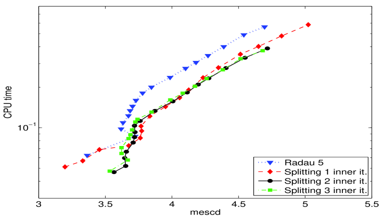
Figure 1: Work precision diagram for the Elastic Beam problem.

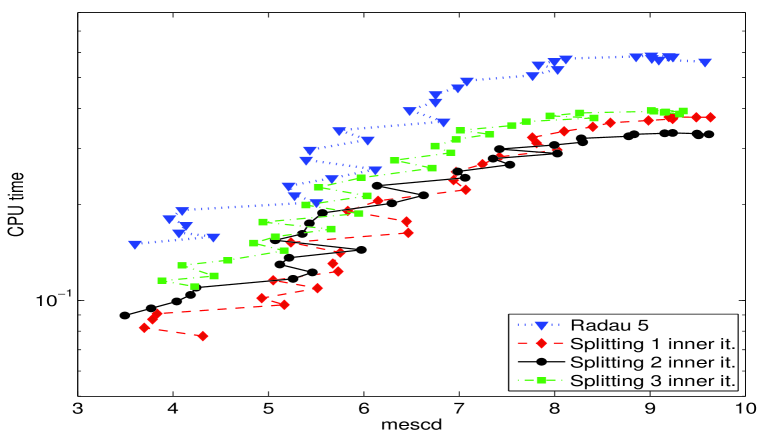
Figure 2: Work precision diagram for the Emep problem.

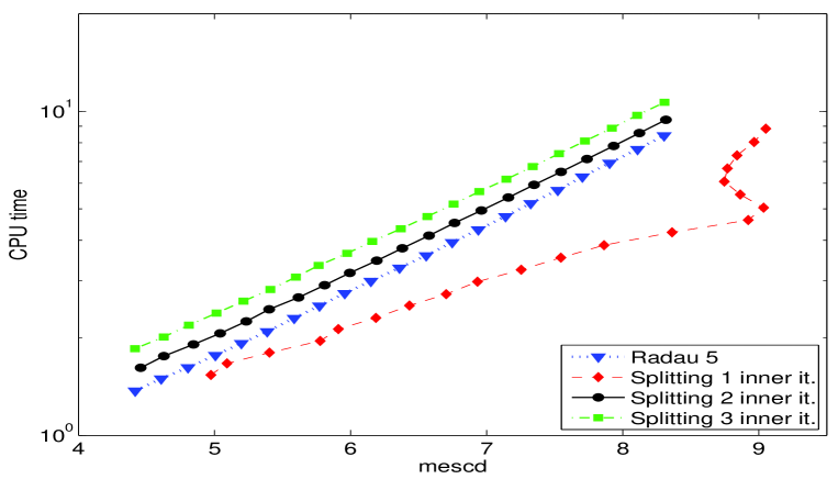
Figure 3: Work precision diagram for the Ring Modulator problem.

Table 4: Statistics for the Elastic Beam problem, RADAU5.

rtol	mescd	steps	accept	feval	jeval	LU	CPU-time
1.00E-04	3.36	55	49	380	49	55	6.24E-02
1.00E-05	3.67	112	95	764	95	112	1.23E-01
1.00E-06	3.78	162	146	1103	146	162	1.81E-01
1.00E-07	4.18	275	251	1853	251	275	3.06E-01
1.00E-08	4.69	507	459	3417	459	507	5.62E-01

Table 5: Statistics for the Elastic Beam problem, RADAU5, split 1.

rtol	mescd	steps	accept	feval	jeval	LU	CPU-time
1.00E-04	3.20	74	66	870	66	74	5.12E-02
1.00E-05	3.76	117	105	1443	105	117	8.40E-02
1.00E-06	3.95	193	177	2769	177	193	1.44E-01
1.00E-07	4.35	374	330	5925	330	374	2.80E-01
1.00E-08	5.02	801	655	12814	655	801	5.84E-01

Table 6: Statistics for the Elastic Beam problem, RADAU5, split 2.

rtol	mescd	steps	accept	feval	jeval	LU	CPU-time
1.00E-04	3.57	66	56	548	56	66	4.68E-02
1.00E-05	3.71	112	96	879	96	112	7.76E-02
1.00E-06	3.76	152	144	1290	144	152	1.12E-01
1.00E-07	4.20	284	260	2603	260	284	2.10E-01
1.00E-08	4.72	517	481	5044	481	517	3.89E-01

Table 7: Statistics for the Elastic Beam problem, RADAU5, split 3.

rtol	mescd	steps	accept	feval	jeval	LU	CPU-time
1.00E-04	3.53	64	54	454	54	64	4.76E-02
1.00E-05	3.67	115	96	810	96	115	8.32E-02
1.00E-06	3.74	154	141	1104	141	154	1.16E-01
1.00E-07	4.17	273	249	1959	249	273	2.04E-01
1.00E-08	4.68	502	456	3654	456	502	3.74E-01

Table 8: Statistics for the Ring Modulator problem, RADAU5.

rtol	mescd	steps	accept	feval	jeval	LU	CPU-time
1.00E-07	4.42	98754	89346	510295	89346	98754	1.37E+00
1.00E-08	5.20	137823	128316	727506	128316	137823	1.92E+00
1.00E-09	5.96	194463	185008	1046747	185008	194463	2.74E+00
1.00E-10	6.75	277830	268414	1525756	268414	277830	3.94E+00
1.00E-11	7.52	399846	390508	2234881	390508	399846	5.71E+00
1.00E-12	8.30	580535	571309	3365783	571309	580535	8.42E+00

Table 9: Statistics for the Ring Modulator problem, RADAU5, split 1.

rtol	mescd	steps	accept	feval	jeval	LU	CPU-time
1.00E-07	4.97	110376	95269	958749	95269	110376	1.54E+00
1.00E-08	5.91	152526	136231	1328822	136231	152526	2.13E+00
1.00E-09	6.93	212686	195982	1855438	195982	212686	2.98E+00
1.00E-10	8.36	301719	283921	2635810	283921	301719	4.23E+00
1.00E-11	8.75	432000	412643	3785978	412643	432000	6.07E+00
1.00E-12	9.05	624708	602385	5524392	602385	624708	8.84E+00

6 Conclusions

In this paper we have defined a splitting procedure for Radau IIA methods, derived by an augmented low-rank formulation of the methods. In such formulation, a set of auxiliary abscissae are determined such that the Crout factorization of a corresponding matrix associated with the method has constant diagonal entries. In such a case, the complexity of the iteration is optimal. Moreover, the presented iteration compares favorably with all previously defined iterative procedures for the efficient implementation of Radau IIA methods. The presented technique can be straightforwardly extended to other classes of implicit Runge-Kutta methods (e.g., collocation methods) and this will be the subject of future investigations.

References

- [1] R. Alexander. Diagonally implicit Runge-Kutta methods for stiff ODE’s. SIAM J. Numer. Anal. 14 (1977) 1006–1021.
- [2] P. Amodio, L. Brugnano. A Note on the Efficient Implementation of Implicit Methods for ODEs. Journal of Computational and Applied Mathematics 87 (1997) 1–9.
- [3] T.A. Bickart. An efficient solution process for implicit Runge–Kutta methods. Siam J. Numer. Anal. 14 6 (1977), 1022–1027.
- [4] L. Brugnano. Blended Block BVMs (B3VMs): A Family of Economical Implicit Methods for ODEs. Journal of Computational and Applied Mathematics 116 (2000) 41–62.
- [5] L. Brugnano, F. Iavernaro, D. Trigiante. Analisys of Hamiltonian Boundary Value Methods (HBVMs) for the numerical solution of polynomial Hamiltonian dynamical systems, 2009. arXiv:0909.5659v1
- [6] L. Brugnano, F. Iavernaro, D. Trigiante. Hamiltonian Boundary Value Methods (Energy Preserving Discrete Line Methods). Journal of Numerical Analysis, Industrial and Applied Mathematics 5 1-2 (2010) 17–37.
- [7] L. Brugnano, F. Iavernaro, D. Trigiante. A note on the efficient implementation of Hamiltonian BVMs. Journal of Computational and Applied Mathematics 236 (2011) 375–383.
- [8] L. Brugnano, F. Iavernaro, D. Trigiante. The Lack of Continuity and the Role of Infinite and Infinitesimal in Numerical Methods for ODEs: the Case of Symplecticity. Applied Mathematics and Computation 218 (2012) 8053–8063.
- [9] L. Brugnano, F. Iavernaro, D. Trigiante. A simple framework for the derivation and analysis of effective one-step methods for ODEs. Applied Mathematics and Computation 218 (2012) 8475–8485.
- [10] L. Brugnano, C. Magherini. Blended Implementation of Block Implicit Methods for ODEs. Applied Numerical Mathematics 42 (2002) 29–45.
- [11] L. Brugnano, C. Magherini. The BiM Code for the Numerical Solution of ODEs. Journal of Computational and Applied Mathematics 164-165 (2004) 145–158.
- [12] L. Brugnano, C. Magherini. Blended Implicit Methods for solving ODE and DAE problems, and their extension for second order problems. Journal of Computational and Applied Mathematics 205 (2007) 777–790.
- [13] L. Brugnano, C. Magherini. Recent Advances in Linear Analysis of Convergence for Splittings for Solving ODE problems. Applied Numerical Mathematics 59 (2009) 542–557.
- [14] L. Brugnano, C. Magherini, F. Mugnai. Blended Implicit Methods for the Numerical Solution of DAE Problems. Journal of Computational and Applied Mathematics 189 (2006) 34–50.
- [15] K. Burrage. A special family of Runge-Kutta methods for solving stiff differential equations. BIT 18 (1978) 22–41.
- [16] K. Burrage, P.M. Burrage. Low rank Runge Kutta methods, symplecticity and stochastic Hamiltonian problems with additive noise. Journal of Computational and Applied Mathematics 236 (2012) 3920–3930.
- [17] J.C. Butcher. On the implementation of implicit Runge-Kutta methods. BIT 16 (1976) 237–240.
- [18] J.C. Butcher. A transformed implicit Runge-Kutta method. J. Assoc. Comput Mach. 26 (1979) 237–240.
- [19] J.R. Cash. The integration of stiff initial value problems in ODEs using modified extended backward differentiation formulae. Comput. Math. Appl. 9 (1983) 645–657.
- [20] G.J. Cooper. On the implementation of Singly Implicit Runge-Kutta methods. Math. Comp. 57, 196 (1991) 663–672.
- [21] G.J. Cooper, J.C. Butcher. An iteration scheme for implicit Runge-Kutta methods. IMA J. Numer. Anal. 3 (1983) 127–140.
- [22] S. Gonzalez-Pinto, S. Pérez-Rodríguez, R. Rojas-Bello. Efficient iterations for Gauss methods on second order problems. J. Comput. Appl. Math. 189 (2006) 80–97.
- [23] E. Hairer, G. Wanner. Solving Ordinary Differential Equations II. Stiff and Differential-Algebraic Equations. Springer, Berlin, 1991.
- [24] E. Hairer, G. Wanner, Stiff differential equations solved by Radau methods, J. Comput. Appl. Math. 111, 1 2 (1999) 93 -111.
- [25] P.J. van der Houwen, B.P. Sommeijer. Iterated Runge–Kutta methods on parallel computers. SIAM J. Sci. Stat. Comput. 12, 5 (1991) 1000–1028.
- [26] P.J. van der Houwen, J.J.B. de Swart. Triangularly implicit iteration methods for ODE-IVP solvers. SIAM J. Sci. Comput. 18 (1997) 41–55.
- [27] P.J. van der Houwen, J.J.B. de Swart. Parallel linear system solvers for Runge-Kutta methods. Adv. Comput. Math. 7, 1-2 (1997) 157–181.
- [28] F. Iavernaro, F. Mazzia. Solving ordinary differential equations by generalized Adams methods: properties and implementation techniques. Applied Numerical Mathematics 28, 2-4 (1998) 107–126.
- [29] J.J.B. de Swart. A simple ODE solver based on 2-stage Radau IIA. Journal of Computational and Applied Mathematics 84 (1997) 227–280.
- [30] Test Set for IVP Solvers: http://www.dm.uniba.it/~testset/testsetivpsolvers/