See pages - of Pages_1a3

5.1 Introduction

Finite element methods (FEM) represent a very general set of techniques to approximate solutions of partial derivative equations. Their main advantage lies in their ability to handle arbitrary geometries via unstructured meshes of the domain of interest: The discretization of oblic geometry edges is natively built in. Finite Element Methods have been widely developed in many areas of physics and engineering: mechanics, thermodynamics…

But until the early 80’s, two major drawbacks prevented them from being used in electromagnetic problems. On the one hand, existing nodal element basis did not satisfy the physical (dis)continuity of the vector fields components and lead to spurious solutions [1]. On the other hand, there was no proper way to truncate unbounded regions in open wave problems.

These two major limitations were both overcome in the early 80’s: Vector elements have been developed by Nédélec [2, 3], and Perfectly Matched Layers (PMLs) were discovered by Bérenger [4]. Since then, it has been shown that PMLs could be described in the general framework of transformation optics [5, 6, 7, 8].

All the mathematical and computational ingredients now exist and the goal of this chapter is to show how to combine them to implement a general 3D numerical scheme adapted to gratings using Finite Elements. In fact, we are now facing the physical difficulties inherent to the infinite spatial characteristics of the grating problem, whereas the computation domain has to be bounded in practice: (i) Both the superstrate and the substrate are infinite regions, (ii) there is an infinite number of periods and, last but not least, (iii) the sources of the incident field (a plane wave) are located in the superstrate at an infinite distance from the grating.

In this chapter, the infinite extension of the superstrate and substrate is addressed using cartesian PMLs. In the framework of transformation optics, we demonstrate that Bérenger’s original PMLs can be extended to the challenging numerical cases of grazing incidence in order to deal with extreme oblic incidences or configurations near Wood’s anomalies. The second issue of infinite number of period can be addressed via Bloch conditions. Finally, we are dealing with the distant plane wave sources through an equivalence of the diffraction problem with a radiation one whose sources are localized inside the diffractive element itself. The unknown field to be approximated using Finite Elements is a radiated field with sources inside the computation box and allows to retrieve easily the total field with the plane wave source.

In a first section, we derive and implement this approach in the so-called 2D non-conical, or scalar, case. We are dealing with the infinite issues rigorously in both TE and TM polarization cases. It results in a radiation problem with sources localized in the diffractive element itself. We mathematically split the whole problem into two parts. The first one consists in the classical calculation of the total field solution of a simple interface. The second one amounts to looking for a radiated field with sources confined within the diffractive obstacles and deduced from the first elementary problem. From this viewpoint, the later radiated field can be interpreted as an exact perturbation of the total field. We show that our approach allows to tackle some kind of anisotropy without increasing the computational time or resource. Through a battery of examples, we illustrate its independence towards the geometry of the diffractive pattern. Finally, we present an Adaptative PML able to tackle grazing incidences or configurations near Wood’s anomaly.

In a second section, we extend this approach to the most general configuration of vector diffraction by crossed gratings embedded in arbitrary multilayered stack. The main advantage of this method is, again, its complete independence towards the shape of the diffractive element, whereas other methods often require heavy adjustments depending on whether the geometry of the groove region presents oblique edges. This approach combined with the use of second order edge elements allows us to retrieve the few numerical academic examples found in the literature with an excellent accuracy. Furthermore, we provide a new reference case combining major difficulties: A non trivial toroidal geometry together with strong losses and a high permittivity contrast. Finally, we discuss computation time and convergence as a function of the mesh refinement as well as the choice of the direct solver.

5.2 Scalar diffraction by arbitrary mono-dimensional gratings : a Finite Element formulation

5.2.1 Set up of the problem and notations

We denote by $\mathbf{x}$, $\mathbf{y}$ and $\mathbf{z}$, the unit vectors of the axes of an orthogonal coordinate system $Oxyz$. We deal only with time-harmonic fields; consequently, the electric and magnetic fields are represented by the complex vector fields $\mathbf{E}$ and $\mathbf{H}$, with a time dependance in $\exp(-i\,\omega\,t)$.

Besides, in this chapter, we assume that the tensor fields of relative permittivity $\underline{\underline{\varepsilon}}$ and relative permeability $\underline{\underline{\mu}}$ can be written as follows:

$$\underline{\underline{\varepsilon}}=\left(\begin{array}[]{ccc}\varepsilon_{xx}&\bar{\varepsilon}_{a}&0\\ \varepsilon_{a}&\varepsilon_{yy}&0\\ 0&0&\varepsilon_{zz}\end{array}\right)\quad\hbox{and}\quad\underline{\underline{\mu}}=\left(\begin{array}[]{ccc}\mu_{xx}&\bar{\mu}_{a}&0\\ \mu_{a}&\mu_{yy}&0\\ 0&0&\mu_{zz}\end{array}\right)\;,$$ (5.1)

where $\varepsilon_{xx},\varepsilon_{a},\dots\mu_{zz}$ are possibly complex valued functions of the two variables $x$ and $y$ and where $\bar{\varepsilon}_{a}$ (resp. $\bar{\mu}_{a}$) represents the conjugate complex of $\varepsilon_{a}$ (resp. $\mu_{a}$). These kinds of materials are said to be $z$–anisotropic. It is of importance to note that with such tensor fields, lossy materials can be studied (the lossless materials correspond to tensors with real diagonal terms represented by Hermitian matrices) and that the problem is invariant along the $z$–axis but the tensor fields can vary continuously (gradient index gratings) or discontinuously (step index gratings). Moreover we define $k_{0}:=\omega/c$.

The gratings that we are dealing with are made of three regions (See Fig. 5.1 ).

• The superstratum ($y>h^{g}$) which is supposed to be homogeneous, isotropic and lossless and characterized solely by its relative permittivity $\varepsilon^{+}$ and its relative permeability $\mu^{+}$ and we denote $k^{+}:=k_{0}\,\sqrt{\varepsilon^{+}\mu^{+}}$

• The substratum ($y<0$) which is supposed to be homogeneous and isotropic and therefore characterized by its relative permittivity $\varepsilon^{-}$ and its relative permeability $\mu^{-}$ and we denote $k^{-}:=k_{0}\,\sqrt{\varepsilon^{-}\mu^{-}}$

• The groove region ($0<y<h^{g}$) which can be heterogeneous and $z$–anisotropic and thus characterized by the two tensor fields $\underline{\underline{\varepsilon}}^{g}(x,y)$ and $\underline{\underline{\mu}}^{g}(x,y)$. It is worth noting that the method does work irrespective of whether the tensor fields are piecewise constant. The groove periodicity along $x$–axis will be denoted $d$.

Fig. 5.1: Sketch and notations of the grating studied in this section.

This grating is illuminated by an incident plane wave of wave vector $\mathbf{k}^{+}_{p}=\alpha\,\mathbf{x}-\beta^{+}\,\mathbf{y}=k^{+}\left(\sin\theta_{0}\mathbf{x}-\cos\theta_{0}\mathbf{y}\right)$, whose electric field (TM case) ( resp. magnetic field (TE case)) is linearly polarized along the $z$–axis:

$$\mathbf{E}_{e}^{0}=\mathbf{A}_{e}^{0}\,\exp(i\mathbf{k}^{+}_{p}\cdot\bm{r})\,\mathbf{z}\quad(\hbox{resp. $\mathbf{H}_{m}^{0}=\mathbf{A}_{m}^{0}\,\exp(i\mathbf{k}^{+}_{p}\cdot\bm{r})\,\mathbf{z}$})\;,$$ (5.2)

where $\mathbf{A}_{e}^{0}$ (resp. $\mathbf{A}_{m}^{0}$) is an arbitrary complex number and $\bm{r}=(x,y)^{\textrm{T}}$. In this section, a plane wave is characterized by its wave-vector denoted $\mathbf{k}^{\{+,-\}}_{\{p,c\}}$. The subscript $p$ (resp. $c$) stands for “propagative” (resp. “counter-propagative”). The superscript $+$ (resp. $-$) refers to the associated wavenumber $k^{+}$ (resp. $k^{-}$), and indicates that we are dealing with a plane wave propagating in the superstrate (resp. substrate).The magnetic (resp. electric) field derived from $\mathbf{E}_{e}^{0}$ (resp. $\mathbf{H}_{m}^{0}$) is denoted $\mathbf{H}_{e}^{0}$ (resp. $\mathbf{E}_{m}^{0}$) and the electromagnetic field associated with the incident field is therefore denoted ($\mathbf{E}^{0},\mathbf{H}^{0}$) which is equal to ($\mathbf{E}_{e}^{0},\mathbf{H}_{e}^{0}$) (resp. ($\mathbf{E}_{m}^{0},\mathbf{H}_{m}^{0}$)).

The diffraction problem that we address consists in finding Maxwell equation solutions in harmonic regime i.e. the unique solution ($\mathbf{E},\mathbf{H}$) of:

$$\mathop{\rm\mathbf{curl}}\nolimits\,\mathbf{E}=i\,\omega\,\mu_{0}\,\underline{\underline{\mu}}\,\mathbf{H}$$ (5.3a)

$$\mathop{\rm\mathbf{curl}}\nolimits\,\mathbf{H}=-i\,\omega\,\varepsilon_{0}\,\underline{\underline{\varepsilon}}\,\mathbf{E}$$ (5.3b)

such that the diffracted field $(\mathbf{E}^{\textrm{d}},\mathbf{H}^{\textrm{d}}):=(\mathbf{E}-\mathbf{E}^{0}_{e},\mathbf{H}-\mathbf{H}^{0}_{m})$ satisfies an Outgoing Waves Condition (O.W.C. [9]) and where $\mathbf{E}$ and $\mathbf{H}$ are quasi-periodic functions with respect to the $x$ coordinate.

5.2.2 Theoretical developments of the method

Decoupling of fields and $z$–anisotropy

We assume that $\underline{\underline{\delta}}(x,y)$ is a $z$–anisotropic tensor field ($\delta_{xz}=\delta_{yz}=\delta_{zx}=\delta_{zy}=0$). Moreover, the left upper matrix extracted from $\underline{\underline{\delta}}$ is denoted $\underline{\underline{\tilde{\delta}}}$, namely:

$$\underline{\underline{\tilde{\delta}}}=\left(\begin{array}[]{cc}\delta_{xx}&\bar{\delta}_{a}\\ \delta_{a}&\delta_{yy}\end{array}\right)\;.$$ (5.4)

For $z$–anisotropic materials, in a non-conical case, the problem of diffraction can be split into two fundamental cases (TE case and TM case). This property results from the following equality which can be easily derived:

$$-\mathop{\rm\mathbf{curl}}\nolimits\left({\underline{\underline{\delta}}}^{-1}\mathop{\rm\mathbf{curl}}\nolimits\left(u\,\mathbf{z}\right)\right)=\mathop{\rm div}\nolimits\left({\underline{\underline{\tilde{\delta}}}^{T}}/\det(\underline{\underline{\tilde{\delta}}})\nabla u\right)\mathbf{z}\;,$$ (5.5)

where $u$ is a function which does not depend on the $z$ variable. Relying on the previous equality, it appears that the problem of diffraction in a non conical mounting amounts to looking for an electric (resp. magnetic) field which is polarized along the $z$–axis ; $\mathbf{E}=e(x,y)\,\mathbf{z}$ (resp. $\mathbf{H}=h(x,y)\,\mathbf{z}$). The functions $e$ and $h$ are therefore solutions of similar differential equations:

$$\mathscr{L}_{\underline{\underline{\xi}},\chi}(u):=\mathop{\rm div}\nolimits\left(\underline{\underline{\xi}}\,\nabla u\right)+k_{0}^{2}\chi\,u=0$$ (5.6)

with

$$u=e,\quad\underline{\underline{\xi}}=\underline{\underline{\tilde{\mu}}}^{T}/\det(\underline{\underline{\tilde{\mu}}}),\quad\chi=\varepsilon_{zz}\;,$$ (5.7)

in the TM case and

$$u=h,\quad\underline{\underline{\xi}}=\underline{\underline{\tilde{\varepsilon}}}^{T}/\det(\underline{\underline{\tilde{\varepsilon}}}),\quad\chi=\mu_{zz}\;,$$ (5.8)

in the TE case.

Boiling down the diffraction problem to a radiation one

In its initial form, the diffraction problem summed up by Eq. (5.6) is not well suited to the Finite Element Method. In order to overcome this difficulty, we propose to split the unknown function $u$ into a sum of two functions $u_{1}$ and $u_{2}^{d}$, the first term being known as a closed form and the latter being a solution of a problem of radiation whose sources are localized within the obstacles.

We have assumed that outside the groove region (cf. Fig. 5.1), the tensor field $\underline{\underline{\xi}}$ and the function $\chi$ are constant and equal respectively to $\underline{\underline{\xi}}^{-}$ and $\chi^{-}$ in the substratum ($y<0$) and equal respectively to $\underline{\underline{\xi}}^{+}$ and $\chi^{+}$ in the superstratum ($y>h^{g}$). Besides, for the sake of clarity, the superstratum is supposed to be made of an isotropic and lossless material and is therefore solely defined by its relative permittivity $\varepsilon^{+}$ and its relative permeability $\mu^{+}$, which leads to:

$$\underline{\underline{\xi}}^{+}=\frac{1}{\mu^{+}}\,\mathrm{Id}_{2}\quad\hbox{and}\quad\chi^{+}=\varepsilon^{+}\quad\hbox{in TE case}$$ (5.9)

or

$$\underline{\underline{\xi}}^{+}=\frac{1}{\varepsilon^{+}}\,\mathrm{Id}_{2}\quad\hbox{and}\quad\chi^{+}=\mu^{+}\quad\hbox{in TM case,}$$ (5.10)

where $\mathrm{Id}_{2}$ is the $2\times 2$ identity matrix. With such notations, $\underline{\underline{\xi}}$ and $\chi$ are therefore defined as follows:

$$\underline{\underline{\xi}}(x,y):=\left\{\begin{array}[]{lcc}\underline{\underline{\xi}}^{+}&\hbox{for}&y>h^{g}\\ \underline{\underline{\xi}}^{g}(x,y)&\hbox{for}&h^{g}>y>0\\ \underline{\underline{\xi}}^{-}&\hbox{for}&y<0\end{array}\right.\;,\;\chi(x,y):=\left\{\begin{array}[]{lcc}\chi^{+}&\hbox{for}&y>h^{g}\\ \chi^{g}(x,y)&\hbox{for}&h^{g}>y>0\\ \chi^{-}&\hbox{for}&y<0\;.\end{array}\right.$$ (5.11)

It is now apropos to introduce an auxiliary tensor field $\underline{\underline{\xi}}_{1}$ and an auxiliary function $\chi_{1}$:

$$\underline{\underline{\xi}}_{1}(x,y):=\left\{\begin{array}[]{ccc}\underline{\underline{\xi}}^{+}&\hbox{for}&y>0\\ \underline{\underline{\xi}}^{-}&\hbox{for}&y<0\end{array}\right.\;,\;\chi_{1}(x,y):=\left\{\begin{array}[]{ccc}\chi^{+}&\hbox{for}&y>0\\ \chi^{-}&\hbox{for}&y<0\;,\end{array}\right.$$ (5.12)

these quantities corresponding, of course, to a simple plane interface. Besides, we introduce the constant tensor field $\underline{\underline{\xi}}_{0}$ which is equal to $\underline{\underline{\xi}}^{+}$ everywhere and a constant scalar field $\chi_{0}$ which is equal to $\chi^{+}$ everywhere. Finally, we denote $u_{0}$ the function which equals the incident field $u^{\mathrm{inc}}$ in the superstratum and vanishes elsewhere (see Fig. 5.1):

$$u_{0}(x,y):=\left\{\begin{array}[]{ccc}u^{\mathrm{inc}}&\hbox{for}&y>h^{g}\\ 0&\hbox{for}&y<h^{g}\end{array}\right.$$ (5.13)

We are now in a position to define more precisely the diffraction problem that we are dealing with. The function $u$ is the unique solution of:

$$\mathscr{L}_{\underline{\underline{\xi}},\chi}(u)=0\,,\,\,\hbox{such that $u^{d}:=u-u_{0}$ satisfies an O.W.C.}$$ (5.14)

In order to reduce this diffraction problem to a radiation problem, an intermediate function is necessary. This function, called $u_{1}$, is defined as the unique solution of the equation:

$$\mathscr{L}_{\underline{\underline{\xi}}_{1},\chi_{1}}(u_{1})=0\,,\,\,\hbox{such that $u_{1}^{d}:=u_{1}-u_{0}$ satisfies an O.W.C.}$$ (5.15)

The function $u_{1}$ corresponds thus to an annex problem associated to a simple interface and can be solved in closed form and from now on is considered as a known function. As written above, we need the function $u_{2}^{d}$ which is simply defined as the difference between $u$ and $u_{1}$:

$$u_{2}^{d}:=u-u_{1}=u^{d}-u_{1}^{d}\;.$$ (5.16)

The presence of the superscript $d$ is, of course, not irrelevant: As the difference of two diffracted fields, the O.W.C. of $u_{2}^{d}$ is guaranteed (which is of prime importance when dealing with PML cf. 5.2.2). As a result, the Eq. (5.14) becomes:

$$\mathscr{L}_{\underline{\underline{\xi}},\chi}(u_{2}^{d})=-\mathscr{L}_{\underline{\underline{\xi}},\chi}(u_{1})\;,$$ (5.17)

where the right hand member is a scalar function which may be interpreted as a known source term $-\mathscr{S}_{1}(x,y)$ and the support of this source is localized only within the groove region. To prove it, all we have to do is to use Eq. (5.15):

$$\mathscr{S}_{1}:=\mathscr{L}_{\underline{\underline{\xi}},\chi}(u_{1})=\mathscr{L}_{\underline{\underline{\xi}},\chi}(u_{1})-\underbrace{\mathscr{L}_{\underline{\underline{\xi}}_{1},\chi_{1}}(u_{1})}_{=0}=\mathscr{L}_{\underline{\underline{\xi}}-\underline{\underline{\xi}}_{1},\chi-\chi_{1}}(u_{1})\;.$$ (5.18)

Now, let us point out that the tensor fields $\underline{\underline{\xi}}$ and $\underline{\underline{\xi}}_{1}$ are identical outside the groove region and the same holds for $\chi$ and $\chi_{1}$. The support of $\mathscr{S}_{1}$ is thus localized within the groove region as expected. It remains to compute more explicitly the source term $\mathscr{S}_{1}$. Making use of the linearity of the operator $\mathscr{L}$ and the equality $u_{1}=u_{1}^{d}+u_{0}$, the source term can be split into two terms

$$\mathscr{S}_{1}=\mathscr{S}_{1}^{0}+\mathscr{S}_{1}^{d}\;,$$ (5.19)

where

$$\mathscr{S}_{1}^{0}=\mathscr{L}_{\underline{\underline{\xi}}-\underline{\underline{\xi}}_{1},\chi-\chi_{1}}(u_{0})$$ (5.20)

and

$$\mathscr{S}_{1}^{d}=\mathscr{L}_{\underline{\underline{\xi}}-\underline{\underline{\xi}}_{1},\chi-\chi_{1}}(u_{1}^{d})\;.$$ (5.21)

Now, bearing in mind that $u_{0}$ is nothing but a plane wave $u_{0}=\,\exp(i\mathbf{k}^{+}_{p}\cdot\mathbf{r})$ (with $\mathbf{k}^{+}_{p}=\alpha\mathbf{x}-\beta^{+}\mathbf{y}$), it is sufficient to give $\nabla u_{0}=i\mathbf{k}^{+}_{p}\,u_{0}$ for the weak formulation associated with Eq. (5.17):

$$\mathscr{S}_{1}^{0}=\left\{i\mathop{\rm div}\nolimits\left[\left(\underline{\underline{\xi}}^{+}-\underline{\underline{\xi}}\right)\mathbf{k}^{+}_{p}\,\exp(i\mathbf{k}^{+}_{p}\cdot\mathbf{r})\right]+k_{0}^{2}\left(\chi^{+}-\chi\right)\exp(i\mathbf{k}^{+}_{p}\cdot\mathbf{r})\right\}\;.$$ (5.22)

The same holds for the term associated with the diffracted field. Since, in the superstrate, we have of course $u_{1}^{d}=\,\rho\exp(i\mathbf{k}^{+}_{c}\cdot\mathbf{r})$ with $\mathbf{k}^{+}_{c}=\alpha\mathbf{x}+\beta^{+}\mathbf{y}$,

$$\mathscr{S}_{1}^{d}=\rho\left\{i\mathop{\rm div}\nolimits\left[\left(\underline{\underline{\xi}}^{+}-\underline{\underline{\xi}}\right)\mathbf{k}^{+}_{c}\,\exp(i\mathbf{k}^{+}_{c}\cdot\mathbf{r})\right]+k_{0}^{2}\left(\chi^{+}-\chi\right)\exp(i\mathbf{k}^{+}_{c}\cdot\mathbf{r})\right\}\;,$$ (5.23)

where $\rho$ is simply the complex reflection coefficient associated with the simple interface:

$$\rho=\frac{p^{+}-p^{-}}{p^{+}-p^{-}}\;\hbox{with}\;p^{\pm}\,=\,\left\{\begin{array}[]{ccc}\;\beta^{\pm}\;\hbox{in the TM case}\\ \\ \;\frac{\beta^{\pm}}{\varepsilon^{\pm}}\;\hbox{in the TE case}\\ \end{array}\right.$$ (5.24)

Quasi-periodicity and weak formulation

The weak formulation follows the classical lines and is based on the construction of a weighted residual of Eq. (5.6), which is multiplied by the complex conjugate of a weight function $u^{\prime}$ and integrated by part to obtain:

$$\mathscr{R}_{\underline{\underline{\xi}},\chi}(u,u^{\prime})=-\int_{\Omega}\left(\underline{\underline{\xi}}\,\nabla u\right)\cdot\nabla\overline{u^{\prime}}+k_{0}^{2}\chi\,u\;\overline{u^{\prime}}\;\textrm{d}\Omega+\int_{\partial\Omega}\overline{u^{\prime}}\left(\underline{\underline{\xi}}\,\nabla u\right)\cdot\mathbf{n}\;\textrm{d}S$$ (5.25)

The solution $u$ of the weak formulation can therefore be defined as the element of the space $L^{2}(\mathop{\rm\mathbf{curl}}\nolimits,d,\alpha)$ of quasiperiodic functions (i.e. such that $u(x,y)=u_{\#}(x,y)\,e^{i\alpha x}$ with $u_{\#}(x,y)=u_{\#}(x+d,y)$, a $d$-periodic function) of $L^{2}(\mathop{\rm\mathbf{curl}}\nolimits)$ on $\Omega$ such that:

$$\mathscr{R}_{\underline{\underline{\xi}},\chi}(u,u^{\prime})=0\;\;\forall u^{\prime}\in L^{2}(\mathop{\rm\mathbf{curl}}\nolimits,d,\alpha).$$ (5.26)

As for the boundary term introduced by the integration by part, it can be classically set to zero by imposing Dirichlet conditions on a part of the boundary (the value of $u$ is imposed and the weight function $u^{\prime}$ can be chosen equal to zero on this part of the boundary) or by imposing homogeneous Neumann conditions $(\underline{\underline{\xi}}\nabla u)\cdot\mathbf{n}=0$ on another part of the boundary (and $u$ is therefore an unknown to be determined on the boundary).

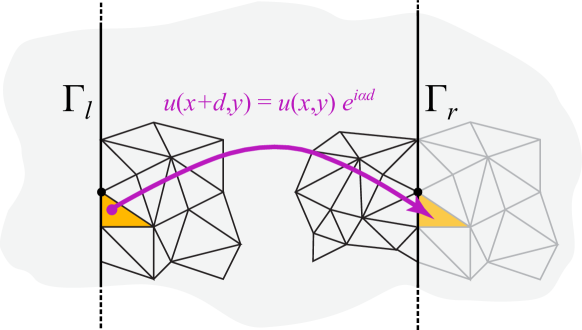
Fig. 5.2: Quasi-periodicity of the field and sample of a $d$-periodic mesh.

A third possibility are the so-called quasi-periodicity conditions of particular importance in the modeling of gratings.

Denote by $\Gamma_{l}$ and $\Gamma_{r}$ the lines parallel to the $y$–axis delimiting a cell of the grating (see Fig. 5.2) respectively from its left and right neighbor cell. Considering that both $u$ and $u^{\prime}$ are in $L^{2}(\mathop{\rm\mathbf{curl}}\nolimits,d,\alpha)$, the boundary term for $\Gamma_{l}\cup\Gamma_{r}$ is

$$\int_{\Gamma_{l}\cup\Gamma_{r}}\overline{u^{\prime}}\left(\underline{\underline{\xi}}\,\nabla u\right)\cdot\mathbf{n}\;\textrm{d}S=\int_{\Gamma_{l}\cup\Gamma_{r}}\overline{u^{\prime}_{\#}}e^{-i\alpha x}\left(\underline{\underline{\xi}}\,\nabla(u_{\#}e^{+i\alpha x})\right)\cdot\mathbf{n}\;\textrm{d}S=$$

$$\int_{\Gamma_{l}\cup\Gamma_{r}}\overline{u^{\prime}_{\#}}\left(\underline{\underline{\xi}}\,(\nabla u_{\#}+i\alpha u_{\#}\mathbf{x})\right)\cdot\mathbf{n}\;\textrm{d}S=0\,\,,$$

because the integrand $\overline{u^{\prime}_{\#}}\left(\underline{\underline{\xi}}\,(\nabla u_{\#}+i\alpha u_{\#}\mathbf{x})\right)\cdot\mathbf{n}$ is periodic along $x$ and the normal $\mathbf{n}$ has opposite directions on $\Gamma_{l}$ and $\Gamma_{r}$ so that the contributions of these two boundaries have the same absolute value with opposite signs. The contribution of the boundary terms vanishes therefore naturally in the case of quasi-periodicity.

The finite element method is based on this weak formulation and both the solution and the weight functions are classically chosen in a discrete space made of linear or quadratic Lagrange elements, i.e. piecewise first or second order two variable polynomial interpolation built on a triangular mesh of the domain $\Omega$ (cf. Fig. 5.3a). Dirichlet and Neumann conditions may be used to truncate the PML domain in a region where the field (transformed by the PML) is negligible. The quasi-periodic boundary conditions are imposed by considering the $u$ as unknown on $\Gamma_{l}$ (in a way similar to the homogeneous Neumann condition case) while, on $\Gamma_{r}$, $u$ is forced equal to the value of the corresponding point on $\Gamma_{l}$ (i.e. shifted by a quantity $-d$ along $x$) up to the factor $e^{i\alpha d}$. The practical implementation in the finite element method is described in details in [10, 11]

Perfectly Matched Layer for $z$–anisotropic materials

The main drawback encountered in electromagnetism when tackling theory of gratings through the finite element method is the non-decreasing behaviour of the propagating modes in superstratum and substratum (if they are made of lossless materials): The PML has been introduced by [4] in order to get round this obstacle. The computation of PML designed for $z$–anisotropic gratings is the topic of what follows.

In the framework of transformation optics, a PML may be seen as a change of coordinate corresponding to a complex stretch of the coordinate corresponding to the direction along which the field must decay [12, 13, 14]. Transformation optics have recently unified various techniques in computational electromagnetics such as the treatment of open problems, helicoidal geometries or the design of invisibility cloaks ([15]). These apparently different problems share the same concept of geometrical transformation, leading to equivalent material properties. A very simple and practical rule can be set up ([10]): when changing the coordinate system, all you have to do is to replace the initial materials properties $\smash{\underline{\underline{\varepsilon}}}$ and $\smash{\underline{\underline{\mu}}}$ by equivalent material properties $\smash{\underline{\underline{\varepsilon}}}_{s}$ and $\smash{\underline{\underline{\mu}}}_{s}$ given by the following rule:

$$\smash{\underline{\underline{\varepsilon}}}_{s}=\mathbf{J}^{-1}\,\smash{\underline{\underline{\varepsilon}}}\,\,\mathbf{J}^{-\rm T}\,\mathrm{det}(\mathbf{J})\hskip 5.0pt\text{and~{}}\hskip 5.0pt\smash{\underline{\underline{\mu}}}_{s}=\mathbf{J}^{-1}\,\smash{\underline{\underline{\mu}}}\,\,\mathbf{J}^{-\rm T}\,\mathrm{det}(\mathbf{J}),$$ (5.27)

where $\mathbf{J}$ is the Jacobian matrix of the coordinate transformation consisting of the partial derivatives of the new coordinates with respect to the original ones ($\mathbf{J}^{-\rm T}$ is the transposed of its inverse).
In this framework, the most natural way to define PMLs is to consider them as maps on a complex space $\mathbb{C}^{3}$, which coordinate change leads to equivalent permittivity and permeability tensors. We detail here the different coordinates used in this section.

• $(x,y,z)$ are the cartesian original coordinates.

• $(x_{s},y_{s},z_{s})$ are the complex stretched coordinates. A suitable subspace $\Gamma\subset\mathbb{C}^{3}$ is chosen (with three real dimensions) such that $(x_{s},y_{s},z_{s})$ are the complex valued coordinates of a point on $\Gamma$ (e.g. $x=\mathfrak{Re}(x_{s})$, $y=\mathfrak{Re}(y_{s})$, $z=\mathfrak{Re}(z_{s})$).

• $(x_{c},y_{c},z_{c})$ are three real coordinates corresponding to a real valued parametrization of $\Gamma\subset\mathbb{C}^{3}$.

We use rectangular PMLs ([12]) absorbing in the $y$-direction and we choose a diagonal matrix $\mathbf{J}=\mathrm{diag}(1,s_{y}(y),1)$, where $s_{y}(y)$ is a complex-valued function of the real variable $y$, defined by:

$$y_{s}(y)=\int_{0}^{y}s_{y}(y^{\prime})\rm dy^{\prime}.$$ (5.28)

The expression of the equivalent permittivity and permeability tensors are thus:

$$\smash{\underline{\underline{\varepsilon}}}_{s}=\left(\begin{array}[]{ c c c}s_{y}\varepsilon_{xx}&\overline{\varepsilon_{a}}&0\\ \varepsilon_{a}&s_{y}^{-1}\varepsilon_{yy}&0\\ 0&0&s_{y}\varepsilon_{zz}\end{array}\right)\hskip 10.0pt\text{and~{}}\hskip 10.0pt\smash{\underline{\underline{\mu}}}_{s}=\left(\begin{array}[]{ c c c}s_{y}\mu_{xx}&\overline{\mu_{a}}&0\\ \mu_{a}&s_{y}^{-1}\mu_{yy}&0\\ 0&0&s_{y}\mu_{zz}\end{array}\right).$$ (5.29)

Note that the equivalent medium has the same impedance than the original one as $\smash{\underline{\underline{\varepsilon}}}$ an $\smash{\underline{\underline{\mu}}}$ are transformed in the same way, which guarantees that the PML is perfectly reflectionless.
Now, let us define the so-called substituted field $\bm{F}_{s}=(\mathbf{E}_{s},\mathbf{H}_{s})$, solution of Eqs. (5.3) with $\smash{\underline{\underline{\xi}}}=\smash{\underline{\underline{\xi}}}_{s}$ and $\chi=\chi_{s}$. It turns out that $\bm{F}_{s}$ equals the field $\bm{F}$ in the region $y^{b}<y<y^{t}$ (with $y^{b}=-h^{-}$ and $y^{t}=h^{g}+h^{+}$, see Fig. 5.3a), provided that $s_{y}(y)=1$ in this region. The main feature of this latest field $\bm{F}_{s}$ is the remarkable correspondence with the first field $\bm{F}$ ; whatever the function $s_{y}$ provided that it equals $1$ for $y^{t}<y<y^{b}$, the two fields $\bm{F}$ and $\bm{F}_{s}$ are identical in the region $y^{t}<y<y^{b}$[8]. In other words, the PML is completely reflection-less. In addition, for complex valued functions $s_{y}$ ($\Im{\it{m}}\{s_{y}\}$ strictly positive in PML), the field $\bm{F}_{s}$ converges exponentially towards zero (as $y$ tends to $\pm\infty$, cf. Fig. 5.3c and 5.3d) although its physical counterpart $\bm{F}$ does not. Note that in Fig. 5.3d, the value of the computed radiated field $u_{2}^{d}$ on each extreme boundary of the PMLs is at least $10^{-8}$ weaker than in the region of interest. As a consequence, $\bm{F}_{s}$ is of finite energy and for this substituted field a weak formulation can be easily derived which is essential when dealing with Finite Element Method.

Still remains to give a suitable function $s_{y}$. Let us consider the complex coordinate mapping $y(y_{c})$, which is simply defined as the derivative of the stretching coefficient $s_{y}(y)$ with respect to $y_{c}$. With simple stretching functions, we can obtain a reliable criterion upon proper fields decay. A classical choice is:

$$s_{y}(y)=\begin{cases}\zeta^{-}&\mbox{if }y<y^{b}\\ 1&\mbox{if }y^{b}<y<y^{t}\\ \zeta^{+}&\mbox{if }y>y^{t}\\ \end{cases}$$ (5.30)

where $\zeta^{\pm}=\zeta^{{}^{\prime},\pm}+i\zeta^{{}^{\prime\prime},\pm}$ are complex constants with $\zeta^{{}^{\prime\prime},\pm}>0$.
In that case, the complex valued function $y(y_{c})$ defined by Eq. (5.28) is explicitly given by:

$$y(y_{c})=\begin{cases}y^{b}+\zeta^{-}(y_{c}-y^{b})&\mbox{if }y_{c}<y^{b}\\ y_{c}&\mbox{if }y^{b}<y_{c}<y^{t}\\ y^{t}+\zeta^{+}(y_{c}-y^{t})&\mbox{if }y_{c}>y^{t}\\ \end{cases},$$ (5.31)

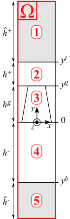
(a) Computational domain $\Omega$ and its five constituent regions.

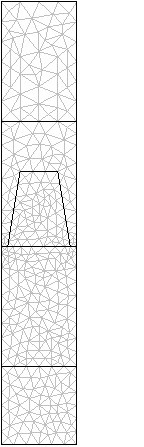
(b) Coarse triangle meshing of the cell $\Omega$. Maximum element side size: $\lambda/(2\sqrt{\varepsilon})$

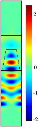
(c) Radiated field: $\Re{\it{e}}\{u_{2}^{d}\}$ in $V/m$

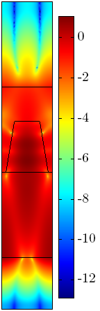
(d) Radiated field: $\log(|u_{2}^{d}|)$

Fig. 5.3: Example of computation of the radiated field $u_{2}^{d}$ (TM case).

Finally, let us consider a propagating plane wave in the substratum $u_{n}(x,y):=\exp(i(\alpha x-\beta^{-}_{n}y))$. Its expression can be rewritten as a function of the stretched coordinates in the PML as follows:

$$u^{\mathrm{sc}}_{n}(x_{c},y_{c}):=u_{n}(x(x_{c}),y(y_{c}))=e^{i\alpha x_{c}}e^{-i\beta^{-}_{n}(y^{b}+\zeta^{-}(y_{c}-y^{b}))}$$ (5.32)

The behavior of this latest function along the $y_{c}$ direction is governed by the function $U^{\mathrm{sc}}(y_{c}):=e^{-i\beta^{-}_{n}\,\zeta^{-}y_{c}}$. Letting $\beta^{\prime,-}_{n}:=\Re{\it{e}}\{\beta^{-}_{n}\}$, $\beta^{\prime\prime,-}_{n}:=\Im{\it{m}}\{\beta^{-}_{n}\}$, $\zeta^{\prime,-}:=\Re{\it{e}}\{\zeta^{-}\}$ and $\zeta^{\prime\prime,-}:=\Im{\it{m}}\{\zeta^{-}\}$, the non-oscillating part of the function $U^{\mathrm{sc}}(y_{c})$ is given by $\exp\left((\beta^{\prime,-}_{n}\,\zeta^{\prime\prime,-}\,+\beta^{\prime\prime,-}_{n}\,\zeta^{\prime,-})y_{c}\right)$. Keeping in mind that $\beta^{\prime,-}_{n}$ and/or $\beta^{\prime\prime,-}_{n}$ are positive numbers, the function $U^{\mathrm{sc}}$ decreases exponentially towards zero as $y_{c}$ tends to $-\infty$ (Fig. 5.3d) provided that $\zeta^{-}$ belongs to $\mathbb{C}^{+}:=\{z\in\mathbb{C},\Re{\it{e}}\{z\}>0,\;\hbox{and}\;\Im{\it{m}}\{z\}>0\}$. In the same way, it can be shown that $\zeta^{+}$ belongs to $\mathbb{C}^{+}$.

Let us conclude this section with two important remarks:

1. Practical choice of PML parameters. As for the complex stretch parameters, setting $\zeta^{\pm}=1+i$ is usually a safe choice. For computational needs, the PML has to be truncated and the other constitutive parameter of the PML is its thickness $\hat{h}$ (see Fig. 5.3a). Setting $\hat{h}^{\pm}=\lambda_{0}/\sqrt{\varepsilon^{\pm}}$ leads to a PML thick enough to “absorb” all incident radiation. These specific values will be used in the sequel, unless otherwise specified.

2. Special cases. The reader will notice that a configuration where $\beta^{\prime,-}_{n}$ is a very weak positive number compared to $k_{0}$ with $\beta^{\prime\prime,-}_{n}$ (this is precisely the case of a plane wave at grazing incidence on the bottom PML) leads to a very slow exponential decay of $U^{\mathrm{sc}}$. In such a case, close to so-called Wood’s anomalies or at extreme grazing incidences, classical PML fail. We will address this tricky situation extensively in Section 5.2.4.

Synthesis of the method

In order to give a general view of the method, all information is collected here that is necessary to set up the practical Finite Element Model. First of all, the computation domain $\Omega$ (cf. Fig. 5.3a) corresponds to a truncated cell of the grating which is a finite rectangle divided into five horizontal layers. These layers are respectively from top to bottom upper PML, the superstratum, the groove region, the substratum, and the lower PML. The unknown field is the scalar function $u_{2}^{d}$ defined in Eq. (5.16). Its finite element approximation is based on the second Lagrange elements built on a triangle meshing of the cell (cf. Fig. 5.3b). A complex algebraic system of linear equations is constructed via the Galerkin weighted residual method, i.e. the set of weight functions $u^{\prime}$ is chosen as the set of shape functions of interpolation on the mesh [10].

• In region $1$ (upper PML, see Fig. 5.3a),

  $$\mathscr{R}_{\underline{\underline{\xi}}_{s}^{+},\chi_{s}^{+}}(u_{2}^{d},u^{\prime})=0\;,$$ (5.33)

  with $\underline{\underline{\xi}}_{s}^{+}$ and $\chi_{s}^{+}$ depending on the equivalent anisotropic properties of the PML given by Eq. (5.7), Eq. (5.8) and Eqs. (5.29).

• In region $2$ (superstratum),

  $$\mathscr{R}_{\underline{\underline{\xi}}^{+},\chi^{+}}(u_{2}^{d},u^{\prime})=0\;,$$ (5.34)

  with $\underline{\underline{\xi}}^{+}$ and $\chi^{+}$ depending on the homogeneous isotropic properties of the superstratum given by Eq. (5.7), Eq. (5.8), Eq. (5.9) and Eq. (5.10).

• In region $3$ (groove region),

  $$\mathscr{R}_{\underline{\underline{\xi}}^{g},\chi^{g}}(u_{2}^{d},u^{\prime})=-\mathscr{R}_{\underline{\underline{\xi}}^{g},\chi^{g}}(\mathscr{S}_{1},u^{\prime})\;,$$ (5.35)

  with $\underline{\underline{\xi}}^{g}$ and $\chi^{g}$ depending on the heterogeneous possibly anisotropic properties given by Eq. (5.7), Eq. (5.8), Eq. (5.11) and $\mathscr{S}_{1}$ given by Eq. (5.19) , Eq. (5.22), Eq. (5.23) and Eq. (5.24).

• In region $4$ (substratum),

  $$\mathscr{R}_{\underline{\underline{\xi}}^{-},\chi^{-}}(u_{2}^{d},u^{\prime})=0\;,$$ (5.36)

  with $\underline{\underline{\xi}}^{-}$ and $\chi^{-}$ depending on the homogeneous isotropic properties of the substratum given by Eq. (5.7), Eq. (5.8), Eq. (5.9) and Eq. (5.10).

• In region $5$ (lower PML),

  $$\mathscr{R}_{\underline{\underline{\xi}}_{s}^{-},\chi_{s}^{-}}(u_{2}^{d},u^{\prime})=0\;,$$ (5.37)

  with $\underline{\underline{\xi}}_{s}^{-}$ and $\chi_{s}^{-}$ depending on the equivalent anisotropic properties of the PML given by Eq. (5.7), Eq. (5.8) and Eqs. (5.29).

Energy balance: Diffraction efficiencies and absorption

The rough result of the FEM calculation is the complex radiated field $u_{2}^{d}$. Using Eq. (5.16), it is straightforward to obtain the complex diffracted field $u^{d}$ solution of Eq. (5.14) at each point of the bounded domain. We deduce from $u^{d}$ the diffraction efficiencies with the following method. The superscripts ⁺ (resp. ^-) correspond to quantities defined in the superstratum (resp. substratum) as previously.

On the one hand, since $u^{d}$ is quasi-periodic along the $x$–axis , it can be expanded as a Rayleigh expansion (see for instance [9]):

$$\hbox{for}\;y<0\;\hbox{and}\;y>h^{g},\;u^{d}(x,y)=\sum_{n\in\mathbb{Z}}\,u^{d}_{n}(y)\,e^{i\alpha_{n}x}$$ (5.38)

where

$$u^{d}_{n}(y)=\frac{1}{d}\int_{-d/2}^{d/2}u^{d}(x,y)e^{-i\alpha_{n}x}\,\textrm{d}x\;\hbox{with}\;\alpha_{n}=\alpha+\frac{2\pi}{d}n$$ (5.39)

On the other hand, introducing Eq. (5.38) into Eq. (5.6) leads to the Rayleigh coefficients:

$$u^{d}_{n}(y)=\left\{\begin{array}[]{ccc}u_{n}^{+}(y)=r_{n}\,e^{\,i\beta_{n}^{+}y}+a_{n}\,e^{\,-i\beta_{n}^{+}y}&\hbox{for}&y>h^{g}\\ \\ u_{n}^{-}(y)=t_{n}\,e^{\,-i\beta_{n}^{-}y}+b_{n}\,e^{\,i\beta_{n}^{-}y}&\hbox{for}&y<0\\ \end{array}\right.\;\hbox{with}\;\beta_{n}^{\pm^{2}}=k^{\pm^{2}}-\alpha_{n}^{2}$$ (5.40)

For a temporal dependance in $e^{-i\omega t}$, the O.W.C. imposes $a_{n}=b_{n}=0$. Combining Eq. (5.39) and (5.40) at a fixed $y_{0}$ altitude leads to:

$$\left\{\begin{array}[]{ccc}r_{n}=\frac{1}{d}\displaystyle\int_{-d/2}^{d/2}u^{d}(x,y_{0})\,e^{-i(\alpha_{n}x+\beta_{n}^{+}y_{0})}\,\textrm{d}x&\hbox{for}&y_{0}>h^{g}\\ \\ t_{n}=\frac{1}{d}\displaystyle\int_{-d/2}^{d/2}u^{d}(x,y_{0})\,e^{-i(\alpha_{n}x-\beta_{n}^{-}y_{0})}\,\textrm{d}x&\hbox{for}&y_{0}<0\\ \end{array}\right.$$ (5.41)

We extract these two coefficients by trapezoidal numerical integration along $x$ from a cutting of the previously calculated field map at $y_{0}$. It is well known that the mere trapezoidal integration method is very efficient for smooth and periodic functions (integration on one period) [16]. Now the restriction on a horizontal straight line crossing the whole cell in homogeneous media (substratum and superstratum) is of $C^{\infty}$ class. From a numerical point of view, it appears that the interpolated approximation of the unknown function, namely $u_{2}^{d}$ preserves the good behaviour of the numerical computation of these integrals. From this we immediately deduce the reflected and transmitted diffracted efficiencies of propagative orders ($T_{n}$ and $R_{n}$) defined by:

$$\left\{\begin{array}[]{ccc}R_{n}:=\,r_{n}\,\overline{r_{n}}\,\frac{\beta_{n}^{+}}{\beta^{+}}&\hbox{for}&y_{0}>h^{g}\\ \\ T_{n}:=\,t_{n}\,\overline{t_{n}}\,\frac{\beta_{n}^{-}}{\beta^{-}}\,\frac{\gamma^{+}}{\gamma^{-}}&\hbox{for}&y_{0}<0\\ \end{array}\right.\hbox{with}\;\gamma^{\pm}\,=\,\left\{\begin{array}[]{ccc}1\;\hbox{in the TM case}\\ \\ \;\varepsilon^{\pm}\;\hbox{in the TE case}\\ \end{array}\right.$$ (5.42)

This calculation is performed at several different $y_{0}$ altitudes in the superstratum and the substratum, and the mean value found for each propagative transmitted or reflected diffraction order is presented in the numerical experiments of the following section.

Normalized losses $Q$ can be obtained according to Poynting’s theorem through the straightforward computation of the following ratio:

$$Q:=\frac{\displaystyle\int_{S}\omega\,\varepsilon_{0}\,\Im{\it{m}}(\varepsilon^{g^{\prime}})\,\mathbf{E}\cdot\overline{\mathbf{E}}\,\mathrm{d}s}{\displaystyle\int_{L}\Re{\it{e}}\{\mathbf{E}_{0}\times\overline{\mathbf{H}_{0}}\}\cdot\textbf{n}\,\mathrm{d}l}\,,$$ (5.43)

The numerator in Eq. (5.43) clarifies losses in Watts by period of the considered grating and are computed by integrating the Joule effect losses density over the surface $S$ of the lossy element. The denominator normalizes these losses to the incident power, i.e. the time-averaged incident Poynting vector flux across one period (a straight line $L$ of length $d$ in the superstrate parallel to $Ox$, whose normal oriented along decreasing values of $y$ is denoted n).

Finally, combining Eqs. (5.42) and Eq. (5.43), a self consistency check of the whole numerical scheme consists in comparing the quantity $B$:

$$B:=\displaystyle\sum_{n}T_{n}+\sum_{m}R_{m}+Q$$ (5.44)

to unity. In Eq. (5.44), the summation indexed by $n$ (resp. $m$) corresponds to the sum over the efficiencies of all transmitted (resp. reflected) propagative diffraction orders in the substrate (resp. superstrate). We give interpretations and concrete examples of such numerical energy balances over non trivial grating profiles in sections 5.2.3 and 5.2.3.

5.2.3 Numerical experiments

Numerical validation of the method

We can refer to [17] in order to test the accuracy of our method. The studied grating is isotropic, since we lack numerical values in the literature in anisotropic cases. We compute the following problem (cf. Fig. 5.4), as described in [18] and [17]. The wavelength of the plane wave is set to $1\,\mu m$ and is incoming with an angle of $\pi/6$ with respect to the normal to the grating.

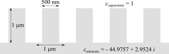
Fig. 5.4: Rectangular groove grating: This pattern is repeatedly set up with a period $d$ = 1 $\mu m$. This grating has been studied by [17] and is one of our points of reference

Maximum element size	$R_{0}^{\mathrm{TE}}$	$R_{0}^{\mathrm{TM}}$
$\lambda_{0}/(4\,\sqrt{\epsilon})$	0.7336765	0.8532342
$\lambda_{0}/(6\,\sqrt{\epsilon})$	0.7371302	0.8456592
$\lambda_{0}/(8\,\sqrt{\epsilon})$	0.7347466	0.8482817
$\lambda_{0}/(10\,\sqrt{\epsilon})$	0.7333739	0.850071
$\lambda_{0}/(12\,\sqrt{\epsilon})$	0.7346569	0.8494844
$\lambda_{0}/(14\,\sqrt{\epsilon})$	0.7341944	0.8483238
$\lambda_{0}/(16\,\sqrt{\epsilon})$	0.7342714	0.8484774
Result given by [17]	0.7342789	0.8484781

Tab. 5.1: Reflected efficiencies versus mesh refinement. Note that the efficiencies are properly computed (two significant digits) even for a rather coarse mesh.

We present the $R_{0}$ efficiency (cf. Table 5.1) in both cases of polarization versus the mesh refinement. So we have a good agreement to the reference values, and the accuracy reached is independent from the polarization case.

Experiment set up based on existing materials

The method proposed in this section is adapted to $z$–anisotropic materials, such as transparent $\textrm{CaCO}_{3}$ [19], $\textrm{LiNbO}_{3}$ [20] or Ni:YIG [21] and lossy CoPt or CoPd [22]. Let us now consider a trapezoidal (cf. Fig. 5.5) anisotropic grating made of aragonite ($\textrm{CaCO}_{3}$) deposited on an isotropic substratum ($\textrm{SiO}_{2}$, $\varepsilon_{\,\mathrm{SiO_{2}}}=2.25$). Along the anisotropic crystal axis, its dielectric tensor can be written as follows [19]:

$$\underline{\underline{\varepsilon}}_{\,\textrm{CaCO}_{3}}=\left(\begin{array}[]{ccc}2.843&0&0\\ 0&2.341&0\\ 0&0&2.829\end{array}\right)\quad\hbox{and}\quad\underline{\underline{\mu}}_{\,\mathrm{CaCO_{3}}}=\left(\begin{array}[]{ccc}\mu_{0}&0&0\\ 0&\mu_{0}&0\\ 0&0&\mu_{0}\end{array}\right)\;$$ (5.45)

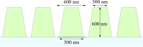
Fig. 5.5: Diffractive element pattern. This element is made of aragonite for which the dielectric tensor is given by Eq. (5.46) and is deposited on a silica substrate with a period $d=600\,\textrm{nm}$.

Now let’s assume that the natural axis of our aragonite grating are rotated by $45^{\,\circ}$ around the grating infinite dimension. The dielectric tensor becomes:

$$\underline{\underline{\varepsilon}}_{\,\textrm{CaCO}_{3}}^{45^{\,\circ}}=\left(\begin{array}[]{ccc}2.592&0.251&0\\ 0.251&2.592&0\\ 0&0&2.829\end{array}\right)$$ (5.46)

We shall here remind that our method remains strictly the same whatever the diffractive element geometry is. The 2D computational domain is bounded along the $y$–axis by the PMLs and along the $x$ since we consider only one pseudo period. We propose to calculate the diffractive efficiencies at $\lambda_{0}=633\,\textrm{nm}$ in both polarization cases TE and TM, and for different incoming incidences ($0^{\,\circ}$, $20^{\,\circ}$ and $40^{\,\circ}$). Since both $\underline{\underline{\mu}}$ and $\underline{\underline{\varepsilon}}$ are Hermitian, the whole incident energy is diffracted and the sum of theses efficiencies ought to be equal to the incident energy, which will stand for validation of our numerical calculation.

Finally, the resulting bounded domain is meshed with a maximum mesh element side size of $\lambda_{0}/10\,\sqrt{\varepsilon}$. Efficiencies are still post-processed in accordance with the calculation presented section 5.2.2.

TM                 TE

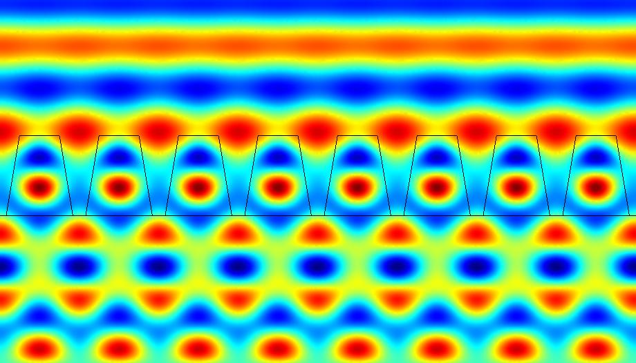
(a) $\Re{\it{e}}\{e\}$ in $V/m$ at $\theta_{0}\,=\,0^{\,\circ}$

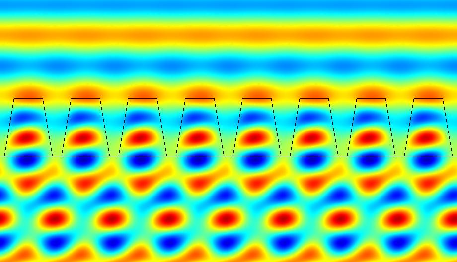
(b) $\Re{\it{e}}\{h\}$ in $A/m$ at $\theta_{0}\,=\,0^{\,\circ}$

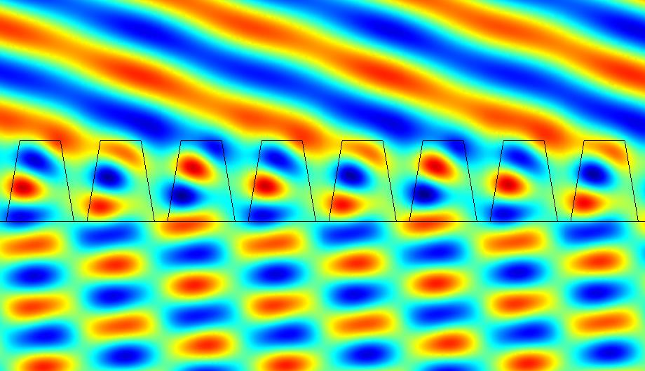
(c) $\Re{\it{e}}\{e\}$ in $V/m$ at $\theta_{0}\,=\,20^{\,\circ}$

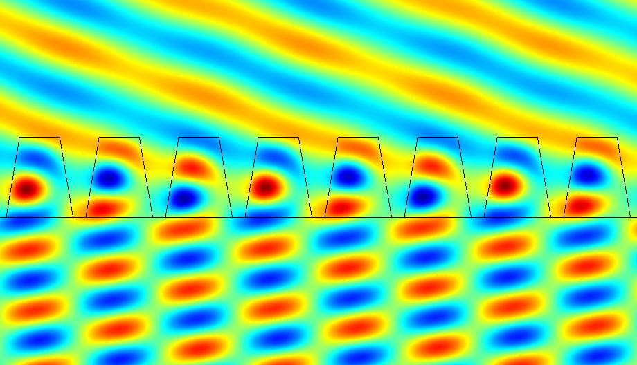
(d) $\Re{\it{e}}\{h\}$ in $A/m$ at $\theta_{0}\,=\,20^{\,\circ}$

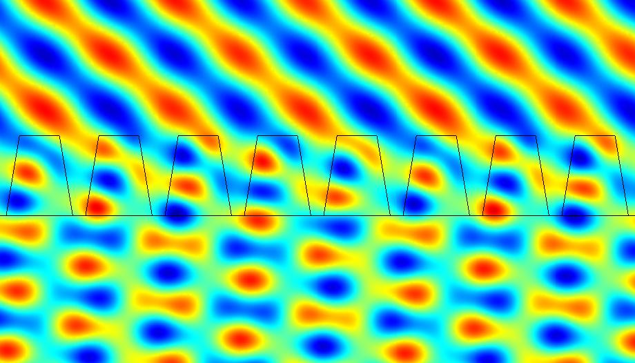
(e) $\Re{\it{e}}\{e\}$ in $V/m$ at $\theta_{0}\,=\,40^{\,\circ}$

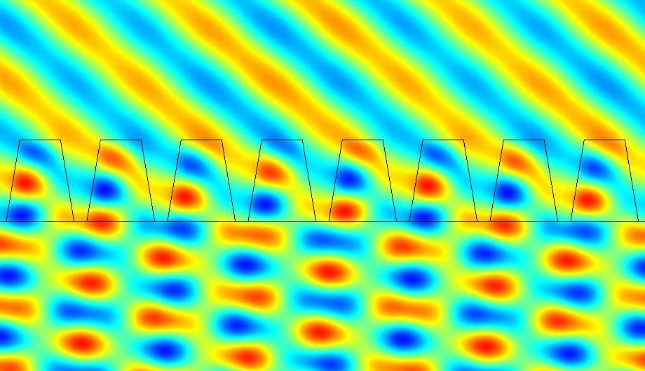
(f) $\Re{\it{e}}\{h\}$ in $A/m$ at $\theta_{0}\,=\,40^{\,\circ}$

Fig. 5.6: Real part of the total calculated field depending on $\theta_{0}$ and the polarization case

TM	$T_{-2}$	$T_{-1}$	$T_{0}$	$T_{1}$	$R_{-1}$	$R_{0}$	$R_{1}$	total
$0^{\,\circ}$	-	0.203133	0.585235	0.203138	-	0.008473	-	0.999978
$20^{\,\circ}$	-	0.399719	0.575625	0.004643	0.004412	0.015630	-	1.000029
$40^{\,\circ}$	0.025047	0.420714	0.493491	-	0.002541	0.058238	-	1.000031
TE	$T_{-2}$	$T_{-1}$	$T_{0}$	$T_{1}$	$R_{-1}$	$R_{0}$	$R_{1}$	total
$0^{\,\circ}$	-	0.322510	0.538165	0.124722	-	0.014683	-	1.000080
$20^{\,\circ}$	-	0.538727	0.444403	0.000369	0.005372	0.011180	-	1.000051
$40^{\,\circ}$	0.012058	0.434191	0.541090	-	0.005032	0.007686	-	1.000057

Tab. 5.2: Transmitted and reflected efficiencies of propagative orders deduced from field maps shown Fig. 5.6

At normal incidence, the $h$ field in the TE case (cf. Fig. 5.6b) is non symmetric whereas the $e$ field in the TM case is (cf. Fig. 5.6a). This is illustrated by the obvious non-symmetry of $T_{-1}^{\mathrm{TE}}$ and $T_{1}^{\mathrm{TE}}$ (cf. Table 5.2: 0.322510 versus 0.124722!), whereas $T_{-1}^{\mathrm{TM}}=T_{1}^{\mathrm{TM}}=0.20313$.

A non trivial geometry

Since the beginning of this chapter, we have laid great stress upon the independence of the method towards the geometry of the pattern. But we have considered so far diffractive objects of simple trapezoidal section. Let us tackle a way more challenging case and see what this approach is made of.

We can obtain an quite winding shape by extracting the contrast contour of an arbitrary image (see Fig. 5.7a-5.7b). The contour is approximated by a set of splines, and the resulting domain is finely meshed (Fig. 5.7c). Finally, as shown in Fig. 5.7b, the formed pattern ($h^{g}/\lambda_{0}=1.68$), breathing in free space ($\varepsilon_{\textrm{substrat}}=1$), is supposed to be periodically repeated $d/\lambda_{0}=1.26$ on a plane ground of glass ($\varepsilon_{\textrm{SiO}_{2}}=2.25$). The element is considered to be “made of” a lossy material of high optical index ($\varepsilon_{\textrm{marsu}}=40+0.1\,i$). The response of this system to a incident s-polarized plane wave at oblic incidence ($\theta_{0}=-30^{\circ}$) is finally calculated. The real part of the quasi-periodic total field is represented in Fig. 5.7d for three periods.

Indeed, we do not have any tabulated data available to check our results. But what we do have is a pretty reliable consistency check through the computation of the energy balance described by Eqs. (5.42) and (5.43). As shown in Fig. 5.7e, we obtain at least 7 significative digits on the energetic values. The total balance of 1.00000019 is computed taking into account (i) values of the total field inside the diffractive elements, (ii) values of the diffracted field at altitudes spanning the whole (modeled) superstrate, (iii) values of the total field at altitudes spanning the entire (modeled) substrate. Finally, (iv) the calculated field $u_{2}^{d}$ also nicely decays exponentially inside both PML. These four points allow us to check a posteriori the validity of the field everywhere in the computation cell.

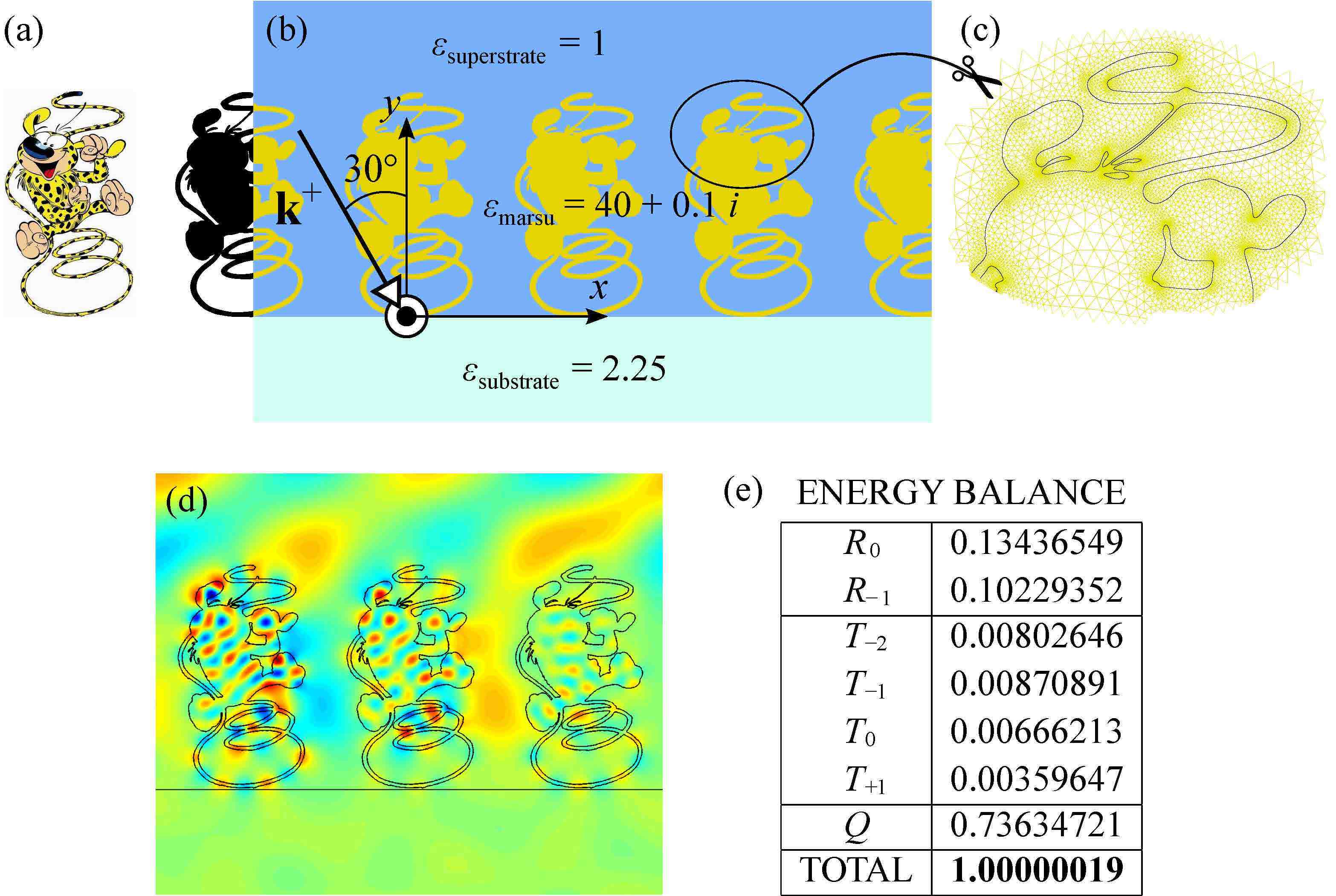
Fig. 5.7: (a) Initial contrasted image. (b) Proposed set up. (c) Sample mesh. (d) $\Re e\{E_{z}\}$ in $V/m$. (e) Energy balance of the problem.

5.2.4 Dealing with Wood anomalies using Adaptative PML

As we have noticed at the end of Section 5.2.2, PMLs based on “traditional coordinate stretching” are inefficient for periodic problems when dealing with grazing angles of diffracted orders, i.e. when the frequency is near a Wood’s anomaly ([23, 24]), leading to spurious reflexions and thus numerical pollution of the results. An important question in designing absorbing layers is thus the choice of their parameters: The PML thickness and the absorption coefficient. To this aim, adaptative formulations have already been set up, most of them employing a posteriori error estimate [25, 18, 26]. In this section, we propose Adaptative PMLs (APMLs) with a suitable coordinate stretching, depending both on incidence and grating parameters, capable of efficiently absorbing propagating waves with nearly grazing angles. This section is dedicated to the mathematical formulation used to determine PML parameters adapted to any diffraction orders. We provide at the end a numerical example of a dielectric slit grating showing the relevance of our approach in comparison with classical PMLs.

Skin depth of the PML

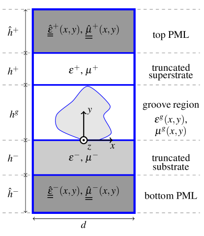
Fig. 5.8: The basic cell used for the FEM computation of the diffracted field $u_{2}^{d}$.

As explained in Section 5.2.2, the diffracted field $u^{d}$ can be expanded as a Rayleigh expansion, i.e. into an infinite sum of propagating and evanescent plane waves called diffraction orders. As detailed at the end of Section 5.2.2, we are now in position to rewrite easily the expression of, say, a transmitted diffraction order into the substrate. Similar considerations also apply to the reflected orders in the top PML. Combining Eq. (5.32) and (5.40) lead to the expression $u_{n,s}^{-}(y_{c})$ of a transmitted propagative order inside the PML:

$$u_{n,s}^{-}(y_{c})=u_{n}^{-}(y(y_{c}))=t_{n}\mathbf{e}^{-i\beta_{n}^{-}[y^{t}+\zeta^{-}(y_{c}-y^{t})]}.$$

The non oscillating part of this function is given by:

$$U_{n}^{-}(y)=t_{n}\exp{\left((\beta^{\prime,-}_{n}\zeta^{\prime\prime,-}+\beta^{\prime\prime,-}_{n}\zeta^{\prime,-})y_{c}\right)},$$

where $\beta_{n}^{-}=\beta^{\prime,-}_{n}+i\beta^{\prime\prime,-}_{n}$. For a propagating order we have $\beta^{\prime,-}_{n}>0$ and $\beta^{\prime,-}_{n}=0$, while for an evanescent order $\beta^{\prime,-}_{n}=0$ and $\beta^{\prime\prime,-}_{n}>0$. It is thus sufficient to take $\zeta^{\prime,-}>0$ and $\zeta^{\prime\prime,-}>0$ to ensure the exponential decay to zero of the field inside the PML if it was of infinite extent. But, of course, for practical purposes, the thickness of the PML is finite and has to be suitably chosen. Two pitfalls must be avoided:

1. The PML thickness is chosen too small compared to the skin depth. As a consequence, the electromagnetic wave cannot be considered as vanishing: An incident electromagnetic “sees the bottom of the PML”. In other words, this PML of finite thickness is no longer reflection-less.

2. The PML thickness is chosen much larger than the skin depth. In that case, a significant part of the PML is not useful, which gives rise to the resolution of linear systems of unnecessarily large dimensions.

Then remains to derive the skin depth, $l_{n}^{-}$, associated with the propagating order $n$. This characteristic length is defined as the depth below the PML at which the field falls to $1/e$ of its value near the surface:

$$U_{n}^{-}(y-l_{n}^{-})=\frac{U_{n}^{-}(y)}{e}.$$

Finally, we find $l_{n}^{-}=(\beta^{\prime,-}_{n}\zeta^{\prime\prime,-}+\beta^{\prime\prime,-}_{n}\zeta^{\prime,-})^{-1}$ and we define $l^{-}$ as the largest value among the $l_{n}^{-}$:

$$l^{-}=\underset{n\in\mathbb{Z}}{\mathrm{max}}\,l_{n}^{-}.$$

The height of the bottom PML region is set to $\hat{h}^{-}=10l^{-}$.

Weakness of the classical PML for grazing diffracted angles

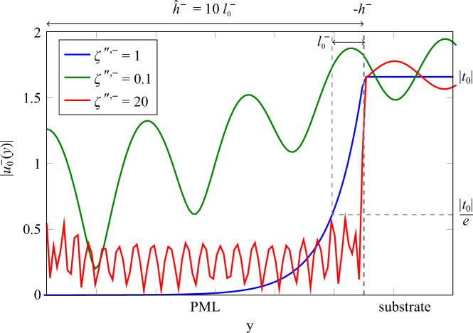
Fig. 5.9: Zero^th transmitted order by a grating with a rectangular cross section (see parameters in text, part 5.2.4) for different values of $\zeta^{\prime\prime,-}$: blue line, $\zeta^{\prime\prime,-}=1$, correct damping; green line, $\zeta^{\prime\prime,-}=0.1$, underdamping; red line, $\zeta^{\prime\prime,-}=20$, overdamping.

Let us consider the (bottom) PML adapted to the substrate. Similar conclusions will hold for the top PML. The efficiency of the classical PML fails for grazing diffracted angles, in other words when a given order appears/vanishes: this is the so-called Wood’s anomaly, well known in the grating theory. In mathematical terms, there exists $n_{0}$ such that $\beta_{n_{0}}^{-}\simeq 0$. The skin depth of the PML then becomes very large. To compensate this, it is tempting to increase the value of $\zeta^{\prime\prime,-}$, but it would lead to spurious numerical reflections due to an overdamping. For a fixed value of $\hat{h}^{-}$, if $\zeta^{\prime\prime,-}$ is too weak, the absorption in the PMLs is insufficient and the wave is reflected on the outward boundary of the PML. To illustrate these typical behaviors (cf. Fig. 5.9), we compute the field diffracted by a grating with a rectangular cross section of height $h^{g}=1.5\,\hbox{\textmu}\textrm{m}$ and width $L^{g}=3\,\hbox{\textmu}\textrm{m}$ with $\varepsilon^{g}=11.7$, deposited on a substrate with permittivity $\varepsilon^{-}=2.25$. The structure is illuminated by a p-polarized plane wave of wavelength $\lambda_{0}=10\,\hbox{\textmu}\textrm{m}$ and of angle of incidence $\theta_{0}=10^{\circ}$ in the air ($\varepsilon^{+}=1$). All materials are non magnetic ($\mu_{r}=1$) and the periodicity of the grating is $d=4\,\hbox{\textmu}\textrm{m}$. We set $\hat{h}^{-}=10l_{0}^{-}$ and $\zeta^{\prime,-}=1$.

Construction of an adaptative PML

To overcome the problems pointed out in the previous section, we propose a coordinate stretching that rigorously treats the problem of Wood’s anomalies. The wavelengths “seen” by the system are very different depending on the order at stake:

• if the diffracted angle $\theta_{n}$ is zero, the apparent wavelength $\lambda_{0}/\cos\theta_{n}$ is simply the incident wavelength,

• if the diffracted angle is near $\pm\pi/2$ (grazing angle), the apparent wavelength $\lambda_{0}/\cos\theta_{n}$ is very large.

Thus if a classical PML is adapted to one diffracted order, it will not be for another, and vice versa. The idea behind the APML is to deal with each and every order when progressing in the absorbing medium.

Once again the development will be conducted only for the PML adapted to the substrate. We consider a real-valued coordinate mapping $y_{d}(y)$, the final complex-valued mapping is then $y_{c}(y)=\zeta^{-}y_{d}(y)$, with the complex constant $\zeta^{-}$, with $\zeta^{\prime,-}>0$ and $\zeta^{\prime\prime,-}>0$, accounting for the damping of the PML medium.

We begin with transforming the equation ${\beta_{n}^{\pm}}^{2}={k^{\pm}}^{2}-{\alpha_{n}^{\pm}}^{2}$, so that the function with integer argument $n\mapsto\beta_{n}^{-}$ becomes a function with real argument continuously interpolated between the imposed integer values. Indeed, the geometric transformations associated to the PML has to be continuous and differentiable in order to compute its Jacobian. To that extent, we choose the parametrization:

$$\alpha(y_{d})=\alpha_{0}+\frac{2\pi}{d}\frac{y_{d}}{\lambda_{0}},$$ (5.47)

so that the application $\beta^{-}$ defined by ${\beta^{-}(y_{d})}^{2}=k_{0}^{2}\varepsilon^{-}-{\alpha(y_{d})}^{2}$ is continuous. Thus, the propagation constant of the $n^{\text{th}}$ transmitted order is given by $\beta_{n}^{-}=\beta^{-}(n\lambda_{0})$. The key idea is to combine the complex stretching with a real non uniform contraction (given by the continuous function $y(y_{d})$, Eq. (5.49)). This contraction is chosen in such a way that for each order $n$ there is a depth $y_{d}^{n}$ such that, around this depth, the apparent wavelength corresponding to the order in play is contracted to a value close to $\lambda_{0}$. At that point of the PML, this order is perfectly absorbed thanks to the complex stretch. We thus eliminate first the orders with quasi normal diffracted angles at lowest depths up to grazing orders (near Wood’s anomalies) which are absorbed at greater depths. In mathematical words, the translation of previous considerations on the real contraction can be expressed as:

$$\exp{[-i\beta^{-}(y_{d})y(y_{d})]}=\exp{(-ik_{0}y_{d})}$$ (5.48)

The contraction $y(y_{d})$ is thus given by:

$$y(y_{d})=\frac{k_{0}y_{d}}{\beta^{-}(y_{d})}=\frac{y_{d}}{\sqrt{\varepsilon^{-}-(\sin{\theta_{0}}+y_{d}/d)^{2}}}$$ (5.49)

The function $y(y_{d})$ has two poles, denoted $y_{d,\pm}^{\star}=d(\pm\sqrt{\varepsilon^{-}}-\sin{\theta_{0}})$. When $y_{d,\pm}^{\star}=\pm n\lambda_{0}$ with $n\in\mathbb{N}^{\star}$, $\beta^{-}(y_{d,\pm}^{\star})=\beta^{-}(\pm n\lambda_{0})=\beta_{\pm}^{-}=0$, i.e. we are on a Wood’s anomaly associated with the appearance/disappearance of the $\pm n^{\text{th}}$ transmitted order. We now search for the nearest point to $y_{d,\pm}^{*}$ associated with a Wood’s anomaly, denoting:

$$\begin{cases}n_{+}^{\star}/\quad D_{+}=\underset{n_{+}^{\star}\in\mathbb{N}^{\star}}{\mathrm{min}}\,|y_{d,+}^{\star}-n_{+}^{\star}\lambda_{0}|\\ \\ n_{-}^{\star}/\quad D_{-}=\underset{n_{-}^{\star}\in\mathbb{N}^{\star}}{\mathrm{min}}\,|y_{d,-}^{\star}+n_{-}^{\star}\lambda_{0}|\end{cases}\,\,.$$

In a second step, we look for the point $y_{d}^{0}=n^{\star}\lambda_{0}$ such that:

$$n^{\star}/\quad D=\underset{n^{\star}\in\{n_{+}^{\star},n_{-}^{\star}\}}{\mathrm{min}}\,(D^{+},D^{-})\,\,.$$ (5.50)

To avoid the singular behaviour at $y_{d}=y_{d,\pm}^{\star}$, we continue the graph of the function $y_{d}(y)$ by a straight line tangent at $y_{d}^{0}$, which equation is $t_{0}(y_{d})=s(y_{d}^{0})(y_{d}-y_{d}^{0})+y(y_{d}^{0})$, where $s(y_{d})=\frac{\partial y}{\partial y_{d}}(y_{d})$ is the so-called stretching coefficient. The final change of coordinate is then given by :

$$\tilde{y}(y_{d})=\begin{cases}y(y_{d})\mbox{ for }y_{d}\leq y_{d}^{0}\\ \\ t_{0}(y_{d})\mbox{ for }y_{d}>y_{d}^{0}.\end{cases}$$ (5.51)

Figure 5.10 shows an example of this coordinate mapping.

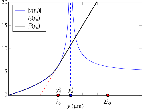
Fig. 5.10: Example of a coordinate mapping $\tilde{y}(y_{d})$ used for the APML (black solid line). The graph of $y_{d}(y)$ (blue solid line) is continued by a straight line $t_{0}(y_{d})$ tangent at $y_{d}^{0}$ (red dashed line) to avoid the singular behaviour at $y_{d}=y_{d}^{\star}$.

Eventually, the complex stretch $s_{y}$ used in Eq. (5.29) is given by:

$$s_{y}(y_{d})=\zeta^{-}\frac{\partial\tilde{y}}{\partial y_{d}}(y_{d}).$$ (5.52)

Equipped with this mathematical formulation, we can tailor a layer that is doubly perfectly matched:

• to a given medium, which is the aim of the PML technique, through Eq. (5.27),

• to all diffraction orders, through the stretching coefficient $s_{y}$, which depends on the characteristics of the incident wave and on opto-geometric parameters of the grating.

Numerical example

We now apply the method described in the preceding parts to design an adapted bottom PML for the same example as in part 5.2.4. The parameters are the same, and we choose the wavelength of the incident plane wave close to the Wood’s anomaly related to the $+1$ transmitted order ($\lambda_{0}=0.999y_{d,+}^{\star}$).Moreover, we set the length of the PML $\hat{h}^{-}=1.1y_{d,+}^{\star}$ and choose absorption coefficients $\zeta^{+}=\zeta^{-}=1+i$. For both cases (PML and APML), parameters are alike, the only difference being the complex stretch $s_{y}$.

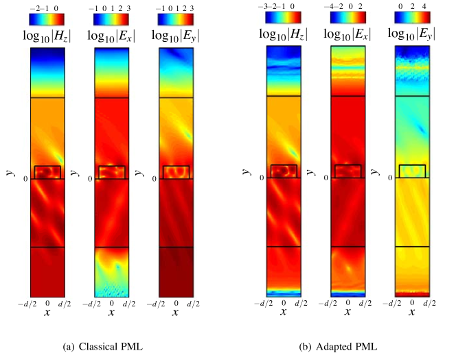
Fig. 5.11: Field maps of the logarithm of the norm of $H_{z}$, $E_{x}$ and $E_{y}$ for the dielectric slit grating at $\lambda_{0}=0.999y_{d,+}^{\star}$ (same parameters as in part 5.2.4). (a): classical PML with inefficient damping of $H_{z}$ in the bottom PML. (b): APML where the $H_{z}$ field is correctly damped in the bottom PML. For both cases the thickness of the PML is $\hat{h}^{-}=1.1y_{d,+}^{\star}$.

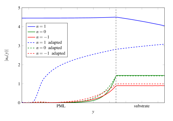
Fig. 5.12: Modulus of the $u_{n}$ for the three propagating orders with adapted (dashed lines) and classical PMLs (solid lines). Note that the classical PMLs are efficient for all orders except for the grazing one ($n=1$) as expected. This drawback is bypassed when using the adaptative PML.

The field maps of the norm of $H_{z}$, $E_{x}$ and $E_{y}$ are plotted in logarithmic scale on Fig. 5.11, for the case of a classical PML and our APML. We can observe that the field $H_{z}$ that is effectively computed is clearly damped in the bottom APML (leftmost on Fig. 5.11(b)) whereas it is not in the standard case (leftmost on Fig. 5.11(a)), causing spurious reflections on the outer boundary. The fields $E_{x}$ and $E_{y}$ are deduced from $H_{z}$ thanks to Maxwell’s equations. The high values of $E_{y}$ at the tip of the APML (rightmost on Fig. 5.11(b)) are due to very high values of the optical equivalent properties of the APML medium (due to high values of $s_{y}$), which does not affect the accuracy of the computed field within the domain of interest.
Another feature of our approach is that it efficiently absorbs the grazing diffraction order, as illustrated on Fig. 5.12: the $+1$ transmitted order does not decrease in the standard PML (blue solid line), and reaches a high value at $y=-\hat{h}^{-}$, whereas the same order tends to zero as $y\rightarrow-\hat{h}^{-}$ in the case of the adapted PML (blue dashed line).
To further validate the accuracy of the method, we compare the diffraction efficiencies computed by our FEM formulation with PML and APML to those obtained by another method. We choose the Rigorous Coupled Wave Analysis (RCWA), also known as the Fourier Modal Method (FMM, [27]). For the chosen parameters, only the $0$^th order is propagative in reflexion and the orders $-1$, $0$ and $+1$ are non evanescent in transmission. We can also check the energy balance $B=R_{0}+T_{-1}+T_{0}+T_{+1}$ since there is no lossy medium in our example. Results are reported in Table 5.3, and show a good agreement of the FEM with APML with the results from RCWA. On the contrary, if classical PML are used, the diffraction efficiencies are less accurate compared to those computed with RCWA. Checking the energy balance leads the same conclusions: the numerical result is perturbed by the reflection of the waves at the end of the PML if it is not adapted to the situation of nearly grazing diffracted orders.

	$R_{0}$	$T_{-1}$	$T_{0}$	$T_{+1}$	$B$
RCWA	0.1570	0.3966	0.1783	0.2680	0.9999
FEM + APML	0.1561	0.3959	0.1776	0.2703	0.9999
FEM + PML	0.1904	0.4118	0.1927	0.2481	1.0430

Tab. 5.3: Diffraction efficiencies $R_{0}$, $T_{-1}$, $T_{0}$ and $T_{+1}$ of the four propagating orders, and energy balance $B=R_{0}+T_{-1}+T_{0}+T_{+1}$, computed by three methods: RCWA (line 1), FEM formulation with APML (line 2), FEM formulation with classical PML (line 3).

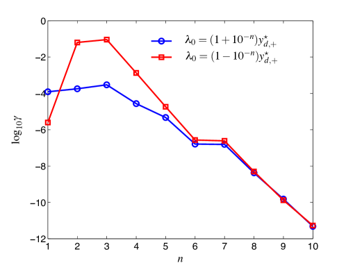
Fig. 5.13: Mean value of the norm of $H_{z}$ along the outer boundary of the bottom PML $\gamma=\langle|H_{z}(-\hat{h}^{-})|\rangle_{x}$, for $\lambda_{0}$ approaching the Wood’s anomaly $y_{d,+}^{\star}$ by inferior values ($\lambda_{0}=(1-10^{-n})y_{d,+}^{\star}$, red squares) and by superior value ($\lambda_{0}=(1+10^{-n})y_{d,+}^{\star}$, blue circles) as a function of $n$.

Eventually, to illustrate the behavior of the adaptative PML when the incident wavelength gets closer to a given Wood’s anomaly, we computed the mean value of the norm of $H_{z}$ along the outer boundary of the bottom PML $\gamma=\langle|H_{z}(-\hat{h}^{-})|\rangle_{x}$, when $\lambda_{0}=(1+10^{-n})y_{d,+}^{\star}$ and $\lambda_{0}=(1-10^{-n})y_{d,+}^{\star}$, for $n=1,2,...10$. The results are shown in Fig. 5.13. As the wavelength gets closer to $y_{d,+}^{\star}$, $\gamma$ first increases but for $n>3$, it decreases exponentially. However, in all cases, the value of $\gamma$ remains small enough to ensure the efficiency of the PMLs.

5.2.5 Concluding remarks

A novel FEM formulation was adapted to the analysis of z-anisotropic gratings relying on a rigorous treatment of the plane wave sources problem through an equivalent radiation problem with localized sources. The developed approach presents the advantage of being very general in the sense that it is applicable to every conceivable grating geometry.

Numerical experiments based on existing materials at normal and oblique incidences in both TE and TM cases showed the efficiency and the accuracy of our method. We demonstrated we could generate strongly imbalanced symmetric propagative orders in the TE polarization case and at normal incidence with an aragonite grating on a silica substratum.

We also introduced the adaptative PML for grazing incidences configurations. It based on a complex-valued coordinate stretching that deals with grazing diffracted orders, yielding an efficient absorption of the field inside the PML. We provided an example in the TM polarization case (but similar results hold for the TE case), illustrating the efficiency of our method. The value of the magnetic field on the outward boundary of the PML remains small enough to consider there is no spurious reflection. The formulation is used with the FEM but can be applied to others numerical methods. Moreover, the generalization to the vectorial three-dimensional case is straightforward: the recipes given in this last section do work irrespective of the dimension and whether the problem is vectorial.

In the next section, the scalar formulation adapted to mono-dimensional gratings is extended to the the most general case of bi-dimensional grating embedded in an arbitrary multilayered dielectric stack with arbitrary incidence.

5.3 Diffraction by arbitrary crossed-gratings : a vector Finite Element formulation

5.3.1 Introduction

In this section, we extend the method detailed in Sec. 5.2 to the most general case of vector diffraction by an arbitrary crossed gratings. The main advantage of the Finite Element Method lies in its native ability to handle unstructured meshes, resulting in a build-in accurate discretization of oblique edges. Consequently, our approach remains independent of the shape of the diffractive element, whereas other methods require heavy adjustments depending on whether the geometry of the groove region presents oblique edges (e.g. RCWA [28], FDTD…). In this section, for the sake of clarity, we recall again the rigorous procedure allowing to deal with the issue of the plane wave sources through an equivalence of the diffraction problem with a radiation one whose sources are localized inside the diffractive element itself, as already proposed in Sec. 5.2 [29, 30].

This approach combined with the use of second order edge elements allowed us to retrieve with a good accuracy the few numerical academic examples found in the literature. Furthermore, we provide a new reference case combining major difficulties such as a non trivial toroidal geometry together with strong losses and a high permittivity contrast. Finally, we discuss computation time and convergence as a function of the mesh refinement as well as the choice of the direct solver.

5.3.2 Theoretical developments

Set up of the problem and notations

We denote by $\mathbf{x}$, $\mathbf{y}$ and $\mathbf{z}$ the unit vectors of the axes of an orthogonal coordinate system $Oxyz$. We only deal with time-harmonic fields; consequently, electric and magnetic fields are represented by the complex vector fields $\mathbf{E}$ and $\mathbf{H}$, with a time dependance in $\exp(-i\,\omega\,t)$. Note that incident light is now propagating along the $z$-axis, whereas $y$-axis was used in the 2D case.

Besides, in this section, for the sake of simplicity, the materials are assumed to be isotropic and therefore are optically characterized by their relative permittivity $\varepsilon$ and relative permeability $\mu$ (note that the inverse of relative permeabilities are denoted here ${\color[rgb]{0,0,0}\nu}$). It is of importance to note that lossy materials can be studied, the relative permittivity and relative permeability being represented by complex valued functions. The crossed-gratings we are dealing with can be split into the following regions as suggested in Fig. 5.14:

• The superstrate ($z>z_{0}$) is supposed to be homogeneous, isotropic and lossless, and therefore characterized by its relative permittivity $\varepsilon^{+}$ and its relative permeability $\mu^{+}(=1/{\color[rgb]{0,0,0}\nu}^{+})$ and we denote $k^{+}:=k_{0}\,\sqrt{\varepsilon^{+}\mu^{+}}$, where $k_{0}:=\omega/c$,

• The multilayered stack ($z_{N}<z<z_{0}$) is made of $N$ layers which are supposed to be homogeneous and isotropic, and therefore characterized by their relative permittivity $\varepsilon^{n}$, their relative permeability $\mu^{n}(=1/{\color[rgb]{0,0,0}\nu}^{n})$ and their thickness $e_{n}$. We denote $k_{n}:=~{}k_{0}\,\sqrt{\varepsilon^{n}\,\mu^{n}}$ for $n$ integer between $1$ and $N$.

• The groove region ($z_{g}<z<z_{g-1}$), which is embedded in the layer indexed $g$ $(\varepsilon^{g},\mu^{g})$ of the previously described domain, is heterogeneous. Moreover the method does work irrespective of whether the diffractive elements are homogeneous: The permittivity and permeability can vary continuously (gradient index gratings) or discontinuously (step index gratings). This region is thus characterized by the scalar fields $\varepsilon^{g^{\prime}}(x,y,z)$ and $\mu^{g^{\prime}}(x,y,z)(=1/{\color[rgb]{0,0,0}\nu}^{g^{\prime}}(x,y,z))$. The groove periodicity along the $x$–axis, respectively (resp.) $y$–axis, is denoted $d_{x}$, resp. $d_{y}$, in the sequel.

• The substrate ($z<z_{N}$) is supposed to be homogeneous and isotropic and therefore characterized by its relative permittivity $\varepsilon^{-}$ and its relative permeability $\mu^{-}(=1/{\color[rgb]{0,0,0}\nu}^{-})$ and we denote $k^{-}:=k_{0}\,\sqrt{\varepsilon^{-}\mu^{-}}$,

Let us emphasize the fact that the method principles remain unchanged in the case of several diffractive patterns made of distinct geometry and/or material.

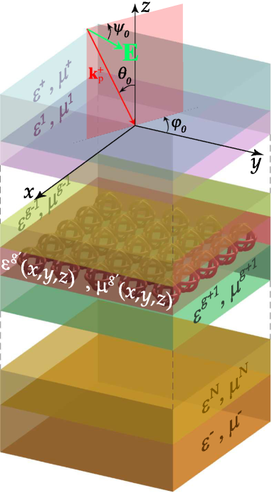
Fig. 5.14: Scheme and notations of the studied bi-gratings.

The incident field on this structure is denoted:

$$\mathbf{E}^{\mathrm{inc}}=\textbf{A}_{0}^{e}\;\textrm{exp}(i\,\textbf{k}^{+}_{p}\cdot\textbf{r})$$ (5.53)

with

$$\textbf{k}^{+}=\left[\begin{array}[]{l}\alpha_{0}\\ \beta_{0}\\ \gamma_{0}\end{array}\right]=k^{+}\,\left[\begin{array}[]{l}-\sin\theta_{0}\,\cos\varphi_{0}\\ -\sin\theta_{0}\,\sin\varphi_{0}\\ -\cos\theta_{0}\end{array}\right]$$ (5.54)

and

$$\textbf{A}_{0}^{e}=\left[\begin{array}[]{l}E^{0}_{x}\\ E^{0}_{y}\\ E^{0}_{z}\end{array}\right]=A^{e}\,\left[\begin{array}[]{l}\cos\psi_{0}\,\cos\theta_{0}\,\cos\varphi_{0}-\sin\psi_{0}\,\sin\varphi_{0}\\ \cos\psi_{0}\,\cos\theta_{0}\,\sin\varphi_{0}+\sin\psi_{0}\,\cos\varphi_{0}\\ -\cos\psi_{0}\,\sin\theta_{0}\end{array}\right],$$ (5.55)

where $\varphi_{0}\in[0,2\pi]$, $\theta_{0}\in[0,\pi/2]$ and $\psi_{0}\in[0,\pi]$ (polarization angle).

We recall here the diffraction problem: finding the solution of Maxwell equations in harmonic regime i.e. the unique solution ($\mathbf{E},\mathbf{H}$) of:

$$\mathop{\rm\mathbf{curl}}\nolimits\,\mathbf{E}=i\,\omega\,\mu_{0}\,\mu\,\mathbf{H}$$ (5.56a)

$$\mathop{\rm\mathbf{curl}}\nolimits\,\mathbf{H}=-i\,\omega\,\varepsilon_{0}\,\varepsilon\,\mathbf{E}$$ (5.56b)

such that the diffracted field satisfies the so-called Outgoing Waves Condition (OWC [31] ) and where $\mathbf{E}$ and $\mathbf{H}$ are quasi-bi-periodic functions with respect to $x$ and $y$ coordinates.

One can choose to calculate arbitrarily $\mathbf{E}$, since $\mathbf{H}$ can be deduced from Eq. (5.56a). The diffraction problem amounts to looking for the unique solution $\mathbf{E}$ of the so-called vectorial Helmholtz propagation equation, deduced from Eqs. (5.56a,5.56b):

$$\mathscr{M}_{\varepsilon,{\color[rgb]{0,0,0}\nu}}:=-\mathop{\rm\mathbf{curl}}\nolimits\left({\color[rgb]{0,0,0}\nu}\,\mathop{\rm\mathbf{curl}}\nolimits\mathbf{E}\right)+k_{0}^{2}\,\varepsilon\,\mathbf{E}=\textbf{0}$$ (5.57)

such that the diffracted field satisfies an OWC and where $\mathbf{E}$ is a quasi-bi-periodic function with respect to $x$ and $y$ coordinates.

From a diffraction problem to a radiative one with localized sources

According to Fig. 5.14, the scalar relative permittivity $\varepsilon$ and inverse permeability ${\color[rgb]{0,0,0}\nu}$ fields associated to the studied diffractive structure can be written using complex-valued functions defined by part and taking into account the notations adopted in Sec. 5.3.2:

$$\upsilon(x,y,z):=\left\{\begin{array}[]{lcccc}\upsilon^{+}&\hbox{for}&z>z_{0}&&\\ \upsilon^{n}&\hbox{for}&z_{n-1}>z>z_{n}&\hbox{with}&1\leq n<g\\ \upsilon^{g^{\prime}}(x,y,z)&\hbox{for}&z_{g-1}>z>z_{g}&&\\ \upsilon^{n}&\hbox{for}&z_{n-1}>z>z_{n}&\hbox{with}&g<n\leq N\\ \upsilon^{-}&\hbox{for}&z<z_{N}&&\end{array}\right.$$ (5.58)

with $\upsilon=\{\varepsilon,{\color[rgb]{0,0,0}\nu}\}\quad,\quad z_{0}=0\quad\textrm{and}\quad z_{n}=-\sum_{l=1}^{n}e_{l}\quad\textrm{for}\quad 1\leq n\leq N$.

It is now convenient to introduce two functions defined by part $\varepsilon_{1}$ and ${\color[rgb]{0,0,0}\nu}_{1}$ corresponding to the associated multilayered case (i.e. the same stack without any diffractive element) constant over $Ox$ and $Oy$:

$$\upsilon_{1}(x,y,z):=\left\{\begin{array}[]{lcccc}\upsilon^{+}&\hbox{for}&z>0\\ \upsilon^{n}&\hbox{for}&z_{n-1}>z>z_{n}&\hbox{with}&1\leq n\leq N\\ \upsilon^{-}&\hbox{for}&z<z_{N}\end{array}\right.$$ (5.59)

with $\upsilon=\{\varepsilon,{\color[rgb]{0,0,0}\nu}\}$.

We denote by $\mathbf{E}_{0}$ the restriction of $\mathbf{E}^{\mathrm{inc}}$ to the superstrate region:

$$\mathbf{E}_{0}:=\left\{\begin{array}[]{ccc}\mathbf{E}^{\mathrm{inc}}&\hbox{for}&z>z_{0}\\ \mathbf{0}&\hbox{for}&z\leq z_{0}\end{array}\right.$$ (5.60)

We are now in a position to define more explicitly the vector diffraction problem that we are dealing with in this section. It amounts to looking for the unique vector field $\mathbf{E}$ solution of:

$$\mathscr{M}_{\varepsilon,{\color[rgb]{0,0,0}\nu}}(\mathbf{E})=\mathbf{0}\quad\hbox{such that $\mathbf{E}^{d}:=\mathbf{E}-\mathbf{E}_{0}$ satisfies an OWC.}$$ (5.61)

In order to reduce this diffraction problem to a radiation one, an intermediary vector field denoted $\mathbf{E}_{1}$ is necessary and is defined as the unique solution of:

$$\mathscr{M}_{\varepsilon_{1},{\color[rgb]{0,0,0}\nu}_{1}}(\mathbf{E}_{1})=\mathbf{0}\quad\hbox{such that $\mathbf{E}_{1}^{d}:=\mathbf{E}_{1}-\mathbf{E}_{0}$ satisfies an OWC.}$$ (5.62)

The vector field $\mathbf{E}_{1}$ corresponds to an ancillary problem associated to the general vectorial case of a multilayered stack which can be calculated independently. This general calculation is seldom treated in the literature, we present a development in Appendix. Thus $\mathbf{E}_{1}$ is from now on considered as a known vector field. It is now apropos to introduce the unknown vector field $\mathbf{E}_{2}^{d}$, simply defined as the difference between $\mathbf{E}$ and $\mathbf{E}_{1}$, which can finally be calculated thanks to the FEM and:

$$\mathbf{E}_{2}^{d}:=\mathbf{E}-\mathbf{E}_{1}=\mathbf{E}^{d}-\mathbf{E}_{1}^{d}\;.$$ (5.63)

It is of importance to note that the presence of the superscript $d$ is not fortuitous: As a difference between two diffracted fields (Eq. (5.63), $\mathbf{E}_{2}^{d}$ satisfies an OWC which is of prime importance in our formulation. By taking into account these new definitions, Eq. (5.61) can be written:

$$\mathscr{M}_{\varepsilon,{\color[rgb]{0,0,0}\nu}}(\mathbf{E}_{2}^{d})=-\mathscr{M}_{\varepsilon,{\color[rgb]{0,0,0}\nu}}(\mathbf{E}_{1})\;,$$ (5.64)

where the right-hand member is a vector field which can be interpreted as a known vectorial source term $-\mathscr{S}_{1}(x,y,z)$ whose support is localized inside the diffractive element itself. To prove it, let us introduce the null term defined in Eq. (5.62) and make the use of the linearity of $\mathscr{M}$, which leads to:

$$\mathscr{S}_{1}:=\mathscr{M}_{\varepsilon,{\color[rgb]{0,0,0}\nu}}(\mathbf{E}_{1})=\mathscr{M}_{\varepsilon,{\color[rgb]{0,0,0}\nu}}(\mathbf{E}_{1})-\underbrace{\mathscr{M}_{\varepsilon_{1},{\color[rgb]{0,0,0}\nu}_{1}}(\mathbf{E}_{1})}_{=\mathbf{0}}=\mathscr{M}_{\varepsilon-\varepsilon_{1},{\color[rgb]{0,0,0}\nu}-{\color[rgb]{0,0,0}\nu}_{1}}(\mathbf{E}_{1})\;.$$ (5.65)

Quasi-periodicity and weak formulation

The weak form is obtained by multiplying scalarly Eq. (5.61) by weighted vectors $\mathbf{E}^{\prime}$ chosen among the ensemble of quasi-bi-periodic vector fields of $L^{2}(\mathop{\rm\mathbf{curl}}\nolimits)$ (denoted $L^{2}\left(\mathop{\rm\mathbf{curl}}\nolimits,(d_{x},d_{y}),\mathbf{k}\right)$) in $\Omega$:

$$\mathscr{R}_{\varepsilon,{\color[rgb]{0,0,0}\nu}}(\mathbf{E},\mathbf{E}^{\prime})=\int_{\Omega}-\mathop{\rm\mathbf{curl}}\nolimits\left({\color[rgb]{0,0,0}\nu}\,\mathop{\rm\mathbf{curl}}\nolimits\mathbf{E}\right)\cdot\overline{\mathbf{E}^{\prime}}+k_{0}^{2}\,\varepsilon\,\mathbf{E}\cdot\overline{\mathbf{E}^{\prime}}\,\mathrm{d}\Omega$$ (5.66)

Integrating by part Eq. (5.66) and making the use of the Green-Ostrogradsky theorem lead to:

$$\mathscr{R}_{\varepsilon,{\color[rgb]{0,0,0}\nu}}(\mathbf{E},\mathbf{E}^{\prime})=\int_{\Omega}-{\color[rgb]{0,0,0}\nu}\,\mathop{\rm\mathbf{curl}}\nolimits\mathbf{E}\cdot\mathop{\rm\mathbf{curl}}\nolimits\overline{\mathbf{E}^{\prime}}+k_{0}^{2}\,\varepsilon\,\mathbf{E}\cdot\overline{\mathbf{E}^{\prime}}\,\mathrm{d}\Omega-\int_{\partial\Omega}\left(\textbf{n}\times({\color[rgb]{0,0,0}\nu}\,\mathop{\rm\mathbf{curl}}\nolimits\mathbf{E})\right)\cdot\overline{\mathbf{E}^{\prime}}\,\mathrm{d}S$$ (5.67)

where n refers to the exterior unit vector normal to the surface $\partial\Omega$ enclosing $\Omega$.

The first term of this sum concerns the volume behavior of the unknown vector field whereas the right-hand term can be used to set boundary conditions (Dirichlet, Neumann or so called quasi-periodic Bloch-Floquet conditions).

The solution $\mathbf{E}_{2}^{d}$ of the weak form associated to the diffraction problem, expressed in its previously defined equivalent radiative form at Eq. (5.64), is the element of $L^{2}\left(\mathop{\rm\mathbf{curl}}\nolimits,(d_{x},d_{y}),\mathbf{k}\right)$ such that:

$$\forall\mathbf{E}^{\prime}\in L^{2}(\mathop{\rm\mathbf{curl}}\nolimits,d_{x},d_{y},\mathbf{k}),\,\mathscr{R}_{\varepsilon,\nu}(\mathbf{E}_{2}^{d},\mathbf{E}^{\prime})=-\mathscr{R}_{\varepsilon-\varepsilon_{1},\nu-\nu_{1}}(\mathbf{E}_{1},\mathbf{E}^{\prime})\,.$$ (5.68)

In order to rigorously truncate the computation a set of Bloch boundary conditions are imposed on the pair of planes defined by $(y=-d_{y}/2,y=d_{y}/2)$ and $(x=-d_{x}/2,x=d_{x}/2)$. One can refer to [11] for a detailed implementation of Bloch conditions adapted to the FEM. A set of Perfectly Matched Layers are used in order to truncate the substrate and the superstrate along $z$ axis (see [32] for practical implementation of PML adapted to the FEM). Since the proposed unknown $\mathbf{E}_{2}^{d}$ is quasi-bi-periodic and satisfies an OWC, this set of boundary conditions is perfectly reasonable: $\mathbf{E}_{2}^{d}$ is radiated from the diffractive element towards the infinite regions of the problem and decays exponentially inside the PMLs along $z$ axis. The total field associated to the diffraction problem $\mathbf{E}$ is deduced at once from Eq. (5.63).

Edge or Whitney 1-form second order elements

In the vectorial case, edge elements (or Whitney forms) make a much more relevant choice [33] than nodal elements. Note that a lot of work (see for instance [34]) has been done on higher order edge elements since their introduction by Bossavit [35]. These elements are suitable to the representation of vector fields such as $\mathbf{E}_{2}^{d}$, by letting their normal component be discontinuous and imposing the continuity of their tangential components. Instead of linking the Degrees Of Freedom (DOF) of the final algebraic system to the nodes of the mesh, the DOF associated to edges (resp. faces) elements are the circulations (resp. flux) of the unknown vector field along (resp. across) its edges (resp. faces).

Let us consider the computation cell $\Omega$ together with its exterior boundary $\partial\Omega$. This volume is sampled in a finite number of tetrahedron according to the following rules: Two distinct tetrahedrons have to either share a node, an edge or a face or have no contact. Let us denote by $\mathcal{T}$ the set of tetrahedrons, $\mathcal{F}$ the set of faces, $\mathcal{E}$ the set of edges and $\mathcal{N}$ the set of nodes. In the sequel, one will refers to the node $n=\{i\}$, the edge $e=\{i,j\}$, the face $f=\{i,j,k\}$ and the tetrahedron $t=\{i,j,k,l\}$.

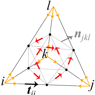
Fig. 5.15: Degrees of freedom of a second order tetrahedral element.

Twelve DOF (two for each of the six edges of a tetrahedron) are classically derived from line integral of weighted projection of the field $\mathbf{E}_{2}^{d}$ on each oriented edge $e=\{i,j\}$:

$$\left\{\begin{array}[]{c}\vartheta_{ij}=\displaystyle\int_{i}^{j}\mathbf{E}_{2}^{d}\cdot\textbf{t}_{ij}\,\lambda_{i}\,\textrm{d}l\\ \vartheta_{ji}=\displaystyle\int_{j}^{i}\mathbf{E}_{2}^{d}\cdot\textbf{t}_{ji}\,\lambda_{j}\,\textrm{d}l\end{array}\right.,$$ (5.69)

where $\textbf{t}_{ij}$ is the unit vector and $\lambda_{i}$, the barycentric coordinate of node $i$, is the chosen weight function.

According to Yioultsis et al. [36], a judicious choice for the remaining DOF is to make the use of a tangential projection of the 1-form $\mathbf{E}_{2}^{d}$ on the face $f=\{i,j,k\}$.

$$\left\{\begin{array}[]{c}\vartheta_{ijk}=\displaystyle\int_{f}\left(\mathbf{E}_{2}^{d}\times\textbf{n}_{ijk}^{+}\right)\cdot\mathop{\rm\mathbf{grad}}\nolimits\lambda_{j}\,\textrm{d}s\\ \vartheta_{ikj}=\displaystyle\int_{f}\left(\mathbf{E}_{2}^{d}\times\textbf{n}_{ijk}^{-}\right)\cdot\mathop{\rm\mathbf{grad}}\nolimits\lambda_{k}\,\textrm{d}s\end{array}\right..$$ (5.70)

The expressions for the shape functions, or basis vectors, of the second order 1-form Whitney element are given by:

$$\left\{\begin{array}[]{cl}\textbf{w}_{ij}&=(8\,\lambda_{i}^{2}-4\,\lambda_{i})\,\mathop{\rm\mathbf{grad}}\nolimits\lambda_{j}+(-8\,\lambda_{i}\,\lambda_{j}+2\,\lambda_{j})\,\mathop{\rm\mathbf{grad}}\nolimits\lambda_{i}\\ \textbf{w}_{ijk}&=16\,\lambda_{i}\,\lambda_{j}\,\mathop{\rm\mathbf{grad}}\nolimits\lambda_{k}-8\,\lambda_{j}\,\lambda_{k}\,\mathop{\rm\mathbf{grad}}\nolimits\lambda_{i}-8\,\lambda_{k}\,\lambda_{i}\,\mathop{\rm\mathbf{grad}}\nolimits\lambda_{j}\end{array}\right..$$ (5.71)

This choice of shape function ensures [37] the following fundamental property: every degree of freedom associated with a shape function should be zero for any other shape function. Finally, an approximation of the unknown $\mathbf{E}_{2}^{d}$ projected on the shape functions of the mesh $m$ ($\mathbf{E}_{2}^{d,m}$) can be derived:

$$\mathbf{E}_{2}^{d,m}=\sum_{e\in\mathcal{E}}\vartheta_{e}\,\textbf{w}_{e}+\sum_{f\in\mathcal{F}}\vartheta_{f}\,\textbf{w}_{f}.$$ (5.72)

Weight functions $\mathbf{E}^{\prime}$ (c.f. Eq. (5.68) are chosen in the same space than the unknown $\mathbf{E}_{2}^{d}$, $L^{2}(\mathop{\rm\mathbf{curl}}\nolimits,(d_{x},d_{y}),\mathbf{k})$. According to the Galerkin formulation, this choice is made so that their restriction to one bi-period belongs to the set of shape functions mentioned above. Inserting the decomposition of $\mathbf{E}_{2}^{d}$ of Eq. (5.72) in Eq. (5.68) leads to the final algebraic system which is solved, in the following numerical examples, thanks to direct solvers.

5.3.3 Energetic considerations: Diffraction efficiencies and losses

Contrarily to modal methods based on the determination of Rayleigh coefficients, the rough results of the FEM are three complex components of the vector field $\mathbf{E}^{d}$ interpolated over the mesh of the computation cell. Diffraction efficiencies are deduced from this field maps as follows.

As a difference between two quasi-periodic vector fields (see Eq. (5.61)), $\mathbf{E}^{d}$ is quasi-bi-periodic and its components can be expanded as a double Rayleigh sum:

$$E^{d}_{x}(x,y,z)=\sum_{(n,m)\in\mathbb{Z}^{2}}u_{n,m}^{d,x}(z)\,e^{{\color[rgb]{0,0,0}i\,(\alpha_{n}\,x+\beta_{m}\,y)}},$$ (5.73)

with $\alpha_{n}=\alpha_{0}+\frac{2\,\pi}{d_{x}}\,n$, $\beta_{m}=\beta_{0}+\frac{2\,\pi}{d_{y}}\,m$ and

$$u_{n,m}^{d,x}(z)=\frac{1}{d_{x}\,d_{y}}\int_{-d_{x}/2}^{d_{x}/2}\int_{-d_{y}/2}^{d_{y}/2}E_{x}^{d}(x,y,z)\,e^{-i\,(\alpha_{n}\,x+\beta_{m}\,y)}\,\mathrm{d}x\,\mathrm{d}y\,.$$ (5.74)

By inserting the decomposition of Eq. (5.73), which is satisfied by $E_{x}^{d}$ everywhere but in the groove region, into the Helmholtz propagation equation, one can express Rayleigh coefficients in the substrate and the superstrate as follows:

$$u_{n,m}^{d,x}(z)=e_{n,m}^{x,p}\,e^{\,-i\,\gamma_{n,m}^{+}\,z}+e_{n,m}^{x,c}\,e^{\,i\,\gamma_{n,m}^{+}\,z}$$ (5.75)

with $\gamma_{n,m}^{\pm^{2}}=k^{\pm^{2}}-\alpha_{n}^{2}-\beta_{m}^{2}$, where $\gamma_{n,m}$ (or $-i\,\gamma_{n,m}$) is positive. The quantity $u_{n,m}^{d,x}$ is the sum of a propagative plane wave (which propagates towards decreasing values of $z$, superscript $p$) and of a counterpropagative one (superscript $c$). The OWC verified by $\mathbf{E}^{d}$ imposes:

$$\forall(n,m)\in\mathbb{Z}^{2}\left\{\begin{array}[]{c}e_{n,m}^{x,p}=0\quad\hbox{for}\quad z>z_{0}\\ e_{n,m}^{x,c}=0\quad\hbox{for}\quad z<z_{N}\\ \end{array}\right.$$ (5.76)

Eq. (5.74) allows to evaluate numerically $e_{n,m}^{x,c}$ (resp. $e_{n,m}^{x,p}$) by double trapezoidal integration of a slice of the complex component $E^{d}_{x}$ at an altitude $z_{c}$ fixed in the superstrate (resp. substrate). It is well known that the mere trapezoidal integration method is very efficient for smooth and periodic functions (integration on one period). The same holds for $E_{y}^{d}$ and $E_{z}^{d}$ components as well as their coefficients $e_{n,m}^{y,\{c,p\}}$ and $e_{n,m}^{z,\{c,p\}}$.

The dimensionless expression of the efficiency of each reflected and transmitted $(n,m)$ order [38] is deduced from Eqs. (5.75,5.76):

$$\left\{\begin{array}[]{ccc}R_{n,m}={\color[rgb]{0,0,0}\frac{1}{|A_{e}|^{2}}}\,\displaystyle\frac{\gamma_{n,m}^{+}}{\gamma_{0}}\,\textbf{e}_{n,m}^{c}(z_{c})\cdot\overline{\textbf{e}_{n,m}^{c}(z_{c})}\quad\hbox{for}\quad z_{c}>z_{0}\\ T_{n,m}={\color[rgb]{0,0,0}\frac{1}{A_{e}^{2}}}\,\displaystyle\frac{\gamma_{n,m}^{-}}{\gamma_{0}}\,\textbf{e}_{n,m}^{p}(z_{c})\cdot\overline{\textbf{e}_{n,m}^{p}(z_{c})}\quad\hbox{for}\quad z_{c}<z_{N}\\ \end{array}\right.,$$ (5.77)

with $\textbf{e}_{n,m}^{\{c,p\}}=e_{n,m}^{x,\{c,p\}}\,\textbf{x}+e_{n,m}^{y,\{c,p\}}\,\textbf{y}+e_{n,m}^{z,\{c,p\}}\,\textbf{z}$.

Furthermore, normalized losses Q can be obtained through the computation of the following ratio:

$$Q=\frac{\displaystyle\int_{V}\frac{1}{2}\,\omega\,\varepsilon_{0}\,\Im{\it{m}}(\varepsilon^{g^{\prime}})\,\mathbf{E}\cdot\overline{\mathbf{E}}\,\mathrm{d}V}{\displaystyle\int_{S}\frac{1}{2}\Re{\it{e}}\{\mathbf{E}_{0}\times\overline{\mathbf{H}_{0}}\}\cdot\textbf{n}\,\mathrm{d}S}\,.$$ (5.78)

The numerator in Eq. (5.78) clarifies losses in watts by bi-period of the considered crossed-grating and are computed by integrating the Joule effect losses density over the volume $V$ of the lossy element. The denominator normalizes these losses to the incident power, i.e. the time-averaged incident Poynting vector flux across one bi-period (a rectangular surface $S$ of area $d_{x}\,d_{y}$ in the superstrate parallel to $Oxy$, whose normal oriented along decreasing values of $z$ is denoted n). Since $\mathbf{E}_{0}$ is nothing but the plane wave defined at Eqs. (5.54,5.55), this last term is equal to $(A_{e}^{2}\,\sqrt{\varepsilon_{0}/\mu_{0}}\,d_{x}\,d_{y})/(2\,\textrm{cos}(\theta_{0}))$. Volumes and normal to surfaces being explicitly defined, normalized losses losses $Q$ are quickly computed once $\mathbf{E}$ determined and interpolated between mesh nodes.

Finally, the accuracy and self-consistency of the whole calculation can be evaluated by summing the real part of transmitted and reflected efficiencies $(n,m)$ to normalized losses:

$$Q+\sum_{(n,m)\in\mathbb{Z}^{2}}\Re{\it{e}}\{R_{n,m}\}+\sum_{(n,m)\in\mathbb{Z}^{2}}\Re{\it{e}}\{T_{n,m}\}\,,$$

quantity to be compared to 1. The sole diffraction orders taken into account in this conservation criterium correspond to propagative orders whose efficiencies have a non-null real part. Indeed, diffraction efficiencies of evanescent orders, corresponding to pure imaginary values of $\gamma_{n,m}^{\pm}$ for higher values of $(n,m)$ (see Eq. (5.75)) are also pure imaginary values as it appears clearly in Eq. (5.77). Numerical illustrations of such global energy balances are presented in the next section.

5.3.4 Accuracy and convergence

Classical crossed gratings

There are only a few references in the literature containing numerical examples. For each of them, the problem only consists of three regions (superstrate, grooves and substrate) as summed up on Figure 5.16.

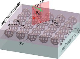
Fig. 5.16: Configuration of the studied cases.

For the four selected cases, among six found in the literature, published results are compared to ones given by our formulation of the FEM. Moreover, in each case, a satisfying global energy balance is detailed. Finally a new validation case combining all the difficulties encountered when modeling crossed-gratings is proposed: A non-trivial geometry for the diffractive pattern (a torus), made of an arbitrary lossy material leading to a large step of index and illuminated by a plane wave with an oblique incidence. Convergence of the FEM calculation as well as computation time will be discussed in Sec. 5.3.4.

Checkerboard grating

In this example worked out by L. Li [27], the diffractive element is a rectangular parallelepiped as shown Fig. 5.17a and the grating parameter highlighted in Fig. 5.16 are the following: $\varphi_{0}=\theta_{0}=0^{\,\circ}$, $\psi_{0}=45^{\,\circ}$, $d_{x}=d_{y}=5\,\lambda_{0}\,\sqrt{2}/4$, $h=\lambda_{0}$, $\varepsilon^{+}=\varepsilon^{g^{\prime}}=2.25$ and $\varepsilon^{-}=\varepsilon^{g}=1$.

(a)

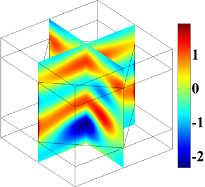
(b)

Fig. 5.17: Diffractive element with vertical edges (a). $\Re{\it{e}}\{E_{x}\}$ in V/m (b).

	FMM [27]	FEM
$T_{-1,-1}$	0.04308	0.04333
$T_{-1,0}$	0.12860	0.12845
$T_{-1,+1}$	0.06196	0.06176
$T_{0,-1}$	0.12860	0.12838
$T_{0,0}$	0.17486	0.17577
$T_{0,+1}$	0.12860	0.12839
$T_{+1,-1}$	0.06196	0.06177
$T_{+1,0}$	0.12860	0.12843
$T_{+1,+1}$	0.04308	0.04332
${\color[rgb]{0,0,0}\displaystyle\sum_{(n,m)\in\mathbb{Z}}}\Re{\it{e}}\{R_{n,m}\}$	-	0.10040
TOTAL	-	1.00000

Tab. 5.4: Energy balance [27].

Our formulation of the FEM shows good agreement with the Fourier Modal Method developed by L. Li ([27], 1997) since the maximal relative difference between the array of values presented in Table 5.4 remains lower than $\textrm{10}^{\textrm{-3}}$. Moreover, the sum of the efficiencies of propagative orders given by the FEM is very close to 1 in spite of the addition of all errors of determination upon the efficiencies.

Pyramidal crossed-grating

In this example firstly worked out by Derrick et al. [39], the diffractive element is a pyramid with rectangular basis as shown Fig. 5.18a and the grating parameters highlighted in Fig. 5.16 are the following: $\lambda_{0}=1.533$, $\varphi_{0}=45^{\,\circ}$, $\theta_{0}=30^{\,\circ}$, $\psi_{0}=0^{\,\circ}$, $d_{x}=1.5$, $d_{y}=1$, $h=0.25$, $\varepsilon^{+}=\varepsilon^{g}=1$ and $\varepsilon^{-}=\varepsilon^{g^{\prime}}=2.25$.

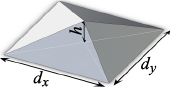
(a)

(b)

Fig. 5.18: Diffractive element with oblique edges (a). $\Re{\it{e}}\{E_{y}\}$ in V/m (b).

Given in	[39]	[40]	[41]	[42]	FEM
$R_{-1,0}$	0.00254	0.00207	0.00246	0.00249	0.00251
$R_{0,0}$	0.01984	0.01928	0.01951	0.01963	0.01938
$T_{-1,-1}$	0.00092	0.00081	0.00086	0.00086	0.00087
$T_{0,-1}$	0.00704	0.00767	0.00679	0.00677	0.00692
$T_{-1,0}$	0.00303	0.00370	0.00294	0.00294	0.00299
$T_{0,0}$	0.96219	0.96316	0.96472	0.96448	0.96447
$T_{1,0}$	0.00299	0.00332	0.00280	0.00282	0.00290
TOTAL	0.99855	1.00001	1.00008	0.99999	1.00004

Tab. 5.5: Comparison with the results given in [39, 40, 41, 42].

Results given by the FEM show good agreement with ones of the C method [39, 42], the Rayleigh method [40] and the RCWA [41]. Note that, in this case, some edges of the diffractive element are oblique.

Bi-sinusoidal grating

In this example worked out by Bruno et al. [43], the surface of the grating is bi-sinusoidal (see Fig. 5.19a) and described by the function $f$ defined by:

$$f(x,y)=\frac{h}{4}\left[\cos\left(\frac{2\,\pi\,x}{d}\right)+\cos\left(\frac{2\,\pi\,y}{d}\right)\right]$$ (5.79)

The grating parameters et al.highlighted in Fig. 5.16 are the following: $\lambda_{0}=0.83$, $\varphi_{0}=\theta_{0}=\psi_{0}=0^{\,\circ}$, $d_{x}=d_{y}=1$, $h=0.2$, $\varepsilon^{+}=\varepsilon^{g}=1$ and $\varepsilon^{-}=\varepsilon^{g^{\prime}}=4$.

(a)

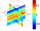
(b)

Fig. 5.19: Diffractive element with oblique edges (a). $\Re{\it{e}}\{E_{z}\}$ in V/m (b).

	[43]	FEM
$R_{-1,0}$	0.01044	0.01164
$R_{0,-1}$	0.01183	0.01165
$T_{-1,-1}$	0.06175	0.06299
${\color[rgb]{0,0,0}\displaystyle\sum_{(n,m)\in\mathbb{Z}}}\Re{\it{e}}\{R_{n,m}\}$	-	0.10685
${\color[rgb]{0,0,0}\displaystyle\sum_{(n,m)\in\mathbb{Z}}}\Re{\it{e}}\{T_{n,m}\}$	-	0.89121
TOTAL	-	0.99806

Tab. 5.6: Energy balance [43].

Note that in order to define this surface, the bi-sinusoid was first sampled ($15\times 15$ points), then converted to a 3D file format. This sampling can account for the slight differences with the results obtained using the method of variation of boundaries developed by Bruno et al. (1993).

Circular apertures in a lossy layer

In this example worked out by Schuster et al. [44], the diffractive element is a circular aperture in a lossy layer as shown Fig. 5.20a and the grating parameter highlighted in Fig. 5.16 are the following: $\lambda_{0}=500\,$nm, $\varphi_{0}=\theta_{0}=0^{\,\circ}$, $\varepsilon^{+}=\varepsilon^{g}=1$, $\varepsilon^{g^{\prime}}=0.8125+5.2500\,i$ and $\varepsilon^{-}=2.25$.

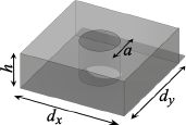
(a)

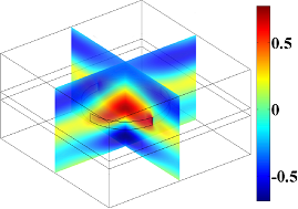
(b)

Fig. 5.20: Lossy diffractive element with vertical edges (a). $\Re{\it{e}}\{E_{y}\}$ in V/m (b).

	[45]	[27]	[44]	FEM
$R_{0,0}$	0.24657	0.24339	0.24420	0.24415
${\color[rgb]{0,0,0}\displaystyle\sum_{(n,m)\in\mathbb{Z}}}\Re{\it{e}}\{T_{n,m}\}$	$-$	$-$	$-$	0.29110
${\color[rgb]{0,0,0}\displaystyle\sum_{(n,m)\in\mathbb{Z}}}\Re{\it{e}}\{R_{n,m}\}$	$-$	$-$	$-$	0.26761
$Q$	$-$	$-$	$-$	0.44148
TOTAL	$-$	$-$	$-$	1.00019

Tab. 5.7: Comparison with [45, 27, 44] and energy balance.

In this lossy case, results obtained with the FEM show good agreement with the ones obtained with the FMM [27], the differential method [44, 46] and the RCWA [45]. Joule losses inside the diffractive element can be easily calculated, which allows to provide a global energy balance for this configuration. Finally, the convergence of the value $R_{0,0}$ as a function of the mesh refinement will be examined.

Lossy tori grating

We finally propose a new test case for crossed-grating numerical methods. The major difficulty of this case lies both in the non trivial geometry (see Fig. 5.21a) of the diffractive object and in the fact that it is made of a material chosen so that losses are optimal inside it. The grating parameters highlighted in Fig. 5.16 and Fig. 5.21a are the following: $\lambda_{0}=1$, $\varphi_{0}=\psi_{0}=0^{\,\circ}$, $d_{x}=d_{y}=0.3\,$, $a=0.1$, $b=0.05$, $R=0.15$, $h=500\,$nm, $\varepsilon^{+}=\varepsilon^{g}=1$, $\varepsilon^{g^{\prime}}=-21+20\,i$ and $\varepsilon^{-}=2.25$.

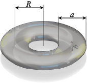
(a)

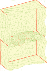
(b)

Fig. 5.21: Torus parameters (a). Coarse mesh of the computational domain (b).

FEM 3D	$\theta=0^{\circ}$	$\theta=40^{\circ}$
$R_{0,0}$	0.36376	0.27331
$T_{0,0}$	0.32992	0.38191
$Q$	0.30639	0.34476
TOTAL	1.00007	0.99998

Tab. 5.8: Energy balances at normal and oblique incidence.

Tab. 5.8 illustrates the independence of our method towards the geometry of the diffractive element. $\varepsilon^{g^{\prime}}$ is chosen so that the skin depth has the same order of magnitude as $b$, which maximizes losses. Note that energy balances remain very accurate at normal and oblique incidence, in spite of both the non-triviality of the geometry and the strong losses.

Convergence and computation time

Convergence as a function of mesh refinement

When using modal methods such as the RCWA or the differential method, based on the calculation of Rayleigh coefficients, a number proportional to $N_{R}$ have to be be determined a priori. Then, the unknown diffracted field is expanded as a Fourier serie, injected under this form in Maxwell equations, which annihilates $x-$ and $y-$dependencies. This leads to a system of coupled partial differential equations whose coefficients can structured in a matrix formalism. The resulting matrix is sometimes directly invertible (RCWA) depending on whether the geometry allows to suppress the $z-$dependance, which makes this method adapted to diffractive elements with vertically (or decomposed in staircase functions) shaped edge. In some other cases, one has to make the use of integral methods in order to solve the system, as in the pyramidal case for instance, which leads to the so-called differential method. The diffracted field map can be deduced from these coefficients. If the grating configuration only calls for a few propagative orders and if the field inside the groove region is not the main information sought for, these two close methods allow to determine the repartition of the incident energy quickly. However, if the field inside the groove region is the main piece of information, it is advisable to calculate many Rayleigh coefficients corresponding to evanescent waves which increases the computation time as $(N_{R})^{3}$ or even $(N_{R})^{4}$.

FEM relies on the direct calculation of the vectorial components of the complex field. Rayleigh coefficients are determined a posteriori. The parameter limiting the computation time is the number of tetrahedral elements along which the computational domain is split up. We suppose that it is necessary to calculate at least two or three points (or mesh nodes) per period of the field ($\lambda_{0}/\sqrt{\Re{\it{e}}\{\varepsilon\}}$). Figure 5.22 shows the convergence of the efficiency $R_{0,0}$ (circular apertures case, see Fig. 5.20a) as a function of the mesh refinement characterized by the parameter $N_{M}$: The maximum size of each element is set to $\lambda_{0}/(N_{M}\,\sqrt{\Re{\it{e}}\{\varepsilon\}})$.

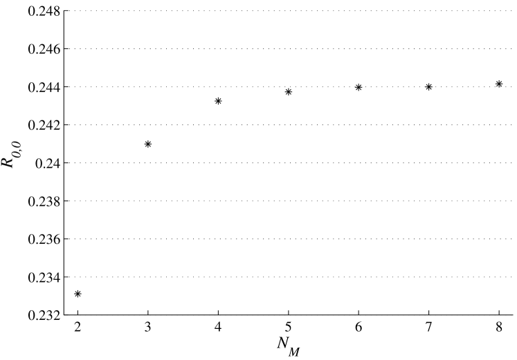
Fig. 5.22: Convergence of $R_{0,0}$ in function of $N_{m}$ (circular apertures crossed-grating).

It is of interest to note that even if $N_{M}<3$ the FEM still gives pertinent diffraction efficiencies: $R_{0,0}=\textrm{0.2334}$ for $N_{M}=\textrm{1}$ and $R_{0,0}=\textrm{0.2331}$ for $N_{M}=\textrm{2}$. The Galerkin method (see Eq. (5.67)) corresponds to a minimization of the error (between the exact solution and the approximation) with respect to a norm that can be physically interpreted in terms of energy-related quantities. Therefore, the finite element methods usually provide energy-related quantities that are more accurate than the local values of the fields themselves.

Computation time

All the calculations were performed on a server equipped with 8 dual core Itanium1 processors and 256Go of RAM. Tetrahedral quadratic edge elements were used together with the direct solver PARDISO. Among different direct solvers adapted to sparse matrix algebra (UMFPACK, SPOOLES and PARDISO), PARDISO turned out to be the less time-consuming one as shown in Tab 5.9.

Solver	Computation time for 41720 DOF	Computation time for 205198 DOF
SPOOLES	$15\,$mn$\,32\,$s	$14\,$h$44\,$mn
UMFPACK	$2\,$mn$\,07\,$s	$1\,$h$12\,$mn
PARDISO	$57\,$s	$16\,$mn

Tab. 5.9: Computation time variations from solver to solver.

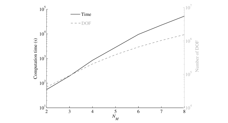
Fig. 5.23: Computation time and number of DOF as a function of $N_{M}$.

Figure 5.23 shows the computation time required to perform the whole FEM computational process for a system made of a number of DOF indicated on the right-hand ordinate. It is of importance to note that for values of $N_{M}$ lower than 3, the problem can be solved in less than a minute on a standard laptop (4Go RAM, $2\times 2\,$GHz) with 3 significant digits on the diffraction efficiencies. This accuracy is more than sufficient in numerous experimental cases. Furthermore, as far as integrated values are at stake, relatively coarse meshes ($N_{M}\approx 1$) can be used trustfully, authorizing fast geometric, spectral or polarization studies.

Nowadays, the efficiency of the numerical algorithms for sparse matrix algebra together with the available power of computers and the fact that the problem reduces to a basic cell with a size of a small number of wavelengths make the finite element problem very tractable as proved here.

5.4 Concluding remarks

In this chapter, we demonstrate a general formulation of the FEM allowing to calculate the diffraction efficiencies from the electromagnetic field diffracted by arbitrarily shaped gratings embedded in a multilayered stack lightened by a plane wave of arbitrary incidence and polarization angle. It relies on a rigorous treatment of the plane wave sources problem through an equivalent radiation problem with localized sources. Bloch conditions and a new dedicated PML have been implemented in order to rigorously truncate the computational domain.

The principles of the method were discussed in detail for mono-dimensional gratings in TE/TM polarization cases (2D or scalar case) in a first part, and for the most general bi-dimensional or crossed gratings (3D or vector case) in a second part. Note that the very same concepts could be applied to the intermediate case of mono-dimensional gratings enlighten by an arbitrary incident plane wave (so-called conical case). The reader will find detail about the element basis relevant to this case in [11].

The main advantage of this formulation is its complete generality with respect to the studied geometries and the material properties, as illustrated with the lossy tori grating non-trivial case. Its principle remains independent of both the number of diffractive elements by period and number of stack layers. Its flexibility allowed us to retrieve with accuracy the few numerical academic examples found in the literature and established with independent methods.

The remarkable accuracy observed in the case of coarse meshes, makes it a fast tool for the design and optimization of diffractive optical components (e.g. reflection and transmission filters, polarizers, beam shapers, pulse compression gratings…). The complete independence of the presented approach towards both the geometry and the isotropic constituent materials of the diffractive elements makes it a handy and powerful tool for the study of metamaterials, finite-size photonic crystals, periodic plasmonic structures…The method described in this chapter has already been successfully applied to various problems, from homogenization theory [47] or transformation optics [48] to more applied concerns as the modeling of complex CMOS nanophotonic devices [49] or ultra-thin new generation solar cells [50].

5.A APPENDIX

This appendix is dedicated to the determination of the vector electric field in a dielectric stack enlightened by a plane wave of arbitrary polarization and incidence angle. This calculation, abundantly treated in the 2D scalar case, is generally not presented in the literature since, as far as isotropic cases are concerned, it is possible to project the general vectorial case on the two reference TE and TM cases. However, the presented formulation can be extended to a fully anisotropic case for which this TE/TM decoupling is no longer valid and the three components of the field have to be calculated as follows.

Let us consider the ancillary problem mentioned in Sec. 5.3.2, i.e. a dielectric stack made of $N$ homogeneous, isotropic, lossy layers characterized by there relative permittivity denoted $\varepsilon^{j}$ and their thickness $e_{j}$. This stack is deposited on a homogeneous, isotropic, possibly lossy substrate characterized by its relative permittivity denoted $\varepsilon^{N+1}=\varepsilon^{-}$. The superstrate is air and its relative permittivity is denoted $\varepsilon^{+}=1$. Finally, we denote by $z_{j}$ the altitude of the interface between the $j^{th}$ and $j+1^{th}$ layers. The restriction of the incident field $\mathbf{E}^{\mathrm{inc}}$ to the superstrate region is denoted $\mathbf{E}_{0}$. The problem amounts to looking for ($\mathbf{E}_{1}$,$\mathbf{H}_{1}$) satisfying Maxwell equations in harmonic regime (see Eqs. (5.56a,5.56b)).

Across the interface $z=z_{j}$

By projection on the main axis of the vectorial Helmholtz propagation equation (Eq. (5.57)), the total electric field inside the $j^{th}$ layer can be written as the sum of a propagative and a counter-propagative plane waves:

$$\mathbf{E}_{1}(x,y,z)=\left[\begin{array}[]{l}E_{1}^{x,j,+}\\ E_{1}^{y,j,+}\\ E_{1}^{z,j,+}\end{array}\right]\exp\left(j\,(\alpha_{0}\,x+\beta_{0}\,y+\gamma_{j}\,z)\right)+\left[\begin{array}[]{l}E_{1}^{x,j,-}\\ E_{1}^{y,j,-}\\ E_{1}^{z,j,-}\end{array}\right]\exp\left(j\,(\alpha_{0}\,x+\beta_{0}\,y-\gamma_{j}\,z)\right)$$ (5.80)

where

$$\gamma_{j}^{2}=k_{j}^{2}-\alpha_{0}^{2}-\beta_{0}^{2}$$ (5.81)

What follows consists in writing the continuity of the tangential components of $(\mathbf{E}_{1},\mathbf{H}_{1})$ across the interface $z=z_{j}$, i.e. the continuity of the vector field $\Psi$ defined by:

$$\Psi=\left[\begin{array}[]{l}E_{1}^{x}\\ E_{1}^{y}\\ i\,H_{1}^{x}\\ i\,H_{1}^{y}\end{array}\right].$$ (5.82)

The continuity of $\Psi$ along $Oz$ together with its analytical expression inside the $j^{th}$ and $j+1^{th}$ layers allows to establish a recurrence relation for the interface $z=z_{j}$.

Then, by projection of Eqs. (5.56a,5.56b) on $Ox$,$Oy$ and $Oz$:

$$\left[\begin{array}[]{l}i\,\beta_{0}\,H_{1}^{z}-\frac{\partial H_{1}^{y}}{dz}\\ \frac{\partial H_{1}^{x}}{dz}-i\,\alpha_{0}\,H_{1}^{z}\\ i\,\alpha_{0}\,H_{1}^{y}-i\,\beta_{0}\,H_{1}^{x}\end{array}\right]=-i\,\omega\,\varepsilon\left[\begin{array}[]{l}E_{1}^{x}\\ E_{1}^{y}\\ E_{1}^{z}\end{array}\right]$$ (5.83)

and

$$\left[\begin{array}[]{l}i\,\beta_{0}\,E_{1}^{z}-\frac{\partial E_{1}^{y}}{\partial z}\\ \frac{\partial E_{1}^{x}}{\partial z}-i\,\alpha_{0}\,E_{1}^{z}\\ i\,\alpha_{0}\,E_{1}^{y}-i\,\beta_{0}\,E_{1}^{x}\end{array}\right]=i\,\omega\,\mu\left[\begin{array}[]{l}H_{1}^{x}\\ H_{1}^{y}\\ H_{1}^{z}\end{array}\right].$$ (5.84)

Consequently, tangential components of $\mathbf{H}_{1}$ can be expressed in function of tangential components of $\mathbf{E}_{1}$:

$$\underbrace{\begin{bmatrix}\omega\,\mu&0&\beta_{0}\\ 0&\omega\,\mu&-\alpha_{0}\\ -\beta_{0}&\alpha_{0}&-\omega\,\varepsilon\end{bmatrix}\,}_{B}\begin{bmatrix}i\,H_{1}^{x}\\ i\,H_{1}^{y}\\ i\,H_{1}^{z}\end{bmatrix}=\begin{bmatrix}\frac{\partial E_{1}^{y}}{dz}\\ -\frac{\partial E_{1}^{x}}{dz}\\ 0\end{bmatrix}.$$ (5.85)

By noticing the invariance and linearity of the problem along $Ox$ and $Oy$, the following notations are adopted:

$$\left\{\begin{array}[]{l}U_{x}^{j,\pm}=E_{1}^{x,j,\pm}\,\exp(\pm\,i\,\gamma_{j}\,z)\\ U_{y}^{j,\pm}=E_{1}^{y,j,\pm}\,\exp(\pm\,i\,\gamma_{j}\,z)\end{array}\right.$$ (5.86)

and

$$\Phi_{j}=\left[\begin{array}[]{l}U_{x}^{+,j}\\ U_{x}^{-,j}\\ U_{y}^{+,j}\\ U_{y}^{-,j}\end{array}\right].$$ (5.87)

Thanks to Eq. (5.80) and Eq. (5.84) and letting $M=B^{-1}$, it comes for the $j^{th}$ layer:

$$\Psi(x,y,z)=\exp(i(\alpha_{0}\,x+\beta_{0}\,y))\,\underbrace{\begin{bmatrix}1&1&0&0\\ 0&0&1&1\\ \gamma_{j}\,M^{j}_{12}&-\gamma_{j}\,M^{j}_{12}&-\gamma_{j}\,M^{j}_{11}&\gamma_{j}\,M^{j}_{11}\\ \gamma_{j}\,M^{j}_{22}&-\gamma_{j}\,M^{j}_{22}&-\gamma_{j}\,M^{j}_{21}&\gamma_{j}\,M^{j}_{21}\\ \end{bmatrix}}_{\Pi_{j}}\,\left[\begin{array}[]{l}U_{x}^{+,j}\\ U_{x}^{-,j}\\ U_{y}^{+,j}\\ U_{y}^{-,j}\end{array}\right].$$ (5.88)

Finally, the continuity of $\Psi$ at the interface $z=z_{j}$ leads to:

$$\Phi_{j+1}(z_{j})=\Pi_{j+1}^{-1}\,\Pi_{j}\,\Phi_{j}(z_{j}).$$ (5.89)

Normal components can be deduced using Eqs. (5.83,5.84).

Traveling inside the $j+1^{th}$ layer

Using Eq. (5.80), a simple phase shift allows to travel from $z=z_{j}$ to $z=z_{j+1}=z_{j}-e_{j+1}$:

$$\Phi_{j+1}(z_{j+1})=\underbrace{\begin{bmatrix}\exp(-i\,\gamma_{j+1}\,e_{j+1})&0&0&0\\ 0&\exp(+i\,\gamma_{j+1}\,e_{j+1})&0&0\\ 0&0&\exp(-i\,\gamma_{j+1}\,e_{j+1})&0\\ 0&0&0&\exp(+i\,\gamma_{j+1}\,e_{j+1})\\ \end{bmatrix}}_{T_{j+1}}\,\Phi_{j+1}(z_{j})$$ (5.90)

Thanks to Eq. (5.90) and Eq. (5.89), a recurrence relation can be formulated for the analytical expression of $\mathbf{E}_{1}$ in each layer:

$$\Phi_{j+1}(z_{j+1})=T_{j+1}\,\Pi_{j+1}^{-1}\,\Pi_{j}\,\Phi_{j}(z_{j})$$ (5.91)

Reflection and transmission coefficients

The last step consists in the determination of the first term $\Phi_{0}$, which is not entirely known, since the problem definition only specifies $U_{x}^{0,+}$ and $U_{y}^{0,+}$, imposed by the incident field $\mathbf{E}_{0}$. Let us make the use of the OWC hypothesis verified by $\mathbf{E}_{1}^{d}$ (see Eq. (5.62)). This hypothesis directly translates the fact that none of the components of $\mathbf{E}_{1}^{d}$ can either be traveling down in the superstrate or up in the substrate: $U_{y}^{N+1,-}=U_{x}^{N+1,-}=0$. Therefore, the four unknowns $U_{x}^{0,-}$, $U_{y}^{0,-}$,$U_{y}^{N+1,+}$ and $U_{x}^{N+1,+}$, i.e. transverse components of the vector fields reflected and transmitted by the stack, verify the following equation system:

$$\Phi_{N+1}(z_{N})=(\Pi_{N+1})^{-1}\,\Pi_{N}\prod_{j=0}^{N-1}T_{N-j}\,(\Pi_{N-j})^{-1}\,\Pi_{N-j-1}\,\Phi_{0}(z_{0})$$ (5.92)

This allows to extend the definition of transmission and reflection widely used in the scalar case. Finally, $\Phi_{N+1}$ is entirely defined. Making the use of the recurrence relation of Eq. (5.91) and of Eq. (5.80) leads to an analytical expression for $\mathbf{E}_{1}^{d}$ in each layer.

References:

- [1] A. Bossavit, “Solving Maxwell equations in a closed cavity, and the question ofspurious modes,” IEEE Trans. on Mag. 26, 702–705 (1990).
- [2] J-C. Nedelec, “Mixed finite elements in R 3,” Numerische Mathematik 35, 315–341 (1980).
- [3] A. Bossavit, “Solving maxwell equations in a closed cavity, and the question ofspurious modes’,” Magnetics, IEEE Transactions on 26, 702–705 (1990).
- [4] J-P. Berenger, “A perfectly matched layer for the absorption of electromagnetic waves,” J. Comput. Phys. 114, 185–200 (1994).
- [5] W. Chew and W. Weedon, “A 3d perfectly matched medium from modified maxwell’s equations with stretched coordinates,” Microwave and optical technology letters 7, 599–604 (2007).
- [6] F. Teixeira and W. Chew, “General closed-form pml constitutive tensors to match arbitrary bianisotropic and dispersive linear media,” Microwave and Guided Wave Letters, IEEE 8, 223–225 (1998).
- [7] A. Nicolet, F. Zolla, Y. Agha, and S. Guenneau, “Geometrical transformations and equivalent materials in computational electromagnetism,” COMPEL 27, 806–819 (2008).
- [8] Y. Agha, F. Zolla, A. Nicolet, and S. Guenneau, “On the use of pml for the computation of leaky modes: An application to microstructured optical fibres,” COMPEL 27, 95–109 (2008).
- [9] R. Petit, L. Botten et al., Electromagnetic theory of gratings, vol. 62 (Springer-Verlag Berlin, 1980).
- [10] F. Zolla, G. Renversez, and A. Nicolet, Foundations of Photonic Crystal Fibres: 2nd Edition (Imperial College Press, 2012).
- [11] A. Nicolet, S. Guenneau, C. Geuzaine and F. Zolla, “Modelling of electromagnetic waves in periodic media with finite elements,” J. of Comput. and Applied Math. 168, 321–329 (2004).
- [12] A. Nicolet, F. Zolla, Y. Ould Agha and S. Guenneau, “Leaky modes in twisted microstructured optical fibres,” Waves in Random and Complex Media 17, 559–570 (2007).
- [13] M. Lassas, J. Liukkonen and E. Somersalo, “Complex riemannian metric and absorbing boundary condition,” Journal de Mathématiques Pures et Appliquées 80, 739–768 (2001).
- [14] J. L. M. Lassas and E. Somersalo, “Analysis of the PML equations in general convex geometry,” Proceedings of the Royal Society of Edinburgh 131, 1183–1207 (2001).
- [15] A. Nicolet, F. Zolla, Y. O. Agha, and S. Guenneau, “Geometrical transformations and equivalent materials in computational electromagnetism,” COMPEL 27, 806–819 (2008).
- [16] P. Helluy, S. Maire and P. Ravel, “Intégrations numériques d’ordre élevé de fonctions régulières ou singulières sur un intervalle,” CR. Acad. Sci. Paris, Sér. I, Math 327, 843–848 (1998).
- [17] G. Granet, “Reformulation of the lamellar grating problem through the concept of adaptive spatial resolution,” J. Opt. Soc. Am. A 16, 2510–2516 (1999).
- [18] G. Bao, Z. Chen and H. Wu, “Adaptive finite-element method for diffraction gratings,” J. Opt. Soc. Am. A 22, 1106–1114 (2005).
- [19] G. Tayeb., Contribution à l’étude de la diffraction des ondes électromagnétiques par des réseaux. Réflexions sur les méthodes existantes et sur leur extension aux milieux anisotropes. (Thèse de doctorat en sciences (PhD), Université Aix-Marseille III, 1990).
- [20] Y. Ohkawa, Y. Tsuji and M. Koshiba, “Analysis of anisotropic dielectric grating diffraction using the finite-element method,” J. Opt. Soc. Am. A 13, 1006–1012 (1996).
- [21] N. Kono and Y. Tsuji, “A novel finite-element method for nonreciprocal magneto-photonic crystal waveguides,” Journal of lightwave technology 22, 1741 (2004).
- [22] A. Zhou, J. Erwin, C. Brucker, and M. Mansuripur, “Dielectric tensor characterization for magneto-optical recording media,” Applied optics 31, 6280–6286 (1992).
- [23] R. W. Wood, “On a Remarkable Case of Uneven Distribution of Light in a Diffraction Grating Spectrum,” Proceedings of the Physical Society of London 18, 269–275 (1902).
- [24] L. Rayleigh, “Note on the remarkable case of diffraction spectra described by Prof. Wood,” Philos. Mag 14, 60–65 (1907).
- [25] Z. Chen and X. Liu, “An adaptive perfectly matched layer technique for time-harmonic scattering problems,” SIAM J. Numer. Anal. 43, 645–671 (2005).
- [26] A. Schädle, L. Zschiedrich, S. Burger, R. Klose, and F. Schmidt, “Domain decomposition method for maxwell’s equations: Scattering off periodic structures,” Journal of Computational Physics 226, 477–493 (2007).
- [27] L. Li, “New formulation of the fourier modal method for crossed surface-relief gratings,” J. Opt. Soc. Am. A 14, 2758–2767 (1997).
- [28] E. Popov, M. Nevière, B. Gralak and G. Tayeb, “Staircase approximation validity for arbitrary-shaped gratings,” J. Opt. Soc. Am. A 19, 33–42 (2002).
- [29] G. Demésy, F. Zolla, A. Nicolet, M. Commandré and C. Fossati, “The finite element method as applied to the diffraction by an anisotropic grating,” Optics Express 15, 18089–18102 (2007).
- [30] G. Demésy, F. Zolla, A. Nicolet, M. Commandré, C. Fossati, O. Gagliano, S. Ricq and B. Dunne, “Finite element method as applied to the study of gratings embedded in complementary metal-oxide semiconductor image sensors,” Optical Engineering 48, 058002 (2009).
- [31] F. Zolla and R. Petit, “Method of fictitious sources as applied to the electromagnetic diffraction of a plane wave by a grating in conical diffraction mounts,” J. Opt. Soc. Am. A 13, 796–802 (1996).
- [32] Y. Ould Agha, F. Zolla, A. Nicolet and S. Guenneau, “On the use of PML for the computation of leaky modes : an application to gradient index MOF,” COMPEL 27, 95–109 (2008).
- [33] P. Dular, A. Nicolet, A. Genon and W. Legros, “A discrete sequence associated with mixed finite elements and itsgauge condition for vector potentials,” IEEE Transactions on Magnetics 31, 1356–1359 (1995).
- [34] P. Ingelstrom, “A new set of H (curl)-conforming hierarchical basis functions for tetrahedral meshes,” IEEE Trans. Microwave Theory Tech. 54, 106–114 (2006).
- [35] A. Bossavit and I. Mayergoyz, “Edge-elements for scattering problems,” IEEE Trans. on Mag. 25, 2816–2821 (1989).
- [36] T. V. Yioultsis and T. D. Tsiboukis, “The Mystery and Magic of Whitney Elements - An Insight in their Properties and Construction,” ICS Newsletter 3, 1389–1392 (Nov. 1996).
- [37] T. V. Yioultsis and T. D. Tsiboukis, “Multiparametric vector finite elements: a systematic approach to the construction of three-dimensional, higher order, tangential vector shape functions,” IEEE Trans. on Mag. 32, 1389–1392 (1996).
- [38] E. Noponen and J. Turunen, “Eigenmode method for electromagnetic synthesis of diffractive elements with three-dimensional profiles,” J. Opt. Soc. Am. A 11, 2494–2502 (1994).
- [39] G. H. Derrick, R. C. McPhedran, D. Maystre and M. Nevière, “Crossed gratings: A theory and its applications,” Appl. Phys. B 18, 39–52 (1979).
- [40] J. J. Greffet, C. Baylard and P. Versaevel, “Diffraction of electromagnetic waves by crossed gratings: a series solution,” Opt. Lett. 17, 1740–1742 (1992).
- [41] R. Bräuer and O. Bryngdahl, “Electromagnetic diffraction analysis of two-dimensional gratings,” Opt. Commun. 100 (1993).
- [42] G. Granet, “Analysis of diffraction by surface-relief crossed gratings with use of the Chandezon method: Application to multilayer crossed gratings,” J. Opt. Soc. Am. A 15, 1121–1131 (1998).
- [43] O. P. Bruno and F. Reitich, “Numerical solution of diffraction problems: a method of variation of boundaries. III. doubly periodic gratings,” J. Opt. Soc. Am. A 10, 2551–2562 (1993).
- [44] T. Schuster, J. Ruoff, N. Kerwien, S. Rafler and W. Osten, “Normal vector method for convergence improvement using the rcwa for crossed gratings,” J. Opt. Soc. Am. A 24, 2880–2890 (2007).
- [45] M. G. Moharam, E. B. Grann, D. A. Pommet and T. K. Gaylord, “Formulation for stable and efficient implementation of the rigorous coupled-wave analysis of binary gratings,” J. Opt. Soc. Am. A 12, 1068–1076 (1995).
- [46] L. Arnaud, Diffraction et diffusion de la lumière : modélisation tridimensionnelle et application à la métrologie de la microélectronique et aux techniques d’imagerie sélective en milieu diffusant (PhD Thesis, Université Aix-Marseille III, 2008).
- [47] A. Cabuz, A. Nicolet, F. Zolla, D. Felbacq, and G. Bouchitté, “Homogenization of nonlocal wire metamaterial via a renormalization approach,” J. Opt. Soc. Am. B 28, 1275–1282 (2011).
- [48] G. Dupont, S. Guenneau, S. Enoch, G. Demesy, A. Nicolet, F. Zolla, and A. Diatta, “Revolution analysis of three-dimensional arbitrary cloaks,” Optics Express 17, 22603–22608 (2009).
- [49] G. Demésy, F. Zolla, A. Nicolet, M. Commandré, C. Fossati, O. Gagliano, S. Ricq, and B. Dunne, “Finite element method as applied to the study of gratings embedded in complementary metal-oxide semiconductor image sensors,” Optical Engineering 48, 058002–058002 (2009).
- [50] G. Demésy and S. John, “Solar energy trapping with modulated silicon nanowire photonic crystals,” Journal of Applied Physics 112, 074326–074326 (2012).