A Comparison of Relaxations of Multiset Cannonical Correlation Analysis and Applications

Abstract

Canonical correlation analysis is a statistical technique that is used to find relations between two sets of variables. An important extension in pattern analysis is to consider more than two sets of variables. This problem can be expressed as a quadratically constrained quadratic program (QCQP), commonly referred to Multi-set Canonical Correlation Analysis (MCCA). This is a non-convex problem and so greedy algorithms converge to local optima without any guarantees on global optimality. In this paper, we show that despite being highly structured, finding the optimal solution is NP-Hard. This motivates our relaxation of the QCQP to a semidefinite program (SDP). The SDP is convex, can be solved reasonably efficiently and comes with both absolute and output-sensitive approximation quality. In addition to theoretical guarantees, we do an extensive comparison of the QCQP method and the SDP relaxation on a variety of synthetic and real world data. Finally, we present two useful extensions: we incorporate kernel methods and computing multiple sets of canonical vectors.

1 Introduction

Natural phenomena are often the product of several factors interacting. A fundamental challenge of pattern analysis and machine learning is to find the relationships between these factors. Real world datasets are often modeled using distributions such as mixtures of Gaussians. These models often capture the uncertainty inherent in both underlying systems and measurements. Canonical correlation analysis (CCA) is a well-known statistical technique developed to find the relationships between two sets of random variables. The relations or patterns discovered by CCA can be used in two ways. First, they can be used to obtain a common representation for both sets of variables. Second, the patterns themselves can be used in an exploratory analysis (see [11] for example).

It is possible to extend this idea beyond two sets. The problem is then known as the Multi-set Canonical Correlation Analysis (MCCA). Whereas it can be shown that CCA can be solved using an (generalized) eigenvalue computation, MCCA is a much more difficult problem. One approach is to express it as a non-convex quadratically constrained quadratic program (QCQP). In this paper, we show that despite being a highly structured problem, it is NP-hard. We then describe an efficient algorithm for finding a locally optimal solutions to the problem.

Since the algorithm is local and the problem non-convex, we cannot guarantee the quality of the solutions obtained. Therefore, we give a relaxation of the problem based on semi-definite programming (SDP) which gives a constant factor approximation as well as an output sensitive guarantee.

For use in practical applications, we describe two important extensions: we adapt the methods to use kernels and to find multi-dimensional solutions.

Finally, we perform extensive experimentation to compare the efficient local algorithm and the SDP relaxation on both synthetic and real-world datasets. Here, we show experimentally that the hardness of the problem is in some sense generic in low dimensions. That is, a randomly generated problem in low dimensions will result in many local maxima which are far from the global optimum. Somewhat surprisingly, this does not occur in higher dimensions.

Our contributions in this paper are as follows:

• We show that in general MCCA is NP-hard.

• We describe an scalable and efficient algorithm for finding a locally optimal solution.

• Using an SDP relaxation of the problem, we can compute a global upper bound on the objective function along with various approximation guarantees on solutions based on this relaxations.

• We describe two extensions which are important for practical applications: a kernel method and computing multiple sets of canonical vectors.

• An extensive experimental evaluation of the respective algorithms: we show that in practice the local algorithm performs extremely well, something we can verify with using the SDP relaxation as well as show there are cases where the local algorithm is far from the optimal solution. We do this with a combination of synthetic and real world examples.

• We propose a preprocessing step based on random projections, which enables us to apply the SDP bounds on large, high dimensional data sets.

The paper is organized as following. Section 2 describes the background and related work. Section 3 introduces the main optimization problem, discusses the problem complexity and presents several bounds on optimal solutions. Section 4 describes the extensions of the original formulation to higher-dimensional, nonlinear case. Section 5 presents empirical work based on synthetic and real data. Conclusions and future work is discussed in section 6. Finally, in the Appendix we included a primer for the notation used in the paper.

2 Background

Canonical Correlation Analysis (CCA), introduced by Harold Hotelling [16], was developed to detect linear relations between two sets of variables. Typical uses of CCA include statistical tests of dependence between two random vectors, exploratory analysis on multi-view data, dimensionality reduction and finding a common embedding of two random vectors that share mutual information.

CCA has been generalized in two directions: extending the method to finding nonlinear relations by using kernel methods [17][12] (see [27] for an introduction to kernel methods) and extending the method to more than two sets of variables which was introduced in [18]. Among several proposed generalizations in [18] the most notable is the sum of correlations (SUMCOR) generalization and it is the focus of our paper. There the result is to project $m$ sets of random variables to $m$ univariate random variables, which are pair-wise highly correlated on average. An iterative method to solve the SUMCOR generalization was proposed in [15] and the proof of convergence was established in [2]. In [2] it was shown that there are exponentially many solutions to a generic SUMCOR problem. In [14] and [29] some global solution properties were established for special families of SUMCOR problems (nonnegative irreducible quadratic form). In our paper we show that easily computable necessary and sufficient global optimality conditions are theoretically impossible (which follows from NP-hardness of the problem). Since in practice good local solutions can be obtained we will present some results on sufficient global optimality.

We also focus on extensions of the local iterative approach [15] to make the method practical. Here we show how the method can be extended to finding non-linear patterns and finding more than one set of canonical variates. Our work is related to [20] where a deflation scheme is used together with the Newton method to find several sets of canonical variates. Our nonlinear generalization is related to [28], where the main difference lies in the fact that we kernelized the problem, whereas the authors in [28] worked with explicit nonlinear feature representation.

We now list some applications of the SUMCOR formulation. In [21] an optimization problem for multi-subject functional magnetic resonance imaging (fMRI) alignment is proposed, which can be formulated as a SUMCOR problem (performing whitening on each set of variables). Another application of the SUMCOR formulation can be found in [20], where it is used for group blind source separation on fMRI data from multiple subjects. An optimization problem equivalent to SUMCOR also arises in control theory [23] in the form of linear sensitivity analysis of systems of differential equations.

3 Sum of correlations optimization problem

Before stating the problem, we must introduce some notation and context. Assume that we have a random vector $\mathcal{X}$ distributed over $\mathbb{R}^{N}$, which is centered: $E\left(\mathcal{X}\right)=0$. Let $C:=Cov\left(\mathcal{X},\mathcal{X}\right)$ denote the covariance matrix of $\mathcal{X}$.

Throughout the paper we will use the block matrix and vector notation. The block structure

$$b:=\left(n_{1},\ldots,n_{m}\right),\sum_{i}b\left(i\right)=N$$

denotes the number of elements in each of $m$ blocks. Sub-vectors according to the block structure $b$ are denoted as $\mathcal{X}^{(i)}\in\mathbb{R}^{n_{i}}$ ($i$-th block-row of vector $\mathcal{X}$) and sub-matrices as $C^{(i,j)}\in\mathbb{R}^{n_{i}\times n_{j}}$ ($i$-th block-row, $j$-th block column of matrix $C$); see Figure 1.

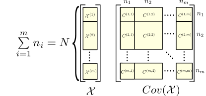
Figure 1: The block structure of the random vector $\mathcal{X}$ and the corresponding covariance block structure.

For a vector, $w\in\mathbb{R}^{N}$, define

$$\mathcal{Z}_{i}:=\sum_{j=1}^{n_{i}}\mathcal{X}^{(i)}\left(j\right)w^{(i)}\left(j\right)=\mathcal{X}^{(i)T}\cdot w^{(i)},$$

$\mathcal{Z}_{i}$ is a random variable computed as linear combination of components of $\mathcal{X}^{(i)}$.

Let $\rho\left(x,y\right)$ denote the correlation coefficient between two random variables,

$$\rho\left(x,y\right)=\frac{Cov\left(x,y\right)}{\sqrt{Cov\left(x,x\right)Cov\left(y,y\right)}}$$

The correlation coefficient between $\mathcal{Z}_{i}$ and $\mathcal{Z}_{j}$ can be expressed as:

$$\rho\left(\mathcal{Z}_{i},\mathcal{Z}_{j}\right)=\frac{w^{(i)T}C^{(i,j)}w^{(j)}}{\sqrt{w^{(i)T}C^{(i,i)}w^{(i)}}\sqrt{w^{(j)T}C^{(j,j)}w^{(j)}}}$$

We are now ready to state the problem. In this paper, we deal with the problem of finding an optimal set of vectors $w^{(i)}$ which maximize

$$\sum_{i=1}^{m}\sum_{j=i+1}^{m}\rho\left(\mathcal{Z}_{i},\mathcal{Z}_{j}\right)$$ (SUMCOR)

This is a generalization of Canonical Correlation Analysis where $m=2$. We refer to this problem as Multi-set Canonical Correlation Analysis (MCCA). We refer to each $\mathcal{X}^{(i)}$ as a particular view of some underlying object with the assumption is that random vectors $\mathcal{X}^{(i)}$ share some mutual information (i.e. are not independent). The original sum of correlations optimization problem is:

$$\underset{w\in\mathbb{R}^{N}}{\text{max}} \sum_{i=1}^{m}\sum_{j=i+1}^{m}\frac{w^{(i)T}C^{(i,j)}w^{(j)}}{\sqrt{w^{(i)T}C^{(i,i)}w^{(i)}}\sqrt{w^{(j)T}C^{(j,j)}w^{(j)}}}.$$

The solution to the optimization problem, the set of components, $\left(w^{(1)},\ldots,w^{(m)}\right),$ are referred to as the set of canonical vectors. Observe that the solution is invariant to scaling (only the direction matters): if $\left(w^{(1)},\ldots,w^{(m)}\right)$ is a solution, then $\left(\alpha_{1}\cdot w^{(1)},\ldots,\alpha_{m}\cdot w^{(m)}\right)$ is also a solution for $\alpha_{i}>0$. This means that we have the freedom to impose the constraints $w^{(i)T}C^{(i,i)}w^{(i)}=1$, which only affect the norm of the solutions. We now arrive to an equivalent constrained problem:

$$\underset{w\in\mathbb{R}^{N}}{\text{maximize}} \sum_{i=1}^{m}\sum_{j=i+1}^{m}w^{(i)T}C^{(i,j)}w^{(j)}$$ (1)

subject to $$w^{(i)T}C^{(i,i)}w^{(i)}=1,\quad\forall i=1,\ldots,m.$$

We proceed by multiplying the objective by $2$ and adding a constant $m$, which does not affect the optimal solution. Using the equalities: $w^{(i)T}C^{(i,j)}w^{(j)}=w^{(j)T}C^{(j,i)}w^{(i)}$ and $w^{(i)T}C^{(i,i)}w^{(i)}=1$ we arrive at:

$$\underset{w\in\mathbb{R}^{N}}{\text{maximize}} \sum_{i=1}^{m}\sum_{j=1}^{m}w^{(i)T}C^{(i,j)}w^{(j)}$$ (2)

subject to $$w^{(i)T}C^{(i,i)}w^{(i)}=1,\quad\forall i=1,\ldots,m.$$

This allows us to consider the summation as the quadratic form $w^{T}Cw$.

Let $C^{(i,i)}$ is strictly positive definite, the Cholesky decomposition $C^{(i,i)}=D_{i}^{T}D_{i}$ exists. Using the substitution $\widetilde{w}_{i}:=D_{i}w_{i}$ and defining $A\in\mathbb{R}^{N}$ such that

$$A^{(i,j)}:={D_{i}}^{-T}C^{(i,j)}{D_{j}}^{-1}$$

Here the block structure $b$ is used. As a consequence of the substitution, we have that $A^{(i,i)}=I_{b\left(i\right)}$, where $I$ denotes the $b\left(i\right)$-by-$b\left(i\right)$ identity matrix. Using block vector notation, let $x\in\mathbb{R}^{N},x^{(i)}=\widetilde{w}_{i},\forall i=1,\ldots,m$.

The form of the optimization problem we will finally consider is:

$$\underset{x\in\mathbb{R}^{N}}{\text{max}} x^{T}Ax$$ (QCQP)

subject to $$x^{(i)T}x^{(i)}=1,\quad\forall i=1,\ldots,m,.$$

where $b:=\left(n_{1},\ldots,n_{m}\right)$ encodes the block structure, $A\in\mathbb{S}_{N}^{+}$, $A^{(i,i)}=I_{b\left(i\right)}$.

We started with a formulation (SUMCOR) and arrived to (QCQP). The last optimization problem is simpler to manipulate and will be used to prove the complexity result of (SUMCOR), as well as to obtain a relaxed version of the problem along with some useful bounds. We will also state a local-optimization approach to solving (SUMCOR) based on the (QCQP) problem formulation.

3.1 NP-Hardness

First, we give a reduction to show that this optimization problem is NP-hard. We use a reduction from a general binary quadratic optimization (BQO) problem.

Let $A\in\mathbb{R}^{m\times m}$ the binary quadratic optimization (BQO) problem is

$$\underset{x\in\mathbb{R}^{m}}{\text{max}} x^{T}Ax$$ (BQO)

subject to $$x\left(i\right)^{2}=1,\quad\forall i=1,\ldots,m$$

Many difficult combinatorial optimization problems (for example maximum cut problem and maximum clique problem [8]) can be reduced to BQO [9], which is known to be NP-hard.

We will show that each BQO problem instance can be reduced to an instance of the problem (QCQP). That means that even though the problem (QCQP) has special structure (maximizing a positive-definite quadratic form over a product of spheres) it still falls into the class of problems that are hard (under the assumption that $P\neq NP$). The idea is to start with a general instance of BQO and through a set of simple transformations obtain a specific instance of (QCQP), with a block structure $b=\left(1,\ldots,1\right)$. The simple transformations will transform the BQO matrix $A$ into a correlation matrix, where the optimal solutions will be preserved.

Let us start a BQO with a corresponding general matrix $A\in\mathbb{R}^{m\times m}$. Since $x^{T}Ax=x^{T}\frac{\left(A+A^{T}\right)}{2}x$ we can assume that the matrix $A$ is symmetric. The binary constraints imply that for any diagonal matrix $D$ the quantity $x^{T}Dx=\sum_{i}D\left(i,i\right)$ is constant. This means that for $c>0$ large enough, we can replace the objective with an equivalent objective $x^{T}\left(A+c\cdot I\right)x$ which is a positive-definite quadratic form. If we set $c$ to $\lVert A\rVert_{1}+1$, it guarantees strong diagonal dominance, a sufficient condition for positive definiteness. From now on, we assume that the matrix $A$ in the BQO is symmetric and positive-definite. Let $g=\max_{i}{A\left(i,i\right)}$ and let $D\in\mathbb{R}^{m\times m}$ be a diagonal matrix with elements $D\left(i,i\right)=g-A\left(i,i\right)$.

Then the BQO is equivalent to:

$$\underset{x\in\mathbb{R}^{m}}{\text{max}} x^{T}\frac{\left(A+D\right)}{g}x$$ (3)

subject to $$x\left(i\right)^{2}=1,\quad\forall i=1,\ldots,m.$$

The matrix $\frac{\left(A+D\right)}{g}$ is a correlation matrix since it is a symmetric positive-definite matrix with all diagonal entries equal to $1$. The optimization problem corresponds to a problem of maximizing a sum of pairwise correlations between univariate random variables (using block structure notation: $b\left(i\right)=1,\forall i=1,\ldots,m$). This shows that even the simple case of maximizing the sum of correlations, where the optimal axes are known and only directions need to be determined, is a NP-hard problem.

3.2 Local solutions

Given that the problem is NP-hard and assuming $P\neq NP$, it is natural to use local methods to obtain a perhaps suboptimal solution. In this section, we give an algorithm that provably converges to locally optimal solutions of the problem (QCQP), when the involved matrix $A$ is symmetric and positive-definite and generic (see [2]).

The general iterative procedure is given as Algorithm 1.

Algorithm 1 Horst algorithm

Input: matrix $A\in\mathbb{S}_{N}^{+}$, block structure $b=\left(n_{1},\ldots,n_{m}\right)$, initial vector $x_{0}\in\mathbb{R}^{N}$ with $\lVert x^{(i)}\rVert>0$,

  $x\leftarrow x_{0};$

  for $iter=1$ to $maxiter$ do

     $x\leftarrow Ax;$

     for $i=1$ to $m$ do

        $x^{(i)}\leftarrow\frac{x^{(i)}}{\lVert x^{(i)}\rVert}$

     end for

  end for

Output: $x$

The algorithm can be interpreted as a generalization of the power iteration method (also known as the Von Mises iteration), a classical approach to finding the largest solutions to the eigenvalue problem $Ax=\lambda x$. If the number of views $m=1$, then Algorithm 1 exactly corresponds to the power iteration. Although the algorithm’s convergence is guaranteed under the assumptions mentioned above, the convergence rate is not known. In practice we observe linear convergence, which we demonstrate in figures 2(a), 2(b). In figure 2(a) we generated $1000$ random instances of matrices $A$ with block structure $b=\left(2,2,2,2,2\right)$ and for each matrix we generated a starting point $x_{0}$ and ran the algorithm. The figure depicts the solution change rate on a logarithmic scale ($log_{10}\frac{\lVert x_{old}-x\rVert}{\lVert x\rVert}$). We observe linear convergence with a wide range of rates of convergence (slopes of the lines). Figure 2(b) shows the convergence properties for a fixed matrix $A$ with several random initial vectors $x_{0}$. The problem exhibits a global (reached for $65\%$ initial vectors $x_{0}$) and a local solution (reached in $35\%$ cases), where the global solution paths converge faster (average global solution path slope equals $-0.08$, as opposed to $-0.05$ for the local solution paths).

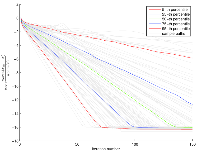
(a)

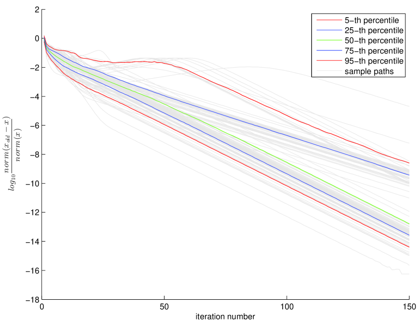
(b)

Figure 2: (a) Convergence plot ($1000$ random matrices $A$, one random $x_{0}$ per problem instance) (b) Convergence plot (single random $A$, $1000$ random initial vectors $x_{0}$)

3.3 Global analysis

The above algorithm is highly scalable and as we shall see in Section 5 often works well in practice. However the algorithm may not converge to a globally optimal solution. We will first present the semidefinite programming relaxation of the problem in 3.3.1. There we will show how the SDP solution can be used to extract solution candidates for the original problem. We will prove a bound that relates the extracted solution quality and the optimal QCQP objective value.

We will then present a set of upper bounds on the optimal QCQP objective value 3.3.2. Such bounds can be used as certificates of optimality (or closeness to optimality) of local solutions (obtained by the local iterative approach for example).

3.3.1 Semidefinite programming relaxation

SDP Relaxation Let $A,B_{1},\ldots,B_{m}\in\mathbb{R}^{N\times N}$ share the block structure $b:=\left(n_{1},\ldots,n_{m}\right),\sum_{i}b\left(i\right)=N$. The blocks $B_{i}^{(k,l)}\in\mathbb{R}^{n_{k}\times n_{l}}$ for $i,k,l=1,\ldots,m$ are defined as:

$$B_{i}^{(k,l)}:=\left\{\begin{array}[]{l l}I_{n_{i}}&:k=i,l=i\\ 0_{k,l}&:else\end{array}\right.$$

where $I_{n_{i}}\in R^{n_{i}\times n_{i}}$ is an identity matrix and $0_{k,l}\in\mathbb{R}^{k,l}$ is a matrix with all entries equal to zero.

Using the fact that $x^{T}Ax=\mathrm{trace}\left(Axx^{T}\right)$ we can rewrite the problem (QCQP) as:

$$\underset{x\in\mathbb{R}^{n}}{\text{max}} \mathrm{trace}\left(Axx^{T}\right)$$ (QCQP2)

subject to $$\mathrm{trace}\left(B_{i}xx^{T}\right)=1,\quad\forall i=1,\ldots,m$$

We can substitute the matrix $xx^{T}$ with a general matrix $X\in\mathbb{S}_{+}^{n}$ constrained it to being rank-one:

$$\underset{X\in\mathbb{S}_{+}^{n}}{\text{maximize}} \mathrm{trace}\left(AX\right)$$

subject to $$\mathrm{trace}\left(B_{i}X\right)=1,\quad\forall i=1,\ldots,m$$

$$\mathrm{rank}\left(X\right)=1.$$

• Matrices $A$ and $B_{1},\ldots,B_{m}$ are symmetric positive-semidefinite matrices.

By omitting the rank-one constraint we obtain a semi-definite program in standard form:

$$\underset{X\in\mathbb{S}_{+}^{n}}{\text{max}} \mathrm{trace}\left(AX\right)$$ (SDP)

subject to $$\mathrm{trace}\left(B_{i}X\right)=1,\quad\forall i=1,\ldots,m.$$

• If the solution of the problem (SDP) is rank-one, i.e. $X$ can be expressed as $X=y\cdot y^{T}$, then $y$ is the optimal solution for (QCQP).

Low rank solutions In the following subsection we will show how to extract solutions to QCQP from solutions of the SDP problem. We will present a bound that relates the global SDP bound, the quality of the extracted solution and the optimal value of QCQP. The bound will tell us how the extracted solution gets close to the optimal QCQP solution when the SDP solution is close to rank 1.

Let $X^{*}$ be a solution to the problem (SDP) and let $x^{*}$ be the solution to the problem (QCQP). Then the following inequality always holds:

$$\mathrm{trace}\left(AX^{*}\right)\geq\mathrm{trace}\left(A\cdot x^{*}\cdot x^{*T}\right).$$

An easy way to extract a good feasible solution to the problem (QCQP) from $X^{*}$ is to project its leading eigenvector to the set of constraints. Let $b=\left(n_{1},\ldots,n_{m}\right),\sum_{i}n_{i}=N$ denote the block structure.

Let $y\in\mathbb{R}^{N},\lVert y^{(i)}\rVert\neq 0$. The projection of vector $y$ to the feasible set of the problem (QCQP) is given by map $\pi\left(\cdot\right):\mathbb{R}^{N}\rightarrow\mathbb{R}^{N}$, defined as:

$$\pi\left(y\right):=\left(\frac{y^{(1)}}{\lVert y^{(1)}\rVert},\ldots,\frac{y^{(m)}}{\lVert y^{(m)}\rVert}\right).$$

The quality of the solution depends on spectral properties of matrix $X$ and matrix $A$.

Assumption 3.1

Let $b=\left(n_{1},\ldots,n_{m}\right)$ denote the block structure and $\sum_{i}n_{i}=N$. Let $X^{*}$ be the solution to the problem (SDP). Let $x_{k}$ denote the $k$-th eigenvector of $X^{*}$. The assumption is the following:

$$\lVert x_{1}^{(i)}\rVert>0,\forall i=1,\ldots,m.$$

Conjecture 3.2

Assumption 3.1 holds in general for optimal solutions to the problem (SDP).

The assumption makes the projection to the feasible set, $\pi(\cdot)$, well defined. In our experiments, this was always true, but we have been unable to find a proof. The result that we will state after the next lemma is based on the projection operator and thus relies on the assumption.

Lemma 3.3

Let $b=\left(n_{1},\ldots,n_{m}\right)$ denote the block structure and $\sum_{i}n_{i}=N$. Let $X^{*}$ be the solution to problem (SDP). Let $x_{k}$ denote the $k$-th eigenvector of $X^{*}$. Let $\alpha_{i}:=\frac{1}{\lVert x_{1}^{(i)}\rVert}$. If $X^{*}$ can be expressed as:

$$X^{*}=\lambda_{1}x_{1}x_{1}^{T}+\lambda_{2}x_{2}x_{2}^{T},$$

where $x_{1}$ and $x_{2}$ have unit length and $\lambda_{1}>1>\lambda_{2}$, then

$$\lambda_{1}\leq\alpha_{i}\alpha_{j}\leq\frac{\lambda_{1}}{1-\lambda_{2}}.$$

• The constraints in problem (SDP) are equivalent to:

  $$\lambda_{1}\lVert x_{1}^{(i)}\rVert^{2}+\lambda_{2}\lVert x_{2}^{(i)}\rVert^{2}=1,\forall i=1,\ldots,m.$$

  Since $\lambda_{2}<1$ and $\lVert x_{2}^{(i)}\rVert^{2}\leq 1$ it follows that $0\leq\lambda_{2}\lVert x_{2}^{(i)}\rVert^{2}<1$. It follows that:

  $$0<\frac{1-\lambda_{2}}{\lambda_{1}}<\lVert x_{2}^{(i)}\rVert^{2}\leq\frac{1}{\lambda_{1}}.$$

  Since $\alpha_{i}=\frac{1}{x_{1}^{(i)}}$ it follows that

  $$\sqrt{\lambda_{1}}\leq\alpha_{i}\leq\sqrt{\frac{\lambda_{1}}{1-\lambda_{2}}},$$

  and finally:

  $$\lambda_{1}\leq\alpha_{i}\alpha_{j}\leq\frac{\lambda_{1}}{1-\lambda_{2}},\forall i,j=1,\ldots,m.$$

   

Proposition 3.4

Let $b=\left(n_{1},\ldots,n_{m}\right)$ denote the block structure and $\sum_{i}n_{i}=N$. Let $X^{*}$ be the solution to the problem (SDP) and $x^{*}$ be the solution to the problem (QCQP). Let $x_{k}$ denote the $k$-th eigenvector of $X^{*}$. Let $\alpha_{i}:=\frac{1}{\lVert x_{1}^{(i)}\rVert}$. Let $\psi:=\mathrm{trace}\left(AX^{*}\right)$, $\phi:=\mathrm{trace}\left(A\cdot x^{*}\cdot x^{*T}\right)$. It is obvious that:

$$\psi\geq\phi\geq\pi\left(x_{1}\right).$$

If $X^{*}$ can be expressed as:

$$X^{*}=\lambda_{1}x_{1}x_{1}^{T}+\lambda_{2}x_{2}x_{2}^{T},$$

where $x_{1}$ and $x_{2}$ have unit length and $\lambda_{1}>1>\lambda_{2}$, then:

$$\psi-\pi\left(x_{1}\right)\leq\left(\frac{1}{1-\lambda_{2}}-1\right)m^{2}+\lambda_{2}\lVert A\rVert_{2}.$$

• $$\psi -\pi\left(x_{1}\right)=\lambda_{1}\sum_{i,j}x_{1}^{(i)T}A^{(i,j)}x_{1}^{(j)T}+$$

  $$\lambda_{2}\sum_{i,j}x_{2}^{(i)T}A^{(i,j)}x_{2}^{(j)T}-\sum_{i,j}\alpha_{i}\alpha_{j}x_{1}^{(i)T}A^{(i,j)}x_{1}^{(j)T}\leq$$

  $$\leq\sum_{i,j}(\lambda_{1}-\alpha_{i}\alpha_{j})x_{1}^{(i)T}A^{(i,j)}x_{1}^{(j)T}+\lambda_{2}\lVert A\rVert_{2}\leq$$

  $$\leq-\sum_{i,j}(\lambda_{1}-\alpha_{i}\alpha_{j})\cdot|x_{1}^{(i)T}A^{(i,j)}x_{1}^{(j)T}|+\lambda_{2}\lVert A\rVert_{2}\leq$$

  $$\leq\left(\frac{\lambda_{1}}{1-\lambda_{2}}-\lambda_{1}\right)\cdot\sum_{i,j}\frac{1}{\alpha_{i}\alpha_{j}}+\lambda_{2}\lVert A\rVert_{2}\leq$$

  $$\leq\left(\frac{\lambda_{1}}{1-\lambda_{2}}-\lambda_{1}\right)\cdot\frac{m^{2}}{\lambda_{1}}+\lambda_{2}\lVert A\rVert_{2}=$$

  $$=\left(\frac{1}{1-\lambda_{2}}-1\right)\cdot m^{2}+\lambda_{2}\lVert A\rVert_{2}$$

   

A similar bound can be derived for the general case, provided that the solution to problem (SDP) is close to rank-one.

Proposition 3.5

Let $b=\left(n_{1},\ldots,n_{m}\right)$ denote the block structure and $\sum_{i}n_{i}=N$. Let $X^{*}$ be the solution to the problem (SDP) and $x^{*}$ be the solution to the problem (QCQP). Let $x_{k}$ denote the $k$-th eigenvector of $X^{*}$. Let $\alpha_{i}:=\frac{1}{\lVert x_{1}^{(i)}\rVert}$. Let $\psi:=\mathrm{trace}\left(AX^{*}\right)$. If $X^{*}$ can be expressed as:

$$X^{*}=\lambda_{1}x_{1}x_{1}^{T}+\lambda_{2}x_{2}x_{2}^{T}+\cdots+\lambda_{n}x_{n}x_{n}^{T},$$

where each $x_{i}$ has unit length and $\lambda_{1}>1>\underset{i=2,\ldots,n}{\sum}\lambda_{i}$, then:

$$\psi -\pi\left(x_{1}\right)$$

$$\leq\left(\frac{1}{1-\underset{i=2,\ldots,n}{\sum}\lambda_{i}}-1\right)m^{2}+\left(\underset{i=2,\ldots,n}{\sum}\lambda_{i}\right)\lVert A\rVert_{2}.$$

3.3.2 Upper bounds on QCQP

This subsection will present several upper bounds on the optimal QCQP objective value. We will state a simple upper bound based on the spectral properties of the QCQP matrix $A$. We will then bound the possible values of the SDP solutions and present two constant relative accuracy bounds.

$L_{2}$ norm bound We will present an upper bound on the objective of (QCQP) based on the largest eigenvalue of the problem matrix $A$.

Proposition 3.6

The objective value of (QCQP) is upper bounded by $m\cdot\lVert A\rVert_{2}$.

• The problem (QCQP) remains the same if we add a redundant constraint $x^{T}x=m$ obtained by summing the constraints $\sum_{i=1}^{m}\left(x^{(i)T}x^{(i)}-1\right)=0$. We then relax the problem by dropping the original constraints to get:

  $$\underset{x\in\mathbb{R}^{N}}{\text{max}} x^{T}Ax$$ (4)

  subject to $$x^{T}x=m.$$

  Since $\lVert A\rVert_{2}=\text{max}_{\lVert x\rVert_{2}=1}x^{T}Ax$ it follows that the optimal objective value of (4) equals $m\cdot\lVert A\rVert_{2}$.       

Bound on possible SDP objective values

Lemma 3.7

Let $X^{*}$ be the solution to the problem (SDP) and let $\psi:=\mathrm{trace}\left(AX^{*}\right)$. Then

$$m\leq\psi\leq m^{2}.$$

• Express $X^{*}$ as:

  $$X^{*}=\underset{i=1,\ldots,n}{\sum}\lambda_{i}x_{i}x_{i}^{T},$$

  where each $x_{i}$ has unit length and $\lambda_{1}\geq\ldots\geq\lambda_{N}\geq 0$. The lower bound follows from the fact that $\psi$ upper bounds the optimal objective value of problem (QCQP) which is lower bounded by $m$. The lower bound corresponds to the case of zero sum of correlations.

  To prove the upper bound first observe that the constraints in (SDP) imply that $\underset{i=1,\ldots,n}{\sum}\lambda_{i}=m$. Let $y\in\mathbb{R}^{N}$ and let $\lVert y\rVert_{2}=1$. Let $z:=\left(\lVert y^{(1)}\rVert,\ldots,\lVert y^{(m)}\rVert\right)^{T}.$ Observe that $\lVert z\rVert_{2}=1$ and that $\lVert zz^{T}\rVert_{2}=1$. Define $e\in\mathbb{R}^{m},e\left(i\right)=1,\forall i=1,\ldots,m$. We will now bound $\lVert A\rVert_{2}$:

  $$y^{T}Ay =\sum_{i,j=1,\ldots,m}y^{(i)T}A^{(i,j)}y^{(j)}$$

  $$=\sum_{i,j=1,\ldots,m}\lVert y^{(i)}\rVert\lVert y^{(j)}\rVert\frac{y^{(i)T}}{\lVert y^{(i)}\rVert}A^{(i,j)}\frac{y^{(j)}}{\lVert y^{(j)}\rVert}\leq$$

  $$\leq\sum_{i,j=1,\ldots,m}\lVert y^{(i)}\rVert\lVert y^{(j)}\rVert$$

  $$=e^{T}(zz^{T})e\leq\lVert e\rVert\cdot\lVert zz^{T}\rVert_{2}\cdot\lVert e\rVert=m.$$

  We used the fact that $\frac{y^{(i)T}}{\lVert y^{(i)}\rVert}A^{(i,j)}\frac{y^{(j)}}{\lVert y^{(j)}\rVert}$ is a correlation coefficient and thus bounded by $1$. The upper bound follows:

  $$\mathrm{trace}\left(AX^{*}\right)=\mathrm{trace}\left(A\underset{i=1,\ldots,n}{\sum}\lambda_{i}x^{(i)}x^{(i)T}\right)=$$

  $$=\underset{i=1,\ldots,n}{\sum}\lambda_{i}x^{(i)T}Ax^{(i)}\leq\underset{i=1,\ldots,n}{\sum}\lambda_{i}\cdot m=m^{2}.$$

   

Constant relative accuracy guarantee We now state a lower bound on the ratio between the objective values of the original and the relaxed problem that is independent on the problem dimension. The bound is based on the following result from [22], stated with minor differences in notation. Let $\mathrm{Square}(\cdot)$ denote componentwise squaring: if $y=\mathrm{Square}(x)$ then $y(i)=x(i)^{2}$ and let $\mathrm{diag}(X)$ denote the vector corresponding to the diagonal of the matrix $X$.

Theorem 3.8

Let $A\in\mathbb{R}^{N\times N}$ be symmetric and let $\mathcal{F}$ be a set with the following properties:

• $\mathcal{F}$ is closed, convex and bounded.

• There exists a strictly positive $v\in\mathcal{F}$.

• $\mathcal{F}=\left\{v\in K:Bv=c\right\},$ where $K$ is a convex closed pointed cone in $\mathbb{R}^{N}$ with non-empty interior, $B\in\mathbb{R}^{k\times N}$, $c\neq 0_{k}$ and $\left\{v\in\mathrm{int}K:Bv=c\right\}\neq\emptyset$.

Let

$$\phi^{*} :=\mathrm{max}\left\{x^{T}Ax:\mathrm{square}\left(x\right)\in\mathcal{F}\right\},$$

$$\phi_{*} :=\mathrm{min}\left\{x^{T}Ax:\mathrm{square}\left(x\right)\in\mathcal{F}\right\},$$

$$\psi^{*} :=\mathrm{max}\left\{\mathrm{trace}\left(AX\right):\mathrm{diag}\left(X\right)\in\mathcal{F},X\in\mathbb{S}_{N}^{+}\right\},$$

$$\psi_{*} :=\mathrm{min}\left\{\mathrm{trace}\left(AX\right):\mathrm{diag}\left(X\right)\in\mathcal{F},X\in\mathbb{S}_{N}^{+}\right\},$$

$$\psi\left(\alpha\right) :=\alpha\psi^{*}+\left(1-\alpha\right)\psi_{*}.$$

Then

$$\psi_{*}\leq\phi_{*}\leq\psi\left(1-\frac{2}{\pi}\right)\leq\psi\left(\frac{2}{\pi}\right)\leq\phi^{*}\leq\psi^{*}.$$

Theorem 3.9

Let $x^{*}$ be the solution to the problem (QCQP2) and $X^{*}$ be the solution to the problem (SDP). Let $b=\left(n_{1},\ldots,n_{m}\right)$ denote the block structure where $\sum_{i}n_{i}=N$. Let $\phi^{*}:=\mathrm{trace}\left(A\cdot x^{*}\cdot x^{*T}\right)$, $\psi^{*}:=\mathrm{trace}\left(AX^{*}\right)$.

Then

$$\frac{2}{\pi}\psi^{*}\leq\phi^{*}\leq\psi^{*}.$$

• We first note that $\psi_{*}\geq 0$, since $A\in\mathbb{S}_{+}^{n}$. This follows from the fact that $\mathrm{trace}\left(AX\right)\geq 0$ for any $X\in\mathbb{S}_{+}^{n}$ (and thus for the minimizer $X_{*}$). The positiveness of the trace can be deduced from: $\mathrm{trace}\left(AX\right)=\mathrm{trace}\left(C_{A}C_{A}^{T}C_{X}C_{X}^{T}\right)=\mathrm{trace}\left(C_{X}^{T}C_{A}C_{A}^{T}C_{X}\right)=\lVert C_{A}^{T}C_{X}\rVert_{F}^{2}\geq 0$, where $C_{A}$ and $C_{X}$ are Cholesky factors of matrices $A$ and $X$ respectively.

  We now show that the problems (QCQP2) and (SDP) can be reformulated so that the theorem 3.8 applies.

  First we note that the feasible sets in (QCQP2) and (SDP) are defined in terms of equalities. Without loss of generality we can replace them with inequality constraints: $x^{(i)T}x^{(i)}\leq 1$ in (QCQP2) and $\mathrm{trace}\left(B_{i}X\right)\leq 1$ in (SDP). The feasible sets defined by the inequalities are convex and bounded. Since the objective functions in both problems are convex, it follows that the optima lie on the border.

  Next, we add redundant constraints to the two problems respectively: $\mathrm{Square}\left(x^{(i)}\right)\geq 0,\forall i=1,\ldots,m$ and $X\left(j,j\right)\geq 0,\forall j=1,\ldots,N$.

Define $\mathcal{F}=\left\{x\in\mathbb{R}^{N}|x^{(i)}\in\Delta^{n_{i}-1}\right\}$, where

$$\Delta^{k}=\left\{x\in\mathbb{R}^{k+1}|x\left(i\right)\geq 0,\forall i~{}\mathrm{and}~{}\sum_{i}x\left(i\right)=1\right\}.$$

$\mathcal{F}$ is a product of standard simplices: $\mathcal{F}=\prod_{i=1}^{m}\Delta^{n_{i}-1}$. It follows that the set is closed, bounded and convex. $\mathcal{F}$ can be embedded in $\mathbb{R}^{N+1}$ in order to obtain a conic formulation.

$$K=\{t\cdot\left[1~{}x^{T}\right]^{T} |t\geq 0,x\in\mathcal{F}\}$$

$$B=\left[1~{}0_{N}^{T}\right]^{T},\quad c=1, \quad\widetilde{\mathcal{F}}=K\cap\left\{x|Bx=c\right\}.$$

Define $v=\left[v_{1}^{T}\ldots v_{m}^{T}\right]^{T},$ where $v_{i}\left(j\right)=\frac{1}{n_{i}}$. The vector $\left[1~{}v^{T}\right]^{T}$ is strictly positive and lies in $\mathrm{int}\left(K\right)\cap\left\{x\in\mathbb{R}^{N+1}|Bx=c\right\}$. Let $\widetilde{A}\in\mathbb{R}^{N+1}$ be defined as $\widetilde{A}\left(1,i\right)=0$, $\widetilde{A}\left(i,1\right)=0,\forall i$ and $\widetilde{A}\left(i,j\right)=A\left(i-1,j-1\right),\forall i,j>1$.

The optimization problem (QCQP2) is equivalent(with the same optimal objective value) to:

$$\underset{x\in\mathbb{R}^{N+1}}{\text{max}} \mathrm{trace}\left(\widetilde{A}xx^{T}\right)$$

subject to $$\mathrm{Square}\left(x\right)\in\widetilde{F}$$

The optimization problem (SDP) is likewise equivalent to the problem:

$$\underset{X\in\mathbb{S}_{+}^{N+1}}{\text{max}} \mathrm{trace}\left(\widetilde{A}X\right)$$

subject to $$\mathrm{diag}\left(X\right)\in\widetilde{F}$$

Using the definition of $\psi\left(\alpha\right)$ and the fact that $\psi_{*}\geq 0$ it follows that $\psi\left(\alpha\right)\geq\alpha\psi^{*},\forall\alpha\geq 0$. Substituting $\alpha=\frac{2}{\pi}$ we get the desired result:

$$\frac{2}{\pi}\psi^{*}\leq\phi^{*}\leq\psi^{*}.$$

 

Observe that the bound above relates the optimization problems (QCQP) and (SDP) and not (1) with its SDP relaxation. Let $\widetilde{\phi}$ denote the optimum value of the objective function in (1) and let $\widetilde{\psi}$ denote the optimum value of the objective function of the corresponding SDP relaxation. It is easy to see that $2\cdot\widetilde{\phi}+m=\phi$ and $2\cdot\widetilde{\psi}+m=\psi$, which is a consequence of transformations of the original problems to their equivalent symmetric positive-definite problems. The $\frac{2}{\pi}$ constant relative accuracy bound becomes a bit weaker in terms of the original problem and its relaxation. This fact is stated in the following corollary.

Corollary 3.10

$$\widetilde{\phi}\geq\frac{2}{\pi}\widetilde{\psi}-\frac{(1-\frac{2}{\pi})m}{2}.$$

Improved bound on the relative accuracy We can exploit additional structure of the problem to obtain a slightly better bound. We use the same conventions as [22].

Define

$$\omega\left(\beta\right):=\beta\arcsin\left(\beta\right)+\sqrt{1-\beta^{2}}.$$

The function $\omega\left(\beta\right)$ is increasing and convex with $\omega\left(0\right)=1$ and $\omega\left(1\right)=\frac{\pi}{2}$.

By theorem 3.1, item 1 in [22] we obtain the result:

$$\max\left\{\frac{2}{\pi}\omega\left(\frac{m}{\psi^{*}}\right),\frac{m}{\psi^{*}}\right\}\psi^{*}\leq\phi^{*}\leq\psi^{*}.$$

This results in a minor improvement of the default bound. For example when $m=3$ and the fact that $\frac{m}{\psi^{*}}\geq\frac{1}{3}$ we obtain the following:

$$\frac{2}{\pi}\psi^{*}\leq\frac{105}{100}\cdot\frac{2}{\pi}\psi^{*}\leq\phi^{*}\leq\psi^{*}$$

4 Sum of correlations extensions

In this section we discuss two extensions of MCCA. By using kernel methods we show how to find nonlinear dependencies in the data. We then present an extension of the method to finding more then one set of correlation vectors.

4.1 Dual representation and kernels

We return to the formulation (1):

$$\underset{w\in\mathbb{R}^{N}}{\text{max}} \sum_{i=1}^{m}\sum_{j=i+1}^{m}w^{(i)T}C^{(i,j)}w^{(j)}$$

subject to $$w^{(i)T}C^{(i,i)}w^{(i)}=1,\quad\forall i=1,\ldots,m,$$

where $b=\left(n_{1},\ldots,n_{m}\right)$ denotes the block structure and $\sum_{i}n_{i}=N$. In the previous sections we focused on manipulating covariance matrices only and omitted details on their estimation based on finite samples. In this section we will use a formulation that explicitly presents the empirical estimates of covariances, which will enable us to apply kernel methods. Let $\mathcal{X}$ be a random vector distributed over $\mathbb{R}^{N}$ with $E\left(\mathcal{X}\right)=0$. Let $X\in\mathbb{R}^{N\times s}$ represent a sample of $s$ observations of $\mathcal{X}$, where each observation corresponds to a column vector. Empirical covariance of $\mathcal{X}$ based on the sample matrix $X$ is expressed as:

$$\overline{Cov\left(\mathcal{X}\right)}=\frac{1}{s-1}XX^{T}.$$

In case the number of number of observations, $s$, is smaller than the total number of dimensions $N$, the covariance matrix $\overline{Cov\left(\mathcal{X}\right)}$ is singular. This is problematic both from a numerical point of view and it leads to overfitting problems. These issues are addressed by using regularization techniques, typically a shrinkage estimator $\overline{Cov\left(\mathcal{X}\right)_{\kappa}}$ is defined as:

$$\overline{Cov\left(\mathcal{X}\right)_{\kappa}}=\left(1-\kappa\right)\frac{1}{s-1}XX^{T}+\kappa I_{N},$$

where $\kappa\in\left[0,1\right]$.

Using the block structure $b$, (2) becomes:

$$\underset{w\in\mathbb{R}^{N}}{\text{max}} \frac{1}{s-1}\sum_{i=1}^{m}\sum_{j=i+1}^{m}w^{(i)T}X^{(i)}X^{(j)T}w^{(j)}$$ (5)

subject to $$w^{(i)T}\left(\frac{1-\kappa}{s-1}X^{(i)}X^{(i)T}+\kappa I_{N}\right)w^{(i)}=1,$$

$$\quad\forall i=1,\ldots,m.$$

We will now express each component $w^{(i)}$ in terms the columns of $X^{(i)}$. Let $w$ have block structure $b_{w}=\left(n_{1},\ldots,n_{m}\right)$ where $\sum_{i}n_{i}=N$, and let $y\in\mathbb{R}^{m\cdot s}$ have block structure $b_{y}\left(i\right)=s,\forall i=1,\ldots,m$.

$$w^{(i)}=\sum_{j=1}^{s}y^{(i)}\left(j\right)X^{(i)}\left(:,j\right)=X^{(i)}y^{(i)},$$ (6)

We refer to $y$ as dual variables.

Lemma 4.1

Solutions to the problem (5) can be expressed as (6).

• We will prove this by contradiction. Let $u$ be the optimal solution to (5). Assume that $u^{(1)}$ doesn’t lie in the column space of $X^{(1)}$,

  $$u^{(1)}=z_{\bot}+X^{(1)}y^{(1)},$$

  where

  $$z_{\bot}\neq 0_{n_{1}}\quad\text{and}\quad X^{(1)T}z_{\bot}=0_{s}.$$

  Then $\bar{u}$ defined as $\bar{u}^{(i)}=u^{(i)},\forall i>1$ and $\bar{u}^{(1)}=\frac{1}{\gamma}X^{(1)}y^{(1)},$ where

  $$\gamma=\sqrt{y^{(1)T}X^{(1)T}\left(\frac{1-\kappa}{s-1}X^{(1)}X^{(1)T}+\kappa I_{N}\right)X^{(1)}y^{(1)}}$$

  strictly increases the objective function, which contradicts $u$ being optimal. Clearly $\bar{u}$ is a feasible solution. Positive definiteness of $\frac{1-\kappa}{s-1}X^{(1)}X^{(1)T}+\kappa I_{N}$ coupled with the fact that $z_{\bot}^{T}z_{\bot}>0$ implies that $0<\gamma<1$. Assume without loss of generality that $\sum_{j=2}^{m}\left(X^{(1)}y^{(1)}\right)^{T}X^{(1)}X^{(j)T}u^{(j)}>0$ (The negative sum would lead to another contradiction by taking $\bar{u}^{(1)}=-u^{(1)}$. If the sum was zero, then any properly scaled (with proper sign) combination of the training data $X^{(1)}$ could be used in place of $u^{(1)}$). The following inequality completes the proof:

  $$\frac{1}{s-1} \sum_{j=2}^{m}u^{(1)T}X^{(1)}X^{(j)T}u^{(j)}=$$

  $$=\frac{1}{s-1} \sum_{j=2}^{m}\left(z_{\bot}+X^{(1)}y^{(1)}\right)^{T}X^{(1)}X^{(j)T}u^{(j)}=$$

  $$=\frac{1}{s-1} \sum_{j=2}^{m}\left(X^{(1)}y^{(1)}T\right)X^{(1)}X^{(j)T}u^{(j)}<$$

  $$<\frac{1}{s-1} \sum_{j=2}^{m}\frac{1}{\gamma}\left(X^{(1)}y^{(1)}\right)^{T}X^{(1)}X^{(j)T}u^{(j)}.$$

   

Let $K_{i}=X^{(i)T}X^{(i)}\in\mathbb{R}^{s\times s}$ denote the Gram matrix. We now state regularized covariance formulation (5) in terms of the dual variables:

$$\underset{y\in\mathbb{R}^{m\cdot s}}{\text{max}} \frac{1}{s-1}\sum_{i=1}^{m}\sum_{j=i+1}^{m}y^{(i)T}K_{i}K_{j}^{T}y^{(j)}$$ (7)

subject to $$y^{(i)T}\left(\frac{1-\kappa}{s-1}K_{i}K_{i}^{T}+\kappa K_{i}\right)y^{(i)}=1,$$

$$\quad\forall i=1,\ldots,m.$$

The problem is reformulated in terms of Gram matrices based on the standard inner product. This formulation lends itself to using kernel methods (see [27]) which enable discovering nonlinear patterns in the data.

Typically the matrices $K_{i}$ are ill conditioned (even singular when the data is centered) and it is advantageous to constrain the magnitude of dual coefficients as well as the variance in the original problem. We address this by introducing a first order approximation to the dual regularized variance. Let

$$\widetilde{K_{i}}:=\left(\sqrt{\frac{1-\kappa}{s-1}}K_{i}+\frac{\kappa}{2}\sqrt{\frac{s-1}{1-\kappa}}I_{s}\right).$$

Then:

$$\overline{Cov\left(\mathcal{X}^{(i)}\right)_{\kappa}}=\frac{1-\kappa}{s-1}K_{i}K_{i}^{T}+\kappa K_{i}\approx\widetilde{K_{i}}\widetilde{K_{i}}^{T}.$$

The approximation that has two advantages: it is invertible and factorized, which we exploit in obtaining a convergent local method. The final optimization is then expressed as:

$$\underset{y\in\mathbb{R}^{m\cdot s}}{\text{max}} \frac{1}{s-1}\sum_{i=1}^{m}\sum_{j=i+1}^{m}y^{(i)T}K_{i}K_{j}^{T}y^{(j)}$$ (8)

subject to $$y^{(i)T}\widetilde{K_{i}}\widetilde{K_{i}}^{T}y^{(i)}=1,\quad\forall i=1,\ldots,m.$$

The problem can be interpreted as maximizing covariance while constraining variance and magnitude of dual coefficients.

4.2 Computing several sets of canonical vectors

Usually a one-dimensional representation does not sufficiently capture all the information in the data and higher dimensional subspaces are needed. After computing the first set of primal canonical vectors we proceed to computing the next set. The next set should be almost as highly correlated as the first one, but essentially “different” from the first one. We will achieve this by imposing additional constraints for every view, namely that all projection vectors in view $i$ are uncorrelated with respect to $\widetilde{K}_{i}^{2}$ (similar as in two view regularized kernel CCA, see [17]).

Let $Y=\left[y_{1},\ldots,y_{k}\right]\in\mathbb{R}^{m\cdots\times k}$ represent $k$ sets of canonical vectors, where

$$Y^{(\ell)T}\widetilde{K_{\ell}^{2}}Y^{(\ell)}=I_{k}\forall\ell=1,\ldots,m.$$

The equation above states that each canonical vector has unit regularized variance and that different canonical vectors corresponding to the same view are uncorrelated (orthogonal with respect to $\widetilde{K_{i}^{2}}$).

We will now extend the set of constraints in the optimization (8) to enforce the orthogonality.

$$\underset{y\in\mathbb{R}^{m\cdot s}}{\text{max}} \frac{1}{s-1}\sum_{i=1}^{m}\sum_{j=i+1}^{m}y^{(i)T}K_{i}K_{j}^{T}y^{(j)}$$ (9)

subject to $$y^{(i)T}\widetilde{K_{i}}\widetilde{K_{i}}^{T}y^{(i)}=1,\quad\forall i=1,\ldots,m$$

$$Y^{(i)T}\widetilde{K_{i}}\widetilde{K_{i}}^{T}y^{(i)}=0_{k},\quad\forall i=1,\ldots,m.$$

In order to use the Horst algorithm, we first use substitutions:

$$Z^{(i)}=\widetilde{K_{i}}Y^{(i)},\quad z^{(i)}=\widetilde{K_{i}}y^{(i)}.$$

We then define operators

$$P_{i}=I_{s}-\widetilde{K}_{i}Y^{(i)}Y^{(i)T}\widetilde{K}_{i}=I_{s}-Z^{(i)}Z^{(i)T},$$

which map to the space orthogonal to the columns of $\widetilde{K}_{i}Y^{(i)}$. Each $P_{i}$ is a projection operator: $P_{i}^{2}=P_{i},$ which follows directly from the identities above. We restate the optimization problem in the new variables:

$$\underset{z\in\mathbb{R}^{m\cdot s}}{\text{max}} \frac{1}{s-1}\sum_{i=1}^{m}\sum_{j=i+1}^{m}z^{(i)T}\widetilde{K_{i}}^{-T}K_{i}K_{j}^{T}\widetilde{K_{j}}^{-1}z^{(j)}$$ (10)

subject to $$z^{(i)T}z^{(i)}=1,\quad\forall i=1,\ldots,m$$

$$Z^{(i)T}z^{(i)}=0_{k},\quad\forall i=1,\ldots,m.$$

By using the projection operators, the optimization problem is equivalent to:

$$\underset{z\in\mathbb{R}^{m\cdot s}}{\text{max}} \frac{1}{s-1}\sum_{i=1}^{m}\sum_{j=i+1}^{m}z^{(i)T}P_{i}^{T}\widetilde{K_{i}}^{-T}K_{i}K_{j}^{T}\widetilde{K_{j}}^{-1}P_{j}z^{(j)}$$

s.t. $$z^{(i)T}z^{(i)}=1,\quad\forall i=1,\ldots,m.$$

By multiplying the objective by $2$ (due to symmetries of $P_{i},K_{i}$ and $\widetilde{K_{i}}$) and shifting the objective function by $\frac{m}{1-\kappa}$, the problem is equivalent to:

$$\underset{z\in\mathbb{R}^{m\cdot s}}{\text{max}} \frac{1}{s-1}\sum_{i=1}^{m}\sum_{\begin{subarray}{c}j=1\\ j\neq i\end{subarray}}^{m}z^{(i)T}P_{i}^{T}\widetilde{K_{i}}^{-T}K_{i}K_{j}^{T}\widetilde{K_{j}}^{-1}P_{j}z^{(j)}$$ (11)

$$+\frac{1}{1-\kappa}\sum_{i=1}^{m}z^{(i)T}z^{(i)}$$

s.t. $$z^{(i)T}z^{(i)}=1,\quad\forall i=1,\ldots,m.$$

This last optimization can be reformulated as:

$$\underset{z\in\mathbb{R}^{m\cdot s}}{\text{max}} z^{T}Az$$ (12)

subject to $$z^{(i)T}z^{(i)}=1,\quad\forall i=1,\ldots,m,$$

where $A\in\mathbb{R}^{m\cdot s}$ with block structure $b\left(i\right)=s,\forall i=1,\ldots,m$, defined by:

$$A^{(i,j)}=\left\{\begin{array}[]{lll}\frac{1}{s-1}P_{i}^{T}\widetilde{K_{i}}^{-T}K_{i}K_{j}^{T}\widetilde{K_{j}}^{-1}P_{j}&{\rm for}~{}i\neq j\\ \frac{1}{1-\kappa}I_{s}&{\rm for}~{}i=j\end{array}\right\}$$

Lemma 4.2

The block matrix $A$ defined above is positive semidefinite (i.e. $A\in\mathbb{S}_{+}^{m\cdot s}$).

• $A$ is symmetric, which follows from $P_{i}=P_{i}^{T}$ and $K_{i}=K_{i}^{T}$. Let $z\in\mathbb{R}^{m\cdot s}$. We will show that $z^{T}Az>0$. Let $W=\frac{1}{1-\kappa}\sum_{i=1}^{m}z^{(i)T}P_{i}^{T}\widetilde{K_{i}}^{-T}\left(\kappa K_{i}+\frac{\kappa^{2}\left(s-1\right)}{4\left(1-\kappa\right)}I_{s}\right)\widetilde{K_{i}}^{-1}P_{i}z^{(i)}$. Note that $W\geq 0$ (each summand is positive-semidefinite) and $W>0$ if $\exists i:P_{i}z^{(i)}=z^{(i)}$.

  $$z^{T}Az =\frac{1}{s-1}\sum_{i=1}^{m}\sum_{\begin{subarray}{c}j=1\\ j\neq i\end{subarray}}^{m}z^{(i)T}P_{i}^{T}\widetilde{K_{i}}^{-T}K_{i}K_{j}^{T}\widetilde{K_{j}}^{-1}P_{j}z^{(j)}$$

  $$+\frac{1}{1-\kappa}\sum_{i=1}^{m}z^{(i)T}z^{(i)}\geq$$

  $$\geq\frac{1}{s-1}\sum_{i=1}^{m}\sum_{\begin{subarray}{c}j=1\\ j\neq i\end{subarray}}^{m}z^{(i)T}P_{i}^{T}\widetilde{K_{i}}^{-T}K_{i}K_{j}^{T}\widetilde{K_{j}}^{-1}P_{j}z^{(j)}$$

  $$+\frac{1}{1-\kappa}\sum_{i=1}^{m}z^{(i)T}P_{i}^{T}P_{i}z^{(i)}=$$

  $$=\frac{1}{s-1}\sum_{i=1}^{m}\sum_{\begin{subarray}{c}j=1\\ j\neq i\end{subarray}}^{m}z^{(i)T}P_{i}^{T}\widetilde{K_{i}}^{-T}K_{i}K_{j}^{T}\widetilde{K_{j}}^{-1}P_{j}z^{(j)}$$

  $$+\frac{1}{1-\kappa}\sum_{i=1}^{m}z^{(i)T}P_{i}^{T}\widetilde{K_{i}}^{-T}\widetilde{K_{i}}^{T}\widetilde{K_{i}}\widetilde{K_{i}}^{-1}P_{i}z^{(i)}=$$

  $$=\frac{1}{s-1}\sum_{i=1}^{m}\sum_{\begin{subarray}{c}j=1\\ j\neq i\end{subarray}}^{m}z^{(i)T}P_{i}^{T}\widetilde{K_{i}}^{-T}K_{i}K_{j}^{T}\widetilde{K_{j}}^{-1}P_{j}z^{(j)}$$

  $$+\frac{1}{s-1}\sum_{i=1}^{m}z^{(i)T}P_{i}^{T}\widetilde{K_{i}}^{-T}K_{i}K_{i}^{T}\widetilde{K_{i}}^{-1}P_{i}z^{(i)}+W=$$

  $$=z^{T}BB^{T}z+W\geq 0,$$

  where $B\in\mathbb{R}^{m\cdot s\times s}$, defined by $B^{(i)}=\frac{1}{\sqrt{s-1}}(K_{i}\widetilde{K_{i}}^{-1}P_{i})^{T}$, with corresponding row block structure $b\left(i\right)=s,\forall i=1,\ldots,m$. If $P_{i}z^{(i)}\neq z^{(i)}$ for some $i$, then the first inequality is strict ($\lVert P_{i}z^{(i)}\rVert<\lVert z^{(i)}\rVert$). Conversely, if $P_{i}z^{(i)}=z^{(i)}$ for all $i$, then $W>0$, hence the last inequality is strict.      

Since matrix $A$ has all the required properties for convergence, we can apply the Algorithm 1. Solutions to the problem (9) are obtained by back-substitution $y^{(i)}=\widetilde{K_{i}}^{-1}z^{(i)}$.

4.3 Implementation

The algorithm involves matrix vector multiplications and inverted matrix vector multiplications. If kernel matrices are products of sparse matrices: $K_{i}=X^{(i)T}X^{(i)}$ with $X^{(i)}$ having $sn$ elements where $s<<n$, then kernel matrix vector multiplications cost $2ns$ instead of $n^{2}$. We omit computing the full inverses and rather solve the system $K_{i}x=y$ for x, every time $K_{i}^{-1}y$ is needed. Since regularized kernels are symmetric and multiplying them with vectors is fast (roughly four times slower as multiplying with original sparse matrices $X^{(i)}$), an iterative method like conjugate gradient (CG) is suitable. Higher regularization parameters increase the condition number of each $\tilde{K}_{i}$ which speeds up CG convergence.

If we fix the number of iterations, $maxiter$, and number of CG steps, $C$, the computational cost of computing a $k$-dimensional representation is upper bounded by: $O\big{(}C\cdot maxiter\cdot k^{2}\cdot m\cdot n\cdot s\big{)},$ where $m$ is the number of views, $n$ the number of observations and $s$ average number of nonzero features of each observation. Since the majority of computations is focused on sparse matrix-vector multiplications, the algorithm can easily be implemented in parallel (sparse matrices are fixed and can be split into multiple blocks).

So far we have assumed that the data is centered. Centering can efficiently be implemented on the fly with no changes in asymptotic computational complexity, but we will omit the technical details due to space constraints.

5 Experiments

We evaluated the SDP approach on two scenarios: performance analysis on synthetic data and performance on finding a common representation of a cross-lingual collection of documents.

5.1 Synthetic data

We generated several MCCA problem instances by varying the number of views and number the of dimensions per view in order to compare the performance of local search methods and the proposed SDP relaxation. The main purpose of the experiments was to see under which conditions and how likely do the global bounds provide useful information.

Let $m$ denote the number of views (sets of variables) and $n_{i}$ denote the dimensionality of $i$-th view and $N:=\sum_{i}n_{i}$. In all cases we used the same number of dimensions per view ($n_{1}=n_{2}=\cdots=n_{m}$). We used three different methods to generate random correlation matrices.

The first method, the random Gram matrices (see [13], [1]) , generates the correlation matrices by sampling $N$ vectors $v_{1},\ldots,v_{n}$ for a $N$-dimensional multivariate Gaussian distribution (centered at the origin, with an identity covariance matrix), normalizing them and computing the correlation matrix $C=\left[c_{i,j}\right]_{N\times N}$ as $c_{i,j}:=v_{i}^{\prime}\cdot v_{j}$. The second method, the random spectrum, involves sampling the eigenvalues $\lambda_{1},\ldots,\lambda_{N}$ uniformly from a simplex ($\sum_{i=1}^{N}\lambda_{i}=N$) and generating a random correlation matrix with the prescribed eigenvalues (see [1]). The final method, random 1-dim structures, involves generating a correlation matrix that has an approximately (due to noise) single-dimensional correlation structure. Here we generated a random $m$ dimensional Gram matrix $B$, and inserted it into a $N\times N$ identity matrix according to the block structure to obtain a matrix $C_{0}$ (Set $C_{0}\left(i,j\right)=\delta\left(i,j\right)$, where $\delta$ is the Kronecker delta. Then for $I,J=1\ldots,m$ override the entries $C_{0}\left(1+\sum_{i=1}^{I-1}n_{i},1+\sum_{i=1}^{J-1}n_{i}\right)=B\left(I,J\right)$, where we used $1$-based indexing). We then generated a random Gram matrix $D\in\mathbb{R}^{N\times N}$ and computed the final correlation matrix as $C=\left(1-\epsilon\right)C_{0}+\epsilon D$. In our experiments we set $\epsilon=0.001$. The purpose of using a random spectrum method is that as the dimensionality increases, random vectors tend to be orthogonal, hence the experiments based on random Gram matrices might be less informative. As we will see later, the local method suffers the most when all $n_{i}=1$, which is an instance of a BQO problem. By using the approximately 1-dimensional correlation matrix sampling we investigated if the problem persists when $n_{i}>1$.

In all cases we perform a final step that involves computing the per-view Cholesky decompositions of variances and change of basis as we showed when we arrived to QCQP reformulation in equation (QCQP).

The experiments are based on varying the number of sets of variables, $m$, and the dimensionality $n_{i}$. For each sampling scenario and each choice of $m$ and $n_{i}$, we generated $100$ experiments, and computed $1000$ solutions based on Algorithm 1, the SDP solution (and respective global bounds), and looked at the frequencies of the following events:

• a duality gap candidate detected (Tables 1, 2, 3 (a)),

• local convergence detected (Tables 1, 2, 3 (b))

• when a local solution is worse than the SDP-based lower bound (Tables 1, 2, 3 (c)).

The possibility of duality gap is detected when the best local solution is lower than $1\%$ of the SDP bound. In this case the event indicates only the possibility of duality gap – it might be the case that further local algorithm restarts would close the gap. The local convergence event is detected when the objective value of two local solutions differs relatively by at least $10\%$ and absolutely at least by $0.1$ (both criterions have to be satisfied simultaneously). Finally, the event of local solution being bellow the SDP lower bound means that it is bellow $\frac{2}{\pi}$ of the optimal objective value of the SDP relaxation.

We find that regardless of how we generated the data, the lower SDP bound is useful only when $n_{i}=1$ (Table 1, 2, 3 (c)) and the results are similar for different choices of $m$. There are, however rare cases (less than $0.1\%$) where the lower bound is useful for $n_{i}=2$ and even rarer (less than $0.01\%$) for $n_{i}=3$.

The chance of local convergence increases as the number of views $m$ increases which can be consistently observed for all choices of $n_{i}$ and sampling strategies. Generating a problem where the local algorithm likely converges to a local solution is less likely as the dimensionality increases in the generic case (Tables 1, 2). In the case of noisy embeddings of 1-dimensional correlation structures the dependence on $n_{i}$ behaves differently: the local convergence (see Table 3(b)) for the case $\left(m=5,n_{i}=3\right)$ is more likely than for the case $\left(m=5,n_{i}=2\right)$, which is a curiosity (in the general case, increasing $n_{i}$ reduces that chance of local convergence, see Table 2(b), Table 1(b)).

The relationship between $m$ and $n_{i}$ and the possibility of duality gap behaves similarly as the local convergence - increasing $m$ increases it and increasing $n_{i}$ decreases it (Table 1(a), Table 2(a)), except in the case of noisy 1-dim correlation structures, where we observe the same anomaly when $n_{i}=2$ (Table 3(a)).

To summarize, we illustrated the influence of $m$ and $n_{i}$ on the performance of the Algorithm 1 and demonstrated that there exist sets of problems with nonzero measure where the SDP bounds give useful information.

Table 1: Random Gram matrix sampling

(a) Possible duality gap

	$n_{i}$ = 3	$n_{i}$ = 2	$n_{i}$ = 1
$m$ = 5	0%	5%	17%
$m$ = 3	0%	0%	9%

(b) Local convergence

	$n_{i}$ = 3	$n_{i}$ = 2	$n_{i}$ = 1
$m$ = 5	1%	5%	48%
$m$ = 3	0%	1%	26%

(c) Local solution below lower SDP bound

	$n_{i}$ = 3	$n_{i}$ = 2	$n_{i}$ = 1
$m$ = 5	0%	0%	14%
$m$ = 3	0%	0%	12%

Table 2: Random spectrum sampling

(a) Possible duality gap

	$n_{i}$ = 3	$n_{i}$ = 2	$n_{i}$ = 1
$m$ = 5	0%	5%	36%
$m$ = 3	0%	1%	20%

(b) Local convergence

	$n_{i}$ = 3	$n_{i}$ = 2	$n_{i}$ = 1
$m$ = 5	1%	3%	50%
$m$ = 3	0%	0%	31%

(c) Local solution below lower SDP bound

	$n_{i}$ = 3	$n_{i}$ = 2	$n_{i}$ = 1
$m$ = 5	0%	0%	15%
$m$ = 3	0%	0%	16%

Table 3: Random 1-dim structure sampling

(a) Possible duality gap

	$n_{i}$ = 3	$n_{i}$ = 2	$n_{i}$ = 1
$m$ = 5	24%	16%	23%
$m$ = 3	7%	4%	7%

(b) Local convergence

	$n_{i}$ = 3	$n_{i}$ = 2	$n_{i}$ = 1
$m$ = 5	9%	6%	51%
$m$ = 3	0%	0%	31%

(c) Local solution below lower SDP bound

	$n_{i}$ = 3	$n_{i}$ = 2	$n_{i}$ = 1
$m$ = 5	0%	0%	13%
$m$ = 3	0%	0%	15%

5.2 Multilingual document collection

Applications of canonical correlation analysis on collections of documents have been demonstrated in dimensionality reduction, cross-lingual document retrieval and classification [6] [5], extracting multilingual topics from text [25], detecting bias in news [7]. In this section we explore the behavior of Algorithm 1 with respect to the global bounds. We will start by describing the data and then describe a method to reduce the dimensionality of the data in order to apply the SDP bounds.

Data set and preprocessing Experiments were conducted on a subset of EuroParl, Release v3, [19], a multilingual parallel corpus, where our subset includes Danish, German, English, Spanish, Italian, Dutch, Portuguese and Swedish language. We first removed all documents that had one translation or more missing. Documents (each document is a day of sessions of the parliament) were then arranged alphabetically and split into smaller documents, such that each speaker intervention represented a separate document. We removed trivial entries (missing translation) and after that removed all documents that were not present in all eight languages.

Thus we ended up with $12,000$ documents per language. They roughly correspond to all talks between 2.25.1999 and 3.25.1999. We then computed the bag of words (vector space) [26] model for each language, where we kept all uni-grams, bi-grams and tri-grams that occurred more than thirty times. For example: ”Mr”, ”President” and ”Mr_President” all occurred more than thirty times in the English part of the corpus and they each represent a dimension in the vector space. This resulted in feature spaces with dimensionality ranging from $50,000$ (English) to $150,000$ (German). Finally we computed the tf-idf weighting and normalized every document for each language. We described how we obtained corpus matrices $X^{(i)}$ for each language, where all the matrices have $12,000$ columns and the columns are aligned ($X^{(i)}\left(:,\ell\right)$ and $X^{(j)}\left(:,\ell\right)$ are a translation of each other). In section 4 we showed how to derive the QCQP problem, given a set of input matrices $X^{(i)}$.

Random projections and multivariate regression Applying the relaxation techniques to covariance matrices arising from text presents a scalability problem, since both the number of features (words in vocabulary) and number of documents can be large. Typical SDP solvers can find solutions to relaxed forms of QCQPs with up to a few thousand original variables. We now propose a method to address this issue. The main goal is to reduce the dimensionality of the feature vectors which results in tractable SDP problem dimensions. One way to analyze a monolingual document collection is to perform singular value decomposition on the corpus matrix, a technique referred to as Latent Semantic Indexing (LSI)[3]. A set of largest singular vectors can be used as a new document basis for dimensionality reduction. Expressing the documents with the basis of $k$ largest singular vectors is optimal with respect to Frobenious norm reconstruction error. If computing the basis is too expensive, one can generate a random larger set of basis vectors that achieve similar reconstruction errors, a technique referred to as random projections. Although the random projection basis is not informative in the sense that LSI basis is (topics extracted by LSI reflect which topics are relevant for the corpus, as opposed to random topics), they can both achieve comparable compression qualities.

A variant of LSI for multiple languages, Cross-Lingual LSI (CL-LSI)[4], first joins all feature spaces thus obtaining a single multilingual corpus matrix (single language corpus matrices are stacked together). CL-LSI then proceeds as standard LSI by computing the singular value decomposition of the multilingual corpus matrix. Applying random projections instead of SVD does not work directly; random multilingual topic vectors destroy cross lingual information: a fact which can be observed experimentally.

Our approach is based on the following idea. Generate a set of random vectors for one language and use Canonical Correlation Analysis Regression (CCAR)[24] (a method similar to ridge regression) to find their representatives in the other languages. Repeat the procedure for each of the remaining languages to prevent bias to a single language. We hypothesize that restricting our search in the spaces spanned by the constructed bases still leads to good solutions. The procedure is detailed in Algorithm 2.

Let $m$ be the number of vector spaces corresponding to different languages and $n_{i}$ the dimensionality of the $i-th$ vector space. Let $X^{(i)}\in\mathbb{R}^{n_{i}\times N}$ represent the aligned document matrix for the $i$-th language.

Algorithm 2 Random projections basis generation

Input: matrices $X^{(1)},\ldots X^{(m)}$, $\gamma$ - the regularization coefficient, $k$ - the number of projections per block

  for $i=1$ to $m$ do

     $P_{(i,i)}:=$ random $n_{i}\times k$ matrix where each element is sampled $i.i.d.$ from standard normal distribution.

     Re-scale each column of $P_{(i,i)}$ so that its norm is equal to $\sqrt{\frac{n_{i}}{k}}$.

     for $j=1$ to $m$ do

        if $j=i$ then

           continue

        end if

        $\alpha_{(i,j)}:=\left(\left(1-\gamma\right)X^{(j)}X^{(j)T}+\gamma I_{j}\right)^{-1}$

        $P_{(i,j)}:=\alpha_{(i,j)}X^{(j)}X^{(i)T}P_{(i,i)},$ where $I_{j}$ is the $n_{j}\times n_{j}$ identity matrix.

     end for

  end for

Output: matrices $P_{(i,j)}\;\text{for}\;i,j=1,\ldots,m$

The matrices $P_{(i,1)},\ldots,P_{(i,m)}$ form the bases of vector spaces corresponding to $X^{(1)},\ldots,X^{(m)}$. Let $P_{i}:=\left[P_{(1,i)},\ldots,P_{(m,i)}\right]$ denote the full basis for the $i$-th language. We now experimentally address two questions: does the restricted space enable us to find stable patterns and what do the SDP bounds tell us.

Experimental protocol The experiments were conducted on the set of five EuroParl languages: English, Spanish, German, Italian and Dutch. We set $k=10$ which corresponds to $n_{i}=50$ dimensions per view, so the QCQP matrix will be of size $250\times 250$. We randomly select $5000$ training documents and $1000$ test documents. For a range of random projection regularization parameters $\gamma$, we compute the mappings $P_{i}$ (based on the train set) and reduce the dimensionality of the train and test sets. Then, for a range of QCQP regularization parameters $\kappa$, we set up the QCQP problem, compute $1000$ local solutions (by Horst algorithm) and solve the SDP relaxation. The whole procedure is repeated $10$ times.

For each $(\gamma,\kappa)$ pair we measured the sum of correlations on the test and train sets. In Table 4 we report sums of correlations averaged over $10$ experimental trials. The maximal possible sum of correlations for five datasets equals to $\binom{5}{2}=10$. We observe that regularizing the whole optimization problem is not as vital as regularizing the construction of random projection vectors. This is to be expected since finding the random projection vectors involves a regression in a high dimensional space as opposed to solving a lower dimensional QCQP. Selecting $\gamma=0.1$ leads to perfectly correlated solutions on the training set for all $\kappa$. This turns out to be over-fitted when we evaluate the sum of correlations on the test set. Note that higher $\kappa$ values in this case improve the performance on the test set but only up to a certain level below $7.5$. As we increase $\gamma$ to $0.5$, we see a reduction in overfitting and $\gamma=0.9$ results in comparable performance on the test and train sets (the patterns are stable). We have demonstrated a technique to reduce the dimensionality of the original QCQP problem which still admits finding stable solutions. The reduced dimensionality enables us to investigate the behavior of the SDP relaxation.

For the SDP bounds we observed behavior that was similar to the high-dimensional synthetic (generic) case. That is we found that the potential duality gap was very small and that the SDP and the Horst algorithm yielded the same result. For this reason we omit the SDP results from Table 4.

Table 4: Train and test sum of correlation

(a) Train set sum of correlations

	$\gamma=$0.1	$\gamma=$0.5	$\gamma=$0.9	$\gamma=$0.99
$\kappa=$0.01	10.0	9.8	9.8	9.8
$\kappa=$0.1	10.0	9.8	9.8	9.8
$\kappa=$0.5	10.0	9.8	9.8	9.8
$\kappa=$0.9	10.0	9.8	9.8	9.8
$\kappa=$0.99	10.0	9.8	9.7	9.8

(b) Test set sum of correlations

	$\gamma=$0.1	$\gamma=$0.5	$\gamma=$0.9	$\gamma=$0.99
$\kappa=$0.01	5.8	8.6	9.6	9.8
$\kappa=$0.1	6.2	8.6	9.6	9.8
$\kappa=$0.5	7.0	8.6	9.6	9.8
$\kappa=$0.9	7.4	8.8	9.6	9.8
$\kappa=$0.99	7.4	8.8	9.6	9.8

6 Discussion

In the paper we studied a generalization of CCA to more than two sets of variables. We showed that the complexity of the problem is NP-hard and described a locally convergent method as well as presented how to generalize the method to the nonlinear case with several canonical variates. Experimentally, we observe that the performance of the local method (with linear convergence) is generally good, although we identified problem settings where the local method can be far from global optimality. We presented a SDP relaxation of the problem, which can be used to obtain new local solutions and to provide certificates of optimality. The usefulness of the bounds was tested on synthetic problem instances and a problems related to cross-lingual text mining. The high dimensional nature of documents and the size of the document collections result in untractable memory requirements. We solved the issue by proposing a preprocessing step based on random projections.

Future work includes analyzing the complexity of the other generalizations proposed in [18]. We found that noisy 1-dimensional embeddings present difficulties for the local approach as opposed to generic problem structures. A natural question is, are there other problem structures that result in suboptimal behavior of the local approach. We presented result based on textual data, however, this setting appears in many setting and we plan to extend the list of applications to include other modalities, such as images, sensor streams and graphs (social media analysis).

Appendix A Notation

This section reviews the notation used throughout the paper.

• Column vectors are denoted by lowercase letters, e.g. $x$.

• Matrices are denoted by uppercase letters, e.g. $X$.

• Constants will be denoted by letters of Greek alphabet, e.g. $\alpha$.

• Row vectors and transposed matrices are denoted by $x^{T}$ and $X^{T}$ respectively.

• Subscripts are used to enumerate vectors or matrices, e.g. $x_{1},x_{2}$, $X_{1}$, except in the special case of the identity matrix, $I_{n}$ and the zero matrix $0_{k,l}$. In these cases, the subscripts denote row and column dimensions.

• Parentheses next to vectors or matrices are used to denote specific elements: $x(i)$ denotes the $i$-th element of vector $x$ and $X(i,j)$ denotes the element in the $i$-th row and $j$-th column of matrix $X$.

• Notation $X(:,j)$ denotes the $j$-th column of $X$ and $X(i,:)$ denotes the $i$-th row (This is MATLAB notation and simliar to the notation used in [10]).

• Parenthesis are also used to explicitly denote the components of a row vector:

  $$x=\left(x(1),x(2),\ldots,x(N)\right),$$

  where $x$ is an $N$-dimensional vector.

• Let $\mathbb{R}^{n}$ denote the $n$-dimensional real vector space and $\mathbb{R}^{n\times m}$ denote the $(n\cdot m)$-dimensional vector space used when specifying matrix dimensions and let $\mathbb{N}$ denote the natural numbers.

• Let $\mathbb{S}_{n}^{+}$ denote the space of symmetric positive definite $n$-by-$n$ matrices.

• Let double-struck capital letters denote vector spaces, e.g. $\mathbb{X}$.

• Horizontally concatenating two matrices with the same number of rows, $A$ and $B$, is denoted by $[A~{}B]$, e.g. stacking two column vectors $x_{1}$ and $x_{2}$ vertically is denoted by $[x_{1}^{T}x_{2}^{T}]^{T}$.

• Superscripted indices in parenthesis denote sub-blocks of vectors or matrices corresponding to a vector encoding the block structure: $b=(n_{1},\ldots,n_{m})$ where $n_{i}\in\mathbb{N}$ for $i=1,\ldots,m$. We use $x^{(i)}$ to denote the $i$-th sub-column of the vector $x$, which by using the block structure $b$ and one-based indexing corresponds to

  $$x^{(i)}:=\left(x\left(\sum_{j=1}^{i-1}b(j)+1\right),\ldots,x\left(\sum_{j=1}^{i}b(j)\right)\right).$$

• Matrix block notation $A^{(i,j)}$ represents $i$-th row block and $j$-th column block with respect to the block structure $b$. Using a single index in matrix block notation, $A^{(i)}$, denotes a block row (column dimension of $A^{(i)}$ equals the column dimension of $A$).

• Let $\mathrm{Square}(\cdot)$ denote componentwise squaring: if $y=\mathrm{Square}(x)$ then $y(i)=x(i)^{2}$ and let $\mathrm{diag}(X)$ denote the vector corresponding to the diagonal of the matrix $X$.

References

- [1] R. B. Bendel and M. R. Mickey. Population correlation matrices for sampling experiments. Communications in Statistics: Simulation and Computation, B7(1):163–182, 1978.
- [2] Moody T. Chu and J. Loren Watterson. On a multivariate eigenvalue problem, part i: Algebraic theory and a power method. SIAM Journal on Scientific Computing, Vol.14 NO.5:1089–1106, 1993.
- [3] S. Deerwester, S. T. Dumais, T. K. Landauer, G. W. Furnas, and R. A. Harshman. Indexing by latent semantic analysis. Journal of the Society for Information Science, 41(6):391–407, 1990.
- [4] S.T. Dumais, T.A. Letsche, M.L. Littman, and T.K Landauer. Automatic cross-language retrieval using latent semantic indexing. In AAAI’97 Spring Symposium Series: CrossLanguage Text and Speech Retrieval, pages 18–224, 1997.
- [5] Blaz Fortuna. Kernel canonical correlation analysis with applications. Proceedings of the 7th International multi-conference Information Society IS-2004, Ljubljana, Slovenia, 2004.
- [6] Blaz Fortuna, Nello Cristianini, and John Shawe-Taylor. A kernel canonical correlation analysis for learning the semantics of text. In G. Camps-Valls, J. L. Rojo- lvarez, and M. Mart nez-Ram n., editors, Kernel methods in bioengineering, communications and image processing. 2006.
- [7] Blaz Fortuna, Carolina Galleguillos, and Nello Cristianini. Detecting the bias in media with statistical learning methods. In Ashok N. Srivastava and Mehran Sahami, editors, Text Mining: Classification, Clustering, and Applications. Chapman and Hall/CRC press, 2009.
- [8] Michael R. Garey and David S. Johnson. Computers and Intractability; A Guide to the Theory of NP-Completeness. W. H. Freeman & Co., New York, NY, USA, 1990.
- [9] M. X. Goemans and D.P. Williamson. Improved approximation algorithms for maximum cut and satisfiability problems using semidefinite programming. Journal of the ACM, 42:1115–1145, 1995.
- [10] Gene H. Golub and Charles F. Van Loan. Matrix computations (3rd ed.). Johns Hopkins University Press, Baltimore, MD, USA, 1996.
- [11] David R. Hardoon, Janaina Mour o-mir, Michael Brammer, Brain Image, and Analysis Unit. Using image stimuli to drive fmri analysis.
- [12] David R. Hardoon, Sandor Szedmak, Or Szedmak, and John Shawe-taylor. Canonical correlation analysis; an overview with application to learning methods. Technical report, 2007.
- [13] R. B. Holmes. On random correlation matrices. SIAM J. Matrix Anal. Appl., 12(2):239–272, March 1991.
- [14] Lei hong Zhang, Moody, and T. Chu. On a multivariate eigenvalue problem: Ii. global solutions and the gauss-seidel method.
- [15] P. Horst. Relations among m sets of measures. Psychometrika, 26:129–149, 1961.
- [16] H. Hotelling. The most predictable criterion. Journal of Educational Psychology, 26:139–142, 1935.
- [17] Michael I. Jordan and Francis R. Bach. Kernel independent component analysis. Journal of Machine Learning Research, 3:1–48, 2001.
- [18] J. R. Kettenring. Canonical analysis of several sets of variables. Biometrika, 58:433–45, 1971.
- [19] P. Koehn. Europarl: A parallel corpus for statistical machine translation. In MT Summit 2005, 2005.
- [20] Yi-Ou Li, Tülay Adali, Wei Wang, and Vince D. Calhoun. Joint blind source separation by multiset canonical correlation analysis. Trans. Sig. Proc., 57(10):3918–3929, October 2009.
- [21] Alexander Lorbert and Peter Ramadge. Kernel hyperalignment. In P. Bartlett, F.C.N. Pereira, C.J.C. Burges, L. Bottou, and K.Q. Weinberger, editors, Advances in Neural Information Processing Systems 25, pages 1799–1807. 2012.
- [22] Yu. Nesterov. Global quadratic optimization via conic relaxation. 1998.
- [23] T. L. Noorden and J. Barkmeijer. Computing optimal model perturbations: A constraint optimization problem.
- [24] Jan Rupnik and Blaz Fortuna. Regression canonical correlation analysis. Learning from Multiple Sources, NIPS Workshop, 13 Dec 2008 Whistler Canada, 2008.
- [25] Jan Rupnik and John Shawe-Taylor. Multi-view canonical correlation analsysis. Conference on Data Mining and Data Warehouses (SiKDD 2010), 2010.
- [26] Gerard Salton and Christopher Buckley. Term-weighting approaches in automatic text retrieval. In INFORMATION PROCESSING AND MANAGEMENT, pages 513–523, 1988.
- [27] John Shawe-Taylor and Nello Cristianini. Kernel Methods for Pattern Analysis. Cambridge University Press, 2004.
- [28] Hua-Gang Yu, Gao-Ming Huang, and Jun Gao. Nonlinear blind source separation using kernel multi-set canonical correlation analysis, November 2010.
- [29] Lei-Hong Zhang, Li-Zhi Liao, and Li-Ming Sun. Towards the global solution of the maximal correlation problem. J. of Global Optimization, 49(1):91–107, January 2011.