RandomBoost: Simplified Multi-class Boosting through Randomization

Abstract

We propose a novel boosting approach to multi-class classification problems, in which multiple classes are distinguished by a set of random projection matrices in essence. The approach uses random projections to alleviate the proliferation of binary classifiers typically required to perform multi-class classification. The result is a multi-class classifier with a single vector-valued parameter, irrespective of the number of classes involved. Two variants of this approach are proposed. The first method randomly projects the original data into new spaces, while the second method randomly projects the outputs of learned weak classifiers. These methods are not only conceptually simple but also effective and easy to implement. A series of experiments on synthetic, machine learning and visual recognition data sets demonstrate that our proposed methods compare favorably to existing multi-class boosting algorithms in terms of both the convergence rate and classification accuracy.

I Introduction

Multi-class classification has not only become an important tool in statistical data analysis, but also a critical factor in the progress that is being made towards solving some of the key problems in computer vision, such as generic object recognition. Applications of multi-class classification vary, but the objective in each is to assign the correct class label to each input test example, whether it be assigning the correct value to a handwritten digit, or the correct identity to a face.

Boosting is a well-known machine learning algorithm which builds a strong ensemble classifier by combining weak learners which are in turn generated by a base learning oracle. The fact that a wide variety of weak learners can be employed makes the algorithm extremely flexible, yet it has been shown that boosting is robust and seems resistant to over-fitting in many cases [1, 2, 3, 4]. A boosting classifier is made up of a set of weak classification rules and a corresponding set of coefficients controlling the manner in which they are combined, and many multi-class variants have been proposed. Most of these algorithms reduce the multi-class classification problem to multiple binary-class problems and learn a coding matrix or a vector of coefficients for each class (e.g., [5, 6, 7, 8, 9]). The main justification for this reduction is the fact that binary classification problems are well studied and many effective algorithms have been carefully designed. In contrast to existing approaches, we propose to learn a single model with a single vector of coefficients that is independent of the number of classes. We achieve this by using random projections as the main tool. Random projections have been widely used as a dimensionality reduction technique in many areas, e.g., signal processing [10], machine learning [11, 12], information retrieval [13], data mining [14], face recognition [15]. The algorithm is based on the idea that any input feature spaces can be embedded into a new lower dimensional space without significantly losing the structure of the data or pairwise distances between instances. We choose random projections since we want to introduce diversity in the data space (either the original input data space or the weak classifiers’ output space) for multi-class problems while preserving pairwise relationships. To our knowledge, this is the first time that random projections are used to simplify and implement multi-class boosting classification.

Our main contributions are as follows.

• We propose a new form of multi-class boosting which trains a single-vector parameterized classifier irrespective of the number of classes. We illustrate this new approach by incorporating random projections and pairwise constraints into the boosting framework.

• Two algorithms are proposed based on this high-level idea. The first algorithm randomly projects the original data into new spaces and the second algorithm randomly projects the outputs of selected weak classifiers. We then design multi-class boosting based on the column generation technique in convex optimization.

  The first algorithm is optimized in a stage-wise fashion, bearing resemblance to RankBoost [16] (and AdaBoost because of the equivalence of RankBoost and AdaBoost [17]). The optimization procedure of our second method is inspired by the totally corrective boosting framework [18, 9], although for the second approach, the mechanism for generating weak classifiers is entirely different from all conventional boosting methods. Our new design is not only conceptually simple, due to the reduced parameter space, but also effective as we empirically demonstrate on various data sets.

• We theoretically justify the use of random projections by proving the margin separability in the proposed boosting. This theoretical analysis provides some insights in terms of the margin preservation and the minimal number of projected dimensions to guarantee margin separability.

• We empirically show that both proposed methods perform well. We demonstrate some of the benefits of the proposed algorithms in a series of experiments. In terms of test error rates, our proposed methods are at least as well as many existing multi-class algorithms. We have made the source code of the proposed boosting methods accessible at http://code.google.com/p/boosting/downloads/.

Next we review the literature related to random projections and multi-class boosting.

II Related work

Random projections have attracted much research interest from various scientific fields, e.g., signal processing [10], clustering [12], multimedia indexing and retrieval [19, 20, 21], machine learning, [22, 13] and computer vision [23, 15]. Random projections are a powerful method of dimensionality reduction. The technique involves taking a high-dimensional data and maps it into a lower-dimensional space, while providing some guarantee on the approximate preservation of distance. Random projections have been successfully applied in many research fields. One of the most widely used applications of random projections is sparse signal recovery. Candés and Tao show that the original signal can be reconstructed within very high accuracy from a small number of random measurements [10]. Random projections have also been applied in data mining as an efficient approximate nearest neighbour search algorithm. The search algorithm, known as locality sensitive hashing (LSH), approximates the cosine distance in the nearest neighbour problem [14]. The basic idea of LSH is to choose a random hyperplane and use it to hash input vectors to a single bit. Hash bits of two instances match with probability proportional to the cosine distance between two instances. Unlike traditional similarity search, LSH has been shown to work effectively and efficiently for large-scale high-dimensional data.

In machine learning, random projections have been applied to both supervised learning and unsupervised clustering problems. Fern and Broadley show that random projections can be used to improve the clustering result for high dimensional data [12]. Bingham and Manilla compare random projections with several dimensionality reduction methods on text and image data and conclude that the random lower dimension subspace yields results comparable to other conventional dimensionality reduction techniques with significantly less computation time [22]. Fradkin and Madigan explore random projections in a supervised learning context [13]. They conclude that random projections offer clear computational advantage over principal component analysis while providing a comparable degree of accuracy. Thus far, we are not aware of any existing works which apply random projections to multi-class boosting.

Boosting is a supervised learning algorithm which has attracted significant research attention over the past decade due to its effectiveness and efficiency. The first practical boosting algorithm, AdaBoost, was introduced for binary classification problems [24]. Since then, many subsequent works have been focusing on binary classification problems. Recently, however, several multi-class boosting algorithms have been proposed. Many of these algorithms convert multi-class problems into a set of binary classification problems. Here we loosely divide existing work on multi-class boosting into four categories.

One-versus-all The simplest conversion is to reduce the problem of classifying $k$ classes into $k$ binary problems, where each problem discriminates a given class from other $k-1$ classes. Often $k$ binary classifiers are used. For example, to classify digit ‘$0$’ from all other digits, one would train the binary classifier with positive samples belonging to the digit ‘$0$’ and negative samples belonging to other digits, i.e., ‘$1$’, $\cdots$, ‘$9$’. During evaluation, the sample is assigned to the class of the binary classifier with the highest confidence. Despite the simplicity of one-versus-all, Rifkin and Klautau have shown that one-versus-all can provide performance on par with that of more sophisticated multi-class classifiers [25]. An example of one-versus-all boosting is AdaBoost.MH [26].

All-versus-all In all-versus-all classifiers, the algorithm compares each class to all other classes. A binary classifier is built to discriminate between each pair of classes while discarding the rest of the classes. The algorithm thus builds $\frac{k(k-1)}{2}$ binary classifiers. During evaluation the class with the maximum number of votes wins. Allwein et al. conclude that all-versus-all often has better generalization performance than one-versus-all algorithm [5]. The drawback of this algorithm is that the complexity grows quadratically with the number of classes. Thus it is not scalable in the number of classes.

Error correcting output coding (ECOC) The above two algorithms are special cases of ECOC. The idea of ECOC is to associate each class with a codeword which is a row of a coding matrix ${\mathbf{M}}\in\mathbb{R}^{k\times T}$ and $M_{ij}\in\{-1,0,1\}$. The algorithm trains $T$ binary classifiers to distinguish between $k$ different classes. During evaluation, the output of $T$ binary classifiers (a $T$-bit string) is compared to each codeword and the sample is assigned to the class whose codeword has the minimal hamming distance. Diettrich and Bakiri report improved generalization ability of this method over the above two techniques [6]. In boosting, the binary classifier is viewed as weak learner and each is learned one at a time in sequence. Some well-known ECOC based boostings are AdaBoost.MO, AdaBoost.OC and AdaBoost.ECC [8, 7]. Although this technique provides a simple solution to multi-class classification, it does not fully exploit the pairwise correlations between classes.

Learning a matrix of coefficients in a single optimization problem One learns a linear ensemble for each class. Given a test example, the label is predicted by $\;{\mathop{\mathrm{argmax}}\limits}_{r}$ $\sum_{t}W_{rt}h_{t}({\boldsymbol{x}}).$ Each row of the matrix ${\mathbf{W}}$ corresponds to one of the classes. The sample is assigned to the class whose row has the largest value of the weighted combination. To learn the matrix ${\mathbf{W}}$, one can formulate the problem in the framework of multi-class maximum-margin learning. Shen and Hao show that the large-margin multi-class boosting can be implemented using column generation [27].

In contrast to previous works on multi-class boosting, we propose two novel boosting approaches that learn a single-vector parameterized ensemble classifier to distinguish between classes. We achieve this through the use of random projections and pairwise constraints. To be specific, the first algorithm randomly projects each training datum to a new space. We then show that the multi-class learning problem can be reduced to a ranking problem. For the second algorithm, we train the multi-class boosting by randomly projecting the outputs of learned weak classifiers.

Notation We use a bold lowercase letter, e.g., ${\boldsymbol{x}}$, to denote a column vector and a bold uppercase letter, e.g., ${\mathbf{P}}$, to denote a matrix. The $ij$-th entry of a matrix ${\mathbf{P}}$ is written as $P_{ij}$. $P_{i:}$ and $P_{:j}$ are the $i$-th row and $j$-th column of ${\mathbf{P}}$, respectively. Let $({{\boldsymbol{x}}_{i}},{y_{i}})\in{\mathbb{R}}^{d}\times\{1,2,\cdots,k\},i=1,\cdots,m$ be a set of $m$ multi-class training samples where $k$ is the number of classes. Let $T$ be the maximum number of boosting iterations and the matrix, ${\mathbf{H}}\in{\mathbb{R}}^{m\times T}$, denote the weak classifiers’ response on the training data. Each column $H_{:t}$ contains the output of the $t$-th weak classifier $h_{t}(\cdot)$. Each row $H_{i:}$ contains the outputs of all weak classifiers from the training instance ${{\boldsymbol{x}}_{i}}$.

III Our approach

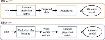
Figure 1: Flowchart illustration of RBoost${}^{\,\text{rank}}$ and RBoost${}^{\,\text{proj}}$.

Many existing multi-class boosting algorithms learn a strong classifier, and a corresponding set of weights, ${\boldsymbol{w}}_{r}\in{\mathbb{R}}^{T}$, for each class $r$. The two novel methods that we propose here, however, learn a single vector of weights, ${\boldsymbol{w}}\in{\mathbb{R}}^{T}$, for all classes. our approaches are conceptually simple and easy to implement. We illustrate our new approaches by incorporating random projections into the boosting framework. Since random projections can be applied to either the original raw data or other intermediate results (for example, weak classifiers’ outputs), we can formulate the multi-class problem as: $1$) a pairwise ranking problem that is based on random projections of the original data; and $2$) a maximum margin problem that is based on random projections of the weak classifiers’ outputs.

In our first approach, we generate a random Gaussian matrix ${\mathbf{P}}\in{\mathbb{R}}^{n\times d}$, whose entry ${\mathbf{P}}(i,j)$ is $\frac{1}{\sqrt{n}}{a_{ij}}$ where $a_{ij}$ is i.i.d. random variables from $\operatorname{\mathcal{N}}(0,1)$. We multiply it with each training instance, ${\boldsymbol{x}}\in{\mathbb{R}}^{d\times 1}$, to obtain a projected data vector, ${\mathbf{P}}{\boldsymbol{x}}\in{\mathbb{R}}^{n\times 1}$. The projected vector, ${\mathbf{P}}{\boldsymbol{x}}$, approximately preserves all pairwise distances of input vector ${\boldsymbol{x}}$, provided that ${\mathbf{P}}$ consists of i.i.d. entries with zero mean and constant variance [11]. In our second approach, we generate a random Gaussian matrix, ${\mathbf{P}}\in{\mathbb{R}}^{n\times T}$. We then multiply it with the output of weak learners, ${\mathbf{P}}[h_{1}(\cdot),h_{2}(\cdot),\cdots,h_{T}(\cdot)]^{\!\top}$, to obtain a new weak learners’ output space, ${\mathbf{P}}H_{i:}^{{\!\top}}\in{\mathbb{R}}^{n\times 1}$. In short, both algorithms rely on the use of random projections to obtain the single-vector parameterized classifier. However, in the first algorithm, the original raw data is randomly projected while in the second algorithm, the weak learners’ outputs are randomly projected. A high-level flowchart that illustrates both approaches is shown in Fig. 1.

III-A Multi-class boosting by randomly projecting the original data

We first formulate the multi-class learning problem as a pairwise ranking problem. The basic idea of our approach is to learn a multi-class classifier from the same instance being projected using $k$ different random projection matrices. We create $k$ pre-defined random projection matrices, ${\mathbf{P}}^{(1)},{\mathbf{P}}^{(2)},\cdots,{\mathbf{P}}^{(k)}$, for each class, where the superscript indicates the class label associated to the random projection matrix. Given a training instance, $({{\boldsymbol{x}}_{i}},{y_{i}})$, the following condition, $F({{\mathbf{P}}^{(y_{i})}}{{\boldsymbol{x}}_{i}})>F({{\mathbf{P}}^{(r)}}{{\boldsymbol{x}}_{i}}),\forall r\neq{y_{i}}$, has to be satisfied. That is to say, the correct model’s response must be larger than all the incorrect models’ responses. We can strengthen this by requiring that the difference $F({{\mathbf{P}}^{(y_{i})}}{{\boldsymbol{x}}_{i}})-F({{\mathbf{P}}^{(r)}}{{\boldsymbol{x}}_{i}})$ is as large as possible. Motivated by the large margin principle, we formulate our multi-class problem in the framework of maximum-margin learning.

Learning using the exponential loss

Given that we have $m$ training samples with $k$ classes, the total number of such pairwise relations is $m(k-1)$. Putting it into the large-margin learning framework, we can define the margin associated with the above condition as, $F({{\mathbf{P}}^{(y_{i})}}{{\boldsymbol{x}}_{i}})-F({{\mathbf{P}}^{(r)}}{{\boldsymbol{x}}_{i}})$, which can be explicitly rewritten as,

$$\rho_{ir} =F({{\mathbf{P}}^{(y_{i})}}{{\boldsymbol{x}}_{i}})-F({{\mathbf{P}}^{(r)}}{{\boldsymbol{x}}_{i}})$$ (1)

$$={\textstyle\sum_{t=1}^{T}}h_{t}({{\mathbf{P}}^{(y_{i})}}{{\boldsymbol{x}}_{i}})w_{t}-{\textstyle\sum_{t=1}^{T}}h_{t}({{\mathbf{P}}^{(r)}}{{\boldsymbol{x}}_{i}})w_{t}$$

$$={\textstyle\sum_{t=1}^{T}}\delta h_{t}({{\mathbf{P}}^{(y_{i})}},{{\mathbf{P}}^{(r)}},{{\boldsymbol{x}}_{i}})w_{t}$$

$$={{\boldsymbol{\delta}}{\boldsymbol{\hbar}}}({{\mathbf{P}}^{(y_{i})}},{{\mathbf{P}}^{(r)}},{{\boldsymbol{x}}_{i}})^{\!\top}{\boldsymbol{w}},$$

where $\delta h_{t}({{\mathbf{P}}^{(y_{i})}},{{\mathbf{P}}^{(r)}},{{\boldsymbol{x}}_{i}})=h_{t}({{\mathbf{P}}^{(y_{i})}}{{\boldsymbol{x}}_{i}})-h_{t}({{\mathbf{P}}^{(r)}}{{\boldsymbol{x}}_{i}})$, and

$${{\boldsymbol{\delta}}{\boldsymbol{\hbar}}}(\cdot,\cdot,\cdot)=\bigl{[}\delta h_{1}(\cdot,\cdot,\cdot),\delta h_{2}(\cdot,\cdot,\cdot),\cdots,\delta h_{T}(\cdot,\cdot,\cdot)\bigr{]}^{\!\top}\in\mathbb{R}^{T\times 1}$$

is a column vector. The purpose is to learn a regularized model that satisfies as many constraints, $\rho_{ir}>0$, as possible. That is to say, we minimize the training error of the model with a controlled capacity. In theory, both of the two proposed boosting methods can employ any convex loss function. We first show how to derive the boosting iteration using the exponential loss. Later we generalize it to any convex loss.

With the exponential loss, the primal problem can be written as,

$$\min_{{\boldsymbol{w}},\boldsymbol{\rho}}\quad \log\bigl{(}\sum\nolimits_{ir}\exp\left(-\rho_{ir}\right)\bigr{)}+\nu{\bf 1}^{{\!\top}}{\boldsymbol{w}}$$ (2)

$$\mathop{\mathrm{s.t.\!\!:}}\nolimits\quad \rho_{ir}={{\boldsymbol{\delta}}{\boldsymbol{\hbar}}}({{\mathbf{P}}^{(y_{i})}},{{\mathbf{P}}^{(r)}},{{\boldsymbol{x}}_{i}})^{\!\top}{\boldsymbol{w}},\forall\,{\rm pair}\,(ir);\,{\boldsymbol{w}}\geq 0,$$

where $(ir)$ represents the joint index through all of the data and all of the classes. Taking the logarithm of the original cost function does not change the nature of the problem as $\log(\cdot)$ is strictly monotonically increasing. This formulation is similar to the binary totally corrective boosting discussed in [9]. Also we have applied the $\ell_{1}$ norm regularization as in [9, 18] to control the model complexity.

If we can solve the optimization problem (2), the learned model can be easily obtained. Unfortunately, the number of weak learners is usually extremely large or even infinite, which corresponds to an extremely or infinite large number of variables ${\boldsymbol{w}}$, it is usually intractable to solve (2) directly. Column generation can be used to approximately solve this problem [9, 18]. We need to derive a meaningful Lagrange dual problem such that column generation can be applied. The Lagrangian is $L=\log(\sum_{ir}\exp(-\rho_{ir}))+\nu{\bf 1}^{\!\top}{\boldsymbol{w}}-{\boldsymbol{u}}^{\!\top}{\boldsymbol{\rho}}+\sum_{ir}u_{ir}{{\boldsymbol{\delta}}{\boldsymbol{\hbar}}}({{\mathbf{P}}^{(y_{i})}},{{\mathbf{P}}^{(r)}},{{\boldsymbol{x}}_{i}})-{\boldsymbol{q}}^{\!\top}{\boldsymbol{w}}.$ with ${\boldsymbol{q}}\geq 0$. The dual problem can be obtained as $\sup_{{\boldsymbol{u}}}\inf_{{\boldsymbol{w}},\boldsymbol{\rho}}L$.

The Lagrange dual problem can be derived as

$$\min_{{\boldsymbol{u}}}\quad {\textstyle\sum_{ir}}u_{ir}\log(u_{ir})$$ (3)

$$\mathop{\mathrm{s.t.\!\!:}}\nolimits\quad {\textstyle\sum_{ir}}u_{ir}{{\boldsymbol{\delta}}{\boldsymbol{\hbar}}}({{\mathbf{P}}^{(y_{i})}},{{\mathbf{P}}^{(r)}},{{\boldsymbol{x}}_{i}})^{\!\top}\leq\nu{\boldsymbol{1}}^{\!\top},\;{\boldsymbol{u}}\geq 0,{\bf 1}^{{\!\top}}{\boldsymbol{u}}=1.$$

As is the case of AdaBoost [9], the dual is a Shannon entropy maximization problem. The objective function of the dual encourages the dual variables, ${\boldsymbol{u}}$, to be uniform. The Karush-Kunh-Tucker (KKT) optimality condition gives the relationship between the optimal primal and dual variables:

$$u_{ir}=\frac{\exp(-\rho_{ir})}{\sum_{ir}\exp(-\rho_{ir})}.$$ (4)

The primal problem can be solved using an efficient Quasi-Newton method like L-BFGS-B, and the dual variables can be obtained using the KKT condition. From the dual, the subproblem for generating weak classifiers is,

$$h^{\ast}(\cdot)=\mathop{\mathrm{argmax}}\limits_{h(\cdot)\in\mathcal{H}}{\sum_{ir}}u_{ir}\delta h({{\mathbf{P}}^{(y_{i})}},{{\mathbf{P}}^{(r)}},{{\boldsymbol{x}}_{i}}).$$ (5)

This corresponds to find the most violated constraint of the dual problem (3). The details of our ranking based multi-class boosting algorithm are given in Algorithm LABEL:ALG:alg1.

Algorithm 1 Column generation based RBoost${}^{\,\text{rank}}$.

Stage-wise boosting

The advantage of the algorithm outlined above is that it is totally corrective in that the primal variables, ${\boldsymbol{w}}$, are updated at each boosting iteration. However, the training of this approach can be expensive when the number of training data and classes are large. In this section, we design a more efficient approach by minimizing the loss function in a stage-wise manner, similar to those derived in AdaBoost. Looking at the primal problem (2), the optimal ${\boldsymbol{w}}$ can be calculated analytically as follows. At iteration $t$, we fix the value of $w_{1}$, $w_{2}$, $\cdots$, $w_{t-1}$. So $w_{t}$ is the only variable to optimize. The primal cost function can then be written as

$$F_{p}=\sum_{ir}Q_{ir}\exp\bigl{(}-\delta h_{t}({{\mathbf{P}}^{(y_{i})}},{{\mathbf{P}}^{(r)}},{{\boldsymbol{x}}_{i}})w_{t}\bigr{)},$$ (6)

where $Q_{ir}=\exp\bigl{(}-\sum_{j=1}^{t-1}\delta h_{j}({{\mathbf{P}}^{(y_{i})}},{{\mathbf{P}}^{(r)}},{{\boldsymbol{x}}_{i}})w_{j}\bigr{)}$. If we use discrete weak learners, $h(\cdot)\in\{-1,+1\}$, then $\delta h_{t}(\cdot)\in\{-2,0,2\}$, and $F_{p}$ can be simplified into:

$$F_{p}={\sum_{\delta h_{t}=0}}Q_{ir} +{\sum_{\delta h_{t}=2}}Q_{ir}\exp(-2w_{t})+{\sum_{\delta h_{t}=-2}}Q_{ir}\exp(2w_{t}).$$ (7)

Let $Q_{+}=\sum_{\delta h_{t}=2}Q_{ir}$ and $Q_{-}=\sum_{\delta h_{t}=-2}Q_{ir}$, then $F_{p}$ is minimized when

$$w_{t}=\frac{1}{4}\log\left(\frac{Q_{+}}{Q_{-}}\right).$$ (8)

When real-valued weak learners are used, with the output in $\left[-1,1\right]$, we can calculate $w_{t}$ by minimizing the upper bound of $F_{p}$ as follows,

$$F_{p}\leq\sum_{ir}Q_{ir}\Bigl{[} 0.5\exp(w_{t})\bigl{(}1-\delta h_{t}({{\mathbf{P}}^{(y_{i})}},{{\mathbf{P}}^{(r)}},{{\boldsymbol{x}}_{i}})\bigr{)}$$

$$+0.5\exp(-w_{t})\bigl{(}1+\delta h_{t}({{\mathbf{P}}^{(y_{i})}},{{\mathbf{P}}^{(r)}},{{\boldsymbol{x}}_{i}})\bigr{)}\Bigr{]}.$$

Here we have used the fact that $\exp(-wh)\leq 0.5\exp(w)(1-h)+0.5\exp(-w)(1+h)$. Similarly $F_{p}$ is minimized when

$$w_{t}=\frac{1}{2}\log\left(\frac{1+b}{1-b}\right),$$ (9)

where $b={\textstyle\sum_{ir}}Q_{ir}\delta h_{t}({{\mathbf{P}}^{(y_{i})}},{{\mathbf{P}}^{(r)}},{{\boldsymbol{x}}_{i}})$. For the stage-wise boosting algorithm, we simply replace Step ④ in Algorithm LABEL:ALG:alg1 with (8) or (9). Note that the formulation of our stage-wise boosting is similar to that of RankBoost proposed by Freund et al. [16]. Besides the efficiency of optimization at each iteration, this stage-wise optimization does not have any parameter to tune. One only needs to determine when to stop. The disadvantage, compared with totally corrective boosting [9], is that it may need more iterations to converge.

General convex loss

The following derivations are based on the important concept of convex conjugate or Fenchel duality from convex optimization.

Definition 1 (Convex Conjugate)

Let $f:\mathbb{R}^{n}\rightarrow\mathbb{R}$. The function $F^{*}:\mathbb{R}^{n}\rightarrow\mathbb{R}$, defined as

$$f^{*}({\boldsymbol{u}})=\sup_{{\boldsymbol{x}}\in{\rm dom}f}[{\boldsymbol{u}}^{\!\top}{\boldsymbol{x}}-f({\boldsymbol{x}})],$$ (10)

is the convex conjugate or Fenchel duality of the function $f(\cdot)$. The domain of the conjugate function consists of ${\boldsymbol{u}}\in\mathbb{R}^{n}$ for which the supremum is finite.

It is easy to verify that $f^{*}(\cdot)$ is always convex since it is the point-wise supremum of a family of affine functions of ${\boldsymbol{u}}$. This holds even if $f(\cdot)$ is not a convex function.

If $f(\cdot)$ is convex and closed, then $f^{**}=f$. For a point-wise loss function, $\lambda(\boldsymbol{\rho})=\sum_{i}\lambda(\rho_{i})$, the convex conjugate of the sum is the sum of the convex conjugates:

$$\lambda^{*}({\boldsymbol{u}})=\sum_{\boldsymbol{\rho}}\left\{{\boldsymbol{u}}^{\!\top}{\boldsymbol{\rho}}-\sum_{i}\lambda(\rho_{i})\right\} =\sum_{i}\sup_{\rho_{i}}\{u_{i}\rho_{i}-\lambda(\rho_{i})\}$$

$$=\sum_{i}\lambda^{*}(u_{i}).$$ (11)

We consider functions of Legendre type here, which means, the gradient $f^{\prime}(\cdot)$ is defined on the domain of $f(\cdot)$ and is an isomorphism between the domains of $f(\cdot)$ and $f^{*}(\cdot)$.

The general $\ell_{1}$-norm regularized optimization problem we want to learn a classifier is

$$\min_{{\boldsymbol{w}},\boldsymbol{\rho}}\; \;\sum_{ir}\lambda(\rho_{ir})+\nu{\bf 1}^{\!\top}{\boldsymbol{w}}$$

$$\mathop{\mathrm{s.t.\!\!:}}\nolimits\; \rho_{ir}={{\boldsymbol{\delta}}{\boldsymbol{\hbar}}}({\mathbf{P}}^{(y_{i})},{\mathbf{P}}^{(r)},{\boldsymbol{x}}_{i})^{\!\top}{\boldsymbol{w}},{\boldsymbol{w}}\geq 0.$$ (12)

Here $\lambda(\cdot)$ is a convex surrogate of the zero-one loss, e.g., the exponential loss, logistic regression loss. We assume that $\lambda(\cdot)$ is smooth.

Although the variable of interest is ${\boldsymbol{w}}$, we need to keep the auxiliary variable $\boldsymbol{\rho}$ in order to derive a meaningful dual problem. The Lagrangian is

$$L =\sum_{ir}\lambda(\rho_{ir})+\nu{\bf 1}^{\!\top}{\boldsymbol{w}}$$

$$\quad-\sum_{ir}u_{ir}(\rho_{ir}-{{\boldsymbol{\delta}}{\boldsymbol{\hbar}}}({\mathbf{P}}^{(y_{i})},{\mathbf{P}}^{(r)},{\boldsymbol{x}}_{i})^{\!\top}{\boldsymbol{w}})-{\boldsymbol{q}}^{\!\top}{\boldsymbol{w}}$$

$$=\Bigl{[}\nu{\bf 1}^{\!\top}+\sum_{ir}u_{ir}{{\boldsymbol{\delta}}{\boldsymbol{\hbar}}}({\mathbf{P}}^{(y_{i})},{\mathbf{P}}^{(r)},{\boldsymbol{x}}_{i})^{\!\top}-{\boldsymbol{q}}\Bigr{]}{\boldsymbol{w}}$$

$$\quad-\left[\sum_{ir}u_{ir}\rho_{ir}-\sum_{ir}\lambda(\rho_{ir})\right].$$

In order for $L$ to have finite infimum over the primal variables, the first term of $L$ must be zero, which leads to

$$\nu{\bf 1}^{\!\top}+\sum_{ir}u_{ir}{{\boldsymbol{\delta}}{\boldsymbol{\hbar}}}({\mathbf{P}}^{(y_{i})},{\mathbf{P}}^{(r)},{\boldsymbol{x}}_{i})^{\!\top}\geq 0.$$ (13)

The infimum of the second term of $L$ is $-\sum_{ir}\lambda^{*}(u_{ir})$ by using (10) and (11). Therefore the Lagrange dual problem of (III-A) is

$$\max_{{\boldsymbol{u}}}\; \;-\sum_{ir}\lambda^{*}(u_{ir}),\;\,\mathop{\mathrm{s.t.\!\!:}}\nolimits\,\eqref{EQ:App10}.$$ (14)

We can reverse the sign of the dual variable ${\boldsymbol{u}}$ and rewrite (14) into its equivalent form

$$\min_{{\boldsymbol{u}}}\; \;\sum_{ir}\lambda^{*}(-u_{ir})$$

$$\mathop{\mathrm{s.t.\!\!:}}\nolimits\; \sum_{ir}u_{ir}{{\boldsymbol{\delta}}{\boldsymbol{\hbar}}}({\mathbf{P}}^{(y_{i})},{\mathbf{P}}^{(r)},{\boldsymbol{x}}_{i})^{\!\top}\leq\nu{\bf 1}^{\!\top}.$$ (15)

The KKT condition between the primal (III-A) and the dual (III-A) shows the relation of the primal and dual variables

$$u_{ir}=-\lambda^{\prime}(\rho_{ir}),$$ (16)

which holds at optimality. The dual variable ${\boldsymbol{u}}$ is the negative gradient of the loss at $\rho_{ir}$. This can be obtained by setting the first derivative of $L$ to be zeros. Under the assumption that both the primal and dual problems are feasible and the Slater’s condition satisfies, strong duality holds between the primal and dual problems.

We need to use column generation to approximately solve the original problem because the dimension of the primal variable ${\boldsymbol{w}}$ can be extremely large or infinite. The high-level idea of column generation is to only consider a small subset of the variables in the primal; i.e., only a subset of ${\boldsymbol{w}}$ is considered. The problem solved using this subset is called the restricted master problem (RMP). It is well known that each primal variable corresponds to a constraints in the dual problem. Solving RMP is equivalent to solving a relaxed version of the dual problem. With a finite ${\boldsymbol{w}}$, the set of constraints in the dual problem are finite, and we can solve the dual problem such that it satisfies all the existing constraints. If we can prove that among all the constraints that we have not added to the dual problem, no single constraint is violated, then we can draw the conclusion that solving the restricted problem is equivalent to solving the original problem. Otherwise, there exists at least one constraint that is violated. The violated constraints correspond to variables in primal that are not in RMP. Adding these variables to RMP leads to a new RMP that needs to be re-optimized. To speed up convergence, one typically finds the most violated constraint in the dual by solving the following problem, according to the constraint in (III-A):

$$\max_{h(\cdot)}\sum_{ir}u_{ir}\delta h({{\mathbf{P}}^{(y_{i})}},{{\mathbf{P}}^{(r)}},{{\boldsymbol{x}}_{i}}).$$ (17)

We only need to change the primal and dual problems involved in Algorithm LABEL:ALG:alg1 to obtain the column generation based multi-class random boosting with a general convex loss function. Specifically, only two lines need a change in Algorithm LABEL:ALG:alg1 and the rest remains identical:

Step ④: Solve the primal problem (III-A), or the dual problem (III-A);

Step ⑤: If the primal problem is solved, update the dual variable ${\boldsymbol{u}}$ using (16).

Note that the derivation of the dual problem (3) also follows the above analysis (using the fact that the convex conjugate of the log-sum-exp function is the Shannon entropy). Mathematically the convex conjugate of $f({\boldsymbol{x}})=\log(\sum_{i}x_{i})$ is $f^{*}({\boldsymbol{u}})=\sum_{i}u_{i}\log u_{i},$ if ${\boldsymbol{u}}\geq 0$ and $\sum_{i}u_{i}=1$; otherwise $f^{*}({\boldsymbol{u}})=\infty$.

III-B Multi-class boosting by randomly projecting weak classifiers’ outputs

In contrast to the approach proposed in the previous section, where we randomly project the original data to new spaces, we can also randomly project the output of weak classifiers, ${\mathbf{H}}$, to new spaces. Our intuition is that if ${\mathbf{H}}$ is linearly separable then the randomly projected data, ${\mathbf{P}}{\mathbf{H}}^{{\!\top}}$, is likely to be linearly separable as well, as long as the random projection matrices satisfy some mild assumptions [13]. As in the previous approach, we learn a multi-class classifier based on pairwise comparisons. We create $k$ pre-defined random projection matrices, ${\mathbf{P}}^{(1)},{\mathbf{P}}^{(2)},\cdots,{\mathbf{P}}^{(k)}$, one for each class. Given a training instance $({{\boldsymbol{x}}_{i}},{y_{i}})$ and the weak classifiers’ responses, $H_{i:}$, the condition ${{\mathbf{P}}^{(y_{i})}}H_{i:}^{{\!\top}}{\boldsymbol{w}}>{{\mathbf{P}}^{(r)}}H_{i:}^{{\!\top}}{\boldsymbol{w}},\forall r\neq{y_{i}}$ has to be satisfied. The intuition is the same as in the previous case: the correct model’s response should be larger than all the incorrect models’ responses. Note that in this approach, ${\boldsymbol{w}}\in{\mathbb{R}}^{n}$, i.e., it has a fixed size and is independent of the number of boosting iterations (as compared to the previous approach where the size of ${\boldsymbol{w}}$ is equal to the number of boosting iterations, ${\boldsymbol{w}}\in{\mathbb{R}}^{T}$). We define a margin associated with the above condition as $\rho_{ir}={{\mathbf{P}}^{(y_{i})}}H_{i:}^{{\!\top}}{\boldsymbol{w}}-{{\mathbf{P}}^{(r)}}H_{i:}^{{\!\top}}{\boldsymbol{w}}$. Now the margin has been defined, and the learning can be solved within the large-margin framework, as described in the previous section. We now apply the logistic loss due to its robustness in handling noisy data [28]. Again, any other convex surrogate loss can be used. Since the projected space, ${\mathbf{P}}{\mathbf{H}}^{{\!\top}}$, can also be much larger than the original space, ${\mathbf{H}}$, we expect that some projected features might turn out to be irrelevant. We also apply the $\ell_{1}$-norm regularization as in [9], resulting in the following learning problem:

$$\min_{{\boldsymbol{w}},{\boldsymbol{\rho}}}\quad \frac{1}{mk}\sum_{i=1}^{m}\sum_{r=1}^{k}\log\bigl{(}1+\exp\left(-\rho_{ir}\right)\bigr{)}+\nu{\boldsymbol{1}}^{\!\top}{\boldsymbol{w}}$$ (18)

$$\mathop{\mathrm{s.t.\!\!:}}\nolimits\quad \rho_{ir}={{\mathbf{P}}^{(y_{i})}}H_{i:}^{{\!\top}}{\boldsymbol{w}}-{{\mathbf{P}}^{(r)}}H_{i:}^{{\!\top}}{\boldsymbol{w}},\forall i,\forall r;\quad{\boldsymbol{w}}\geq 0.$$

Note that ${\boldsymbol{w}}\geq 0$ enforces the non-negative constraint on ${\boldsymbol{w}}$. The Lagrangian of (18) can be written as

$$L= \frac{1}{mk}\sum_{i,r}\log\bigl{(}1+\exp\left(-\rho_{ir}\right)\bigr{)}+\nu{\boldsymbol{1}}^{\!\top}{\boldsymbol{w}}$$ (19)

$$-\sum_{i,r}u_{ir}(\rho_{ir}-{{\mathbf{P}}^{(y_{i})}}H_{i:}^{{\!\top}}{\boldsymbol{w}}+{{\mathbf{P}}^{(r)}}H_{i:}^{{\!\top}}{\boldsymbol{w}}-{\boldsymbol{p}}^{{\!\top}}{\boldsymbol{w}}),$$

with ${\boldsymbol{u}}\geq 0$ and ${\boldsymbol{p}}\geq 0$. At optimum, the first derivative of the Lagrangian w.r.t. the primal variables, ${\boldsymbol{w}}$, must be zeros,

$$\frac{\partial L}{\partial{\boldsymbol{w}}}={\bf 0} \rightarrow\sum_{i,r}u_{ir}\left({{\mathbf{P}}^{(y_{i})}}-{{\mathbf{P}}^{(r)}}\right)H_{i:}^{{\!\top}}={\boldsymbol{p}}^{{\!\top}}-\nu{\bf 1}^{{\!\top}}$$ (20)

$$\rightarrow\sum_{i,r}u_{ir}\boldsymbol{\delta}{\mathbf{P}}(y_{i},r)H_{i:}^{{\!\top}}={\boldsymbol{p}}^{{\!\top}}-\nu{\bf 1}^{{\!\top}},$$

where $\boldsymbol{\delta}{\mathbf{P}}(y_{i},r)={{\mathbf{P}}^{(y_{i})}}-{{\mathbf{P}}^{(r)}}$. By taking the infimum over the primal variables, $\rho_{ir}$,

$$\frac{\partial L}{\partial\rho_{ir}}=0\rightarrow\rho_{ir}=-\log\left(\frac{-mku_{ir}}{mku_{ir}-1}\right),\forall i,\forall r,$$ (21)

and

$$\inf_{\rho_{ir}}L= \frac{1}{mk}\sum_{i,r}\Bigl{[}-(1+mku_{ir})\log\left(1+mku_{ir}\right)$$ (22)

$$-mku_{ir}\log\left(-mku_{ir}\right)\Bigr{]}.$$

Reversing the sign of ${\boldsymbol{u}}$, the Lagrange dual can be written as

$$\max_{{\boldsymbol{u}}}\quad -\frac{1}{mk}\sum_{i=1}^{m}\sum_{r=1}^{k}\Bigl{[}mku_{ir}\log\left(mku_{ir}\right)+$$ (23)

$$\qquad\left(1-mku_{ir}\right)\log\left(1-mku_{ir}\right)\Bigr{]}$$

$$\mathop{\mathrm{s.t.\!\!:}}\nolimits\quad \sum_{i,r}u_{ir}\boldsymbol{\delta}{\mathbf{P}}(y_{i},r)H_{i:}^{{\!\top}}<\nu{\bf 1}^{{\!\top}}.$$

Note that here the number of constraints is equal to the size of the new space ($n$). At each iteration, we choose the weak learner, $h_{t}(\cdot)$, that most violates the dual constraint in (23). The subproblem of generating the weak classifier at iteration $t$ can then be expressed as:

$$h^{\ast}(\cdot)=\mathop{\mathrm{argmax}}\limits_{h(\cdot),v}\;\sum_{i,r}u_{ir}\left[H_{i,1:t-1},h({{\boldsymbol{x}}_{i}})\right]\boldsymbol{\delta}{{\boldsymbol{p}}}(y_{i},r;v),$$ (24)

$v=1,\ldots,n,\,\,\forall h(\cdot)\in\mathcal{H}$ and

$$\boldsymbol{\delta}{{\boldsymbol{p}}}(y_{i},r;v)=\left[P^{(y_{i})}_{v1}-P^{(r)}_{v1},\cdots,P^{(y_{i})}_{vt}-P^{(r)}_{vt}\right]^{\!\top}\in{\mathbb{R}}^{T\times 1}.$$

Here a significant difference compared with conventional boosting is that the selection of the current best weak classifier depends on all previously selected weak classifiers.

The idea behind our approach is that performance improves as more weak classifiers, $h(\cdot)$, are added to the constraint. This process can continue as long as there exists at least one constraint that is violated, i.e.,

$$\max\left({\textstyle\sum}_{i,r}U_{ir}\boldsymbol{\delta}{\mathbf{P}}(y_{i},r)H_{i,1:t}^{{\!\top}}\right)<\nu+\epsilon,$$

or when adding an additional weak classifiers ceases to have a significant impact on the objective value of (18), i.e., $\left|\frac{{\rm Opt}_{t-1}-{\rm Opt}_{t}}{{\rm Opt}_{t-1}}\right|<\epsilon$. In our experiments we use the latter as our stopping criterion. Through the KKT optimality condition, the gradient of Lagrangian (19) over primal variables, ${\boldsymbol{\rho}}$, and dual variables, ${\boldsymbol{u}}$, must vanish at the optimum. The relationship between the optimal value of ${\boldsymbol{\rho}}$ and ${\boldsymbol{u}}$ can be expressed as

$$u_{ir}=\frac{\exp(-\rho_{ir})}{mk\bigl{(}1+\exp(-\rho_{ir})\bigr{)}}.$$ (25)

The details of our random projection based multi-class boosting algorithm are given in Algorithm LABEL:ALG:alg2.

Algorithm 2 Column generation based RBoost${}^{\,\text{proj}}$.

The use of general convex loss here follows the similar generalization procedure as shown in the previous section.

	RBoost${}^{\,\text{rank}}$	RBoost${}^{\,\text{proj}}$
Pre-processing step for decision stumps	$O\bigl{(}nmk\log(mk)\bigr{)}$	$O(dm\log m)$
At each iteration
Train the weak learner (decision stump)	$O(nmk)$	$O(nmk+nmd)$
Solve the optimization problem (RBoost)	$O(mk)$	$O(n^{3})$
Total computational complexity	$O\bigl{(}nmk\log(mk)+nmkT\bigr{)}$	$O\bigl{(}dm\log m+nm(k+d)T+n^{3}T\bigr{)}$

TABLE I: Computational complexity of RBoost. $m$ is the number of training samples. $n$ is the number of projected dimensions. $k$ is the number of classes. $d$ is the dimension size of the original data. $T$ is the number of iterations. Note that weak classifier training (learning decision stumps) take up most of the computation time for both methods.

III-C Computational complexity

We analyze the complexity of our new approaches in this section. For the sake of completeness, we also analyze the computational complexity of training weak classifiers. For simplicity, we use a decision stump as our weak classifier. Note that any weak classifier algorithms can be applied here. For fast training of decision stumps, we first sort feature values and cache sorted results in memory. At each boosting iteration, all decision stumps’ thresholds will be searched and the optimal decision stump $h^{\ast}(\cdot)$, which satisfies (5) or (24), will be saved as the weak learner for the $t$-iteration. For RBoost${}^{\,\text{rank}}$ (Algorithm LABEL:ALG:alg1), the total number of pairwise relationships is $m(k-1)$. We first sort features in each projected dimension. This pre-processing step requires $O\bigl{(}nmk\log(mk)\bigr{)}$ for sorting $n$ dimensions. In Step ①  we train decision stumps for each projected dimension. Step ① takes $O(nmk)$. Step ④ can simply be ignored since it can be solved efficiently using (8) or (9). Let the maximum number of iterations be $T$, the time complexity is $O(nmkT)$. The total time complexity for RBoost${}^{\,\text{rank}}$ is $O\bigl{(}nmk\log(mk)+nmkT\bigr{)}$.

For RBoost${}^{\,\text{proj}}$ (Algorithm LABEL:ALG:alg2), the time required to sort $d$ features is $O(dm\log m)$. Step ① finds the optimal weak learner that satisfies (24). The multiplication, $u_{ir}\boldsymbol{\delta}{{\boldsymbol{p}}}(y_{i},r;v)$, in (24) takes $O(nmk)$ for all $n$ dimensions. Training decision stumps requires $O(nmd)$. Hence, Step ① requires $O(nmk+nmd)$. In Step ④  we solve $n$ variables at each iteration. Let us assume the computational complexity of L-BFGS-B is roughly cubic. Hence, the time complexity for $T$ boosting iterations is $O\bigl{(}nm(k+d)T+n^{3}T\bigr{)}$ and the total time complexity for RBoost${}^{\,\text{proj}}$ is $O\bigl{(}dm\log m+nm(k+d)T+n^{3}T\bigr{)}$. The computational complexity of both approaches is summarized in Table I. Note that weak classifier training (learning decision stumps) take up most of the computation time for both methods.

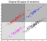
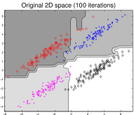
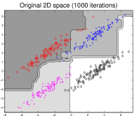
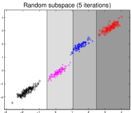
Figure 2: Decision boundaries on the artificial data set. First $3$ columns: Classification of four diagonal distributions on the original two dimensional space at $5$, $100$ and $1000$ boosting iterations. Last column: Classification on randomly projected subspace (selectively chosen to illustrate a better separation between classes).

III-D Discussion

Advantage of applying random projections

One possible advantage of applying random projections is that random projections may further increase class separation on some data sets. We illustrate this in the following toy example. We generate an artificial data set with four diagonal distributions. Each diagonal distribution is randomly generated from the multivariate normal distribution with covariance, $\left[2.5,1.5;1.5,1\right]$ and mean $\left[-3,2\right]$, $\left[-3,-2\right]$, $\left[3,4\right]$, $\left[3,0\right]$. We train a one-versus-all boosting (with the decision stump as the weak learner) and plot the decision boundary at $5$, $100$ and $1000$ boosting iterations. We also randomly project the artificial data to the new $2$D space and train the one-versus-all boosting classifier. Decision boundaries of different examples are shown in Fig. 2. From the figure, classification on the randomly projected subspace (Fig. 2: last column) clearly indicates its advantage compared to classification on the original space.

Theoretical justification based on margin analysis

In this section we justify the use of random projections on the proposed single-model multi-class classifier. We begin by defining the margin on MultiBoost [27] and its bound when the weak classifiers’ response, ${\mathbf{H}}$, is randomly projected to the new space with a random projection matrix, ${\mathbf{P}}$.

Definition 2 (Multi-class Margin for Boosting)

Given a data set, $S=\{({{\boldsymbol{x}}_{i}}\in\mathbb{R}^{d},y_{i}\in\operatorname{\mathcal{Y}}=\{1,\cdots,k\})\}_{i=1}^{m}$, the weak learners’ response on the training data, ${\mathbf{H}}$, and weak learners’ coefficients, ${\mathbf{W}}=\left[{\boldsymbol{w}}_{1}^{\!\top},\cdots{\boldsymbol{w}}_{k}^{\!\top}\right]$ where ${\boldsymbol{w}}_{r}\in\mathbb{R}^{T}$ is weak learners’ coefficients for class $r$. The margin for boosting can be defined as,

$$\gamma=\min_{({\boldsymbol{x}},y)\in S}\Big{(}\frac{\left\langle{\boldsymbol{w}}_{y},{\mathbf{H}}({\boldsymbol{x}})\right\rangle}{\|{\boldsymbol{w}}_{y}\|\|{\mathbf{H}}({\boldsymbol{x}})\|}-\max_{y^{\prime}\neq y}\frac{\left\langle{\boldsymbol{w}}_{y^{\prime}},{\mathbf{H}}({\boldsymbol{x}})\right\rangle}{\|{\boldsymbol{w}}_{y^{\prime}}\|\|{\mathbf{H}}({\boldsymbol{x}})\|}\Big{)}.$$

Theorem 1 (Margin Preservation)

If the boosting has margin $\gamma$, then for any $\delta,\epsilon\in(0,1)$ and any

$$n>\frac{12}{3\epsilon^{2}-2\epsilon^{3}}\ln\frac{6km}{\delta},$$

with probability at least $1-\delta$, the boosting associated with projected weak learners’ coefficients, ${\mathbf{P}}{\boldsymbol{w}}_{r},\forall r$, and the projected weak learners’ response, ${\mathbf{P}}{\mathbf{H}}$, has margin no less than

$$-\frac{1+3\epsilon}{1-\epsilon^{2}}+\frac{\sqrt{1-\epsilon^{2}}}{1+\epsilon}+\frac{1+\epsilon}{1-\epsilon}\gamma.$$

The above theorem shows that the multi-class margin can be well preserved after both weak learner’s coefficients, ${\mathbf{W}}$, and weak learners’ responses, ${\mathbf{H}}$, are randomly projected. This theorem justifies the use of random projection on MultiBoost [27]. The next theorem defines margin separability for the proposed single-vector parameterized multi-class boosting.

Theorem 2 (Single-vector Multi-class Boosting)

Given any random Gaussian matrix ${\mathbf{R}}\in\mathbb{R}^{n\times kT}$, whose entry ${\mathbf{R}}(i,j)=$ $\frac{1}{\sqrt{n}}{a_{ij}}$ where $a_{ij}$ is i.i.d. random variables from $\operatorname{\mathcal{N}}(0,1)$. Denote ${\mathbf{P}}_{y}\in\mathbb{R}^{n,T}$ as the $y$-th submatrix of ${\mathbf{R}}$, that is ${\mathbf{R}}=[{\mathbf{P}}_{1},$ $\cdots,{\mathbf{P}}_{r},$ $\cdots,$ ${\mathbf{P}}_{k}]$. If the boosting has margin $\gamma$, then for any $\delta,\epsilon\in(0,1]$ and any

$$n>\frac{12}{3\epsilon^{2}-2\epsilon^{3}}\ln{\frac{6m(k-1)}{\delta}},$$

there exists a single-vector ${\boldsymbol{v}}\in\mathbb{R}^{n}$, such that

$$\Pr\Big{(} \frac{\left\langle{\boldsymbol{v}},{\mathbf{P}}_{y}{\mathbf{H}}({\boldsymbol{x}})\right\rangle-\left\langle{\boldsymbol{v}},{\mathbf{P}}_{y^{\prime}}{\mathbf{H}}({\boldsymbol{x}})\right\rangle}{\|{\boldsymbol{v}}\|\sqrt{\|{\mathbf{P}}_{y}{\mathbf{H}}({\boldsymbol{x}})\|^{2}+\|{\mathbf{P}}_{y^{\prime}}{\mathbf{H}}({\boldsymbol{x}})\|^{2}}}\geq$$

$$\frac{-2\epsilon}{1-\epsilon}+\frac{1+\epsilon}{{\sqrt{2k}}(1-\epsilon)}\gamma\Big{)}\geq 1-\delta,\quad\quad\forall y^{\prime}\neq y.$$ (26)

The above theorem reveals that there exists a single-vector ${\boldsymbol{v}}\in\mathbb{R}^{n}$ under which the margin is preserved up to an order of $O(\gamma/\sqrt{2k})$. In other words, the multi-class margin can be well preserved after random projection as long as the newly projected dimension, $n$, satisfies some mild condition. Not only the theorem justifies the use of random projection to learn the single-model classifier, it also shows that the projected dimensions, $n$, only grows logarithmically with the number of classes, $k$. This finding is important for problems where the number of classes is large. Note that Theorem 2 only applies to the second approach presented in this work.

IV Experiments

We evaluate our approaches on artificial, machine learning and visual recognition data sets and compare our approaches against existing multi-class boosting algorithms. For AdaBoost.ECC, we perform binary partitioning at each iteration using the random-half method [30]. Decision stumps are used as the weak classifier for all boosting algorithms.

Data                    Ada.ECC                   Ada.MH                   Ada.MO               MultiBoost${}^{\ell_{1}}$               RBoost${}^{\,\text{rank}}$              RBoost${}^{\,\text{proj}}$

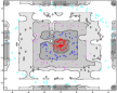
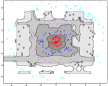
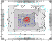
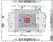
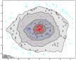
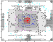
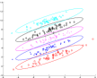
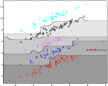
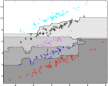
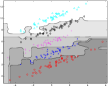
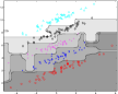
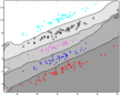
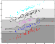
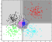
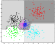
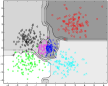
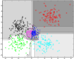
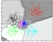
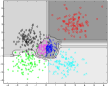
Figure 3: Decision boundaries of various multi-class boosting algorithms on artificial data sets. The data distribution is shown in the first column. The number of boosting iterations is set to $500$.

IV-A Toy data

We first illustrate the behavior of our algorithms on artificial multi-class data sets. We consider the problem of discriminating various object classes on a $2$D plane. For this experiment the feature vectors are the $xy$-coordinates of the $2$D plane. We train $6$ different classifiers using AdaBoost.ECC [7], AdaBoost.MH [26], AdaBoost.MO [26], MultiBoost [27], and our proposed RBoost${}^{\,\text{rank}}$ and RBoost${}^{\,\text{proj}}$. For MultiBoost, we use hinge loss and choose the regularization parameter from $\{10^{-4},$ $10^{-3},$ $10^{-2}\}$. For both RBoost${}^{\,\text{rank}}$ and RBoost${}^{\,\text{proj}}$, we set $n$ to be equal to $500$. For RBoost${}^{\,\text{proj}}$, we choose the regularization parameter, $\nu$, from $\{10^{-7},$ $10^{-6},$ $10^{-5},$ $10^{-4},$ $10^{-3}\}$. In this experiment, we set the number of boosting iterations to $500$. Fig. 3 plots decision boundaries of various methods. On two dimensional toy data sets, we observe that decision boundaries of RBoost${}^{\,\text{rank}}$ are very similar to the true decision boundary. This is not surprising since all toy data sets are generated from the multivariate normal distribution. Hence, RBoost${}^{\,\text{rank}}$ produces very accurate decision boundaries.

	RBoost${}^{\,\text{rank}}$				RBoost${}^{\,\text{proj}}$
Data set	$n=1000$	$2500$	$5000$	$10000$	$n=250$	$500$	$1000$	$2000$
Synthetic 1	$3.4$ ($1.5$)	$2.6$ ($0.9$)	$2.1$ ($0.9$)	$1.8$ ($1.5$)	$11.2$ ($1.9$)	$13.0$ ($1.6$)	$11.2$ ($1.3$)	$10.9$ ($2.1$)
Synthetic 2	$0.6$ ($0.6$)	$0.6$ ($0.4$)	$0.2$ ($0.4$)	$0.5$ ($1.1$)	$7.0$ ($2.3$)	$8.2$ ($1.4$)	$6.6$ ($2.2$)	$7.0$ ($1.3$)
Synthetic 3	$3.7$ ($1.2$)	$3.3$ ($1.4$)	$4.0$ ($1.3$)	$3.5$ ($1.3$)	$6.5$ ($2.0$)	$6.9$ ($2.0$)	$6.4$ ($1.8$)	$7.1$ ($2.9$)

TABLE II: Average test errors and standard deviations (shown in $\%$) for different values of $n$. All experiments are repeated $5$ times

Size of the projected space

We use three previous artificial data sets and vary the size of the projected space, $n$. Each data set is randomly split into two groups: $75\%$ for training and the rest for evaluation. We set the maximum number of boosting iterations to $500$. We vary $n$ from $1000$ to $10,000$ for RBoost${}^{\,\text{rank}}$ and $250$ to $2000$ for RBoost${}^{\,\text{proj}}$. For RBoost${}^{\,\text{rank}}$, the larger the parameter $n$, the more features that the algorithm can choose during training. From Theorem 1, as long as $D$ is approximately larger than $\log(mk)$, the margin is preserved with high probability for RBoost${}^{\,\text{proj}}$. Table II reports final classification errors of various $n$. For RBoost${}^{\,\text{rank}}$, we observe a slight increase in generalization performance when $n$ increases. For RBoost${}^{\,\text{proj}}$, as long as $n$ is sufficiently large ($>250$ in this experiment), the final performance is almost not affected by the value of $n$.

	Exponential loss (TC)		Logistic loss (TC)		Exponential loss (SW)
Data set	Test error	CPU time	Test error	CPU time	Test error	CPU time
australian	$\mathbf{14.9}$ ($\mathbf{2.5}$)	$11.7$	$17.4$ ($2.6$)	$6.3$	$15.8$ ($2.1$)	$\mathbf{0.03}$
heart	$\mathbf{19.9}$ ($\mathbf{4.5}$)	$6.5$	$22.7$ ($3.8$)	$1.9$	$21.3$ ($4.2$)	$\mathbf{0.02}$
wine	$3.0$ ($2.4$)	$13.7$	$\mathbf{2.5}$ ($\mathbf{2.3}$)	$1.4$	$2.5$ ($2.7$)	$\mathbf{0.03}$
glass	$34.9$ ($6.1$)	$10.6$	$\mathbf{30.4}$ ($\mathbf{5.2}$)	$4.8$	$31.3$ ($6.2$)	$\mathbf{0.03}$
segment	$\mathbf{3.0}$ ($\mathbf{0.6}$)	$145$	$3.1$ ($0.7$)	$45.2$	$3.3$ ($0.6$)	$\mathbf{0.09}$

TABLE III: Average test errors (in %) and CPU time (seconds) (time taken to solve the optimization problem in step ④  Algorithm LABEL:ALG:alg1). TC: totally-corrective RBoost${}^{\,\text{rank}}$ and SW: stage-wise RBoost${}^{\,\text{rank}}$

IV-B Totally-corrective RBoost${}^{\,\text{rank}}$ and stage-wise RBoost${}^{\,\text{rank}}$

In this experiment, we compare the performance of totally-corrective RBoost${}^{\,\text{rank}}$ with stage-wise RBoost${}^{\,\text{rank}}$. We use UCI machine learning repository data sets and randomly split the data sets into two groups: $75\%$ of samples for training and the rest for evaluation. We set the maximum number of boosting iterations to $500$. We conduct an experiment on two convex losses: the exponential loss and the logistic loss. For totally-corrective boosting, we solve the optimization problem, step ④ in Algorithm LABEL:ALG:alg1, using L-BFGS-B. For L-BFGS-B parameters, we set the maximum number of iterations to $100$, the accuracy of the line search to $10^{-5}$, the convergence parameter to terminate the program to $10^{7}\cdot\epsilon$ (where $\epsilon$ is a machine precision) and the number of corrections to approximate the inverse hessian matrix to $5$. We use the same L-BFGS-B parameters for all experiments. The regularization parameter in (III-A), $\nu$, is determined by $5$-fold cross validation. We choose the best $\nu$ from $\{10^{-7}$, $10^{-6}$, $10^{-5}$, $10^{-4}$, $10^{-3}$, $10^{-2}\}$. For stage-wise RBoost${}^{\,\text{rank}}$, we set $n$ to be $100$ times the dimension size of the original data. All experiments are repeated $10$ times and the average and standard deviation of test errors are reported in Table III. We observe that the performance of both convex losses are comparable and stage-wise RBoost${}^{\,\text{rank}}$ produces comparable test accuracy to totally-corrective RBoost${}^{\,\text{rank}}$. However, stage-wise RBoost${}^{\,\text{rank}}$ has a much lower CPU time. Since both totally-corrective and stage-wise RBoost${}^{\,\text{rank}}$ are comparable, we use stage-wise RBoost${}^{\,\text{rank}}$ in the rest of our experiments.

IV-C UCI data sets

	AdaBoost			RBoost${}^{\,\text{rank}}$			RBoost${}^{\,\text{proj}}$
Data set	Test $50$	Test $100$	Test $1000$	Test $50$	Test $100$	Test $1000$	Test $50$	Test $100$	Test $1000$
australian	$14.8$ ($2.9$)	$14.8$ ($2.1$)	$16.6$ ($2.1$)	$15.3$ ($2.8$)	$15.7$ ($2.2$)	$16.9$ ($2.6$)	$\mathbf{14.2}$ ($\mathbf{2.4}$)	$\mathbf{14.2}$ ($\mathbf{2.4}$)	$\mathbf{14.2}$ ($\mathbf{2.4}$)
b-cancer	$4.3$ ($1.2$)	$4.4$ ($1.1$)	$4.6$ ($1.3$)	$4.6$ ($1.4$)	$4.2$ ($1.3$)	$4.3$ ($1.4$)	$\mathbf{3.9}$ ($\mathbf{1.0}$)	$\mathbf{4.0}$ ($\mathbf{1.0}$)	$\mathbf{4.1}$ ($\mathbf{1.0}$)
c-cancer	$20.0$ ($7.7$)	$18.7$ ($8.8$)	$16.0$ ($9.0$)	$\mathbf{16.7}$ ($\mathbf{7.9}$)	$\mathbf{15.3}$ ($\mathbf{8.3}$)	$\mathbf{16.0}$ ($\mathbf{7.8}$)	$23.3$ ($11.9$)	$23.3$ ($11.9$)	$23.3$ ($11.9$)
diabetes	$26.7$ ($2.1$)	$26.3$ ($3.0$)	$25.7$ ($2.9$)	$25.7$ ($1.5$)	$\mathbf{25.5}$ ($\mathbf{1.3}$)	$26.4$ ($2.6$)	$\mathbf{25.5}$ ($\mathbf{2.2}$)	$25.7$ ($2.1$)	$\mathbf{25.7}$ ($\mathbf{2.1}$)
german	$\mathbf{24.2}$ ($\mathbf{2.3}$)	$24.4$ ($2.3$)	$25.8$ ($3.0$)	$24.6$ ($2.5$)	$\mathbf{24.2}$ ($\mathbf{2.9}$)	$24.9$ ($3.1$)	$24.5$ ($1.6$)	$24.5$ ($1.6$)	$\mathbf{24.5}$ ($\mathbf{1.6}$)
heart	$\mathbf{16.7}$ ($\mathbf{3.1}$)	$17.6$ ($3.4$)	$20.9$ ($3.1$)	$16.9$ ($3.9$)	$\mathbf{16.7}$ ($\mathbf{4.0}$)	$\mathbf{17.6}$ ($\mathbf{3.5}$)	$19.6$ ($2.2$)	$19.9$ ($1.9$)	$19.9$ ($1.9$)
ionosphere	$11.7$ ($2.2$)	$11.6$ ($2.4$)	$10.0$ ($2.8$)	$\mathbf{9.4}$ ($\mathbf{3.1}$)	$\mathbf{7.5}$ ($\mathbf{2.9}$)	$\mathbf{7.4}$ ($\mathbf{3.6}$)	$12.2$ ($3.2$)	$11.9$ ($3.3$)	$12.0$ ($3.3$)
liver	$\mathbf{27.9}$ ($\mathbf{6.3}$)	$\mathbf{28.0}$ ($\mathbf{4.6}$)	$\mathbf{28.4}$ ($\mathbf{3.7}$)	$30.6$ ($4.7$)	$30.5$ ($4.6$)	$30.6$ ($3.6$)	$29.9$ ($5.6$)	$30.0$ ($5.4$)	$30.0$ ($5.4$)
mushrooms	$0.2$ ($0.1$)	$\mathbf{0.0}$ ($\mathbf{0.0}$)	$\mathbf{0.0}$ ($\mathbf{0.0}$)	$0.1$ ($0.1$)	$\mathbf{0.0}$ ($\mathbf{0.0}$)	$\mathbf{0.0}$ ($\mathbf{0.0}$)	$\mathbf{0.0}$ ($\mathbf{0.0}$)	$\mathbf{0.0}$ ($\mathbf{0.0}$)	$\mathbf{0.0}$ ($\mathbf{0.0}$)
sonar	$\mathbf{17.9}$ ($\mathbf{4.3}$)	$\mathbf{16.9}$ ($\mathbf{3.8}$)	$\mathbf{16.5}$ ($\mathbf{2.9}$)	$22.5$ ($5.4$)	$19.8$ ($6.1$)	$18.8$ ($4.7$)	$21.7$ ($4.9$)	$18.5$ ($4.0$)	$19.0$ ($4.5$)
splice	$8.7$ ($0.8$)	$8.4$ ($1.1$)	$8.7$ ($1.3$)	$16.5$ ($1.6$)	$15.1$ ($1.6$)	$11.3$ ($1.3$)	$\mathbf{8.3}$ ($\mathbf{1.2}$)	$\mathbf{8.2}$ ($\mathbf{1.2}$)	$\mathbf{8.2}$ ($\mathbf{1.2}$)

TABLE IV: Average test errors and standard deviations (in $\%$) of the proposed algorithms on two-class UCI data sets. All experiments are repeated $10$ times. Test errors at $50$, $100$ and $1000$ boosting iterations are reported

Data set	AdaBoost.ECC	AdaBoost.MH	AdaBoost.MO	MultiBoost	RBoost${}^{\,\text{rank}}$	RBoost${}^{\,\text{proj}}$
dna ($3$ classes)	$6.8$ ($0.9$)	$\mathbf{5.6}$ ($\mathbf{1.2}$)	$6.9$ ($1.2$)	$7.0$ ($0.9$)	$6.7$ ($0.9$)	$6.7$ ($0.9$)
svmguide2 ($3$ classes)	$23.2$ ($3.7$)	$21.7$ ($3.3$)	$22.9$ ($4.3$)	$22.1$ ($4.2$)	$\mathbf{19.8}$ ($\mathbf{3.0}$)	$21.1$ ($3.6$)
wine ($3$ classes)	$3.9$ ($3.0$)	$4.3$ ($3.8$)	$3.6$ ($3.7$)	$4.3$ ($3.5$)	$3.2$ ($2.9$)	$\mathbf{3.0}$ ($\mathbf{3.0}$)
vehicle ($4$ classes)	$21.0$ ($3.6$)	$21.6$ ($3.4$)	$21.3$ ($3.0$)	$21.8$ ($3.0$)	$\mathbf{20.0}$ ($\mathbf{2.3}$)	$22.1$ ($2.3$)
glass ($6$ classes)	$23.0$ ($3.8$)	$27.0$ ($3.6$)	$26.2$ ($6.8$)	$26.2$ ($5.5$)	$26.8$ ($4.5$)	$\mathbf{22.5}$ ($\mathbf{4.2}$)
satimage ($6$ classes)	$11.5$ ($0.7$)	$11.1$ ($1.1$)	$10.7$ ($1.0$)	$11.6$ ($0.9$)	$\mathbf{10.2}$ ($\mathbf{0.5}$)	$13.1$ ($0.8$)
svmguide4 ($6$ classes)	$\mathbf{15.9}$ ($\mathbf{2.7}$)	$17.5$ ($2.5$)	$17.9$ ($2.3$)	$19.0$ ($3.5$)	$17.6$ ($2.8$)	$17.4$ ($2.1$)
segment ($7$ classes)	$2.1$ ($0.5$)	$3.0$ ($0.5$)	$2.3$ ($0.5$)	$2.4$ ($0.7$)	$3.2$ ($0.8$)	$\mathbf{2.1}$ ($\mathbf{0.3}$)
usps ($10$ classes)	$9.2$ ($2.1$)	$9.2$ ($1.7$)	$\mathbf{8.8}$ ($\mathbf{2.5}$)	$10.0$ ($1.8$)	$8.8$ ($2.6$)	$9.1$ ($2.7$)
pendigits ($10$ classes)	$5.2$ ($0.8$)	$5.8$ ($0.9$)	$6.3$ ($1.4$)	$7.0$ ($1.4$)	$\mathbf{2.8}$ ($\mathbf{0.9}$)	$5.2$ ($0.9$)
vowel ($11$ classes)	$8.7$ ($2.5$)	$11.2$ ($2.3$)	$12.1$ ($3.0$)	$9.3$ ($2.8$)	$\mathbf{3.1}$ ($\mathbf{1.3}$)	$8.1$ ($2.2$)

TABLE V: Average test errors (in $\%$) of different algorithms on multi-class UCI data sets. All experiments are repeated $10$ times and the number of boosting iterations is set to $1000$

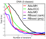
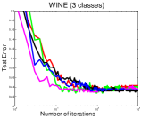
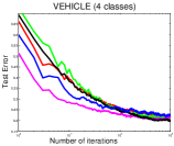
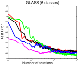
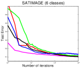
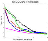
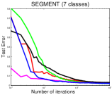
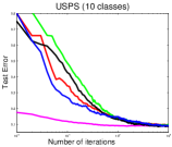
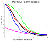
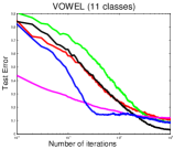
Figure 4: Average test error curves on multi-class UCI data sets. The vertical axis denotes the averaged test error rate and the horizontal axis denotes the number of boosting iterations. Best viewed in color.

The next experiment is conducted on both binary and multi-class UCI machine learning repository and Statlog data sets. For binary classification problems, we compare our approaches with AdaBoost [24] while for multi-class problems, we compare our approaches with AdaBoost.MH [26], AdaBoost.MO [26], AdaBoost.ECC [7] and MultiBoost [27]. Each data set is then randomly split into two groups: $75\%$ of samples for training and the rest for evaluation. We set the maximum number of boosting iterations to $1000$. For AdaBoost.MH, AdaBoost.MO and AdaBoost.ECC, the training stops when the algorithm converges, e.g., when the weighted error of weak classifiers is greater than $0.5$. For MultiBoost, we use the logistic loss and choose the regularization parameter from $\{10^{-8},10^{-7},10^{-6},10^{-5},10^{-4}\}$. For RBoost${}^{\,\text{rank}}$, we set $n$ to be $2\cdot 10^{4}$. For RBoost${}^{\,\text{proj}}$, we set $n$ to be equal to the number of boosting iterations, i.e., $1000$. Note that we have not carefully tuned $n$ in this experiment. The regularization parameter, $\nu$, is determined by $5$-fold cross validation. We choose the best $\nu$ from $\{10^{-5},10^{-4},10^{-3},10^{-2}\}$ for binary problems and from $\{10^{-8},$ $2.5\times 10^{-8},$ $5\times 10^{-8},$ $7.5\times 10^{-8},$ $10^{-7},\cdots,10^{-2}\}$ for multi-class problems. The training stops when adding more weak classifiers does not further decrease the objective function of (18). All experiments are repeated $10$ times and the mean and standard deviation of test errors are reported in Tables IV and V. For binary classification problems, we observe that all methods perform similarly. This indicates that random projection based classifiers work well in practice. This is not surprising since it can be shown easily that, for two-class problems, RBoost${}^{\,\text{rank}}$ simply performs AdaBoost on the randomly projected data [17]. By the theory of random projections one would expect the performance of AdaBoost trained using the data in the original space to be similar to that of AdaBoost trained using the randomly projected data. For multi-class problems, we observe that most methods perform very similarly. However, RBoost${}^{\,\text{rank}}$ has a slightly better generalization performance than other multi-class boosting algorithms on $5$ out of $11$ data sets while RBoost${}^{\,\text{proj}}$ performs slightly better than other algorithms on $3$ out of $11$ data sets.

We then statistically compare both proposed approaches using the nonparametric Wilcoxon signed-rank test (WSRT) [31]. WSRT tests the median performance difference between RBoost${}^{\,\text{proj}}$ and RBoost${}^{\,\text{rank}}$. In this test, we set the significance level to be $5\%$. The null-hypothesis declares that there is no difference between the median performance of both algorithms at the $5\%$ significance level, i.e., both algorithms perform equally well in a statistical sense. According to the table of exact critical values for the Wilcoxon’s test, for a confidence level of $0.05$ and $11$ data sets, the difference between the classifiers is significant if the smaller of the rank sums is equal or less than $10$. Since the signed rank statistic result ($16$) is not less than the critical value ($10$), WSRT indicates a failure to reject the null hypothesis at the $5\%$ significance level. In other words, the test statistics suggest that both RBoost${}^{\,\text{proj}}$ and RBoost${}^{\,\text{rank}}$ perform equally well.

We further conduct an additional experiment on RBoost${}^{\,\text{rank}}$ and RBoost${}^{\,\text{proj}}$ using a different weak classifier. An alternative choice of weak classifiers for training boosting classifiers is weighted Fisher linear discriminant analysis (WLDA) [32]. WLDA learns a linear projection function which ensures good class separation between normally distributed samples of two classes. The linear projection function is defined as $(\Sigma_{1}+\Sigma_{2})^{-1}(\mu_{1}-\mu_{2})$ where $\mu_{1}$ and $\mu_{2}$ are weighted class mean, and $\Sigma_{1}$ and $\Sigma_{2}$ are weighted class covariance matrices of the first and second class, respectively. In our experiment, we project the weighted input data to a line using WLDA and train the decision stump on the new $1$D data [32]. Although WLDA has a closed-form solution, computing the inverse of the covariance matrix can be computationally expensive when the size of covariance matrices is large, i.e., the time complexity is cubic in the size of covariance matrices which is $O([\min(n,(m-1)k)]^{3})$. For RBoost${}^{\,\text{rank}}$, it is computationally infeasible to find the inverse of the covariance matrices when $n$ ($n=20,000$) and $(m-1)k$ is large. The is one of the advantages for RBoost${}^{\,\text{rank}}$, compared with RBoost${}^{\,\text{proj}}$.

So instead we randomly select $1000$ dimensions from $n$ at each boosting iteration and then apply WLDA. We concatenate the new WLDA feature to $n$ randomly projected features and train RBoost${}^{\,\text{rank}}$. The average classification error of both approaches is shown in Table VI. 1) We observe that the performance of both approaches often improves when we apply a more discriminative WLDA as the weak learner, compared with decision stumps. 2) Again, we statistically compare the performance of both proposed approaches (with WLDA as the weak learner). Since the signed rank statistic result ($10.5$) is not less than the critical value ($0$), WSRT indicates a failure to reject the null hypothesis at the $5\%$ significance level. In summary, both algorithms also perform equally well when WLDA is used as the weak learner. Note that other weak learners, e.g., LIBLINEAR and radial basis function (RBF), may also be applied here.

We plot average test error curves of multi-class UCI data sets in Fig. 4. Again, we can see that both of the proposed methods perform similarly.

Data set	RBoost${}^{\,\text{rank}}$ (WLDA)	RBoost${}^{\,\text{proj}}$ (WLDA)
svmguide2 ($3$ classes)	$\mathbf{18.9}$ ($\mathbf{3.1}$)	$19.7$ ($2.6$)
wine ($3$ classes)	$3.2$ ($2.9$)	$\mathbf{2.5}$ ($\mathbf{3.1}$)
vehicle ($4$ classes)	$19.6$ ($2.3$)	$\mathbf{18.4}$ ($\mathbf{2.6}$)
glass ($6$ classes)	$25.9$ ($4.0$)	$\mathbf{22.5}$ ($\mathbf{4.2}$)
pendigits ($10$ classes)	$\mathbf{2.8}$ ($\mathbf{0.9}$)	$4.0$ ($1.2$)
vowel ($11$ classes)	$\mathbf{2.6}$ ($\mathbf{1.1}$)	$4.5$ ($1.8$)

TABLE VI: Average test errors (shown in $\%$) with linear perceptron classifiers trained by weighted linear discriminant analysis (WLDA) as the weak learner.

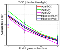
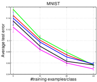
Figure 5: Average test errors on handwritten digits data sets by varying the amount of training samples per class. left: TiCC. right: MNIST. Best viewed in color.

IV-D Handwritten digits data sets

In this experiment, we vary the number of training samples and compare the performance of different boosting algorithms. We evaluate our algorithms on popular handwritten digits data sets (MNIST) and a more difficult handwritten character data sets (TiCC) [33]. We first resize the original image to a resolution of $28\times 28$ pixels and apply a deslant technique, similar to the one applied in [34]. We then extract $3$ levels of HOG features with $50\%$ block overlapping (spatial pyramid scheme) [35]. The block size in each level is $4\times 4$, $7\times 7$ and $14\times 14$ pixels, respectively. Extracted HOG features from all levels are concatenated. In total, there are $2,172$ HOG features. We perform dimensionality reduction using Principal Component Analysis (PCA) on training samples (similar to PCA-SIFT [36]). Our PCA projected data captures $90\%$ of the original data variance. For RBoost${}^{\,\text{rank}}$, we set $n$ to be $100K$. For RBoost${}^{\,\text{proj}}$, we choose the best parameter from $\{5\times 10^{-8},10^{-7},5\times 10^{-7},10^{-6},5\times 10^{-6},10^{-5}\}$. For MNIST, we randomly select $5$, $10$, $20$ and $40$ samples as training sets and use the original test sets of $10,000$ samples. For TiCC, we randomly select $5$, $10$, $20$ and $40$ samples from each class as training sets and use $50$ unseen samples from each class as test sets. All experiments are repeated $5$ times ($1000$ boosting iterations) and the results are summarized in Fig. 5. For handwritten digits, we observe that our algorithms and AdaBoost.MO perform slightly better than AdaBoost.ECC and AdaBoost.MH.

Note that AdaBoost.MO trains $2^{k-1}-1$ weak classifiers at each iteration, while both of our algorithms train $1$ weak classifier at each iteration. For example, on MNIST digit data sets, the AdaBoost.MO model would have a total of $511,000$ weak classifiers ($1000$ boosting iteration) while our multi-class classifier would only consist of $1000$ weak classifiers. In other words, AdaBoost.MO is $511$ times slower during performance evaluation. We suspect that these additional weak classifiers improve the generalization performance of AdaBoost.MO for handwritten digits data sets, where there is a large variation within the same class label.

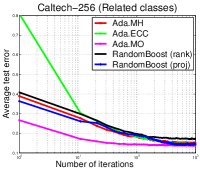
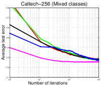
Figure 6: Average test error curves on Caltech-$256$ data sets. left: Related classes. right: Mixed classes. Best viewed in color.

IV-E Caltech-$256$ data sets

We also evaluate our algorithms on a subset of Caltech-$256$. We consider two types of classes as experimented in [37]: related classes and mixed classes. We use the same pre-computed features used in [38], i.e., PHOG, appearance, region covariance and LBP. The data set is randomly split into two groups: $25\%$ for training and the rest for evaluation. On average, there are $56$ training samples per class for related classes and $48$ training samples per class for mixed classes. We use the same setting as in the handwritten digits experiment. The average test accuracies of $5$ runs are reported in Fig. 6. We see again that AdaBoost.MO converges faster. This is not surprising as we previously mentioned that AdaBoost.MO trains $2^{k-1}-1$ weak classifiers at each iteration. As AdaBoost.MO is not scalable on a large number of classes, it is extremely slow during performance evaluation. Based on our experiments, AdaBoost.MO requires approximately $2^{k-1}$ times as much execution time as other algorithms during test time. The second observation is that our proposed methods usually converge slightly faster than AdaBoost.MH and AdaBoost.MH.

V Conclusion

We have shown that, by exploiting random projections, it is possible to devise a single-vector parameterized boosting-based classifier, which is capable of performing multi-class classification. This approach represents a significant divergence from existing multi-class classification approaches, as neither the number of classifiers, nor the number of parameters will grow as the number of classes increases. We have demonstrated two examples of the proposed approach, in the form of multi-class boosting algorithms, which solve the pairwise ranking problem and pairwise loss in the large margin framework. These algorithms are effective and can cope with both binary and multi-class classification problems as demonstrated on both synthetic and real world data sets.

Our goal thus far has been to formulate a single-vector multi-class boosting classifier, which demonstrates promising results and alleviate the proliferation of parameters typically faced in large-scale problems. Reducing the training time required by both methods for large-scale problems is yet another challenging issue. Techniques, such as approximating the weak classifiers’ threshold [39], approximating the weak classifiers using FilterBoost [40] or incremental weak classifier learning [41], offer an interesting approach towards this goal. An exploration on the effect of the size of random projection matrices on convergence and scaling could also be carried out.

Appendix A Proof of Theorem 1

Margin Preservation

If the boosting has margin $\gamma$, then for any $\delta,\epsilon\in(0,1)$ and any

$$n>\frac{12}{3\epsilon^{2}-2\epsilon^{3}}\ln\frac{6km}{\delta},$$

with probability at least $1-\delta$, the boosting associated with projected weak learners’ coefficients, ${\mathbf{P}}{\boldsymbol{w}}_{r},\forall r$, and the projected weak learners’ response, ${\mathbf{P}}{\mathbf{H}}$, has margin no less than

$$-\frac{1+3\epsilon}{1-\epsilon^{2}}+\frac{\sqrt{1-\epsilon^{2}}}{1+\epsilon}+\frac{1+\epsilon}{1-\epsilon}\gamma.$$

Proof:

By margin definition, for all $({\boldsymbol{x}},y)\in S$

$$\frac{\left\langle{\boldsymbol{w}}_{y},{\bf H}({\boldsymbol{x}})\right\rangle}{{\|{\boldsymbol{w}}_{y}\|}{\|{\bf H}({\boldsymbol{x}})\|}}-\max_{y^{\prime}\neq y}\frac{\left\langle{\boldsymbol{w}}_{y^{\prime}},{\bf H}({\boldsymbol{x}})\right\rangle}{{\|{\boldsymbol{w}}_{y^{\prime}}\|}{\|{\bf H}({\boldsymbol{x}})\|}}\geq\gamma.$$

Take any single $({\boldsymbol{x}},y)\in S$, and let $\hat{y}=\mathop{\mathrm{argmax}}\limits_{y^{\prime}}\frac{\left\langle{\boldsymbol{w}}_{y^{\prime}},{\bf H}({\boldsymbol{x}})\right\rangle}{{\|{\boldsymbol{w}}_{y^{\prime}}\|}{\|{\bf H}({\boldsymbol{x}})\|}}$ and $\hat{\hat{y}}=\mathop{\mathrm{argmax}}\limits_{y^{\prime\prime}}\frac{\left\langle{\bf P}{\boldsymbol{w}}_{y^{\prime\prime}},{\bf P}{\bf H}({\boldsymbol{x}})\right\rangle}{{\|{\bf P}{\boldsymbol{w}}_{y^{\prime\prime}}\|}{\|{\bf P}{\bf H}({\boldsymbol{x}})\|}}$, we have by Lemma 1 (substituting ${\boldsymbol{x}}$ in Lemma 1 by ${\bf H}({\boldsymbol{x}})$ ) and union bound over all $y^{\prime}\neq y$

$$\Pr\Big{(}\frac{\left\langle{\bf P}{\boldsymbol{w}}_{y},{\bf P}{\bf H}({\boldsymbol{x}})\right\rangle}{\|{{\bf P}{\boldsymbol{w}}_{y}}\|\|{{\bf P}{\bf H}({\boldsymbol{x}})}\|} \geq 1-\frac{1+\epsilon}{1-\epsilon}\big{(}1-\frac{\left\langle{\boldsymbol{w}}_{y},{\bf H}({\boldsymbol{x}})\right\rangle}{\|{{\boldsymbol{w}}_{y}}\|\|{{\bf H}({\boldsymbol{x}})}\|}\big{)}\Big{)}$$

$$\geq 1-6\exp{(-\frac{n}{2}(\frac{\epsilon^{2}}{2}-\frac{\epsilon^{3}}{3}))},$$

$$\Pr\Big{(}\forall y^{\prime}\neq y,$$

$$\frac{\left\langle{\bf P}{\boldsymbol{w}}_{y^{\prime}},{\bf P}{\bf H}({\boldsymbol{x}})\right\rangle}{\|{{\bf P}{\boldsymbol{w}}_{y^{\prime}}}\|\|{{\bf P}{\bf H}({\boldsymbol{x}})}\|} \leq 1-\frac{\sqrt{1-\epsilon^{2}}}{1+\epsilon}+\frac{\epsilon}{1+\epsilon}$$

$$+\frac{1-\epsilon}{1+\epsilon}\cdot\frac{\left\langle{\boldsymbol{w}}_{y^{\prime}},{\bf H}({\boldsymbol{x}})\right\rangle}{\|{{\boldsymbol{w}}_{y^{\prime}}}\|\|{{\bf H}({\boldsymbol{x}})}\|}\Big{)}$$

$$\geq 1-6(k-1)\exp{\left(-\frac{n}{2}\cdot(\frac{\epsilon^{2}}{2}-\frac{\epsilon^{3}}{3})\right)}.$$

By the union bound again, with probability at least

$$1-6km\cdot\exp{\left(-\frac{n}{2}(\frac{\epsilon^{2}}{2}-\frac{\epsilon^{3}}{3})\right)}$$

for all $({\boldsymbol{x}},y)\in S$, we have

$$\frac{\left\langle{\bf P}{\boldsymbol{w}}_{y},{\bf P}{\bf H}({\boldsymbol{x}})\right\rangle}{\|{{\bf P}{\boldsymbol{w}}_{y}}\|\|{{\bf P}{\bf H}({\boldsymbol{x}})}\|}-\max_{y^{\prime}\neq y}\frac{\left\langle{\bf P}{\boldsymbol{w}}_{y^{\prime}},{\bf P}{\bf H}({\boldsymbol{x}})\right\rangle}{\|{{\bf P}{\boldsymbol{w}}_{y^{\prime}}}\|\|{{\bf P}{\bf H}({\boldsymbol{x}})}\|}$$

$$\geq -\frac{1+3\epsilon}{1-\epsilon^{2}}+\frac{\sqrt{1-\epsilon^{2}}}{1+\epsilon}+\frac{1+\epsilon}{1-\epsilon}\gamma$$

Let $\delta=6km\exp{(-\frac{n}{2}(\frac{\epsilon^{2}}{2}-\frac{\epsilon^{3}}{3}))}$, we have the desirable lower bound on $n$. ∎

Appendix B Proof of Theorem 2

Single-vector Multi-class Boosting

Given any random Gaussian matrix ${\mathbf{R}}\in\mathbb{R}^{n\times kT}$, whose entry ${\mathbf{R}}(i,j)=$ $\frac{1}{\sqrt{n}}{a_{ij}}$ where $a_{ij}$ is i.i.d. random variables from $\operatorname{\mathcal{N}}(0,1)$. Denote ${\mathbf{P}}_{y}\in\mathbb{R}^{n,T}$ as the $y$-th submatrix of ${\mathbf{R}}$, that is ${\mathbf{R}}=[{\mathbf{P}}_{1},$ $\cdots,{\mathbf{P}}_{r},$ $\cdots,$ ${\mathbf{P}}_{k}]$. If the boosting has margin $\gamma$, then for any $\delta,\epsilon\in(0,1]$ and any

$$n>\frac{12}{3\epsilon^{2}-2\epsilon^{3}}\ln{\frac{6m(k-1)}{\delta}},$$

there exists a single-vector ${\boldsymbol{v}}\in\mathbb{R}^{n}$, such that

$$\Pr\Big{(} \frac{\left\langle{\boldsymbol{v}},{\mathbf{P}}_{y}{\mathbf{H}}({\boldsymbol{x}})\right\rangle-\left\langle{\boldsymbol{v}},{\mathbf{P}}_{y^{\prime}}{\mathbf{H}}({\boldsymbol{x}})\right\rangle}{\|{\boldsymbol{v}}\|\sqrt{\|{\mathbf{P}}_{y}{\mathbf{H}}({\boldsymbol{x}})\|^{2}+\|{\mathbf{P}}_{y^{\prime}}{\mathbf{H}}({\boldsymbol{x}})\|^{2}}}\geq$$

$$\frac{-2\epsilon}{1-\epsilon}+\frac{1+\epsilon}{{\sqrt{2k}}(1-\epsilon)}\gamma\Big{)}\geq 1-\delta,\quad\quad\forall y^{\prime}\neq y.$$ (27)

Proof:

By the margin definition, there exists ${\boldsymbol{w}}$, such that for all $({\bf H}({\boldsymbol{x}}),y)\in S$,

$$\frac{\left\langle{\boldsymbol{w}}_{y},{\bf H}({\boldsymbol{x}})\right\rangle}{\|{{\boldsymbol{w}}_{y}}\|\|{{\bf H}({\boldsymbol{x}})}\|}-\frac{\left\langle{\boldsymbol{w}}_{y^{\prime}},{\bf H}({\boldsymbol{x}})\right\rangle}{\|{{\boldsymbol{w}}_{y^{\prime}}}\|\|{{\bf H}({\boldsymbol{x}})}\|}\geq\gamma,\forall y^{\prime}\neq y.$$

Without losing generality, we assume ${\boldsymbol{w}}_{y}$ has unit length, which can always be achieved by normalization, for all $y$. So now

$${\left\langle{\boldsymbol{w}}_{y},{\bf H}({\boldsymbol{x}})\right\rangle}-{\left\langle{\boldsymbol{w}}_{y^{\prime}},{\bf H}({\boldsymbol{x}})\right\rangle}\geq\gamma{\|{{\bf H}({\boldsymbol{x}})}\|},\forall y^{\prime}\neq y.$$

This can be rewritten as

$$\left\langle{\bf u},{\bf H}({\boldsymbol{x}})\otimes{\bf e}_{y}\right\rangle-\left\langle{\bf u},{\bf H}({\boldsymbol{x}})\otimes{{\bf e}_{y^{\prime}}}\right\rangle=$$

$$\left\langle{\bf H}({\boldsymbol{x}})\otimes{\bf e}_{y}-{\bf H}({\boldsymbol{x}})\otimes{\bf e}_{y^{\prime}},{\bf u}\right\rangle\geq\gamma{\|{{\bf H}({\boldsymbol{x}})}\|},$$

where ${\bf u}$ is the concatenation of all ${\boldsymbol{w}}_{y}$, i.e. ${\bf u}=[{\boldsymbol{w}}_{1}^{\!\top},\cdots,{\boldsymbol{w}}_{y}^{\!\top},\cdots{\boldsymbol{w}}_{k}^{\!\top}]^{\!\top}$; the vector ${\bf e}_{y}\in\mathbb{R}^{k}$ with 1 at the $y$-th dimension and zeros in others, and $\otimes$ is the tensor product. Define ${\boldsymbol{z}}_{{\boldsymbol{x}},y^{\prime}}={\bf H}({\boldsymbol{x}})\otimes{\bf e}_{y}-{\bf H}({\boldsymbol{x}})\otimes{\bf e}_{y^{\prime}}$.

Applying Lemma 1 to ${\bf u}$ and ${\boldsymbol{z}}_{{\boldsymbol{x}},y^{\prime}}$, we have for a given $({\boldsymbol{x}},y)$ and a fixed $y^{\prime}\neq y$, with probability at least $1-6\exp{(-\frac{n}{2}(\frac{\epsilon^{2}}{2}-\frac{\epsilon^{3}}{3}))}$, the following holds,

$$\frac{\left\langle{\bf P}{\bf u},{\bf P}{\boldsymbol{z}}_{{\boldsymbol{x}},y^{\prime}}\right\rangle}{\|{\bf P}{\bf u}\|\|{\bf P}{\boldsymbol{z}}_{{\boldsymbol{x}},y^{\prime}}\|}$$

$$\geq 1-\frac{1+\epsilon}{1-\epsilon}\left(1-\frac{\left\langle{\bf H}({\boldsymbol{x}})\otimes{\bf e}_{y}-{\bf H}({\boldsymbol{x}})\otimes{\bf e}_{y^{\prime}},{\bf u}\right\rangle}{\sqrt{2}\|{\bf u}\|\|{\bf H}({\boldsymbol{x}})\|}\right)$$

$$=1-\frac{1+\epsilon}{1-\epsilon}+$$

$$\frac{1+\epsilon}{{\sqrt{2}}(1-\epsilon)}\left(\frac{\left\langle{\boldsymbol{w}}_{y},{\bf H}({\boldsymbol{x}})\right\rangle}{\|{\bf u}\|\|{\bf H}({\boldsymbol{x}})\|}-\frac{\left\langle{\boldsymbol{w}}_{y^{\prime}},{\bf H}({\boldsymbol{x}})\right\rangle}{\|{\bf u}\|\|{\bf H}({\boldsymbol{x}})\|}\right)$$

$$\geq 1-\frac{1+\epsilon}{1-\epsilon}+\frac{1+\epsilon}{{\sqrt{2k}}(1-\epsilon)}\gamma$$

$$=\frac{-2\epsilon}{1-\epsilon}+\frac{1+\epsilon}{{\sqrt{2k}}(1-\epsilon)}\gamma.$$

By the union bound over $m$ samples and $k-1$ many $y^{\prime}$,

$$\Pr\Big{(} \exists({\boldsymbol{x}},y)\in S,\exists y^{\prime}\neq y,$$

$$\frac{\left\langle{\bf P}{\bf u},{\bf P}{\boldsymbol{z}}_{{\boldsymbol{x}},y^{\prime}}\right\rangle}{\|{\bf P}{\bf u}\|\|{\bf P}{\boldsymbol{z}}_{{\boldsymbol{x}},y^{\prime}}\|}<\frac{-2\epsilon}{1-\epsilon}+\frac{1+\epsilon}{{\sqrt{2L}}(1-\epsilon)}\gamma\Big{)}$$

$$\leq 6m(k-1)\exp{\left(-\frac{n}{2}\cdot(\frac{\epsilon^{2}}{2}-\frac{\epsilon^{3}}{3})\right)}.$$

Let ${\boldsymbol{q}}={\bf P}{\bf u}$, we have

$$\left\langle{\bf P}{\bf u},{\bf P}{\boldsymbol{z}}_{{\boldsymbol{x}},y^{\prime}}\right\rangle=\left\langle{\boldsymbol{q}},{\bf P}_{y}{\boldsymbol{x}}-{\bf P}_{y^{\prime}}{\boldsymbol{x}}\right\rangle.$$

Setting $\delta=6m(k-1)\exp{(-\frac{n}{2}(\frac{\epsilon^{2}}{2}-\frac{\epsilon^{3}}{3}))}$ gives the bound on $n$. Thus

$$\Pr\Big{(} \forall({\boldsymbol{x}},y)\in S,\forall y^{\prime}\neq y,$$

$$\frac{\left\langle{\boldsymbol{q}},{\bf P}_{y}{\bf H}({\boldsymbol{x}})\right\rangle-\left\langle{\boldsymbol{q}},{\bf P}_{y^{\prime}}{\bf H}({\boldsymbol{x}})\right\rangle}{\|{\boldsymbol{q}}\|\sqrt{\|{\bf P}_{y}{\bf H}({\boldsymbol{x}})\|^{2}+\|{\bf P}_{y^{\prime}}{\bf H}({\boldsymbol{x}})\|^{2}}}\geq$$

$$\frac{-2\epsilon}{1-\epsilon}+\frac{1+\epsilon}{{\sqrt{2k}}(1-\epsilon)}\gamma\Big{)}\geq 1-\delta,$$

which concludes the proof. ∎

We have used the following two lemmas for proving the above two theorems.

Lemma 1

For any ${\boldsymbol{w}},{\boldsymbol{x}}\in\mathbb{R}^{d}$, any random Gaussian matrix ${\bf P}\in\mathbb{R}^{n,d}$ whose entry ${\bf P}(i,j)=\frac{1}{\sqrt{n}}{a_{ij}}$ where $a_{ij}$s are i.i.d. random variables from $\operatorname{\mathcal{N}}(0,1)$,

$$\gamma=\frac{\left\langle{\boldsymbol{w}},{\boldsymbol{x}}\right\rangle}{\|{\boldsymbol{w}}\|\|{\boldsymbol{x}}\|},$$

for any $\epsilon\in(0,1)$, if $\gamma\in(0,1]$, then with probability at least

$$1-6\exp{(-\frac{n}{2}(\frac{\epsilon^{2}}{2}-\frac{\epsilon^{3}}{3}))},$$

the following holds

$$1-\frac{(1+\epsilon)}{(1-\epsilon)}{(1-\gamma)}\leq\frac{\left\langle{\bf P}{\boldsymbol{w}},{\bf P}{\boldsymbol{x}}\right\rangle}{\|{{\bf P}{\boldsymbol{w}}}\|\|{{\bf P}{\boldsymbol{x}}}\|}$$

$$\leq 1-\frac{\sqrt{(1-\epsilon^{2})}}{(1+\epsilon)}+\frac{\epsilon}{(1+\epsilon)}+\frac{(1-\epsilon)}{(1+\epsilon)}{\gamma}.$$ (28)

Proof:

From Lemma 2 and union bound, we know

$$(1-\epsilon)\leq\frac{\|{{\bf P}{\boldsymbol{x}}}\|^{2}}{\|{\boldsymbol{x}}\|^{2}}\leq(1+\epsilon),(1-\epsilon)\leq\frac{\|{{\bf P}{\boldsymbol{w}}}\|^{2}}{\|{\boldsymbol{w}}\|^{2}}\leq(1+\epsilon)$$ (29)

holds with probability at least $1-4\exp{(-\frac{n}{2}(\frac{\epsilon^{2}}{2}-\frac{\epsilon^{3}}{3}))}$. When (29) holds, due to the fact that increasing the length of two unit length vectors (i.e. from $\frac{{\bf P}{\boldsymbol{x}}}{\|{\bf P}{\boldsymbol{x}}\|}$ and $\frac{{\bf P}{\boldsymbol{w}}}{\|{\bf P}{\boldsymbol{w}}\|}$ to $\frac{{\bf P}{\boldsymbol{x}}}{\sqrt{(1-\epsilon)}\|{\boldsymbol{x}}\|}$ and $\frac{{\bf P}{\boldsymbol{w}}}{\sqrt{(1-\epsilon)}\|{\boldsymbol{w}}\|}$) increases the norm of their difference, we have

$$\left\|\frac{{\bf P}{\boldsymbol{x}}}{\|{\bf P}{\boldsymbol{x}}\|}-\frac{{\bf P}{\boldsymbol{w}}}{\|{\bf P}{\boldsymbol{w}}\|}\right\|^{2}\leq\left\|\frac{{\bf P}{\boldsymbol{x}}}{\sqrt{(1-\epsilon)}\|{\boldsymbol{x}}\|}-\frac{{\bf P}{\boldsymbol{w}}}{\sqrt{(1-\epsilon)}\|{\boldsymbol{w}}\|}\right\|^{2}.$$ (30)

It is easy to prove that

$$\left\|\frac{{\bf P}{\boldsymbol{x}}}{\|{\boldsymbol{x}}\|}-\frac{{\bf P}{\boldsymbol{w}}}{\|{\boldsymbol{w}}\|}\right\|^{2}\leq \left\|\sqrt{(1-\epsilon)}\frac{{\bf P}{\boldsymbol{x}}}{\|{\bf P}{\boldsymbol{x}}\|}-\sqrt{(1+\epsilon)}\frac{{\bf P}{\boldsymbol{w}}}{\|{\bf P}{\boldsymbol{w}}\|}\right\|^{2}$$

$$\leq \left\|\sqrt{(1+\epsilon)}(\frac{{\bf P}{\boldsymbol{x}}}{\|{\bf P}{\boldsymbol{x}}\|}-\frac{{\bf P}{\boldsymbol{w}}}{\|{\bf P}{\boldsymbol{w}}\|})\right\|^{2}$$

$$+(\sqrt{(1+\epsilon)}-\sqrt{(1-\epsilon)})^{2}.$$ (31)

The first inequality is due to (29), the second inequality is due to the property of an acute angle.

Applying Lemma 2 to the vector $\left(\frac{{\boldsymbol{x}}}{\|{\boldsymbol{x}}\|}-\frac{{\boldsymbol{w}}}{\|{\boldsymbol{w}}\|}\right)$, we have

$${(1-\epsilon)}\left\|\frac{{\boldsymbol{x}}}{\|{\boldsymbol{x}}\|}-\frac{{\boldsymbol{w}}}{\|{\boldsymbol{w}}\|}\right\|^{2}\leq\left\|\frac{{\bf P}{\boldsymbol{x}}}{\|{\boldsymbol{x}}\|}-\frac{{\bf P}{\boldsymbol{w}}}{\|{\boldsymbol{w}}\|}\right\|^{2}$$

$$\leq{(1+\epsilon)}\left\|\frac{{\boldsymbol{x}}}{\|{\boldsymbol{x}}\|}-\frac{{\boldsymbol{w}}}{\|{\boldsymbol{w}}\|}\right\|^{2}$$ (32)

holds for certain probability.

Let $\beta$ be the angle of ${\boldsymbol{w}}$ and ${\boldsymbol{x}}$, and $\alpha$ be the angle of ${\bf P}{\boldsymbol{w}}$ and ${\bf P}{\boldsymbol{x}}$, we have

$$\gamma=\frac{\left\langle{\boldsymbol{w}},{\boldsymbol{x}}\right\rangle}{\|{{\boldsymbol{w}}}\|\|{{\boldsymbol{x}}}\|}=\cos(\beta)=1-2\sin^{2}(\frac{\beta}{2})$$

$$=1-\frac{1}{2}\left\|\frac{{\boldsymbol{x}}}{\|{\boldsymbol{x}}\|}-\frac{{\boldsymbol{w}}}{\|{\boldsymbol{w}}\|}\right\|^{2}.$$ (33)

Similarly

$$\frac{\left\langle{\bf P}{\boldsymbol{w}},{\bf P}{\boldsymbol{x}}\right\rangle}{\|{{\bf P}{\boldsymbol{w}}}\|\|{{\bf P}{\boldsymbol{x}}}\|}=1-\frac{1}{2}\left\|\frac{{\bf P}{\boldsymbol{x}}}{\|{\bf P}{\boldsymbol{x}}\|}-\frac{{\bf P}{\boldsymbol{w}}}{\|{\bf P}{\boldsymbol{w}}\|}\right\|^{2}.$$ (34)

Using (32), (30) and (31) we get $\left\|\frac{{\bf P}{\boldsymbol{x}}}{\|{\bf P}{\boldsymbol{x}}\|}-\frac{{\bf P}{\boldsymbol{w}}}{\|{\bf P}{\boldsymbol{w}}\|}\right\|^{2}$ is bounded below and above by two terms involving $\left\|\frac{{\boldsymbol{x}}}{\|{\boldsymbol{x}}\|}-\frac{{\boldsymbol{w}}}{\|{\boldsymbol{w}}\|}\right\|^{2}$. Plugging (33) and (34) into the two side bounds, we get (28). Here we applied Lemma 2 to 3 vectors, namely ${\boldsymbol{x}}$, ${\boldsymbol{w}}$, and $(\frac{{\boldsymbol{x}}}{\|{\boldsymbol{x}}\|}-\frac{{\boldsymbol{w}}}{\|{\boldsymbol{w}}\|})$, thus by union bound, the probability of the above holds is at least $1-6\exp{(-\frac{n}{2}(\frac{\epsilon^{2}}{2}-\frac{\epsilon^{3}}{3}))}$. ∎

Lemma 2

For any ${\boldsymbol{x}}\in\mathbb{R}^{T}$, any random Gaussian matrix ${\bf P}\in\mathbb{R}^{n\times T}$ whose entry ${\bf P}(i,j)=\frac{1}{\sqrt{n}}{a_{ij}}$ where $a_{ij}$s are i.i.d. random variables from $\operatorname{\mathcal{N}}(0,1)$, for any $\epsilon\in(0,1)$,

$$\Pr\Big{(}(1-\epsilon)\leq\frac{\|{{\bf P}{\boldsymbol{x}}}\|^{2}}{\|{\boldsymbol{x}}\|^{2}}\leq(1+\epsilon)\Big{)}$$

$$\geq 1-2\exp{(-\frac{n}{2}(\frac{\epsilon^{2}}{2}-\frac{\epsilon^{3}}{3}))}.$$

Proof:

Obviously, for any ${\boldsymbol{w}},{\boldsymbol{x}}\in\mathbb{R}^{T}$, the following holds:

$${\mathbb{E}}(\left\langle{\bf P}{\boldsymbol{w}},{\bf P}{\boldsymbol{x}}\right\rangle)$$

$$= \frac{1}{n}{\mathbb{E}}\Big{[}\sum_{\ell=1}^{n}\Big{(}\sum_{j=1}^{d}a_{\ell j}w_{j}\sum_{i=1}^{d}a_{\ell i}x_{i}\Big{)}\Big{]}$$

$$= \frac{1}{n}\sum_{\ell=1}^{n}\Big{(}\sum_{j=1}^{d}{\mathbb{E}}(a_{\ell j}^{2})w_{j}x_{j}$$

$$+\sum_{j=1}^{d}{\mathbb{E}}(a_{\ell j})w_{j}\sum_{i\neq j:i=1}^{d}{\mathbb{E}}(a_{\ell i})x_{i}\Big{)}.$$

$$= \left\langle{\boldsymbol{w}},{\boldsymbol{x}}\right\rangle.$$

To obtain above, we only used the fact that $\{a_{ij}\}$ are independent with zero mean and unit variance.

Due to 2-stability of Gaussian distribution, we know $\sum_{j=1}^{d}a_{\ell j}w_{j}=\|{\boldsymbol{w}}\|z_{\ell}$ and $\sum_{j=1}^{d}a_{\ell j}x_{j}=\|{\boldsymbol{x}}\|z^{\prime}_{\ell}$, where ${z_{\ell}}$ and ${z^{\prime}_{\ell}}\sim\operatorname{\mathcal{N}}(0,1)$. we have $\left\langle{\bf P}{\boldsymbol{w}},{\bf P}{\boldsymbol{x}}\right\rangle=\frac{1}{n}\|{\boldsymbol{w}}\|\|{\boldsymbol{x}}\|\sum_{\ell=1}^{n}z_{\ell}z^{\prime}_{\ell}$. If ${\boldsymbol{w}}={\boldsymbol{x}}$, $\sum_{\ell=1}^{n}z^{2}_{\ell}$ is chi-square distributed with $n$-degree freedom. Applying the standard tail bound of chi-square distribution, we have

$$\Pr\Big{(}\left\langle{\bf P}{\boldsymbol{w}},{\bf P}{\boldsymbol{x}}\right\rangle\leq(1-\epsilon)\left\langle{\boldsymbol{w}},{\boldsymbol{x}}\right\rangle\Big{)}$$

$$\leq\exp{\Big{(}\frac{n}{2}(1-(1-\epsilon)+\ln(1-\epsilon))\Big{)}}\leq\exp{(-\frac{n}{4}\epsilon^{2})}.$$

Here we used the inequality $\ln(1-\epsilon)\leq-\epsilon-\epsilon^{2}/2$. Similarly, we have

$$\Pr\Big{(}\left\langle{\bf P}{\boldsymbol{w}},{\bf P}{\boldsymbol{x}}\right\rangle\leq(1+\epsilon)\left\langle{\boldsymbol{w}},{\boldsymbol{x}}\right\rangle\Big{)}$$

$$\leq\exp{\Big{(}\frac{n}{2}(1-(1+\epsilon)+\ln(1+\epsilon))\Big{)}}\leq\exp{(-\frac{n}{2}(\frac{\epsilon^{2}}{2}-\frac{\epsilon^{3}}{3}))}.$$

Here we used the inequality $\ln(1+\epsilon)\leq\epsilon-\epsilon^{2}/2+\epsilon^{3}/3$. ∎

References

- [1] N. Garcia-Pedrajas, “Constructing ensembles of classifiers by means of weighted instance selection,” IEEE Trans. Neural Networks, vol. 20, no. 2, pp. 258–277, 2009.
- [2] P. Sun and X. Yao, “Sparse approximation through boosting for learning large scale kernel machines,” IEEE Trans. Neural Networks, vol. 21, no. 6, pp. 883–894, 2010.
- [3] P. Wang, C. Shen, N. Barnes, and H. Zheng, “Fast and robust object detection using asymmetric totally corrective boosting,” IEEE Trans. Neural Networks & Learn. Systems, vol. 23, no. 1, pp. 33–46, 2012.
- [4] C. Shen and H. Li, “Boosting through optimization of margin distributions,” IEEE Trans. Neural Networks, vol. 21, no. 4, pp. 659–666, 2010.
- [5] E. L. Allwein, R. E. Schapire, and Y. Singer, “Reducing multiclass to binary: A unifying approach for margin classifiers,” J. Mach. Learn. Res., vol. 1, pp. 113–141, 2001.
- [6] T. Dietterich and G. Bakiri, “Solving multiclass learning problems via error-correcting output codes,” J. Artificial Intell. Res., vol. 2, pp. 263–286, 1995.
- [7] V. Guruswami and A. Sahai, “Multiclass learning, boosting, and error correcting codes,” in Proc. Annual Conf. Learn. Theory, 1999, pp. 145–155.
- [8] R. E. Schapire, “Using output codes to boost multiclass learning problems,” in Proc. Int. Conf. Mach. Learn., 1997.
- [9] C. Shen and H. Li, “On the dual formulation of boosting algorithms,” IEEE Trans. Pattern Anal. Mach. Intell., 2010.
- [10] E. J. Candes and T. Tao, “Near-optimal signal recovery from random projections: Universal encoding strategies?,” IEEE Trans. Info. Theory, vol. 52, no. 12, pp. 5406 –5425, 2006.
- [11] R. I. Arriaga and S. Vempala, “An algorithmic theory of learning: Robust concepts and random projection,” J. Mach. Learn. Res., vol. 63, no. 2, pp. 161–182, 2006.
- [12] X. Z. Fern and C. E. Broadley, “Random projection for high dimensional data clustering: A cluster ensemble approach,” in Proc. Int. Conf. Mach. Learn., 2003.
- [13] D. Fradkin and D. Madigan, “Experiments with random projections for machine learning,” in Proc. ACM Int. Conf. Knowledge discovery data mining, 2003.
- [14] P. Indyk and R. Motwani, “Approximate nearest neighbors: Towards removing the curse of dimensionality,” in Proc. Symp. Theory Comp., 1998.
- [15] Q. Shi, H. Li, and C. Shen, “Rapid face recognition using hashing,” in Proc. IEEE Conf. Comp. Vis. Patt. Recogn., 2010.
- [16] Y. Freund, R. Iyer, R. E. Schapire, and Y. Singer, “An efficient boosting algorithm for combining preferences,” J. Mach. Learn. Res., vol. 4, pp. 933–969, 2003.
- [17] C. Rudin and R. E. Schapire, “Margin-based ranking and an equivalence between AdaBoost and RankBoost,” J. Mach. Learn. Res., vol. 10, pp. 2193–2232, 2009.
- [18] A. Demiriz, K. P. Bennett, and J. Shawe-Taylor, “Linear programming boosting via column generation,” Mach. Learn., vol. 46, pp. 225–254, 2002.
- [19] A. Gionis, P. Indyk, and R. Motwani, “Similarity search in high dimensions via hashing,” in Proc. of Int. Conf. on Very Large Data Bases, 1999.
- [20] R. Cai, C. Zhang, L. Zhang, and W. Y. Ma, “Scalable music recommendation by search,” in Proc. Int. Conf. Multimedia, 2007.
- [21] Y. Ke, R. Sukthankar, and L. Huston, “Efficient near-duplicate detection and sub-image retrieval,” in Proc. Int. Conf. Multimedia, 2004.
- [22] E. Bingham and H. Mannila, “Random projection in dimensionality reduction: applications to image and text data,” in Proc. of ACM SIGKDD Int. Conf. Knowledge Discovery and Data Mining, 2001.
- [23] G. Shakhnarovich, P. Viola, and T. Darrell, “Fast pose estimation with parameter-sensitive hashing,” in Proc. IEEE Int. Conf. Comp. Vis., 2003.
- [24] Y. Freund and R. E. Schapire, “A decision-theoretic generalization of on-line learning and an application to boosting,” J. Comp. Sys. Sci., vol. 55, no. 1, pp. 119–139, 1997.
- [25] R. Rifkin and A. Klautau, “In defense of one-vs-all classification,” J. Mach. Learn. Res., vol. 5, pp. 101–141, 2004.
- [26] R. Schapire and Y. Singer, “Improved boosting algorithms using confidence-rated prediction,” Mach. Learn., vol. 37, no. 3, pp. 297 336, 1999.
- [27] C. Shen and Z. Hao, “A direct formulation for totally-corrective multi-class boosting,” in Proc. IEEE Conf. Comp. Vis. Patt. Recogn., 2011.
- [28] J. Friedman, T. Hastie, and R. Tibshirani, “Additive logistic regression: a statistical view of boosting,” Ann. Statist., vol. 28, no. 2, pp. 337–407, 2000.
- [29] Llew Mason, Jonathan Baxter, Peter L. Bartlett, and Marcus R. Frean, “Boosting algorithms as gradient descent.,” in Proc. Adv. Neural Inf. Process. Syst., 1999, pp. 512–518.
- [30] L. Li, “Multiclass boosting with repartitioning,” in Proc. Int. Conf. Mach. Learn., 2006, pp. 569–576.
- [31] J. Demvsar, “Statistical comparisons of classifiers over multiple data sets,” J. Mach. Learn. Res., vol. 7, pp. 1–30, 2006.
- [32] C. Shen, S. Paisitkriangkrai, and J. Zhang, “Face detection from few training examples,” in Proc. IEEE Int. Conf. Image Process., 2008.
- [33] L. van der Maaten, “A new benchmark data set for handwritten character recognition,” Technical Report, Tilburg University, 2009.
- [34] U. Meier, D. Ciresan, L. M. Gambardella, and J. Schmidhuber, “Better digit recognition with a committee of simple neural nets,” in Proc. Int. Conf. Doc. Anal. Recogn., 2011.
- [35] S. Lazebnik, C. Schmid, and J. Ponce, “Beyond bags of features: Spatial pyramid matching for recognizing natural scene categories,” in Proc. IEEE Conf. Comp. Vis. Patt. Recogn., 2006.
- [36] Y. Ke and R. Sukthankar, “Pca-sift: A more distinctive representation for local image descriptors,” in Proc. IEEE Conf. Comp. Vis. Patt. Recogn., 2004.
- [37] T. Tommasi, F. Orabona, and B. Caputo, “Safety in numbers: Learning categories from few examples with multi model knowledge transfer,” in Proc. IEEE Conf. Comp. Vis. Patt. Recogn., 2010.
- [38] P. Gehler and S. Nowozin, “On feature combination for multiclass object classification,” in Proc. IEEE Int. Conf. Comp. Vis., 2009.
- [39] M.-T. Pham and T.-J. Cham, “Fast training and selection of haar features using statistics in boosting-based face detection,” in Proc. IEEE Int. Conf. Comp. Vis., 2007.
- [40] J. K. Bradley and R. E. Schapire, “Filterboost: Regression and classification on large datasets,” in Proc. Adv. Neural Inf. Process. Syst., 2008.
- [41] Y. Pang, J. Deng, and Y. Yuan, “Incremental threshold learning for classifier selection,” Neurocomputing, vol. 89, pp. 89–95, 2012.