A Boltzmann treatment for the vorton excess problem

Abstract

We derive and solve a Boltzmann equation governing the cosmological evolution of the number density of current carrying cosmic string loops, whose centrifugally supported equilibrium configurations are also referred to as vortons. The phase space is three-dimensional and consists of the time variable, the loop size, and a conserved quantum number. Our approach includes gravitational wave emission, a possibly finite lifetime for the vortons and works with any initial loop distribution and for any loop production function. We then show how our results generalize previous approaches on the vorton excess problem by tracking down the time evolution of the various sub-populations of current-carrying loops in a string network.

1 Introduction

Cosmic strings are one of the expected, and actively searched, signatures of early universe physics in cosmology [1, 2, 3, 4, 5, 6, 7, 8, 9, 10, 11, 12]. Originally, they were considered as line-like topological defects produced during the phase transitions associated with the spontaneous breakdown of Grand Unified symmetries [13, 14]. More recently, it was realized that very similar objects could also be generated within Superstrings Theory and formed at the end of brane inflation [15, 16, 17, 18, 19, 20, 21, 22, 23]. In their simplest version, cosmic strings exhibit Lorentz invariance along the string worldsheet and the two prototypical examples are the Abelian–Higgs string and the Nambu–Goto string. Both of these models are simple enough to allow for numerical simulations of cosmic strings evolution in Friedmann–Lemaître–Robertson–Walker (FLRW) spacetimes [24, 25, 26, 27, 28, 29, 30, 31, 32]. These simulations have shown that, due to their so-called scaling regime, long strings never dominate the energy density of the Universe and evolve as $\rho_{\infty}\propto 1/t^{2}$, instead of the naively expected $1/a^{2}$ behaviour for one-dimensional objects ($t$ being the cosmic time and $a$ the scale factor). In this regime, the unique model parameter is the string energy density per unit length, $U$, which is constrained by Cosmic Microwave Background (CMB) measurements. For the Abelian–Higgs string network, Ref. [33] reports a two-sigma upper bound $G_{{}_{\mathrm{N}}}U<4.2\times 10^{-7}$, $G_{{}_{\mathrm{N}}}$ being the Newton constant. For Nambu–Goto strings, the scaling evolution takes place via the emission of loops whereas the Abelian–Higgs string scaling seems to mainly rely on particle emission [30, 32]. In addition to be a priori model-dependent, the expected cosmological distribution of loops is a matter of debate. As shown in Refs. [34, 31], a copious number of small loops seen in Nambu–Goto simulations can be linked to some relaxation effects coming from the initial conditions, and as such they are not expected to persist over cosmological timescales. However, in addition to these transient loops, Ref. [31] was the first to exhibit a sub-population of loops in scaling, i.e having an energy density evolution similar to the one of the long strings. Their distribution was also found to match the analytic and independent findings of Refs. [35, 36, 37]. Contrary to the former, these loops are expected to persist during the cosmological expansion. Those results were recovered in Refs. [38, 39, 40], albeit with some differences in the distribution, while the authors of a more recent simulation presented in Ref. [41] arguably claim that all loops but the Hubble-sized ones (the so-called Kibble loops) should ultimately disappear (see Ref. [9] and references therein for a review).

Even if we could infer the exact loop production function from the string simulations, free of any numerical uncertainties, one would have to keep in mind that the dynamics of the smallest length scales still involves physical processes that are not included in numerical simulations. For instance, gravitational wave emission and gravitational backreaction are crucial ingredients which require the use of analytic and semi-analytic models to be dealt with [42, 43, 44, 45, 46, 47, 48, 49]. In particular, based on the loop production function of Refs. [35, 36], the Boltzmann approach of Ref. [37] has been extended in Ref. [46] to include the effects of the initial conditions and gravitational backreaction into the evolution of Nambu–Goto cosmic string loops. A Boltzmann treatment for loops consists in describing their evolution in phase space, e.g. $(t,\ell)$ if $\ell$ denotes the loop size, in order to extract their number density distribution $n(t,\ell)$. Such a method has first been used in Ref. [50] to study the generation of long strings from networks having only loops but also for the search of cosmic string signatures [51, 52].

In this paper, we go one step further and present a new Boltzmann treatment dealing with the so-called current carrying cosmic string loops, a class of uttermost importance for cosmology [53]. These objects naturally appear as soon as the strings exhibit coupling with bosonic or fermionic particles [54, 55, 56, 57, 58, 59]. This results into the breaking of Lorentz invariance along the worldsheet thereby allowing the existence of centrifugally supported loops called vortons [60, 61]. If these objects are stable over cosmological timescales [62, 63, 64, 65] they could come to dominate the energy budget of the Universe and this has been used in Refs. [66, 67] to severely constrain the energy scale at which they may be formed. In these papers, it was nevertheless assumed that most of the loops, which can potentially become vortons at later times, are formed once and for all at the string forming time. In view of the new numerical results described above, one may wonder whether more drastic constraints are not in place when one takes into account the loops produced during the cosmological evolution of the string network.

In the following, we tackle this problem and solve a Boltzmann equation describing the production and decay of current carrying loops. Our approach includes gravitational radiation, finite life-time vortons with any initial distributions and any loop production functions. After having presented our working hypothesis and written down the Boltzmann equation, we first present the Liouville solution in Sec. 2.3, i.e. without a loop production function. This allows us to physically discuss the different population of loops present at any time. In Sec. 2.4, we solve the complete Boltzmann equation, in presence of a loop production function. This is our main result and it is presented in Eqs. (2.24), (2.37) and (2.39). In Sec. 3, we generalize the results of Ref. [66] to the case of perfectly stable vortons created from any initial loop distribution. This allows us to track down the time evolution of the so-called proto-vortons, doomed loops and vortons. We conclude in the last section.

2 Boltzmann approach

2.1 Assumptions

Our main assumption is that the loop production mechanism remains similar to the Nambu–Goto case even though the strings are now current-carrying. This can be motivated from the macroscopic covariant formalism of Carter [54, 68] as the existence of a current can be viewed as modifying the Nambu–Goto relation $U=T$ (where $T$ is the string tension) into a more general equation of state $U(T)$. Provided the currents are not too strong, one has $U\simeq T$ [55, 69] and the string dynamics remain similar to the Nambu–Goto one. Let us notice that some cosmic superstring models clearly violate this assumption, as for instance those developing $Y$-junctions [70, 71, 72, 47].

Current-carrying loops are assumed to be created with two conserved quantum and topological numbers $N$ and $Z$ associated with the existence of a conserved current flowing along the string [73]. Following Ref. [66], we assume $Z\simeq N$ with

$$\left.N\right|_{\mathrm{prod}}\simeq\sqrt{\dfrac{\ell}{\lambda}}\,.$$ (2.1)

Here $\ell$ is the physical length of a loop at formation and $\lambda$ the typical wavelength of the carrier field fluctuations, which is considered to be constant (originating from microphysics, it can be assumed to be of the order of the Compton wavelength of the condensed particle). This expression should be valid provided $\lambda$ remains much smaller than the mean interstring distance. In this paper, we will make no assumptions on the explicit shape of the loop production function and simply call it $\mathcal{P}(\ell,t)$. As a well-motivated simple example, one can pick that of Refs. [35, 36, 37] for small loops, adding a Dirac distribution centered at the mean inter-string distance for the Kibble loops.

2.2 Evolution in phase space

Denoting by $n(\ell,N,t)$ the number density distribution of cosmic string loops of size $\ell$, and conserved quantum number $N$ at cosmic time $t$, we can write

$$\dfrac{\mathrm{d}}{\mathrm{d}t}\left(a^{3}\mathcal{J}\dfrac{\partial^{2}n}{\partial\ell\partial N}\right)=a^{3}\mathcal{J}\mathcal{P}(\ell,t)\delta\negthinspace\left(N-\sqrt{\dfrac{\ell}{\lambda}}\right),$$ (2.2)

where $\mathcal{P}(\ell,t)$ is the loop production function discussed above, which is a collision term from the Boltzmann point of view, $a^{3}$ accounts for space-time expansion while $\mathcal{J}(\ell,t)$ encodes any additional phase space distortion. The Dirac distribution ensures that all loops freshly formed carry the expected quantum numbers provided by Eq. (2.1). Due to gravitational radiation, a current-carrying loop of size $\ell(t)$ shrinks at a constant rate until it eventually becomes a vorton, i.e. a state centrifugally supported by its current. Its fate depends on the microscopic model under scrutiny. For the sake of generality, we are assuming that vortons can decay by an unspecified mechanism at a constant rate $\gamma_{\mathrm{v}}$, the completely stable situation corresponding to $\gamma_{\mathrm{v}}\rightarrow 0$. As a result, we model the evolution of $\ell(t)$ for a loop of conserved number $N$ by

$$\dfrac{\mathrm{d}\ell}{\mathrm{d}t}=-\gamma_{\mathrm{d}}\Theta\negthinspace\left(\ell-\ell_{\mathrm{v}}\right)-\gamma_{\mathrm{v}}\Theta\negthinspace\left(\ell_{\mathrm{v}}-\ell\right),$$ (2.3)

where $\Theta\negthinspace\left(x\right)$ denotes the Heaviside function. The gravitational wave emission rate, $\gamma_{\mathrm{d}}$, is assumed to be the same as for Nambu-Goto strings

$$\gamma_{\mathrm{d}}\simeq\Gamma G_{{}_{\mathrm{N}}}U,$$ (2.4)

where $\Gamma$ is a constant of order $10^{2}$ which depends on the string structure, geometry and dynamics [74, 75]. Having in mind the limit $\gamma_{\mathrm{v}}/\gamma_{\mathrm{d}}\to 0$ for the actual vorton situation, one can safely assume $\gamma_{\mathrm{v}}/\gamma_{\mathrm{d}}\ll 1$ in numerical evaluations. The quantity $\ell_{\mathrm{v}}(N)$ is the physical length of vortons typically given by [66, 67]

$$\ell_{\mathrm{v}}(N)=\sqrt{\dfrac{NZ}{U}}\simeq\dfrac{N}{\sqrt{U}}\,.$$ (2.5)

In the phase space $(t,\ell,N)$, Eq. (2.3) does not preserve volume. All loops contained in a given interval $\Delta\ell_{\mathrm{ini}}$ evolve according to Eq. (2.3) into a smaller $\Delta\ell(t)$ interval once $\ell(t)<\ell_{\mathrm{v}}$. We are therefore in presence of a generalized Liouville evolution and $\mathcal{J}(\ell,t)$ is the Jacobian of the transformation mapping $\ell_{\mathrm{ini}}$ to $\ell(t)=\xi(\ell_{\mathrm{ini}},t)$, i.e.

$$\mathcal{J}(\ell,t)=\left|\dfrac{\partial\xi(\ell_{\mathrm{ini}},t)}{\partial\ell_{\mathrm{ini}}}\right|.$$ (2.6)

The function $\xi(\ell_{\mathrm{ini}},t)$ is the characteristic curve starting at $\ell_{\mathrm{ini}}$ and solution of Eq. (2.3) (see Fig. 1). Concerning the conserved number $N$, by definition we have $\mathrm{d}N(t)/\mathrm{d}t=0$ along any loop trajectory and there is no phase space volume distortion along the $N$ direction. Combining Eqs. (2.2) and (2.3) gives the Boltzmann equation

$$\dfrac{\partial}{\partial t}\left[a^{3}\mathcal{J}(\ell,t)\dfrac{\partial^{2}n}{\partial\ell\partial N}\right] -\left[\gamma_{\mathrm{d}}\Theta\negthinspace\left(\ell-\dfrac{N}{\sqrt{U}}\right)+\gamma_{\mathrm{v}}\Theta\negthinspace\left(\dfrac{N}{\sqrt{U}}-\ell\right)\right]\dfrac{\partial}{\partial\ell}\left[a^{3}\mathcal{J}(\ell,t)\dfrac{\partial^{2}n}{\partial\ell\partial N}\right]$$ (2.7)

$$=a^{3}\mathcal{J}(\ell,t)\mathcal{P}(\ell,t)\delta\negthinspace\left(N-\sqrt{\dfrac{\ell}{\lambda}}\right).$$

In order to make contact with previous works for Nambu-Goto strings [46], one can also express the loop sizes $\ell$ in units of the cosmic time $t$. For this purpose, we will also use in the following the variable $\gamma$ and the density function $\mathcal{F}$ defined as

$$\gamma(\ell,t)\equiv\dfrac{\ell}{t}\,,\qquad\mathcal{F}\equiv\mathcal{J}\dfrac{\partial^{2}n}{\partial\ell\partial N}\,.$$ (2.8)

For a given value of $N$, Eq. (2.7) exhibits two typical length scales, one is $\ell_{\mathrm{v}}(N)$ already given by Eq. (2.5) and the other is

$$\ell_{\mathrm{p}}(N)\equiv\lambda N^{2}\,,$$ (2.9)

which gives the size of a loop with conserved number $N$ at production time. For $N=0$, we have $\ell_{\mathrm{v}}=\ell_{\mathrm{p}}=0$, otherwise

$$\ell_{\mathrm{v}}(N)\ll\ell_{\mathrm{p}}(N)\,,$$ (2.10)

assuming $\sqrt{U}\gg\lambda^{-1}$. In the following, we first discuss the Liouville equation, i.e. Eq. (2.7) without the production term, before solving the full Boltzmann equation.

2.3 Liouville evolution

In order to get intuition on the solution, we solve first the Liouville equation, i.e. without including the loop production. Under this assumption, one should recover the results of Ref. [66] since all the produced vortons come only from the initial loop distribution (see also Sec. 3).

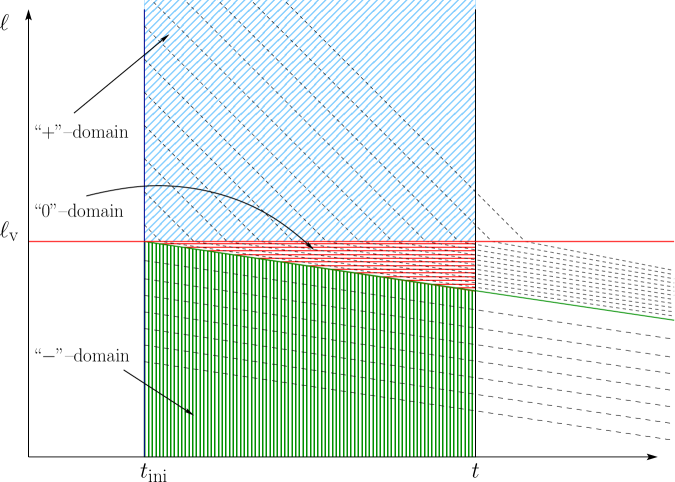
Figure 1: Characteristics $\xi(\ell_{\mathrm{ini}},t)$ of the Liouville operator at fixed $N$ in the plane $(t,\ell)$. At any time $t$, the Cauchy problem is solved by specifying initial conditions on the surface $t=t_{\mathrm{ini}}$ and propagating them along the characteristics in the “+” and “–” regions. Notice that the solution in the “0” region is determined by specifying initial condition on the line $\ell=\ell_{\mathrm{v}}$, which can still be deduced from $t=t_{\mathrm{ini}}$ after evolution through the “+” domain.

2.3.1 Jacobian

In order to determine $\mathcal{J}(\ell,t)$, the function $\xi(\ell_{\mathrm{ini}},t)$ is needed. Integrating Eq. (2.3) gives

$$\xi(\ell_{\mathrm{ini}},t) =\Theta\negthinspace\left(\ell_{\mathrm{v}}-\ell_{\mathrm{ini}}\right)\left(\ell_{\mathrm{ini}}-\gamma_{\mathrm{v}}t\right)+\Theta\negthinspace\left(\ell_{\mathrm{ini}}-\ell_{\mathrm{v}}\right)\bigg{\{}\left(\ell_{\mathrm{ini}}-\gamma_{\mathrm{d}}t\right)\Theta\negthinspace\left(\ell_{\mathrm{ini}}-\ell_{\mathrm{v}}-\gamma_{\mathrm{d}}t\right)$$ (2.11)

$$+\left[\ell_{\mathrm{v}}-\gamma_{\mathrm{v}}t+\dfrac{\gamma_{\mathrm{v}}}{\gamma_{\mathrm{d}}}\left(\ell_{\mathrm{ini}}-\ell_{\mathrm{v}}\right)\right]\Theta\negthinspace\left(\gamma_{\mathrm{d}}t+\ell_{\mathrm{v}}-\ell_{\mathrm{ini}}\right)\bigg{\}},$$

from which we deduce that

$$\dfrac{\partial\xi}{\partial\ell_{\mathrm{ini}}}(\ell_{\mathrm{ini}},t)=\Theta\negthinspace\left(\ell_{\mathrm{v}}-\ell_{\mathrm{ini}}\right)+\Theta\negthinspace\left(\ell_{\mathrm{ini}}-\ell_{\mathrm{v}}\right)\left[\Theta\negthinspace\left(\ell_{\mathrm{ini}}-\ell_{\mathrm{v}}-\gamma_{\mathrm{d}}t\right)+\dfrac{\gamma_{\mathrm{v}}}{\gamma_{\mathrm{d}}}\Theta\negthinspace\left(\gamma_{\mathrm{d}}t+\ell_{\mathrm{v}}-\ell_{\mathrm{ini}}\right)\right],$$ (2.12)

where we have set $t_{\mathrm{ini}}=0$.

The Jacobian $\mathcal{J}(\ell,t)$ is obtained by taking the modulus of the above equation, up to a change of variables $(\ell_{\mathrm{ini}},t)\rightarrow(\ell,t)$. This requires the inversion of Eq. (2.11) to get $\ell_{\mathrm{ini}}=\xi^{-1}(\ell,t)$. After some algebra, the final expression simplifies considerably and reads

$$\mathcal{J}(\ell,t)=\Theta\negthinspace\left(\ell-\ell_{\mathrm{v}}\right)+\Theta\negthinspace\left(\ell_{\mathrm{v}}-\ell\right)\left[\Theta\negthinspace\left(\ell_{\mathrm{v}}-\ell-\gamma_{\mathrm{v}}t\right)+\dfrac{\gamma_{\mathrm{v}}}{\gamma_{\mathrm{d}}}\Theta\negthinspace\left(\ell+\gamma_{\mathrm{v}}t-\ell_{\mathrm{v}}\right)\right],$$ (2.13)

which merely reflects the changes of slopes of the decaying processes (see Fig. 1 discussed below). At any time $t$ and for any value of $N$, the Jacobian is unity for all loop sizes satisfying $\ell>\ell_{\mathrm{v}}(N)$. It then switches to the value $\gamma_{\mathrm{v}}/\gamma_{\mathrm{d}}$ in the domain $\ell_{\mathrm{v}}-\gamma_{\mathrm{v}}t<\ell<\ell_{\mathrm{v}}$ and returns to one again for $\ell<\ell_{\mathrm{v}}-\gamma_{\mathrm{v}}t$. Fig. 1 shows these three domains in the $(t,\ell)$ plane, respectively denoted as “+”, “0” and “–”. Their origin lies in the various histories a $\ell_{\mathrm{ini}}$-sized loop starting at $t=t_{\mathrm{ini}}$ may have. From Eq. (2.11), all loops starting with $\ell_{\mathrm{ini}}<\ell_{\mathrm{v}}$ (“–” domain) decay with a rate given by $\gamma_{\mathrm{v}}$ as being already centrifugally supported. The loop number density distribution per $\Delta\ell$ interval is thus preserved and the Jacobian is unity. At any time $t$, all loops having $\ell>\ell_{\mathrm{v}}$ are necessarily coming from $\ell_{\mathrm{ini}}>\ell_{\mathrm{v}}$. Since they never crossed $\ell_{\mathrm{v}}$, they have shrunk only by gravitational radiation, again at a constant rate given by $\gamma_{\mathrm{d}}$, the Jacobian is also equal to unity. Only the loops in the “0” domain have a two steps history. They started with $\ell_{\mathrm{ini}}>\ell_{\mathrm{v}}$, then radiated gravitational waves until they became vortons by hitting $\ell=\ell_{\mathrm{v}}$. Once vortonized, their energy emission rate being $\gamma_{\mathrm{v}}\ll\gamma_{\mathrm{d}}$, they start accumulating in this region and the Jacobian takes the value $\gamma_{\mathrm{v}}/\gamma_{\mathrm{d}}\ll 1$.

2.3.2 Loop number density distribution

We are now in the position to solve Eq. (2.7) without the collision term, i.e. in absence of loop production. This is a first order differential equation whose characteristics are given by Eq. (2.11).

Figure 2: Liouville time evolution of the loop distribution given by Eqs. (2.19), (2.22) and (2.24) with $\gamma_{\mathrm{d}}=1$. At $t=t_{\mathrm{ini}}$, we assume a gaussian initial distribution centered at $\ell=\ell_{\mathrm{p}}=5$ with a standard deviation of $\sigma_{\mathrm{p}}=1$ (full black line). We also assumed perfectly stable vortons, so that $\gamma_{\mathrm{v}}=0$, and we smoothed the step function appearing in Eq.(2.3) with $\Theta(\ell-\ell_{\mathrm{v}})\to\left\{1+\tanh\left[(\ell-\ell_{\mathrm{v}})/\lambda\right]\right\}/2$, and $\lambda=0.5$: this is the reason why the distribution is non-vanishing for values of $\ell$ smaller than $\ell_{\mathrm{v}}$. As time evolves, the distribution is shifted to the left, where it starts rapidly feeling the vorton characteristic scale $\ell_{\mathrm{v}}$, here numerically set to $2$. Each curve represents the distribution one unit of time after the previous curve, i.e., in the units used, the initial gaussian is for $t=0$, and then $t=1,2,\dots,8$ (orange dotted, pink dashed, and so on, respectively). As time passes, the distribution evolves to a very sharp peak located around $\ell_{\mathrm{v}}$, which gives a Dirac distribution $\delta(\ell-\ell_{\mathrm{v}})$ in the limit $\lambda\to 0$.

According to the values of $\ell$, it is convenient to introduce the new coordinates $(\tau,x)$ and $(\tau,y)$ defined as

$$\forall\ell>\ell_{\mathrm{v}}(N) \quad\Rightarrow\quad\tau\equiv t,\quad x\equiv\gamma_{\mathrm{d}}t+\ell\,,$$ (2.14)

$$\forall\ell<\ell_{\mathrm{v}}(N) \quad\Rightarrow\quad\tau\equiv t,\quad y\equiv\gamma_{\mathrm{v}}t+\ell\,.$$

In terms of these variables, the Liouville equation, i.e. Eq. (2.7) with $\mathcal{P}(\ell,t)=0$, takes the simple form

$$\dfrac{\partial(a^{3}\mathcal{F})}{\partial\tau}=0\,.$$ (2.15)

The solutions are

$$a^{3}(t)\mathcal{F}(t,\ell>\ell_{\mathrm{v}},N) =I(\ell+\gamma_{\mathrm{d}}t,N),$$ (2.16)

$$a^{3}(t)\mathcal{F}(t,\ell<\ell_{\mathrm{v}},N) =J(\ell+\gamma_{\mathrm{v}}t,N),$$

where $I(\cdot,\cdot)$ and $J(\cdot,\cdot)$ are two arbitrary functions still to be determined. Given the loop distribution at some initial time $t_{\mathrm{ini}}$,

$$\dfrac{\partial^{2}n}{\partial\ell\partial N}(t_{\mathrm{ini}},\ell,N)=\mathcal{N}_{\mathrm{ini}}(\ell,N)\,,$$ (2.17)

one can determine these two functions in their respective domain of definition. Plugging Eq. (2.16) into Eq. (2.17) and making use of Eqs. (2.8) and (2.13), all evaluated at $t=t_{\mathrm{ini}}$ gives

$$I(z>z_{\mathrm{ini}},N)=a_{\mathrm{ini}}^{3}\mathcal{N}_{\mathrm{ini}}(z-\gamma_{\mathrm{d}}t_{\mathrm{ini}},N),$$ (2.18)

where $z_{\mathrm{ini}}\equiv\ell_{\mathrm{v}}+\gamma_{\mathrm{d}}t_{\mathrm{ini}}$. This expression completely fixes the solution inside the “+” domain as

$$a^{3}(t)\dfrac{\partial^{2}n}{\partial\ell\partial N}(t,\ell,N)=a_{\mathrm{ini}}^{3}\mathcal{N}_{\mathrm{ini}}\negthinspace\left[\ell+\gamma_{\mathrm{d}}(t-t_{\mathrm{ini}}),N\right],$$ (2.19)

$$\ell>\ell_{\mathrm{v}}(N).$$

According to the discussion of the previous section, the solution in the “0” domain is uniquely determined by propagating this solution to $\ell=\ell_{\mathrm{v}}$, at all times. The matching condition implies

$$a_{\mathrm{ini}}^{3}\mathcal{N}_{\mathrm{ini}}\negthinspace\left[\ell_{\mathrm{v}}+\gamma_{\mathrm{d}}(t-t_{\mathrm{ini}}),N\right]=J(\ell_{\mathrm{v}}+\gamma_{\mathrm{v}}t,N),$$ (2.20)

such that

$$J(z>z_{\mathrm{v}},N)=a_{\mathrm{ini}}^{3}\mathcal{N}_{\mathrm{ini}}\negthinspace\left[\ell_{\mathrm{v}}+\dfrac{\gamma_{\mathrm{d}}}{\gamma_{\mathrm{v}}}\left(z-\ell_{\mathrm{v}}\right)-\gamma_{\mathrm{d}}t_{\mathrm{ini}},N\right].$$ (2.21)

Here, we have defined $z_{\mathrm{v}}\equiv\ell_{\mathrm{v}}+\gamma_{\mathrm{v}}t_{\mathrm{ini}}$. Plugging this expression back into Eq. (2.16), restricted on $\ell+\gamma_{\mathrm{v}}t>z_{\mathrm{v}}$ (and $\ell<\ell_{\mathrm{v}}$) completely fixes the solution inside the “0” domain

$$a^{3}(t)\dfrac{\partial^{2}n}{\partial\ell\partial N}(t,\ell,N)=a_{\mathrm{ini}}^{3}\dfrac{\gamma_{\mathrm{d}}}{\gamma_{\mathrm{v}}}\mathcal{N}_{\mathrm{ini}}\negthinspace\left[\ell_{\mathrm{v}}+\dfrac{\gamma_{\mathrm{d}}}{\gamma_{\mathrm{v}}}\left(\ell-\ell_{\mathrm{v}}\right)+\gamma_{\mathrm{d}}\left(t-t_{\mathrm{ini}}\right),N\right],$$ (2.22)

$$\ell_{\mathrm{v}}(N)-\gamma_{\mathrm{v}}(t-t_{\mathrm{ini}})<\ell<\ell_{\mathrm{v}}(N)\,.$$

At that point, $J(z,N)$ is not yet determined for $z<z_{\mathrm{v}}$. However, this part is exactly the “–” domain for which the initial conditions are fixed at $t=t_{\mathrm{ini}}$ and

$$J(z<z_{\mathrm{v}},N)=a_{\mathrm{ini}}^{2}\mathcal{N}_{\mathrm{ini}}(z-\gamma_{\mathrm{v}}t_{\mathrm{ini}},N).$$ (2.23)

The solution finally reads

$$a^{3}(t)\dfrac{\partial^{2}n}{\partial\ell\partial N}(t,\ell,N)=a_{\mathrm{ini}}^{3}\mathcal{N}_{\mathrm{ini}}\negthinspace\left[\ell+\gamma_{\mathrm{v}}(t-t_{\mathrm{ini}}),N\right],$$ (2.24)

$$\ell<\ell_{\mathrm{v}}(N)-\gamma_{\mathrm{v}}(t-t_{\mathrm{ini}}).$$

The loop distribution at all times $t>t_{\mathrm{ini}}$, length $\ell$ and conserved quantum number $N$ is then given by the set of Eqs. (2.19), (2.22) and (2.24). Although the solutions in region “+” and “–” could have been intuitively guessed as they only shift the initial loop distribution according to the gravitational and vortonic energy emission rates, Eq. (2.22) shows that loops tend to accumulate into the region “0”.

This is exemplified on Fig.2, showing the time evolution of an initially gaussian distribution and producing perfectly stable vortons, case to which we now turn.

2.3.3 Perfectly stable vortons

In the limit of perfectly stable vortons, i.e. $\gamma_{\mathrm{v}}\rightarrow 0$, Eq. (2.22) is singular and the loop density distribution becomes infinite but into a phase space region which becomes infinitely small (see Fig. 1). This is not problematic as the physical quantity of interest is the total number of loop in that region. We can therefore define the number of “vortons” having a charge $N$, at time $t$ by

$$\mathcal{V}_{\mathrm{ini}}(t,N)\equiv\int_{\ell_{\mathrm{v}}-\gamma_{\mathrm{v}}(t-t_{\mathrm{ini}})}^{\ell_{\mathrm{v}}}\negthickspace\dfrac{\partial^{2}n}{\partial\ell\partial N}(t,\ell,N)\,\mathrm{d}\ell\,,$$ (2.25)

where “ini” is a reminder that, in absence of loop production, they can only come from the initial loop distribution. Using Eq. (2.22), defining for each time slice the new variable

$$\sigma\equiv\dfrac{\gamma_{\mathrm{d}}}{\gamma_{\mathrm{v}}}\left(\ell-\ell_{\mathrm{v}}\right)+\gamma_{\mathrm{d}}(t-t_{\mathrm{ini}}),$$ (2.26)

the integral reduces to

$$\mathcal{V}_{\mathrm{ini}}(t,N)=\dfrac{a_{\mathrm{ini}}^{3}}{a^{3}(t)}\int_{0}^{\gamma_{\mathrm{d}}(t-t_{\mathrm{ini}})}\mathcal{N}_{\mathrm{ini}}(\ell_{\mathrm{v}}+\sigma,N)\mathrm{d}\sigma\,,$$ (2.27)

which is well-defined and finite. For an homogeneous initial distribution ($\mathcal{N}_{\mathrm{ini}}=\mathrm{C}^{\mathrm{te}}$) one recovers the intuitive result that the number of vortons grows linearly with time as $a^{3}\mathcal{V}_{\mathrm{ini}}\propto\gamma_{\mathrm{d}}(t-t_{\mathrm{ini}})$.

We conclude that, in the limit of perfectly stable vortons $\gamma_{\mathrm{v}}\rightarrow 0$, the loop density distribution reads, for all $\ell$,

$$\lim_{\gamma_{\mathrm{v}}\rightarrow 0}a^{3}(t)\dfrac{\partial^{2}n}{\partial\ell\partial N}(t,\ell,N) =\Theta\negthinspace\left(\ell_{\mathrm{v}}-\ell\right)a_{\mathrm{ini}}^{3}\mathcal{N}_{\mathrm{ini}}(\ell,N)$$ (2.28)

$$+\Theta\negthinspace\left(\ell-\ell_{\mathrm{v}}\right)a_{\mathrm{ini}}^{3}\mathcal{N}_{\mathrm{ini}}\negthinspace\left[\ell+\gamma_{\mathrm{d}}\left(t-t_{\mathrm{ini}}\right),N\right]$$

$$+\delta\negthinspace\left(\ell-\ell_{\mathrm{v}}\right)a_{\mathrm{ini}}^{3}\int_{0}^{\gamma_{\mathrm{d}}(t-t_{\mathrm{ini}})}\mathcal{N}_{\mathrm{ini}}(\ell_{\mathrm{v}}+\sigma,N)\mathrm{d}\sigma\,.$$

2.4 Boltzmann evolution with loop production

We now solve Eq. (2.7) in full generality by separating the phase space into the same three domains.

2.4.1 Formal solution

For all $\ell>\ell_{\mathrm{v}}(N)$, Eq. (2.7) can be recast in terms of the variable $(\tau,x)$ introduced in Eq. (2.14) as

$$\dfrac{\partial\left(a^{3}\mathcal{F}\right)}{\partial\tau}=a^{3}(\tau)\mathcal{P}(x-\gamma_{\mathrm{d}}\tau,\tau)\delta\negthinspace\left(N-\sqrt{\dfrac{x-\gamma_{\mathrm{d}}\tau}{\lambda}}\right),$$ (2.29)

the Jacobian being unity there. The delta function has an argument depending on $\tau$ such that it simplifies to

$$\delta\negthinspace\left(N-\sqrt{\dfrac{x-\gamma_{\mathrm{d}}\tau}{\lambda}}\right)=\dfrac{2\ell_{\mathrm{p}}(N)}{N\gamma_{\mathrm{d}}}\,\delta\negthinspace\left[\tau-\tau_{\mathrm{p}}(x,N)\right],$$ (2.30)

where $\ell_{\mathrm{p}}(N)$ is given by Eq. (2.9) and

$$\tau_{\mathrm{p}}(x,N)\equiv\dfrac{x-\ell_{\mathrm{p}}(N)}{\gamma_{\mathrm{d}}}\,.$$ (2.31)

The loop distribution in the “+” domain is then solution of

$$\dfrac{\partial\left(a^{3}\mathcal{F}\right)}{\partial\tau}=2a^{3}[\tau_{\mathrm{p}}(x,N)]\,\dfrac{\ell_{\mathrm{p}}(N)}{\gamma_{\mathrm{d}}N}\,\mathcal{P}[\ell_{\mathrm{p}}(N),\tau_{\mathrm{p}}(x,N)]\,\delta\negthinspace\left[\tau-\tau_{\mathrm{p}}(x,N)\right],$$ (2.32)

and reads

$$a^{3}\mathcal{F}(\tau,x,N)=I(x,N)+2a^{3}[\tau_{\mathrm{p}}(x,N)]\,\dfrac{\ell_{\mathrm{p}}(N)}{\gamma_{\mathrm{d}}N}\,\mathcal{P}[\ell_{\mathrm{p}}(N),\tau_{\mathrm{p}}(x,N)]\,\Theta\negthinspace\left[\tau-\tau_{\mathrm{p}}(x,N)\right].$$ (2.33)

As for the Liouville equation, $I(x,N)$ is a unknown function that has to be determined from the initial conditions. In terms of the original variables, the previous equation reads

$$a^{3}\dfrac{\partial^{2}n}{\partial\ell\partial N}(t,\ell,N) =I(\ell+\gamma_{\mathrm{d}}t,N)$$ (2.34)

$$+\dfrac{2\ell_{\mathrm{p}}}{\gamma_{\mathrm{d}}N}\,a^{3}\negthinspace\left(t+\dfrac{\ell-\ell_{\mathrm{p}}}{\gamma_{\mathrm{d}}}\right)\mathcal{P}\negthinspace\left(\ell_{\mathrm{p}},t+\dfrac{\ell-\ell_{\mathrm{p}}}{\gamma_{\mathrm{d}}}\right)\Theta\negthinspace\left(\ell_{\mathrm{p}}-\ell\right),$$

$$\ell>\ell_{\mathrm{v}}(N).$$

For all $\ell<\ell_{\mathrm{v}}(N)$, we can similarly use the new variables $(\tau,y)$ defined in Eq. (2.14) to solve Eq. (2.7). In fact, since $\ell_{\mathrm{p}}\gg\ell_{\mathrm{v}}$ (or null), the source term always vanish in that domain and the solution is the same as in Sec. 2.3, i.e.

$$a^{3}\mathcal{J}(\ell,t)\dfrac{\partial^{2}n}{\partial\ell\partial N}(t,\ell,N)=J(\ell+\gamma_{\mathrm{v}}t,N),$$ (2.35)

$$\ell<\ell_{\mathrm{v}}(N),$$

where the function $J(z,N)$ has again to be determined from the initial conditions. Notice that the Jacobian $\mathcal{J}(\ell,t)$ is either unity or equal to $\gamma_{\mathrm{v}}/\gamma_{\mathrm{d}}$ according to the domain “–” or “0”, respectively. The formal solution is therefore given by both Eqs. (2.34) and (2.35).

2.4.2 Full solution from specified initial conditions

As for the Liouville equation, we assume the loop distribution to be known at some initial time $t_{\mathrm{ini}}$ and given by Eq. (2.17).

For all $\ell>\ell_{\mathrm{v}}$, i.e. in the “+” domain, Eq. (2.34) evaluated at $t=t_{\mathrm{ini}}$ fixes the function

$$I(z>z_{\mathrm{ini}},N)=a_{\mathrm{ini}}^{3}\mathcal{N}_{\mathrm{ini}}(z-\gamma_{\mathrm{d}}t_{\mathrm{ini}},N)-\dfrac{2\ell_{\mathrm{p}}}{\gamma_{\mathrm{d}}N}a^{3}\negthinspace\left(\dfrac{z-\ell_{\mathrm{p}}}{\gamma_{\mathrm{d}}}\right)\times\Theta\negthinspace\left(t_{\mathrm{ini}}+\dfrac{\ell_{\mathrm{p}}-z}{\gamma_{\mathrm{d}}}\right)\mathcal{P}\negthinspace\left(\ell_{\mathrm{p}},\dfrac{z-\ell_{\mathrm{p}}}{\gamma_{\mathrm{d}}}\right),$$ (2.36)

where $z_{\mathrm{ini}}=\ell_{\mathrm{v}}+\gamma_{\mathrm{d}}t_{\mathrm{ini}}$. Notice that the Heaviside function ensures that the argument of the scale factor $a(\cdot)$ is always larger or equal than $t_{\mathrm{ini}}$. Plugging $I(z,N)$, back into Eq. (2.34) gives the wanted result

$$\begin{aligned} a^{3}(t)\dfrac{\partial^{2}n}{\partial\ell\partial N}(t,\ell,N)&=a_{\mathrm{ini}}^{3}\mathcal{N}_{\mathrm{ini}}\negthinspace\left[\ell+\gamma_{\mathrm{d}}(t-t_{\mathrm{ini}}),N\right]+\dfrac{2\ell_{\mathrm{p}}}{\gamma_{\mathrm{d}}N}a^{3}\negthinspace\left(t-\dfrac{\ell_{\mathrm{p}}-\ell}{\gamma_{\mathrm{d}}}\right)\\ &\times\mathcal{P}\negthinspace\left(\ell_{\mathrm{p}},t-\dfrac{\ell_{\mathrm{p}}-\ell}{\gamma_{\mathrm{d}}}\right)\Big{\{}\Theta\negthinspace\left(\ell_{\mathrm{p}}-\ell\right)-\Theta\negthinspace\left[\ell_{\mathrm{p}}-\ell-\gamma_{\mathrm{d}}(t-t_{\mathrm{ini}})\right]\Big{\}},\end{aligned}$$ (2.37)

$$\ell>\ell_{\mathrm{v}}(N).$$

For all $\ell<\ell_{\mathrm{v}}(N)$, we start from the solution (2.35). However, as in Sec. 2.3, there are two sub-cases corresponding to the domain “0” and “–” of Fig. 1.

On one hand, for $\ell_{\mathrm{v}}-\gamma_{\mathrm{v}}(t-t_{\mathrm{ini}})<\ell<\ell_{\mathrm{v}}$, we determine the $J$ function by matching Eq. (2.35) to Eq. (2.37) at $\ell=\ell_{\mathrm{v}}$ and for all times. One gets

$$J(z >z_{\mathrm{v}},N)=a_{\mathrm{ini}}^{3}\mathcal{N}_{\mathrm{ini}}\negthinspace\left[\ell_{\mathrm{v}}+\dfrac{\gamma_{\mathrm{d}}}{\gamma_{\mathrm{v}}}(z-\ell_{\mathrm{v}})-\gamma_{\mathrm{d}}t_{\mathrm{ini}},N\right]+\dfrac{2\ell_{\mathrm{p}}}{\gamma_{\mathrm{d}}N}a^{3}\negthinspace\left(\dfrac{z-\ell_{\mathrm{v}}}{\gamma_{\mathrm{v}}}-\dfrac{\ell_{\mathrm{p}}-\ell_{\mathrm{v}}}{\gamma_{\mathrm{d}}}\right)$$ (2.38)

$$\times \mathcal{P}\negthinspace\left(\ell_{\mathrm{p}},\dfrac{z-\ell_{\mathrm{v}}}{\gamma_{\mathrm{v}}}-\dfrac{\ell_{\mathrm{p}}-\ell_{\mathrm{v}}}{\gamma_{\mathrm{d}}}\right)\left[\Theta\negthinspace\left(\dfrac{\ell_{\mathrm{p}}-\ell_{\mathrm{v}}}{\gamma_{\mathrm{d}}}\right)-\Theta\negthinspace\left(t_{\mathrm{ini}}+\dfrac{\ell_{\mathrm{p}}-\ell_{\mathrm{v}}}{\gamma_{\mathrm{d}}}-\dfrac{z-\ell_{\mathrm{v}}}{\gamma_{\mathrm{v}}}\right)\right],$$

where, as before, $z_{\mathrm{v}}=\ell_{\mathrm{v}}+\gamma_{\mathrm{v}}t_{\mathrm{ini}}$. This completely fixes the solution in the “0” domain which reads

$$\begin{aligned} a^{3}(t)\dfrac{\partial^{2}n}{\partial\ell\partial N}(t,\ell,N)&=a_{\mathrm{ini}}^{3}\dfrac{\gamma_{\mathrm{d}}}{\gamma_{\mathrm{v}}}\mathcal{N}_{\mathrm{ini}}\negthinspace\left[\ell_{\mathrm{v}}+\dfrac{\gamma_{\mathrm{d}}}{\gamma_{\mathrm{v}}}(\ell-\ell_{\mathrm{v}})+\gamma_{\mathrm{d}}(t-t_{\mathrm{ini}}),N\right]\\ &+\dfrac{2\ell_{\mathrm{p}}}{\gamma_{\mathrm{v}}N}a^{3}\negthinspace\left(t-\dfrac{\ell_{\mathrm{v}}-\ell}{\gamma_{\mathrm{v}}}-\dfrac{\ell_{\mathrm{p}}-\ell_{\mathrm{v}}}{\gamma_{\mathrm{d}}}\right)\mathcal{P}\negthinspace\left(\ell_{\mathrm{p}},t-\dfrac{\ell_{\mathrm{v}}-\ell}{\gamma_{\mathrm{v}}}-\dfrac{\ell_{\mathrm{p}}-\ell_{\mathrm{v}}}{\gamma_{\mathrm{d}}}\right)\\ &\times\left\{\Theta\negthinspace\left(\ell_{\mathrm{p}}-\ell_{\mathrm{v}}\right)-\Theta\negthinspace\left[\ell_{\mathrm{p}}-\ell_{\mathrm{v}}+\dfrac{\gamma_{\mathrm{d}}}{\gamma_{\mathrm{v}}}(\ell_{\mathrm{v}}-\ell)-\gamma_{\mathrm{d}}(t-t_{\mathrm{ini}})\right]\right\},\end{aligned}$$ (2.39)

$$\ell_{\mathrm{v}}(N)-\gamma_{\mathrm{v}}(t-t_{\mathrm{ini}})<\ell<\ell_{\mathrm{v}}(N).$$

Notice that the Heaviside function $\Theta\negthinspace\left(\ell_{\mathrm{p}}-\ell_{\mathrm{v}}\right)=1$ under our hypothesis $\ell_{\mathrm{p}}\gg\ell_{\mathrm{v}}$.

On the other hand, when $\ell<\ell_{\mathrm{v}}-\gamma_{\mathrm{v}}(t-t_{\mathrm{ini}})$, the function $J(z<z_{\mathrm{v}},N)$ is set by the initial loop distribution at $t=t_{\mathrm{ini}}$. Since the source terms vanish in that region, combining Eqs. (2.17) and (2.35) yields exactly Eq. (2.23) for $J$. As a result, the loop distribution in that domain is the same as the one derived from the Liouville operator in Eq. (2.24).

To summarize, starting from the initial distribution of Eq. (2.17), in presence of a loop production function, the loop number density distribution at time $t$, for all $\ell$ and $N$ is given by Eqs. (2.37), (2.39) and (2.24).

2.4.3 Perfectly stable vortons with loops production

As for the Liouville solution, our results also apply to the particular limit $\gamma_{\mathrm{v}}\rightarrow 0$. The number of vortons can be defined as in Eq. (2.25) and is obtained by integrating Eq. (2.39) over all loop sizes intercepting the “0” domain at time $t$. The first term is the same as in Eq. (2.27) while there is an additional contribution coming from the loop production function. Defining

$$t_{\mathrm{p}\mathrm{v}}(N)\equiv\dfrac{\ell_{\mathrm{p}}(N)-\ell_{\mathrm{v}}(N)}{\gamma_{\mathrm{d}}}=\dfrac{N}{\gamma_{\mathrm{d}}}\left(\lambda N-\dfrac{1}{\sqrt{U}}\right),$$ (2.40)

the time required for a loop of size $\ell_{\mathrm{p}}(N)$ to reach $\ell_{\mathrm{v}}(N)$ by gravitational radiation, and the new variable

$$\varsigma\equiv\dfrac{\ell-\ell_{\mathrm{v}}}{\gamma_{\mathrm{v}}}+t\,,$$ (2.41)

one gets

$$\mathcal{V}(t,N)=\mathcal{V}_{\mathrm{ini}}(t,N)+\dfrac{2\ell_{\mathrm{p}}}{a^{3}(t)N}\int_{t_{\mathrm{ini}}}^{t}a^{3}(\varsigma-t_{\mathrm{p}\mathrm{v}})\mathcal{P}(\ell_{\mathrm{p}},\varsigma-t_{\mathrm{p}\mathrm{v}})\Theta\negthinspace\left(\varsigma-t_{\mathrm{p}\mathrm{v}}\right)\mathrm{d}\varsigma\,.$$ (2.42)

This expression does no longer depend on $\gamma_{\mathrm{v}}$ which makes it valid even for $\gamma_{\mathrm{v}}\rightarrow 0$. It shows that, in addition to the vortons coming from the initial loop distribution, loop production incessantly feeds the vortons reservoir with a time delay given by $t_{\mathrm{p}\mathrm{v}}(N)$.

The loop distribution when $\gamma_{\mathrm{v}}\rightarrow 0$, in presence of a loop production function, finally reads for all $\ell$:

$$\lim_{\gamma_{\mathrm{v}}\rightarrow 0}a^{3}(t)\dfrac{\partial^{2}n}{\partial\ell\partial N}(t,\ell,N) =\Theta\negthinspace\left(\ell_{\mathrm{v}}-\ell\right)a_{\mathrm{ini}}^{3}\mathcal{N}_{\mathrm{ini}}(\ell,N)$$ (2.43)

$$+\Theta\negthinspace\left(\ell-\ell_{\mathrm{v}}\right)a_{\mathrm{ini}}^{3}\mathcal{N}_{\mathrm{ini}}\negthinspace\left[\ell+\gamma_{\mathrm{d}}\left(t-t_{\mathrm{ini}}\right),N\right]$$

$$+\Theta\negthinspace\left(\ell-\ell_{\mathrm{v}}\right)\dfrac{2\ell_{\mathrm{p}}}{\gamma_{\mathrm{d}}N}a^{3}\negthinspace\left(t-\dfrac{\ell_{\mathrm{p}}-\ell}{\gamma_{\mathrm{d}}}\right)\mathcal{P}\negthinspace\left(\ell_{\mathrm{p}},t-\dfrac{\ell_{\mathrm{p}}-\ell}{\gamma_{\mathrm{d}}}\right)$$

$$\times\Big{\{}\Theta\negthinspace\left(\ell_{\mathrm{p}}-\ell\right)-\Theta\negthinspace\left[\ell_{\mathrm{p}}-\ell-\gamma_{\mathrm{d}}(t-t_{\mathrm{ini}})\right]\Big{\}}$$

$$+\delta\negthinspace\left(\ell-\ell_{\mathrm{v}}\right)a_{\mathrm{ini}}^{3}\int_{0}^{\gamma_{\mathrm{d}}(t-t_{\mathrm{ini}})}\mathcal{N}_{\mathrm{ini}}(\ell_{\mathrm{v}}+\sigma,N)\mathrm{d}\sigma$$

$$+\delta\negthinspace\left(\ell-\ell_{\mathrm{v}}\right)\dfrac{2\ell_{\mathrm{p}}}{N}\int_{t_{\mathrm{ini}}}^{t}a^{3}(\varsigma-t_{\mathrm{p}\mathrm{v}})\mathcal{P}(\ell_{\mathrm{p}},\varsigma-t_{\mathrm{p}\mathrm{v}})\Theta\negthinspace\left(\varsigma-t_{\mathrm{p}\mathrm{v}}\right)\mathrm{d}\varsigma\,.$$

Note that the initial loop distribution is already responsible for the so-called vorton excess problem, and we are adding a possibly larger term to it: as expected, looking in details at the loop distribution evolution constrains the models even more. We now turn to this question in the relevant cosmological framework.

3 Application to the vorton excess problem

In Ref. [66], the relic abundance of vortons was estimated by assuming that loops are first formed during the string forming phase transition whereas they develop a current at a later time. Under some reasonable assumptions, Ref. [66] approximates the number density of vortons by $n_{\mathrm{v}}\propto n_{\mathrm{f}}(a_{\mathrm{f}}/a)^{3}$ with $n_{\mathrm{f}}\propto 1/L_{\mathrm{f}}^{3}$ denoting the vorton abundance at formation if their distribution peaks around a particular length scale $L_{\mathrm{f}}$. As we show below, our Boltzmann treatment allows to derive the complete current-carrying loop distribution without making assumption on their initial distribution.

Under the same assumptions as in Ref. [66], we assume that loops are formed at an energy scale $T_{\mathrm{x}}\simeq\sqrt{U}$ whereas the current-carrier condensation occurs at the lower temperature $T_{\mathrm{cur}}\simeq\lambda^{-1}$. From the results of Sec. 2, we can readily write down the loop distribution at the time the strings become superconducting, i.e. at $t=t_{\mathrm{cur}}$:

$$\bar{\mathcal{N}}_{\mathrm{cur}}(\ell)=\dfrac{a_{\mathrm{ini}}^{3}}{a^{3}(t_{\mathrm{cur}})}\bar{\mathcal{N}}_{\mathrm{ini}}[\ell+\gamma_{\mathrm{d}}(t_{\mathrm{cur}}-t_{\mathrm{ini}})],$$ (3.1)

where

$$\bar{\mathcal{N}}_{\alpha}\equiv\dfrac{\partial n}{\partial\ell}(\ell,t_{\alpha}),$$ (3.2)

is the loop density distribution at $t=t_{\alpha}$. In Eq. (3.1), $\gamma_{\mathrm{d}}$ describes the loop gravitational decay, complemented or not by any other evaporation effects the loops may experience in the friction dominated regime. For simplicity, we will be keeping an unique $\gamma_{\mathrm{d}}$ in the following. At $t=t_{\mathrm{cur}}$, current-carrier condensation occurs and those loops are endowed with the conserved number $N$ induced by thermal fluctuations of wavelength $\lambda=1/T_{\mathrm{cur}}$:

$$\mathcal{N}_{\mathrm{cur}}(\ell,N)=\bar{\mathcal{N}}_{\mathrm{cur}}(\ell)\,\delta\negthinspace\left(N-\sqrt{\dfrac{\ell}{\lambda}}\right).$$ (3.3)

For $\ell>\lambda$, the loops can potentially become stable vortons. One should nevertheless require that $\ell_{\mathrm{v}}(N)=N/\sqrt{U}>\lambda$, i.e.

$$N>N_{*}\equiv\lambda\sqrt{U}\,.$$ (3.4)

In the opposite situation, $N<N_{*}$, one may expect the current to disappear by some quantum processes and these loops are referred to as “doomed”. This effect can be phenomenologically included within our interpretation by assigning a vanishing effective vorton length for those loops, i.e. by imposing $\ell_{\mathrm{v}}(N<N_{*})=0$. For the large enough loops, following the hypothesis of Ref. [66], there is no loop production and the vortons having $\ell_{\mathrm{v}}>\lambda$ are assumed to be perfectly stable $\gamma_{\mathrm{v}}\rightarrow 0$. Under these assumptions, Eq. (2.43) becomes

$$a^{3}\dfrac{\partial^{2}n}{\partial\ell\partial N}(t,\ell,N)=a_{\mathrm{ini}}^{3}\Theta\negthinspace\left[\ell-\ell_{\mathrm{v}}(N)\right]\bar{\mathcal{N}}_{\mathrm{ini}}[\ell+\gamma_{\mathrm{d}}(t-t_{\mathrm{ini}})]\,\delta\negthinspace\left[N-\sqrt{\dfrac{\ell+\gamma_{\mathrm{d}}(t-t_{\mathrm{cur}})}{\lambda}}\right]$$ (3.5)

$$+a_{\mathrm{ini}}^{3}\delta\negthinspace\left[\ell-\ell_{\mathrm{v}}(N)\right]\int_{0}^{\gamma_{\mathrm{d}}(t-t_{\mathrm{cur}})}\negthickspace\bar{\mathcal{N}}_{\mathrm{ini}}\left[\ell_{\mathrm{v}}(N)+\sigma+\gamma_{\mathrm{d}}(t_{\mathrm{cur}}-t_{\mathrm{ini}})\right]\,\delta\negthinspace\left[N-\sqrt{\dfrac{\ell_{\mathrm{v}}(N)+\sigma}{\lambda}}\right]\mathrm{d}\sigma.$$

Integrating this expression over $N$ gives the number density of proto-vortons plus doomed loops (first line) and vortons (second line) of size $\ell$ at time $t$:

$$a^{3}\dfrac{\partial n}{\partial\ell}(t,\ell)=\int_{0}^{\infty}a^{3}\dfrac{\partial^{2}n}{\partial\ell\partial N}(t,\ell,N)\,\mathrm{d}N.$$ (3.6)

Let us start by the number density of vortons. The first Dirac function in the second line of Eq. (3.5) allows to explicitly perform the integration over $N$. One has

$$\delta\negthinspace\left[\ell-\ell_{\mathrm{v}}(N)\right]=\sqrt{U}\,\delta\negthinspace\left(N-\ell\sqrt{U}\right),$$ (3.7)

provided $N>N_{*}$. In the opposite situation, $\ell_{\mathrm{v}}(N)=0$ and the integral vanishes. All in all, one can use the above expression provided $\ell\sqrt{U}>N_{*}$, i.e. for $\ell>\lambda$ as expected. The vorton term now reads

$$a_{\mathrm{ini}}^{3} \Theta\negthinspace\left(\ell-\lambda\right)\sqrt{U}\int_{0}^{\gamma_{\mathrm{d}}(t-t_{\mathrm{cur}})}\bar{\mathcal{N}}_{\mathrm{ini}}\left[\ell+\sigma+\gamma_{\mathrm{d}}(t-t_{\mathrm{cur}})\right]\delta\negthinspace\left(\ell\sqrt{U}-\sqrt{\dfrac{\ell+\sigma}{\lambda}}\right)\mathrm{d}\sigma$$ (3.8)

$$=2a_{\mathrm{ini}}^{3}N_{*}^{2}\dfrac{\ell}{\lambda}\,\Theta\negthinspace\left(\ell-\lambda\right)\Theta\negthinspace\left[\ell_{{\scriptscriptstyle{\mathrm{T}}}}(t)-\ell\right]\,\bar{\mathcal{N}}_{\mathrm{ini}}\negthinspace\left[N_{*}^{2}\dfrac{\ell^{2}}{\lambda}+\gamma_{\mathrm{d}}(t-t_{\mathrm{cur}})\right],$$

where $\ell_{{\scriptscriptstyle{\mathrm{T}}}}(t)$ is an increasing function of time defined by

$$\ell_{{\scriptscriptstyle{\mathrm{T}}}}(t)\equiv\dfrac{\lambda}{2N_{*}^{2}}\left[1+\sqrt{1+4N_{*}^{2}\dfrac{\gamma_{\mathrm{d}}(t-t_{\mathrm{cur}})}{\lambda}}\right].$$ (3.9)

As can be checked in Eq. (3.8), the remaining Dirac function yields a non-vanishing integral provided $\sigma_{0}=\ell(\lambda U\ell-1)$ belongs to the interval $[0,\gamma_{\mathrm{d}}(t-t_{\mathrm{cur}})]$. After some algebra, this ends up being equivalent to the condition $\ell<\ell_{{\scriptscriptstyle{\mathrm{T}}}}(t)$. Physically, this condition simply arises from the time required for a loop of size $\ell$ to shrink down to the vorton length $\ell_{\mathrm{v}}$. The quantity $\ell_{{\scriptscriptstyle{\mathrm{T}}}}(t)$ is also the upper bound of the vorton length spectrum at any time, their size ranging from $\lambda$ to $\ell_{{\scriptscriptstyle{\mathrm{T}}}}(t)$.

Concerning the first line of Eq. (3.5), accounting for proto-vortons and doomed loops, the integral over $N$ can again be performed explicitly owing to the Dirac function. However, one has to distinguish two cases according to the value of $N_{0}=[\ell/\lambda+\gamma_{\mathrm{d}}(t-t_{\mathrm{cur}})/\lambda]^{1/2}$, the zero of the Dirac function argument. Either $N_{0}<N_{*}$ and $\ell_{\mathrm{v}}(N_{0})=0$, or $N_{0}\geq N_{*}$ and $\ell_{\mathrm{v}}(N_{0})=N_{0}/\sqrt{U}$. Again, these conditions can be recast in terms of lengths by defining a new length scale

$$\ell_{*}(t)\equiv\lambda\left[N_{*}^{2}-\gamma_{\mathrm{d}}(t-t_{\mathrm{cur}})\right],$$ (3.10)

which is a decreasing function of time. At any time, all loops having $\ell<\ell_{*}(t)$ are doomed, they are the ones associated with $N<N_{*}$ and will disappear by decay. For those, we have set above $\ell_{\mathrm{v}}=0$ and the Heaviside function in the first line of Eq. (3.5) equals unity. All the others loops, having $\ell>\ell_{*}(t)$ are proto-vortons, i.e. in the shrinking stage before becoming vortons. This can be explicitly seen by rewriting the Heaviside function as

$$\Theta\negthinspace\left[\ell-\ell_{\mathrm{v}}(N_{0})\right]=\Theta\negthinspace\left[\ell_{*}(t)-\ell\right]+\Theta\negthinspace\left[\ell-\ell_{*}(t)\right]\Theta\negthinspace\left[\ell-\ell_{{\scriptscriptstyle{\mathrm{T}}}}(t)\right].$$ (3.11)

Combining all terms together, the loop distribution function finally reads

$$a^{3}(t)\dfrac{\partial n}{\partial\ell}(t,\ell) =a_{\mathrm{ini}}^{3}\left\{\Theta\negthinspace\left[\ell_{*}(t)-\ell\right]+\Theta\negthinspace\left[\ell-\ell_{*}(t)\right]\Theta\negthinspace\left[\ell-\ell_{{\scriptscriptstyle{\mathrm{T}}}}(t)\right]\right\}\bar{\mathcal{N}}_{\mathrm{ini}}\negthinspace\left[\ell+\gamma_{\mathrm{d}}(t-t_{\mathrm{ini}})\right]$$ (3.12)

$$+2a_{\mathrm{ini}}^{3}\,N_{*}^{2}\dfrac{\ell}{\lambda}\,\Theta\negthinspace\left[\ell_{{\scriptscriptstyle{\mathrm{T}}}}(t)-\ell\right]\Theta\negthinspace\left(\ell-\lambda\right)\bar{\mathcal{N}}_{\mathrm{ini}}\negthinspace\left[N_{*}^{2}\dfrac{\ell^{2}}{\lambda}+\gamma_{\mathrm{d}}(t_{\mathrm{cur}}-t_{\mathrm{ini}})\right],$$

where $N_{*}$ is given by Eq. (3.4), $\ell_{{\scriptscriptstyle{\mathrm{T}}}}(t)$ and $\ell_{*}(t)$ being defined in Eqs. (3.9) and (3.10), respectively. As we have just discussed, the second line of this expression accounts for all vortons present at time $t$ while the first describe both proto-vortons and doomed loops. Let us stress that the doomed loops, i.e. the domain $\ell<\ell_{*}(t)$ exists only during a transient period after which they completely disappear. This happens at the time $t=t_{*}$ solution of $\ell_{*}(t_{*})=0$, i.e. for

$$t_{*}=t_{\mathrm{cur}}+\dfrac{N_{*}^{2}}{\gamma_{\mathrm{d}}}\,.$$ (3.13)

The loop distribution of Eq. (3.12) generalizes the approach of Ref. [66] for any initial loop distributions while tracking at all times both the proto-vorton and vorton populations. Taking an initial loop distribution peaked at a particular length gives back the results of Refs. [66, 67] in the asymptotic limit $t\gg t_{*}$ and if we neglect the proto-vortons. As a result, we do not expect significant new constraints to be derived from Eq. (3.12), i.e. in the case of a vanishing loop production function. However, as can be seen from Eq. (2.43), for $\mathcal{P}(\ell,t)\neq 0$, as it is found in the numerical simulations, the vorton population should be significantly enhanced. We let however for a future work the derivation of the associated cosmological constraints.

4 Conclusion

We have presented a new way of treating the vorton excess problem, taking into account in principle any kind of interaction between loops and long strings, and in particular the appearance of an ensemble of vortons or quasi-vortons [66], i.e. loop configurations whose internal structure induces a different, possibly vanishing, decay rate. These vortons could plague GUT models having a cosmic string network building as a consequence of primordial symmetry breaking, i.e., basically all cosmologically-compatible GUT [76, 77]. Indeed, in realistic models, the strings that form are expected to couple to various fields [53], some of which leading to current-carrying vortices [55] in such a way that the strings are no longer Nambu-Goto like as usually assumed [69, 78, 79, 80]. This leads to the formation of very-slowly decaying, or even stable, matter scaling objects dubbed vortons, that can change the subsequent evolution in a drastic way. Up to now, only rough evaluation of their contribution has been proposed using their initial distribution function.

In this work we have gone one step further into understanding in more details the vorton distribution and the relevant cosmological constraints. We have presented a new Boltzmann approach governing the evolution of the number density $n(t,\ell,N)$ of current carrying cosmic string loops. Under some assumptions, we have been able to find an explicit solution starting from any initial distributions and for any given loop production functions: the most general results are given by Eqs. (2.24), (2.37) and (2.39).

We have also shown how this method was extending previous results on the cosmological evolution of vortons in the absence of loop production [66, 67], while remaining perfectly compatible in the appropriate limits. Our results could be readily applied to the loop production function found in Ref. [31, 35, 36] to revisit the vorton constraints in presence of loop production, as should be done in a forthcoming work. Another possible extension could be the determination of a complete analytic loop production function but from a system of Boltzmann equations that would explicitly couple long strings and loops with collision and fragmentation terms. Indeed, much still deserves to be done in this area: even though cosmic strings have long ago been ruled out as the main source of density perturbations, it does not mean that they ought not be used as a very powerful tool to provide constraints on theories otherwise unreachable.

References

- [1] A. A. Fraisse, C. Ringeval, D. N. Spergel, and F. R. Bouchet, Small-Angle CMB Temperature Anisotropies Induced by Cosmic Strings, Phys. Rev. D78 (2008) 043535, [arXiv:0708.1162].
- [2] K. Takahashi et. al., Non-Gaussianity in Cosmic Microwave Background Temperature Fluctuations from Cosmic (Super-)Strings, JCAP 0910 (2009) 003, [arXiv:0811.4698].
- [3] M. Hindmarsh, C. Ringeval, and T. Suyama, The CMB temperature bispectrum induced by cosmic strings, Phys. Rev. D80 (2009) 083501, [arXiv:0908.0432].
- [4] M. Hindmarsh, C. Ringeval, and T. Suyama, The CMB temperature trispectrum of cosmic strings, Phys. Rev. D81 (2010) 063505, [arXiv:0911.1241].
- [5] D. M. Regan and E. P. S. Shellard, Cosmic String Power Spectrum, Bispectrum and Trispectrum, Phys. Rev. D82 (2010) 063527, [arXiv:0911.2491].
- [6] D. Yamauchi, Y. Sendouda, C.-M. Yoo, K. Takahashi, A. Naruko, et. al., Skewness in CMB temperature fluctuations from curved cosmic (super-)strings, JCAP 1005 (2010) 033, [arXiv:1004.0600].
- [7] M. Landriau and E. Shellard, Cosmic String Induced CMB Maps, Phys.Rev. D83 (2011) 043516, [arXiv:1004.2885].
- [8] N. Bevis, M. Hindmarsh, M. Kunz, and J. Urrestilla, CMB power spectra from cosmic strings: predictions for the Planck satellite and beyond, Phys. Rev. D82 (2010) 065004, [arXiv:1005.2663].
- [9] C. Ringeval, Cosmic strings and their induced non-Gaussianities in the cosmic microwave background, Adv. Astron. 2010 (2010) 380507, [arXiv:1005.4842].
- [10] H. Tashiro, E. Sabancilar, and T. Vachaspati, CMB Distortions from Superconducting Cosmic Strings, Phys.Rev. D85 (2012) 103522, [arXiv:1202.2474].
- [11] Y.-F. Cai, E. Sabancilar, D. A. Steer, and T. Vachaspati, Radio Broadcasts from Superconducting Strings, Phys.Rev. D86 (2012) 043521, [arXiv:1205.3170].
- [12] C. Ringeval and F. R. Bouchet, All Sky CMB Map from Cosmic Strings Integrated Sachs-Wolfe Effect, Phys.Rev. D86 (2012) 023513, [arXiv:1204.5041].
- [13] D. Kirzhnits and A. Linde, Macroscopic consequences of the Weinberg model, Phys. Lett. B 42 (Dec., 1972) 471–474.
- [14] T. W. B. Kibble, Topology of cosmic domains and strings., J. Phys. A 9 (1976) 1387–1398.
- [15] C. P. Burgess et. al., The Inflationary Brane-Antibrane Universe, JHEP 07 (2001) 047, [hep-th/0105204].
- [16] S. Sarangi and S. H. H. Tye, Cosmic string production towards the end of brane inflation, Phys. Lett. B536 (2002) 185–192, [hep-th/0204074].
- [17] G. Dvali and A. Vilenkin, Formation and evolution of cosmic D-strings, JCAP 0403 (2004) 010, [hep-th/0312007].
- [18] N. T. Jones, H. Stoica, and S. H. H. Tye, The production, spectrum and evolution of cosmic strings in brane inflation, Phys. Lett. B563 (2003) 6–14, [hep-th/0303269].
- [19] A.-C. Davis and T. Kibble, Fundamental cosmic strings, Contemp. Phys. 46 (Sept., 2005) 313–322, [hep-th/0505050].
- [20] M. Sakellariadou, Cosmic strings, Lect. Notes Phys. 718 (2007) 247–288, [hep-th/0602276].
- [21] M. Sakellariadou, Cosmic Superstrings, Phil. Trans. Roy. Soc. Lond. A366 (2008) 2881–2894, [arXiv:0802.3379].
- [22] E. J. Copeland and T. W. B. Kibble, Cosmic Strings and Superstrings, Proc. Roy. Soc. Lond. A466 (2010) 623–657, [arXiv:0911.1345].
- [23] M. Sakellariadou, Cosmic Strings and Cosmic Superstrings, Nucl. Phys. Proc. Suppl. 192-193 (2009) 68–90, [arXiv:0902.0569].
- [24] A. Albrecht and N. Turok, Evolution of cosmic string networks, Phys. Rev. D40 (Aug., 1989) 973–1001.
- [25] D. P. Bennett and F. R. Bouchet, Cosmic-string evolution, Phys. Rev. Lett. 63 (Dec., 1989) 2776–2779.
- [26] D. P. Bennett and F. R. Bouchet, High-resolution simulations of cosmic-string evolution. I. Network evolution, Phys. Rev. D41 (Apr., 1990) 2408–2433.
- [27] B. Allen and P. Shellard, Cosmic-string evolution - A numerical simulation, Phys. Rev. Lett. 64 (Jan., 1990) 119–122.
- [28] G. R. Vincent, M. Hindmarsh, and M. Sakellariadou, Scaling and small scale structure in cosmic string networks, Phys. Rev. D56 (1997) 637–646, [astro-ph/9612135].
- [29] G. Vincent, N. D. Antunes, and M. Hindmarsh, Numerical Simulations of String Networks in the Abelian-Higgs Model, Phys. Rev. Lett. 80 (Mar., 1998) 2277–2280, [hep-ph/9708427].
- [30] J. N. Moore, E. P. S. Shellard, and C. J. A. P. Martins, Evolution of Abelian-Higgs string networks, Phys. Rev. D65 (Jan., 2001) 023503, [hep-ph/0107171].
- [31] C. Ringeval, M. Sakellariadou, and F. Bouchet, Cosmological evolution of cosmic string loops, JCAP 0702 (2007) 023, [astro-ph/0511646].
- [32] M. Hindmarsh, S. Stuckey, and N. Bevis, Abelian Higgs Cosmic Strings: Small Scale Structure and Loops, Phys. Rev. D79 (2009) 123504, [arXiv:0812.1929].
- [33] J. Urrestilla, N. Bevis, M. Hindmarsh, and M. Kunz, Cosmic string parameter constraints and model analysis using small scale Cosmic Microwave Background data, JCAP 1112 (2011) 021, [arXiv:1108.2730].
- [34] V. Vanchurin, K. Olum, and A. Vilenkin, Cosmic string scaling in flat space, Phys. Rev. D72 (2005) 063514, [gr-qc/0501040].
- [35] J. Polchinski and J. V. Rocha, Analytic study of small scale structure on cosmic strings, Phys. Rev. D74 (2006) 083504, [hep-ph/0606205].
- [36] F. Dubath, J. Polchinski, and J. V. Rocha, Cosmic String Loops, Large and Small, Phys. Rev. D77 (2008) 123528, [arXiv:0711.0994].
- [37] J. V. Rocha, Scaling solution for small cosmic string loops, Phys. Rev. Lett. 100 (2008) 071601, [arXiv:0709.3284].
- [38] V. Vanchurin, K. D. Olum, and A. Vilenkin, Scaling of cosmic string loops, Phys. Rev. D74 (2006) 063527, [gr-qc/0511159].
- [39] C. J. A. P. Martins and E. P. S. Shellard, Fractal properties and small-scale structure of cosmic string networks, Phys. Rev. D73 (2006) 043515, [astro-ph/0511792].
- [40] K. D. Olum and V. Vanchurin, Cosmic string loops in the expanding universe, Phys. Rev. D75 (2007) 063521, [astro-ph/0610419].
- [41] J. J. Blanco-Pillado, K. D. Olum, and B. Shlaer, Large parallel cosmic string simulations: New results on loop production, Phys.Rev. D83 (2011) 083514, [arXiv:1101.5173].
- [42] D. Austin, E. J. Copeland, and T. W. B. Kibble, Evolution of cosmic string configurations, Phys. Rev. D48 (1993) 5594–5627, [hep-ph/9307325].
- [43] C. J. A. P. Martins and E. P. S. Shellard, Extending the velocity-dependent one-scale string evolution model, Phys. Rev. D65 (2002) 043514, [hep-ph/0003298].
- [44] E. J. Copeland and T. W. B. Kibble, Kinks and small-scale structure on cosmic strings, Phys. Rev. D80 (2009) 123523, [arXiv:0909.1960].
- [45] C. Martins, Evolution of Hybrid Defect Networks, Phys.Rev. D80 (2009) 083527, [arXiv:0910.3045].
- [46] L. Lorenz, C. Ringeval, and M. Sakellariadou, Cosmic string loop distribution on all length scales and at any redshift, JCAP 1010 (2010) 003, [arXiv:1006.0931].
- [47] A. Pourtsidou, A. Avgoustidis, E. Copeland, L. Pogosian, and D. Steer, Scaling configurations of cosmic superstring networks and their cosmological implications, Phys.Rev. D83 (2011) 063525, [arXiv:1012.5014].
- [48] A. Avgoustidis, E. Copeland, A. Moss, L. Pogosian, A. Pourtsidou, et. al., Constraints on the fundamental string coupling from B-mode experiments, Phys.Rev.Lett. 107 (2011) 121301, [arXiv:1105.6198].
- [49] V. Vanchurin, Towards a kinetic theory of strings, Phys.Rev. D83 (2011) 103525, [arXiv:1103.1593].
- [50] E. J. Copeland, T. W. B. Kibble, and D. A. Steer, The evolution of a network of cosmic string loops, Phys. Rev. D58 (1998) 043508, [hep-ph/9803414].
- [51] L. Leblond, B. Shlaer, and X. Siemens, Gravitational Waves from Broken Cosmic Strings: The Bursts and the Beads, Phys.Rev. D79 (2009) 123519, [arXiv:0903.4686].
- [52] H. Tashiro, E. Sabancilar, and T. Vachaspati, Constraints on Superconducting Cosmic Strings from Early Reionization, Phys.Rev. D85 (2012) 123535, [arXiv:1204.3643].
- [53] E. Witten, Superconducting Strings, Nucl. Phys. B249 (1985) 557–592.
- [54] B. Carter, Duality relation between charged elastic strings and superconducting cosmic strings, Phys. Lett. B224 (1989) 61–66.
- [55] P. Peter, Superconducting cosmic string: Equation of state for space - like and time - like current in the neutral limit, Phys. Rev. D45 (1992) 1091–1102.
- [56] B. Carter and P. Peter, Dynamics and integrability property of the chiral string model, Phys. Lett. B466 (1999) 41–49, [hep-th/9905025].
- [57] C. Ringeval, Equation of state of cosmic strings with fermionic current-carriers, Phys. Rev. D63 (2001) 063508, [hep-ph/0007015].
- [58] C. Ringeval, Fermionic massive modes along cosmic strings, Phys. Rev. D64 (2001) 123505, [hep-ph/0106179].
- [59] B. Carter and D. A. Steer, Symplectic structure for elastic and chiral conducting cosmic string models, Phys. Rev. D69 (2004) 125002, [hep-th/0307161].
- [60] R. L. Davis, Semitopological solitons, Phys. Rev. D38 (1988) 3722.
- [61] R. Davis and E. Shellard, COSMIC VORTONS, Nucl.Phys. B323 (1989) 209–224.
- [62] B. Carter, Stability and characteristic propagation speeds in superconducting cosmic and other string models, Phys. Lett. B228 (1989) 466–470.
- [63] B. Carter and X. Martin, Dynamical instability criterion for circular (vorton) string loops, Annals Phys. 227 (1993) 151–171, [hep-th/0306111].
- [64] S. C. Davis, W. B. Perkins, and A.-C. Davis, Cosmic string current stability, Phys.Rev. D62 (2000) 043503, [hep-ph/9912356].
- [65] P. Peter and C. Ringeval, Fermionic current carrying cosmic strings: Zero temperature limit and equation of state, hep-ph/0011308.
- [66] R. H. Brandenberger, B. Carter, A.-C. Davis, and M. Trodden, Cosmic vortons and particle physics constraints, Phys. Rev. D54 (1996) 6059–6071, [hep-ph/9605382].
- [67] B. Carter and A.-C. Davis, Chiral vortons and cosmological constraints on particle physics, Phys.Rev. D61 (2000) 123501, [hep-ph/9910560].
- [68] B. Carter, Essentials of classical brane dynamics, Int. J. Theor. Phys. 40 (2001) 2099–2130, [gr-qc/0012036].
- [69] B. Carter and P. Peter, Supersonic string models for Witten vortices, Phys.Rev. D52 (1995) 1744–1748, [hep-ph/9411425].
- [70] E. J. Copeland, T. W. B. Kibble, and D. A. Steer, Collisions of strings with Y junctions, Phys. Rev. Lett. 97 (2006) 021602, [hep-th/0601153].
- [71] E. J. Copeland, T. W. B. Kibble, and D. A. Steer, Constraints on string networks with junctions, Phys. Rev. D75 (2007) 065024, [hep-th/0611243].
- [72] E. J. Copeland, H. Firouzjahi, T. W. B. Kibble, and D. A. Steer, On the Collision of Cosmic Superstrings, Phys. Rev. D77 (2008) 063521, [arXiv:0712.0808].
- [73] B. Carter, Mechanics of cosmic rings, Phys.Lett. B238 (1990) 166–171, [hep-th/0703023].
- [74] A. Vilenkin, Gravitation radiation from cosmic strings., Phys. Lett. B 107 (1981) 47–50.
- [75] B. Allen and E. P. S. Shellard, Gravitational radiation from cosmic strings, Phys. Rev. D 45 (Mar, 1992) 1898–1912.
- [76] A.-C. Davis and P. Peter, Cosmic strings are current carrying, Phys.Lett. B358 (1995) 197–202, [hep-ph/9506433].
- [77] R. Jeannerot, J. Rocher, and M. Sakellariadou, How generic is cosmic string formation in SUSY GUTs, Phys. Rev. D68 (2003) 103514, [hep-ph/0308134].
- [78] X. Martin and P. Peter, Dynamical stability of Witten rings, Phys.Rev. D51 (1995) 4092–4098, [hep-ph/9405220].
- [79] X. Martin and P. Peter, Current carrying string loop motion: Limits on the classical description and shocks, Phys.Rev. D61 (2000) 043510.
- [80] A. Cordero-Cid, X. Martin, and P. Peter, Current carrying cosmic string loops 3-D simulation: Towards a reduction of the vorton excess problem, Phys.Rev. D65 (2002) 083522, [hep-ph/0201097].