The mean-field solar dynamo with double cell meridional circulation pattern

Abstract

Recent findings of helioseismology as well as advances in direct numerical simulations of global dynamics of the Sun have indicated that in each solar hemisphere the meridional circulation forms the two cells along the in the convection zone. We investigate properties of a mean-field solar dynamo with such double-cell meridional circulation. The dynamo model also includes the realistic profile of solar differential rotation (including the tachocline and subsurface shear layer), and takes into account effects of turbulent pumping, anisotropic turbulent diffusivity, and conservation of magnetic helicity. Contrary to previous flux-transport dynamo models, it is found that the dynamo model can robustly reproduce the basic properties of the solar magnetic cycles for a wide range of model parameters and the circulation speed. The best agreement with observations is achieved when the surface speed of meridional circulation is about 12 m/s. For this circulation speed the simulated sunspot activity shows good synchronization with the polar magnetic fields. Such synchronization was indeed observed during the past sunspot cycles 21 and 22. We compare theoretical and observed phase diagrams of the sunspot number and the polar field strength and discuss the peculiar properties of Cycle 23.

1 Introduction

It is widely believed that the sunspot activity is governed by a hydromagnetic turbulent dynamo operating deep in the solar convection zone. The meridional circulation, which is observed on the surface as a steady flow from the equator to the poles with a speed of 10-20 m/s, is often considered as an important ingredient of the solar dynamo (Dikpati & Charbonneau, 1999; Charbonneau, 2011). It is suggested that the equator-ward meridional flow in the deep convection zone can promote the drift of sunspot activity from mid latitudes to the equator in the course of the 11-year solar cycle (so-called “butterfly diagram”), and that the near-surface pole-ward flows can be responsible for the meridional drift of the poloidal magnetic field from mid-latitudes to the poles. This idea is extensively used in the Babcock-Leighton type solar dynamo models. Despite the fact that, the mean-field dynamo models can reproduce the main properties of the solar cycles without meridional circulation (e.g., Pipin & Kosovichev 2011b; Pipin 2013), the circulation affects details of the model. In particular, if the dynamo effect is distributed in the bulk of the convection zone, the circulation properties may affect the magnetic field distribution with depth. For example, the meridional circulation pattern, which is derived from a mean field model of the solar differential rotation has the latitudinal flow concentrated to the boundaries of the convection zone (Kitchatinov, 2011). Such circulation swaps the toroidal magnetic fields to the bottom of the convection zone, and the poloidal magnetic fields get concentrated to the poles (Pipin & Kosovichev, 2011a). The helioseismology inversions suggest that the global circulation may consist of two cells in the radial direction (see, Mitra-Kraev & Thompson 2007; Zhao et al. 2012). In the northern hemisphere, the flow direction is from the equator to the poles at the top of the convection zone, and the flow direction is reversed in the bottom cell. Such double-cell circulation is also found in numerical simulations (Miesch et al., 2006, 2011; Guerrero et al., 2013). The influence of multi-cell circulation on the flux-transport dynamo models was previously studied by Bonanno et al. (2006) and Jouve & Brun (2007). They found that in the case of double-cell circulation pattern, the evolution of the large-scale toroidal and poloidal magnetic fields in such models can be qualitatively different from the solar observations.

In this article we examine effects of the double-cell meridional circulation pattern (see, Fig1d) in a mean-field dynamo model, in which the magnetic field generation is distributed in the bulk of the convection zone, and the migration of the magnetic field on the surface is controlled by the subsurface rotational shear layer action. This type of the subsurface-shear shaped dynamo was originally suggested by Brandenburg (2005) and was extensively studied in our recent papers (e.g., Pipin & Kosovichev 2011c). In particular, it was found that such dynamo model can reproduce the known statistical relation of the solar cycles (Pipin et al., 2012). Here, we investigate effects of the double-cell meridional circulation pattern in this model, and show that the resulted evolution of the large-scale magnetic field is in good qualitative agreement with observations.

2 The dynamo model

We consider a large-scale axisymmetric magnetic field, $\bar{\mathbf{B}}=\mathbf{e}_{\phi}B+\nabla\times\frac{A\mathbf{e}_{\phi}}{r\sin\theta}$, where $B(r,\theta,t)$ is the azimuthal component, $A(r,\theta,t)$ is proportional to the azimuthal component of the vector potential, $r$ is the radial coordinate, and $\theta$ is the polar angle. The mean flow is given by velocity vector $\mathbf{\overline{V}}=\mathbf{e}_{r}\overline{U}_{r}+\mathbf{e}_{\theta}\overline{U}_{\theta}+\mathbf{e}_{\phi}r\sin\theta\Omega$, where $\Omega\left(r,\theta\right)$ is the angular velocity of the solar differential rotation, and $\overline{U}_{r}(r,\theta)$ and $\overline{U}_{\theta}(r,\theta)$ are velocity components of meridional circulation. The mean magnetic field is governed by the induction equation:

$$\frac{\partial\overline{\mathbf{B}}}{\partial t}=\nabla\times\left(\mathbf{\overline{V}\times}\overline{\mathbf{B}}+\boldsymbol{\mathcal{E}}\right),$$ (1)

where the mean electromotive force, $\boldsymbol{\mathcal{E}}$, is given by Pipin (2008)(hereafter P08). The model formulation is essentially the same as in our previous papers (Pipin & Kosovichev, 2011b; Pipin et al., 2012). The only difference is that we add the effect of the double-cell meridional circulation in the dynamo equation. The mean electromotive force, which describes effects of turbulent flows and turbulent magnetic fields on the large-scale magnetic field evolution, is rather complicated. The results of global dynamo simulations (Schrinner, 2011; Brown et al., 2011; Brandenburg et al., 2012; Käpylä et al., 2012) suggest that we have to take into account the full information about $\boldsymbol{\mathcal{E}}$ to match the mean-field dynamo model to the results of the direct numerical simulations. Below we are briefly summarized the basic ingredients of the dynamo processes which are included in the model. The further details can be found in Appendix.

Magnetic field generation.

The magnetic field generation effects in the model are due to the differential rotation, turbulent kinetic helicity ($\alpha$-effect). For the differential rotation, we take an analytical fit to the recent helioseismology results of Howe et al. (2011), which include the tachocline region at the bottom of the convection zone and the near-surface rotational shear layer (see Figure 1c). The nonlinear $\alpha$-effect which is computed on the base of the analytical expressions provided by the mean-field theory, and with the help of the mixing-length estimations for turbulent parameters from a standard solar interior model. In addition we take into account the nonlinear effects of magnetic field generation induced by the large-scale current and the global rotation, which are usually called the $\Omega\times J$-effect or the $\delta$-effect (Rädler, 1969; Käpylä et al., 2008; Schrinner, 2011). Figure 1a shows the radial profiles of coefficients of the $\alpha$- and the $\Omega\times J$- effects. One of the principal features of the model is that it takes into account the subsurface shear layer. In addition to the differential rotation in the bulk of the convection zone the subsurface shear layer provides additional energy for the toroidal magnetic field generation as well as it induces the equator-ward drift of the toroidal magnetic field in the activity cycles.

Turbulent transport.

Turbulent transport of magnetic fields is related to effective drift of large-scale magnetic fields in turbulent media in the absence of mean flows. Theoretical models and global dynamo simulations suggest that turbulent transport of large-scale magnetic fields in the solar convection zone may result from several physical factors: the mean density and turbulent intensity gradients (so-called “gradient pumping”); combined action of the large-scale vorticity and helicity (both kinetic and magnetic helicity can contribute to the pumping); and effects of global rotation on turbulent motions. The latter produces anisotropy of the turbulent diffusivity and modifies the turbulent pumping effects. It was found that these mechanisms are important for the latitudinal migration of the dynamo wave in the solar convection zone (Kitchatinov, 2002; Kleeorin & Rogachevskii, 2003; Brandenburg et al., 2012; Rogachevskii et al., 2011).

Meridional circulation.

The meridional flow is modeled in the form of four stationary circulation cells with two cells along the radius in each hemisphere. The pattern is modeled by the stream function $\Psi$, $\overline{\mathbf{U}}={\displaystyle\frac{U_{0}}{\overline{\rho}}\boldsymbol{\nabla}\times}\left(\mathbf{e_{\phi}\Psi}\right)$, where we assume the following analytical form to describe the radial and latitudinal dependence of $\Psi$:

$$\Psi = \frac{2c_{m}}{\pi}\left(x_{m}^{2}-x^{2}\right)\left(\frac{1}{x}-x_{e}\right)^{1.5}\sin\left(\frac{\pi\left(x-x_{i}\right)}{\left(x_{e}-x_{i}\right)}\right)\left(\frac{\partial P_{2}}{\partial\theta}+m\frac{\partial P_{4}}{\partial\theta}\right),$$ (2)

where, $U_{0}$ is the amplitude of the flow, $x=r/R$ is a distance in the units of the solar radius, $x_{m}=r_{m}/R$ is the stagnation point of the upper cell, $x_{i}=r_{i}/R$ is the inner boundary of the integration domain, $x_{e}=r_{e}/R$ is the upper boundary of the integration domain; parameter $m$ controls the number of cells in latitude; $c_{m}$ is the constant to normalize the maximum of the flow amplitude to 1. In the model, we use $x_{m}=0.89$, and $m=-1/3$, that gives $c_{m}=1/14$ for $x_{i}=0.715$ and $x_{e}=0.99$. The given parameters result in the circulation pattern shown in Figure 1c. This pattern resembles qualitatively the results of the helioseismology inversions (Mitra-Kraev & Thompson, 2007, also Zhao et al 2012). Note, that assuming $x_{m}=0$ and keeping the others parameters the same we get a single-cell (per hemisphere) flow pattern which is close to the mean-field models results (see, Kitchatinov 2011). For $m>1/3$, additional secondary latitudinal cells become pronounced at the high latitude .

Conservation of magnetic helicity and dynamical $\alpha$-quenching.

The nonlinear feedback of the large-scale magnetic field to the $\alpha$-effect is described by a dynamical quenching due to the constraint of the total magnetic helicity conservation. The local helicity density is the sum of the contributions from the small and the large-scale magnetic fields: $\overline{\chi}^{(tot)}=\overline{\chi}+\overline{\mathbf{A}}\cdot\overline{\mathbf{B}}$ , where $\overline{\chi}=\overline{\mathbf{a}\cdot\mathbf{b}}$ ($\mathbf{a}$ and $\mathbf{b}$ are the fluctuating parts of magnetic field vector-potential and magnetic field vector). The conservation of the total magnetic helicity can be written as follows (Hubbard & Brandenburg, 2012; Pipin, 2013):

$$\frac{d}{dt}\int\overline{\chi}^{(tot)}dV = -\eta\int\left\{\overline{\mathbf{B}}\cdot\mathbf{\overline{J}}+\overline{\mathbf{b\cdot j}}\right\}dV-\int\boldsymbol{\nabla\cdot}\boldsymbol{\boldsymbol{\mathcal{F}}}^{\chi}dV$$ (3)

where integration is performed over the volume that comprises the dynamo region; $\boldsymbol{\boldsymbol{\mathcal{F}}}^{\chi}$ is the diffusive flux of the total helicity, which results from the turbulent motions(Mitra et al., 2010), $\eta$ is the coefficient of molecular diffusivity. The differential equation that corresponds to Eq.(3) is:

$$\frac{\partial\overline{\chi}^{(tot)}}{\partial t}=-\frac{\overline{\chi}}{R_{m}\tau_{c}}-\eta\overline{\mathbf{B}}\cdot\mathbf{\overline{J}}-\boldsymbol{\nabla\cdot}\boldsymbol{\boldsymbol{\mathcal{F}}}^{\chi}-\mathbf{\left(\overline{U}\cdot\boldsymbol{\nabla}\right)}\overline{\chi}^{(tot)}$$ (4)

where ${\boldsymbol{\mathcal{F}}}^{\chi}=-\eta_{\chi}\boldsymbol{\nabla}\overline{\chi}^{(tot)}$. In the model we assume $R_{m}=10^{6}$ and $\eta_{\chi}=0.1\eta_{T}$. The magnetic helicity contribution to the $\alpha$-effect is defined as follows (P08):

$$\alpha_{ij}^{(M)}=2\left(f_{2}^{(a)}\delta_{ij}-f_{1}^{(a)}\frac{\Omega_{i}\Omega_{j}}{\Omega^{2}}\right)\frac{\overline{\chi}\tau_{c}}{\mu_{0}\overline{\rho}\ell^{2}}$$ (5)

The mixing-length is defined as $\ell=\alpha_{{\rm MLT}}\left|\Lambda^{(p)}\right|^{-1}$, where $\Lambda{}^{(p)}=\boldsymbol{\nabla}\log\overline{p}\,$ is the inverse pressure scale height, and $\alpha_{{\rm MLT}}=2$. We use the solar convection zone model of Stix (2002). Since the mixing-length theory provides approximate estimates of the turbulent properties we introduced scaling factors, and investigate effects of scaling on the dynamo regimes. The turbulent diffusivity is parameterized in the form, $\eta_{T}=C_{\eta}\eta_{T}^{(0)}$, where $\eta_{T}^{(0)}={\displaystyle\frac{u^{\prime 2}\tau_{c}}{3f_{ov}\left(r\right)}}$ is a profile of the mixing-length turbulent diffusivity, $\ell$ is a typical correlation length of the turbulence; $C_{\eta}$ is a constant to control the efficiency of large-scale magnetic field dragging by the turbulent flow; it determines the period of the magnetic cycles. Also, we modify the mixing-length turbulent diffusivity by factor $f_{ov}(r)=1+\exp\left(50\left(r_{ov}-r\right)\right)$, where $r_{ov}=0.725R_{\odot}$, which models saturation of the turbulent parameters near the bottom of the convection zone, as suggested by the numerical simulations (see, e.g., Ruediger & Brandenburg, 1995; Ossendrijver et al., 2001, 2002; Käpylä et al., 2008). The results do not change much if we scale the turbulent diffusivity gradient $\mathbf{\Lambda}^{(u)}=C_{v}\boldsymbol{\nabla}\log\left(\eta_{T}^{(0)}\right)$ with a factor $C_{v}\leq 0.5$. For greater values of $C_{v}$ our model leads to a steady non-oscillating dynamo which is concentrated to the bottom of the convection zone. Note, that the previous flux-transport models (Bonanno et al., 2002, 2006) use $C_{v}=0$.

The bottom of the integration domain is at $r_{b}=0.715R_{\odot}$, and the top of the integration domain is $r_{e}=0.99R_{\odot}$. Pipin & Kosovichev (2011a) showed that the solar-type dynamo solution can be obtained for $C_{\alpha}/C_{\delta}\geq 2$. In that paper we found that the approximate threshold for magnetic field generation is $C_{\alpha}\approx 0.03$ for a diffusivity scaling factor $C_{\eta}=0.08$ to match the 22-year periodicity. Figure 1 shows the radial profiles for the $\alpha$-effect coefficients, the isotropic and anisotropic parts of the turbulent diffusivity and the $\Omega\times J$ effect. They are in the qualitative agreement with the simulation results by Ossendrijver et al. (2001) and Käpylä et al. (2009).

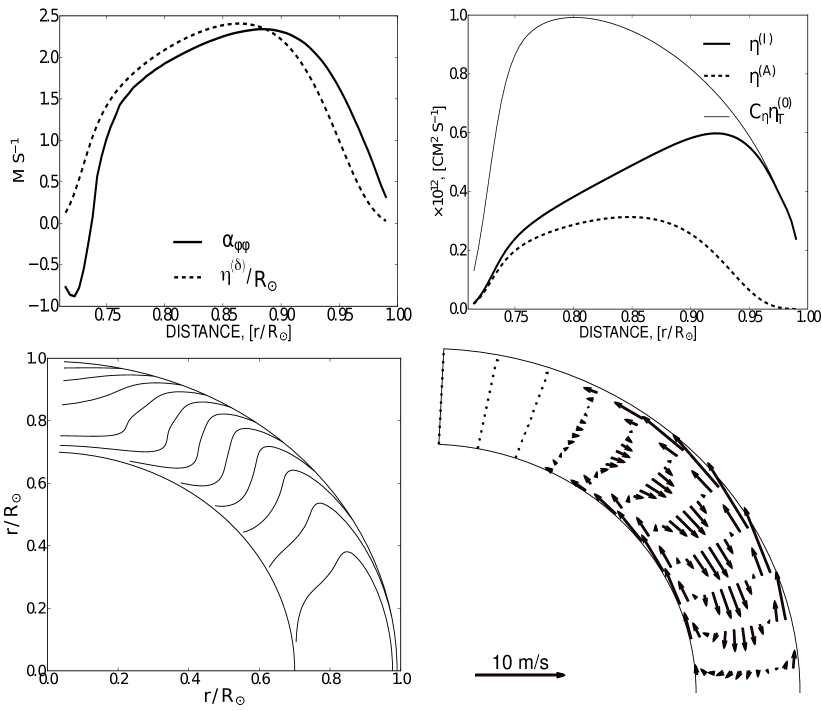
Figure 1: Panel (a), the radial profiles of components of the helicity coefficient, $\alpha$, (Eq.10) and the $\Omega\times J$ term (Eq. 15) for $\theta=45^{\circ}$, the $\Omega\times J$ effect was normalized by $R_{\odot}$ and amplified by factor 10 to show at the same amplitude range as the $\alpha$ effect; panel (b), the radial profiles of the background turbulent diffusivity $C_{\eta}\eta_{T}^{(0)}$, the isotropic, $\eta^{(I)}$, and anisotropic, $\eta^{(A)}$, parts of the magnetic diffusivity coefficients;c) the angular velocity distribution; (d) velocity vectors of the double-cell meridional circulation pattern .

For axisymmetric large-scale magnetic fields the vector-potential can be represented as a sum of the azimuthal and poloidal components (Krause & Rädler, 1980):

$$\overline{\mathbf{A}}=\mathbf{e}_{\phi}T+\mathbf{r}P=\frac{\mathbf{e}_{\phi}}{r\sin\theta}A+r\mathbf{e}_{r}P.$$ (6)

The toroidal part of the vector potential, $A$, is governed by the dynamo equations (Eq.1). The poloidal part of the vector potential, $P$, can be found from the toroidal magnetic field component, $B$, using equation $\boldsymbol{\nabla}\times\left(\mathbf{r}P\right)=\mathbf{e}_{\phi}B$. The reconstruction is simple by using pseudo-spectral numerical schemes which are based on the Legendre polynomial decomposition for the latitudinal profile of $B$. Following Pipin & Kosovichev (2011c) we use a combination of the “open” and “closed” boundary conditions at the top, controlled by a parameter $\delta=0.99$:

$$\delta\frac{\eta_{T}}{r_{e}}B+\left(1-\delta\right)\mathcal{E}_{\theta}=0.$$ (7)

This is similar to the boundary condition discussed by Kitchatinov et al. (2000). For the poloidal field we apply a combination of the local condition $A=0$ and condition of smooth transition from the internal poloidal field to the external potential (vacuum) field:

$$\delta\left(\left.\frac{\partial A}{\partial r}\right|_{r=r_{e}}-\left.\frac{\partial A^{(vac)}}{\partial r}\right|_{r=r_{e}}\right)+\left(1-\delta\right)A=0,$$ (8)

For the magnetic helicity we employ $\bar{\chi}=0$ at the bottom of the convection zone, and we assume that the radial derivative of the total helicity is zero at the top. The initial magnetic field is assumed dipolar with a small quadrupolar component to check the parity preference when the solution reaches a stationary state.

3 Results and discussion

Figure 2 shows the snapshots of the magnetic field and magnetic helicity evolution in the North segment of the solar convection zone for the model with the circulation speed $U_{0}=12$m/s. The similar snapshots for the model without circulation can be found in (Pipin et al., 2013). We observe drift of the dynamo waves related to the evolution of the large-scale toroidal and poloidal fields, towards the equator and towards the pole, respectively. It is found that the meridional circulation accelerates the equator-ward drift of the toroidal magnetic field near the surface and the poleward drift of the toroidal magnetic field near the bottom of the convection zone.

The snapshots on Figure 2 illustrate the evolution of the large-scale magnetic fields (Fig.2a) and magnetic helicity (Fig.2b). The toroidal magnetic field of the new cycle is generated near the bottom of the convection zone by the differential rotation. Simultaneously, we see a start of generation of the poloidal magnetic field (contour lines) by the $\alpha$- and $\Omega\times J$ effects. The dynamo wave propagates by the turbulent diffusion processes almost radially to the surface following the Parker-Yoshimura rule (Parker, 1955; Yoshimura, 1975). However, the propagation of the wave is inclined to the equator because of the anisotropy of the turbulent diffusion and turbulent transport effects (Kitchatinov, 2002). Near the surface the turbulent downward pumping and the subsurface rotational shear (Pipin & Kosovichev, 2011b) stop the radial propagation and deflect the dynamo wave toward the equator. The near-surface meridional circulation and the turbulent diffusion bring the decaying poloidal field to the poles.

The meridional circulation modifies the propagation of the dynamo wave. It is found that the toroidal magnetic field is strongly involved in clockwise advection by the bottom circulation cell in a manner which is typical for the flux transport models. The inner part of the poloidal magnetic field flux is carried by the meridional flow in a similar way. Near the surface the poloidal field migrates towards the poles at high latitudes and towards the equator at low latitudes.

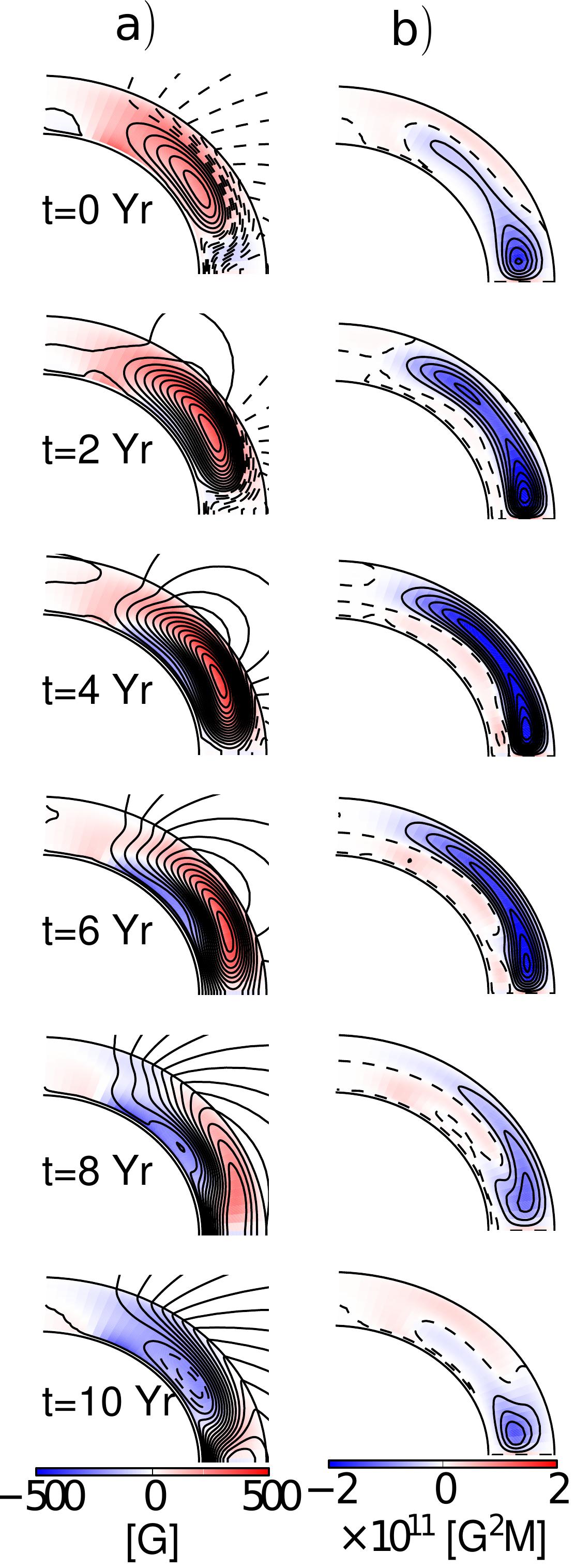
Figure 2: a) Evolution of the large-scale magnetic field inside the convection zone for the dynamo model with the meridional circulation speed $U_{0}=12$ m/s. The field lines show of the poloidal component of the mean magnetic field, and the toroidal magnetic field (varies $\pm 0.6$kG) is shown by the background images. b) Evolution of the large-scale magnetic helicity density (contours) and the mean helicity density of small-scale fields (background images). Both parts of the helicity density vary within the same range of magnitudes.

Figure 2b shows the evolution of large-scale (contours) and small-scale (colors) magnetic helicities. As suggested by the helicity conservation law (Eq. 4), the evolution of the mean helicity density of small-scale fields follows the evolution of the helicity density of large-scale magnetic fields. In the upper part of the convection zone the small-scale magnetic helicity obeys the so-called helicity hemispheric sign rule (hereafter “magnetic helicity sign rule”) (Seehafer, 1994): it is negative sign in the Northern hemisphere and positive in the Southern hemisphere. The reversals of the helicity hemispheric rule can be found at high latitudes at the beginning of the cycle when the large-scale magnetic helicity is determined by the contribution of the near surface poloidal magnetic field (cf snapshots for the $t=2$yr). The reversals of the magnetic helicity sign rule have the different origin in the flux-transport and mean-field dynamo models (see, e.g, Choudhuri et al., 2004; Zhang et al., 2012; Pipin, 2013; Pipin et al., 2013).

Figure 3 shows the time-latitude “butterfly” diagrams of the toroidal (contours) and radial (colors) magnetic fields evolution in the upper part of the solar convection zone for the meridional flow speed $U_{0}=0$, 12 and 20 m/s. In all cases (with and without the circulation) there is the qualitative agreement with observations. We found that the maximum of the toroidal magnetic field migrates closer to the equator for the models which include the circulation. However, in these cases the butterfly diagram wings are wider in latitude than in the case without circulation. Also it is found that the circulation reduces the latitudinal width of the polar branch for the radial magnetic field evolution and also reduces the overlap between the cycles. We draw these diagrams only for one hemisphere because in all these cases the antisymmetric mode (dipole-like) is dominant.

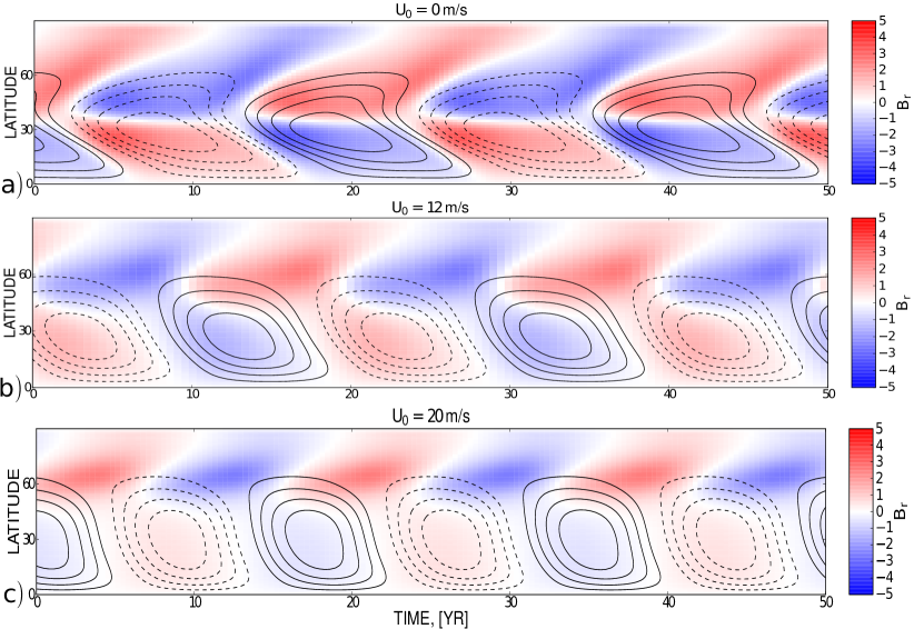
Figure 3: (a) the time - latitude variations (“butterfly diagrams”) for the model without meridional circulation; (b) the same for the model with the meridional circulation of $U_{0}=12$ m/s; (c) the same as (b) for $U_{0}=20$ m/s. The toroidal field near the surface, at $r=0.92R_{\odot}$, is shown by contours (plotted for $\pm 100$G range), and the surface radial magnetic field is shown by background red-blue images.

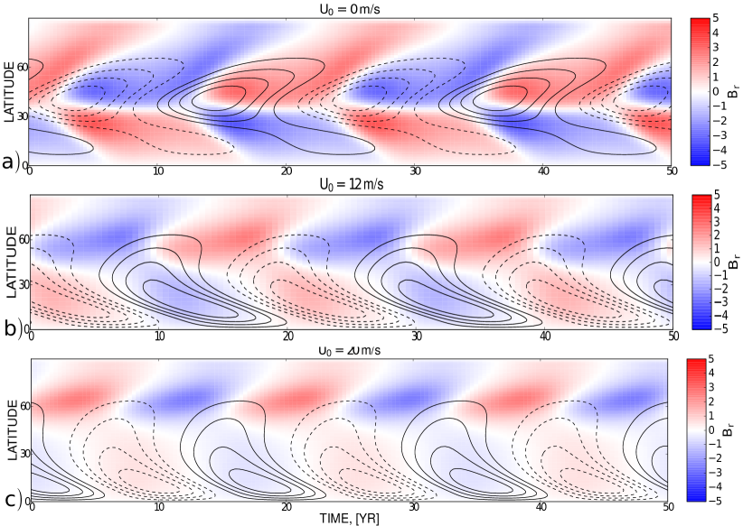
Figure 4: The same as Figure 3 for the toroidal magnetic field (contour lines) at $r=0.82R_{\odot}$.

Figure 4 shows the toroidal magnetic field evolution in the middle part of the solar convection zone where the flows of the two cells converge. In the model without circulation the polar branch of the toroidal magnetic field is dominant. When the amplitude of the circulation speed is greater than $U_{0}=8$m/s the toroidal magnetic field is swept towards the equator. In this case the time-latitude patterns of the toroidal magnetic field evolution in the middle of the convection zone are very similar to those suggested by the standard flux-transport and advection dominated dynamos (Bonanno et al., 2002; Rempel, 2006; Jouve & Brun, 2007) near the bottom of the convection zone.

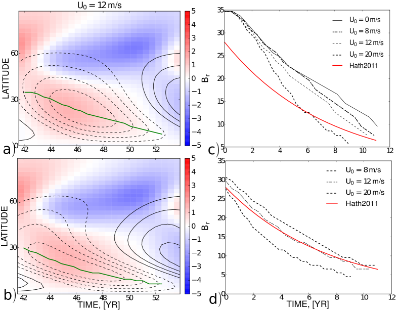
Figure 5: To calculation of the latitudinal coordinates of the maximum of the toroidal magnetic field flux. Panels a) and b) show the examples of the time-latitude pattern of the magnetic field evolution at $r=0.92R_{\odot}$(a) and $0.82R_{\odot}$(b) for the model with $U_{0}=12$m/s. The toroidal field is shown by contours, and the radial field is shown by background images. The green solid line shows position of the toroidal magnetic field flux maxima. Panels c) and d) show the results of calculations for the different models at $r=0.92R_{\odot}$(c) and $0.82R_{\odot}$(d) . Red line marks the observational results by Hathaway (2011).

To compare the butterfly diagram shapes with solar observations we calculate the latitudinal coordinates of the maximum of the toroidal magnetic field flux. The results for the magnetic flux that resides at two depths ($r=0.92R_{\odot}$ and $r=0.82R_{\odot}$) in the solar convection zone are shown in the Figure 5. The observations, (see e.g., Hathaway, 2011) suggest that the latitude of the maximum of the sunspot formation decreases exponentially in course of the solar cycle. The model with $U_{0}=12$m/s is in the best agreement with the observations if the sunspot flux originates at $r=0.82R_{\odot}$. In the model, which does not include circulation the toroidal magnetic field flux does not approach the equator as close as in the model with circulations, which show somewhat better agreement with the observations. However their qualitative behaviors are similar.

Figure 6: Dependences of the maximum of the toroidal magnetic field strength in the convection zone, the dynamo period and the magnitude of the axial dipole on the amplitude of the meridional circulation speed, $U_{0}$.

Figure 6 shows the dependence of maximum of the toroidal magnetic field strength inside the solar convection zone, the dynamo period and the magnitude of the axial magnetic dipole on the amplitude of the meridional circulation $U_{0}$. All parameters were computed for the same dynamo parameter $C_{\alpha}$. The amplitude of the generated magnetic field as well as the dynamo period decrease monotonically with the increase of the circulation speed. However, there is a plateau in the range of $U_{0}$ between 8m/s and 14m/s. Interesting that the magnitude of the generated axial dipole varies substantially within the same range. The growth of the magnetic dipole corresponds to the enhanced poloidal magnetic field generation in this interval of the circulation speed, which can be due to a resonance between the meridional circulation and the dynamo wave propagation in the middle of the convection zone. This suggestion requires further detailed studies.

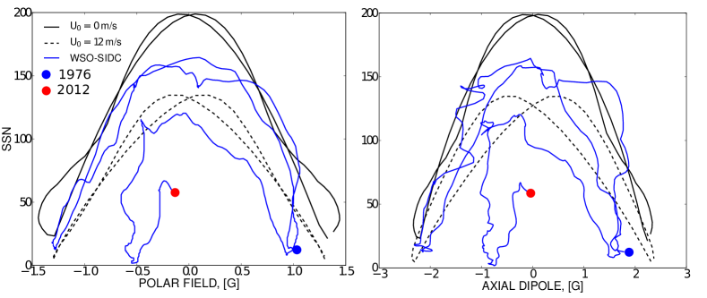
Figure 7: The phase relations between a) the strength of the polar magnetic field and the sunspot number and b) the axial dipole and the sunspot number in our models (black curves) and in the observations (noisy blue curves).

The interesting question is how the circulation changes the phase relation between the polar magnetic field strength and the sunspot activity in our model. The simulated sunspot number (SSN) was computed following Pipin et al. (2012), as $\textnormal{SSN}={\displaystyle B_{max}\exp\left(-\frac{B_{0}}{B_{max}}\right)}$, where $B_{0}=600$G and $B_{max}$ is the maximum of the toroidal magnetic field strength at $r=0.92R_{\odot}$. The results are shown in Figure 7. To compare with observations we used the smoothed sunspot number provided by SIDC (SIDC, 2010). The observations of the Wilcox Solar Observatory (Svalgaard et al., 1978; Hoeksema, 1995) provide us with the strength of the line-of-sight polar magnetic field which was averaged over the polemost $3^{\prime}$ aperture. The magnitude of the axial dipole was computed from the coefficients of the potential extrapolation of the surface magnetic field. In the model we will assume that the measured signal of the line-of-sight component of the field is formed by the radial component of the large-scale magnetic field. The strength of the axial dipole in the model is calculated from the first coefficient of the vector-potential expansion at the top boundary. Figure 7 illustrates the phase relations between the sunspot number and the polar radial magnetic field in the models and in observations. In the phase digrams the maxima of the polar magnetic field and the axial dipole correspond to the minima of the sunspot number. The reversals of the polar magnetic field correspond to the sunspot maxima. For the axial dipole this phase relation fluctuates and observations show a delay of about two years in the last solar cycle, which is not explained in our models.

In the case of ideal synchronization the two subsequent cycles would produce the parabolic curve in the phase diagrams. This is also found for the sunspot Cycles 21 and 22 which were not very different in amplitude. Cycle 23 had a smaller magnitude, and started with the polar magnetic field of about 1 G in the minimum as the previous two cycles. While our model qualitatively reproduces the phase relation, it does not explain observed a sudden decrease of the sunspot activity in Cycle 23.

In these calculations, we assumed that the sunspot activity originates from the toroidal magnetic field at $r=0.92R_{\odot}$ ( just below the subsurface shear layer) because this depth provided the best agreement with observations for the model without circulation flow. It is interesting that for the models with the meridional flow the acceptable range of the depths is significantly broader.

We investigated the stability of the obtained solutions with respect to changes of the circulation pattern and the other parameters of the model. The results similar shown in Figures 2 and 3, are obtained for the case of pure a $\alpha^{2}\Omega$ dynamo (without the $\Omega\times J$ effect). However, in this case, the cycle overlap in the time-latitude diagrams is much stronger than in Figures 3(b,c). The similar time-latitude butterfly diagrams are obtained also for the case when the meridional circulation forms only one cell per hemisphere with the stagnation point radius larger than $0.85R$. This is because of the subsurface rotational shear layer, which plays the primary role in the model. For the deeper stagnation point the dynamo wave is dominated by the toroidal magnetic field near the bottom of the convection zone (Pipin & Kosovichev, 2011a). Also, we checked the effect of the meridional circulation in the simplified model which was presented by Pipin & Kosovichev (2011c). In that model the $\alpha$-effect was confined in the low-latitude $\pm 30^{\circ}$ zone. The results are generally similar to what is shown in Figures 2 and 3.

4 Conclusions

The main findings can be summarized as follows. The mean-field dynamo model that includes the subsurface rotational shear layer and the double-cell (in radius) meridional circulation, indicated by the recent helioseismology results, can reproduce the solar magnetic cycles in the form of the time-latitude “butterfly” diagrams. The double-cell circulation affects the distribution of the magnetic field with radius in the convection zone, increasing the field concentration to the convection zone boundaries, and n the middle of the convection zone where the two cells converge. The latter effect can lead to a non-monotonic profile of the amplitude of the large-scale poloidal magnetic field in response to an increase of the circulation speed. The models qualitatively explains the observed synchronization between the polar magnetic field strength and the sunspot number. However, it does not explain the sudden drop of the Sun’s magnetic activity in Cycle 23. This question has to be examined further in order to clarify the detail of this synchronization. By comparing the toroidal field migration speed at the different depths with the observed characteristics speed of the sunspot formation zone we found that the range of the depth of the active region emerging flux can be between 0.82-0.92$R_{\odot}$. This estimate can be improved for a more precise helioseismology measurements of the meridional circulation.

5 Appendix

Here, we give some details about calculations of the mean electromotive force. The more elaborated description can be found in one of our previous papers (e.g., Pipin & Kosovichev, 2011b). The mean electromotive force is given as follows (Pipin, 2008).

$$\mathcal{E}_{i}=\left(\alpha_{ij}+\gamma_{ij}^{(\Lambda)}\right)\overline{B}_{j}-\left(\eta_{ijk}+\eta_{ijk}^{(\delta)}\right)\nabla_{j}\overline{B}_{k}.$$ (9)

The tensor $\alpha_{ij}$, representing the so-called $\alpha$-effect, includes hydrodynamic ($\alpha_{ij}^{(H)}$) and magnetic ($\alpha_{ij}^{(M)}$) helicity contributions:

$$\alpha_{ij} = C_{\alpha}\psi_{\alpha}\sin^{2}\theta\alpha_{ij}^{(H)}+\alpha_{ij}^{(M)},$$ (10)

$$\alpha_{ij}^{(H)} = 3\eta_{T}\frac{\delta_{ij}}{\Omega}\left\{\left(f_{10}^{(a)}\left(\boldsymbol{\mathbf{\Omega}}\cdot\boldsymbol{\Lambda}^{(\rho)}\right)+f_{11}^{(a)}\left(\boldsymbol{\mathbf{\Omega}}\cdot\boldsymbol{\Lambda}^{(u)}\right)\right)\right\}$$

$$+ 3\eta_{T}\frac{\Omega_{i}\Omega_{j}}{\Omega^{3}}\left\{\left(f_{5}^{(a)}\left(\boldsymbol{\mathbf{\Omega}}\cdot\boldsymbol{\Lambda}^{(\rho)}\right)+f_{4}^{(a)}\left(\boldsymbol{\mathbf{\Omega}}\cdot\boldsymbol{\Lambda}^{(u)}\right)\right)\right\}$$

$$+ \frac{3\eta_{T}}{\Omega}\left\{\left(\Omega_{i}\Lambda_{j}^{(\rho)}+\Omega_{j}\Lambda_{i}^{(\rho)}\right)f_{6}^{(a)}+\left(\Omega_{i}\Lambda_{j}^{(u)}+\Omega_{j}\Lambda_{i}^{(u)}\right)f_{8}^{(a)}\right\},$$ (12)

where $\mathbf{\Lambda}^{(\rho)}=\boldsymbol{\nabla}\log\overline{\rho}$ quantifies the density stratification (inverse density scale height), $\mathbf{\Lambda}^{(u)}=\frac{1}{2}\boldsymbol{\nabla}\log\left(\eta_{T}^{(0)}\right)$ quantifies the stratification of turbulent diffusivity $\eta_{T}^{(0)}$. The $\alpha$-quenching function $\psi_{\alpha}=-3/4\phi_{6}^{(a)}\left(\beta\right)$ depends on $\beta={\displaystyle\left|\overline{B}\right|/\sqrt{\overline{\rho}\mu_{0}\overline{u^{2}}}}$, and $\phi_{6}^{(a)}$ is given in P08.

The turbulent pumping coefficient, $\gamma_{ij}^{(\Lambda)}$, depends on the mean density and turbulent diffusivity stratification, and also on the Coriolis number $\Omega^{*}=2\tau_{c}\Omega_{0}$, where $\tau_{c}$ is a typical convective turnover time, and $\Omega_{0}$ is the angular velocity. Following the results of P08, $\gamma_{ij}^{(\Lambda)}$ is expressed as follows:

$$\gamma_{ij}^{(\Lambda)} = 3\eta_{T}\left\{f_{3}^{(a)}\Lambda_{n}^{(\rho)}+f_{1}^{(a)}\left(\boldsymbol{\Omega}\cdot\boldsymbol{\Lambda}^{(\rho)}\right)\frac{\Omega_{n}}{\Omega}\right\}\varepsilon_{inj}-3\eta_{T}f_{1}^{(a)}\frac{\Omega_{j}}{\Omega^{2}}\varepsilon_{inm}\Omega_{n}\Lambda_{m}^{(\rho)},$$

$$- 3\eta_{T}\left(\varepsilon-1\right)\left\{f_{2}^{(a)}\Lambda_{n}^{(u)}+f_{1}^{(a)}\frac{\left(\boldsymbol{\Omega}\cdot\boldsymbol{\Lambda}^{(u)}\right)}{\Omega^{2}}\Omega_{n}\right\}\varepsilon_{inj}.$$

The turbulent diffusivity is anisotropic due to the Coriolis force, and is given by:

$$\eta_{ijk}=3\eta_{T}\left\{\left(2f_{1}^{(a)}-f_{2}^{(d)}\right)\varepsilon_{ijk}-2f_{1}^{(a)}\frac{\Omega_{i}\Omega_{n}}{\Omega^{2}}\varepsilon_{njk}\right\}.$$ (14)

We also include the nonlinear effects of magnetic field generation induced by the large-scale current and global rotation, which are usually called the $\Omega\times J$-effect or the $\delta$ dynamo effect (Rädler, 1969). Their importance is supported by the numerical simulations (Käpylä et al., 2008; Schrinner, 2011). We use the equation for $\eta_{ijk}^{(\delta)}$ which was suggested in P08 (also, see, Rogachevskii & Kleeorin, 2004):

$$\eta_{ijk}^{(\delta)}=3\eta_{T}C_{\delta}f_{4}^{(d)}\frac{\Omega_{j}}{\Omega}\left\{\tilde{\varphi}_{7}^{(w)}\delta_{ik}+\tilde{\varphi}_{2}^{(w)}\frac{\overline{B}_{i}\overline{B}_{k}}{\overline{B}^{2}}\right\},$$ (15)

where, $C_{\delta}$ measures the strength of the $\Omega\times J$ effect, $\tilde{\varphi}_{2,7}^{(w)}\left(\beta\right)$ are normalized versions of the magnetic quenching functions $\varphi_{2,7}^{(w)}$ given in P08. They are defined as follows, $\tilde{\varphi}_{2,7}^{(w)}\left(\beta\right)=\frac{5}{3}\varphi_{2,7}^{(w)}\left(\beta\right)$. The functions $f_{\{1-11\}}^{(a,d)}$in Eqs (10,5,14, 15) depend on the Coriolis number. They can be found in P08, as well.

References

- Bonanno et al. (2006) Bonanno, A., Elstner, D., Belvedere, G., & Rüdiger, G. 2006, Memorie della Societa Astronomica Italiana Supplementi, 9, 71
- Bonanno et al. (2002) Bonanno, A., Elstner, D., Rüdiger, G., & Belvedere, G. 2002, A&A, 390, 673
- Brandenburg (2005) Brandenburg, A. 2005, ApJ, 625, 539
- Brandenburg et al. (2012) Brandenburg, A., Rädler, K.-H., & Kemel, K. 2012, A&A, 539, A35
- Brown et al. (2011) Brown, B. P., Browning, M. K., Brun, A. S., Miesch, M. S., & Toomre, J. 2011, in Astronomical Society of the Pacific Conference Series, Vol. 448, 16th Cambridge Workshop on Cool Stars, Stellar Systems, and the Sun, ed. C. Johns-Krull, M. K. Browning, & A. A. West, 277
- Charbonneau (2011) Charbonneau, P. 2011, Living Reviews in Solar Physics, 2, 2
- Choudhuri et al. (2004) Choudhuri, A. R., Chatterjee, P., & Nandy, D. 2004, ApJ, 615, L57
- Dikpati & Charbonneau (1999) Dikpati, M., & Charbonneau, P. 1999, ApJ, 518, 508
- Guerrero et al. (2013) Guerrero, G., Smolarkiewicz, P. K., Kosovichev, A., & Mansour, N. 2013, in Solar and Astrophysical Dynamos and Magnetic Activity, IAUS 294
- Hathaway (2011) Hathaway, D. H. 2011, Sol. Phys., 273, 221
- Hoeksema (1995) Hoeksema, J. T. 1995, Space Sci. Rev., 72, 137
- Howe et al. (2011) Howe, R., Larson, T. P., Schou, J., Hill, F., Komm, R., Christensen-Dalsgaard, J., & Thompson, M. J. 2011, Journal of Physics Conference Series, 271, 012061
- Hubbard & Brandenburg (2012) Hubbard, A., & Brandenburg, A. 2012, ApJ, 748, 51
- Jouve & Brun (2007) Jouve, L., & Brun, A. S. 2007, A&A, 474, 239
- Käpylä et al. (2008) Käpylä, P. J., Korpi, M. J., & Brandenburg, A. 2008, A&A, 491, 353
- Käpylä et al. (2009) —. 2009, A&A, 500, 633
- Käpylä et al. (2012) Käpylä, P. J., Mantere, M. J., & Brandenburg, A. 2012, ApJ, 755, L22
- Kitchatinov (2002) Kitchatinov, L. L. 2002, A&A, 394, 1135
- Kitchatinov (2011) Kitchatinov, L. L. 2011, in Astronomical Society of India Conference Series, Vol. 2, Astronomical Society of India Conference Series, 71–80
- Kitchatinov et al. (2000) Kitchatinov, L. L., Mazur, M. V., & Jardine, M. 2000, A&A, 359, 531
- Kleeorin & Rogachevskii (2003) Kleeorin, N., & Rogachevskii, I. 2003, Phys. Rev. E, 67, 026321
- Krause & Rädler (1980) Krause, F., & Rädler, K.-H. 1980, Mean-Field Magnetohydrodynamics and Dynamo Theory (Berlin: Akademie-Verlag), 271
- Miesch et al. (2011) Miesch, M. S., Brown, B. P., Browning, M. K., Brun, A. S., & Toomre, J. 2011, in IAU Symposium, Vol. 271, IAU Symposium, ed. N. H. Brummell, A. S. Brun, M. S. Miesch, & Y. Ponty, 261–269
- Miesch et al. (2006) Miesch, M. S., Brun, A. S., & Toomre, J. 2006, ApJ, 641, 618
- Mitra et al. (2010) Mitra, D., Candelaresi, S., Chatterjee, P., Tavakol, R., & Brandenburg, A. 2010, Astronomische Nachrichten, 331, 130
- Mitra-Kraev & Thompson (2007) Mitra-Kraev, U., & Thompson, M. J. 2007, Astronomische Nachrichten, 328, 1009
- Ossendrijver et al. (2001) Ossendrijver, M., Stix, M., & Brandenburg, A. 2001, A&A, 376, 713
- Ossendrijver et al. (2002) Ossendrijver, M., Stix, M., Brandenburg, A., & Rüdiger, G. 2002, A&A, 394, 735
- Parker (1955) Parker, E. N. 1955, ApJ, 121, 491
- Pipin (2008) Pipin, V. V. 2008, Geophysical and Astrophysical Fluid Dynamics, 102, 21
- Pipin (2013) Pipin, V. V. 2013, in Solar and Astrophysical Dynamos and Magnetic Activity Proceedings IAU Symposium No. 294
- Pipin & Kosovichev (2011a) Pipin, V. V., & Kosovichev, A. G. 2011a, ApJ, 738, 104
- Pipin & Kosovichev (2011b) —. 2011b, ApJ, 741, 1
- Pipin & Kosovichev (2011c) —. 2011c, ApJL, 727, L45
- Pipin et al. (2012) Pipin, V. V., Sokoloff, D. D., & Usoskin, I. G. 2012, A&A, 542, A26
- Pipin et al. (2013) Pipin, V. V., Sokoloff, D. D., Zhang, H., & Kuzanyan, K. M. 2013, ApJ, 768, 46
- Rädler (1969) Rädler, K.-H. 1969, Monats. Dt. Akad. Wiss., 11, 194
- Rempel (2006) Rempel, M. 2006, ApJ, 647, 662
- Rogachevskii & Kleeorin (2004) Rogachevskii, I., & Kleeorin, N. 2004, ArXiv Astrophysics e-prints
- Rogachevskii et al. (2011) Rogachevskii, I., Kleeorin, N., Käpylä, P. J., & Brandenburg, A. 2011, Phys. Rev. E, 84, 056314
- Ruediger & Brandenburg (1995) Ruediger, G., & Brandenburg, A. 1995, A&A, 296, 557
- Schrinner (2011) Schrinner, M. 2011, A&A, 533, A108
- Seehafer (1994) Seehafer, N. 1994, A&A, 284, 593
- SIDC (2010) SIDC. 2010, Monthly Report on the International Sunspot Number, online catalogue, http://www.sidc.be/sunspot-data/
- Stix (2002) Stix, M. 2002, The sun: an introduction, 2nd edn. (Berlin : Springer), 521
- Svalgaard et al. (1978) Svalgaard, L., Duvall, Jr., T. L., & Scherrer, P. H. 1978, Sol. Phys., 58, 225
- Yoshimura (1975) Yoshimura, H. 1975, ApJ, 201, 740
- Zhang et al. (2012) Zhang, H., Moss, D., Kleeorin, N., Kuzanyan, K., Rogachevskii, I., Sokoloff, D., Gao, Y., & Xu, H. 2012, ApJ, 751, 47
- Zhao et al. (2012) Zhao, J., Bogart, R. S., Kosovichev, A. G., & Duvall, Jr., T. L. 2012, in American Astronomical Society Meeting Abstracts, Vol. 220, American Astronomical Society Meeting Abstracts #220, 109.05