Non-stationary subdivision schemes originated from uniform trigonometric B-spline

Abstract

The paper proposes, an algorithm to produce novel $m$-point (for any integer $m\geq 2$) binary non-stationary subdivision scheme. It has been developed using uniform trigonometric B-spline basis functions and smoothness is being analyzed using the theory of asymptotically equivalence. The results show that the most of well-known binary approximating schemes can be considered as the non-stationary counterpart of the proposed algorithm.

Furthermore, the schemes developed by the proposed algorithm has the ability to reproduce or regenerate the conic sections, trigonometric polynomials and trigonometric splines as well. Some examples are considered, by choosing an appropriate tension parameter $0<\alpha<\pi/3$, to show the usefulness.

1 Introduction

Subdivision scheme is one of the most important and significant modelling tool to create smooth curves from initial control polygon by subdividing them according to some refining rules, recursively. These refining rules take the initial polygon to produce a sequence of finer polygons converging to a smooth limiting curve.

In the field of non-stationary subdivision schemes, Beccari et al. [1] presented a 4-point binary non-stationary interpolating subdivision scheme, using tension parameter, that was capable of producing certain families of conics and cubic polynomials. They also developed a 4-point ternary interpolating non-stationary subdivision scheme in the same year that generate $C^{2}$ continuous limit curves showing considerable variation of shapes with a tension parameter [2]. A new family of 6-point interpolatory non-stationary subdivision scheme was introduced by Conti and Romani [4]. It was presented using cubic exponential B-spline symbol generating functions that can reproduce conic sections. Conti and Romani [5] discussed algebraic conditions on non-stationary subdivision symbols for exponential polynomial reproduction.

Since, non-stationary schemes have proven to be efficient iterative algorithms to construct special classes of curves. One of the important capability is the reproduction or regeneration of trigonometric polynomials, trigonometric splines and conic sections, in particular circles, ellipses etc. So, in this article, an algorithm has been introduced to produce $m-$point binary approximating non-stationary schemes, for any integer $m\geq 2$, using the uniform trigonometric B-spline basis function of order $m-1$. The proposed algorithm can be considered as the non-stationary counterpart of the well known binary approximating schemes introduced by Chakin [3] and Siddiqi with his different co-authors [9, 13, 14, 15, 16], after setting different values of $m$ in proposed algorithm (for details see table 5.1). Moreover, the proposed algorithm can also be considered as generalization form of the 2-point and 3-point non-stationary schemes presented by Daniel and Shunmugaraj [6].

The paper is organized as follows, in section $2$ the basic notion and definitions of binary subdivision scheme are considered. The algorithm, to produce $m-$point binary non-stationary scheme, is presented in section $3$. Some example are considered, to construct the masks of 2-point, 3-point and 4-point schemes, in section 4. The convergence and smoothness of the schemes are being calculated in section $5$. Some properties and advantages of proposed algorithm are being discussed in section $6$. The conclusion is drawn in section $7$.

2 Preliminaries

In univariate subdivision scheme, following the notion and definitions introduced in [10], the set of control points $\{f_{i}^{k}\in R\mid i\in Z\}$ of polygon at $k^{th}$ level is mapped to a refined polygon to generate the new set of control points $\{f_{i}^{k+1}\in R\mid i\in Z\}$ at the $(k+1)^{st}$ level by applying the following repeated application of the refinement rule

$$f^{k+1}_{i}=\{S_{a^{(k)}}f^{k}\}_{i}=\sum_{j\in Z}a^{(k)}_{i-2j}f^{k}_{j} \forall~{}i\in Z,$$ ( 2. 1 )

with the sequence of finite sets of real coefficients $\{a_{i}^{(k)},k\geq 0\}$ constitute the so-called mask of subdivision scheme. If the mask of a scheme are independent of $k$, namely if $a^{(k)}=a$ for all $k\geq 0$ then it is called stationary $S_{a}$, otherwise it is called non-stationary $S_{a^{(k)}}$.

The convergent subdivision scheme, formally denoted by $f^{k+1}=S_{a^{(k)}}f^{k}$, with the corresponding mask $a_{i}^{(k)}~{}i\in Z$ necessarily satisfies

$$\sum_{j\in Z}a^{(k)}_{2j}\cong\sum_{j\in Z}a^{(k)}_{2j+1}\cong 1.$$

A binary non-stationary subdivision scheme $S_{a^{(k)}}$ is said to be convergent if for every initial data $f^{0}\in l^{\infty}$ there exits a continuous limit function $g\in C^{m}(R)$ such that

$$\lim_{k\rightarrow\infty}\sup_{i\in Z}|f_{i}^{k}-g(2^{-k}i)|=0,$$

and $g$ is not identically zero for some initial data $f^{0}$.

We also recall that two univariate binary schemes $S_{a^{(k)}}$ and $S_{b^{(k)}}$ are said to be asymptotically equivalent if

$$\sum^{\infty}_{k=1}\|S_{a^{(k)}}-S_{b^{(k)}}\|_{\infty}<\infty,$$

where

$$\|S_{a^{(k)}}\|_{\infty}=max\{\sum_{i\in Z}|a_{2i}^{(k)}|,\sum_{i\in Z}|a_{2i+1}^{(k)}|\}$$

Theorem 2.1. The non-stationary scheme $S_{a^{(k)}}$ and stationary scheme $S_{a}$ are said to be asymptotically equivalent schemes, if they have finite masks of the same support. The stationary scheme $S_{a}$ is $C^{m}$ and

$$\sum^{\infty}_{k=0}2^{mk}\|S_{a^{(k)}}-S_{a}\|_{\infty}<\infty,$$

then non-stationary scheme $S_{a^{(k)}}$ is also said to be $C^{m}$.

3 The algorithm for approximating schemes

In this section, an algorithm has been introduced to produce $m$-point binary non-stationary subdivision schemes (for any integer $m\geq 2$) which can generate the families of $C^{m-1}$ limiting curves by choosing a tension parameter $0<\alpha<\pi/3$. The algorithm has been established using uniform trigonometric B-splines of order n. So, in view of Koch et al. [11], trigonometric B-splines can be defined as follow. Let $m>n>0$ and $0<\alpha<\frac{\pi}{n}$, then Uniform Trigonometric B-splines $\{T_{j}^{n}(x;\alpha)\}_{j=1}^{m}$ of order $n$ associated with the knot sequence $\Delta:=\{t_{i}=i\alpha:i=0,1,2,...,m+n\}$ with the mesh size $\alpha$ are defined by the recurrence relation,

$$T^{1}_{0}(x;\alpha)=\left\{\begin{array}[]{rr}1,&x\in[0,\alpha)\\ 0,&otherwise,\\ \end{array}\right.$$

for $1<r\leq n,$

$$T^{r}_{0}(x;\alpha)=\frac{1}{\sin((r-1)\alpha)}\{\sin(x)T_{0}^{r-1}(x;\alpha)+\sin(t_{r}-x)T_{0}^{r-1}(x-\alpha;\alpha)\}$$ ( 3. 3 )

and $T^{r}_{j}(x;\alpha)=T^{r}_{0}(x-j\alpha;\alpha),$ for $j=1,2,...,m$. The trigonometric B-spline $T^{n}_{j}(x;\alpha)$ is supported on $[t_{j},t_{j+n}]$ and it is the interior of its support. Moreover, $\{T^{n}_{j}\}_{j=1}^{m}$ are linearly independent set on the interval $[t_{n-1},t_{m+1}]$. Hence, on this interval, any uniform trigonometric spline $S(x)$ has a unique representation of the form $S(x)=\sum_{j=0}^{m}p_{j}T_{j}^{n}(x;\alpha),~{}~{}p_{j}\in R$.

To obtain the mask $a_{i}^{k}(\alpha)=a_{i}^{k},~{}~{}i=0,1,2,...,m-1$ we use the following recreance relation, for any value of $k$,

$$a_{i}^{k}(\alpha)=T_{0}^{m}\left((m-i-1)\frac{\alpha}{2^{k}}+\frac{\alpha}{2^{k+2}};\frac{\alpha}{2^{k}}\right)~{}~{}~{}~{}~{}i=0,1,2,...,m-1$$ ( 3. 4 )

where $T_{0}^{m}\left(x;\frac{\alpha}{2^{k}}\right)$, with mesh size $(\frac{\alpha}{2^{k}})$, is a trigonometric B-spline basis function of order $m-1$ and can be calculated form equation (3.2). It can also be observed that the schemes produced by the proposed algorithm do not have the convex hull and affine invariance properties. Since the sums of the weights of the obtained schemes at $kth$ level are not equal to unity. To get sum of the mask equal to unity, the corresponding normalized scheme can be obtained (see [6]). In the following, some examples are considered to produce the masks of 2-point, 3-point and 4-point binary approximating schemes after setting $m=2$, 3 and 4, respectively, in above recurrence relation.

4 Construction of the schemes

In this section, some applications are considered to construct the masks of 2-point, 3-point and 4-point approximating non-stationary schemes.

4.1 The 2-point Approximating Scheme

The linear trigonometric B-spline basis function $T_{0}^{2}\left(x;\frac{\alpha}{2^{k}}\right)$, with mesh size $(\frac{\alpha}{2^{k}})$, can be calculated by setting $m=2$ in relation (3.3). The 2-point binary non-stationary scheme (which is also called corner cutting scheme) with mask $a_{i}^{(k)}(\alpha)=a_{i}^{(k)},i=0,1$ is defined, for any value of $k$ and $\alpha\in]0,\frac{\pi}{3}[$, as

$$\left.\begin{array}[]{rrr}f^{k+1}_{2i}&=&a_{0}^{(k)}f^{k}_{i}+a_{1}^{(k)}f^{k}_{i+1}\\ f^{k+1}_{2i+1}&=&a_{1}^{(k)}f^{k}_{i}+a_{0}^{(k)}f^{k}_{i+1}\end{array}\right\}\$$ ( 4. 7 )

where

$$a^{(k)}_{0}=\frac{\sin\frac{{3\alpha}}{2^{k+2}}}{\sin\frac{\alpha}{2^{k}}},~{}~{}~{}~{}a^{(k)}_{1}=\frac{\sin\frac{{\alpha}}{2^{k+2}}}{\sin\frac{\alpha}{2^{k}}}$$

Theorem 4.1.1. The 2-point binary non-stationary scheme defined above converges and has smoothness, $C^{1}$ for the range $\alpha\in]0,\frac{\pi}{3}[$.
Proof. see [6].

Remark 4.1.2. It can be observed that the mask of above 2-point normalized scheme converges to the mask of the famous corner cutting scheme introduced by Chaikin [3]. Moreover, it can also be observed that the mask of binary 2-point non-stationary scheme of Daniel and Shummugaraj [6] can be calculated, after setting $m=2$ in (4). Hence the proposed scheme can be considered as the generalized form of non-stationary scheme presented by Daniel and Shummugaraj and non-stationary counterpart of famous Chaikin’s scheme [3].

4.2 The 3-point Approximating Scheme

To get quadratic trigonometric B-spline basis function, $T_{0}^{3}\left(x;\frac{\alpha}{2^{k}}\right)$ with mesh size $(\frac{\alpha}{2^{k}})$, we take $m=3$ in equation (3.3). The masks $a_{i}^{(k)}(\alpha)=a_{i}^{(k)},i=0,1,2$ of the proposed binary 3-point scheme can be calculated from quadratic trigonometric B-spline function.

The 3-point non-stationary scheme is defined, for some value of $\alpha\in]0,\frac{\pi}{3}[$, as follow

$$\left.\begin{array}[]{rrr}f^{k+1}_{2i}&=&a_{0}^{(k)}f^{k}_{i-1}+a_{1}^{(k)}f^{k}_{i}+a_{2}^{(k)}f^{k}_{i+1}\\ f^{k+1}_{2i+1}&=&a_{2}^{(k)}f^{k}_{i-i}+a_{1}^{(k)}f^{k}_{i}+a_{0}^{(k)}f^{k}_{i+1}\end{array}\right\}\$$ ( 4. 10 )

where

$$a^{(k)}_{0}=\frac{\sin^{2}\frac{{3\alpha}}{2^{k+2}}}{\sin\frac{\alpha}{2^{k}}\sin\frac{2\alpha}{2^{k}}}~{}~{}~{}~{}a^{(k)}_{1}=\frac{\sin\frac{{3\alpha}}{2^{k+2}}\sin\frac{{5\alpha}}{2^{k+2}}+\sin\frac{{\alpha}}{2^{k+2}}\sin\frac{{7\alpha}}{2^{k+2}}}{\sin\frac{\alpha}{2^{k}}\sin\frac{2\alpha}{2^{k}}}~{}~{}~{}~{}a^{(k)}_{2}=\frac{\sin^{2}\frac{{\alpha}}{2^{k+2}}}{\sin\frac{\alpha}{2^{k}}\sin\frac{2\alpha}{2^{k}}}~{}~{}~{}~{}$$

Theorem 4.1.3. The 3-point binary non-stationary scheme defined above converges and has smoothness, $C^{2}$ for the range $\alpha\in]0,\frac{\pi}{3}[$.
Proof. see [6].

Remark 4.1.4. The proposed scheme (4.5) is considered as the generalized form of the non-stationary 3-point scheme developed by Daniel and Shummugaraj in [6]. Furthermore, the proposed 3-point scheme (4.5) can be considered as the non-stationary counterpart of the stationary scheme [14].

4.3 The 4-point approximating scheme

In this section, a 4-point binary approximating non-stationary subdivision scheme is presented and masks of the proposed 4-point binary scheme can be calculated, for any value of $k$, using the relation (4). Where $T_{0}^{4}\left(x;\frac{\alpha}{2^{k}}\right)$, with mesh size $(\frac{\alpha}{2^{k}})$, is called the cubic trigonometric B-spline basis functions and can be calculated from the recurrence relation (3). The proposed scheme is defined, for some value of $\alpha\in]0,\frac{\pi}{3}[$, as

$$\left.\begin{array}[]{rrr}f^{k+1}_{2i}&=&a_{0}^{(k)}f^{k}_{i-1}+a_{1}^{(k)}f^{k}_{i}+a_{2}^{(k)}f^{k}_{i+1}+a_{3}^{(k)}f^{k}_{i+2}\\ f^{k+1}_{2i+1}&=&a_{3}^{(k)}f^{k}_{i-i}+a_{2}^{(k)}f^{k}_{i}+a_{1}^{(k)}f^{k}_{i+1}+a_{0}^{(k)}f^{k}_{i+2}\end{array}\right\}\$$ ( 4. 13 )

where

$$a^{(k)}_{0} = \frac{\sin^{3}\frac{{\alpha}}{2^{k+2}}}{\sin\frac{\alpha}{2^{k}}\sin\frac{2\alpha}{2^{k}}\sin\frac{3\alpha}{2^{k}}}$$

$$a^{(k)}_{1} = \frac{\sin\frac{{3\alpha}}{2^{k+2}}\sin^{2}\frac{{5\alpha}}{2^{k+2}}+\sin\frac{{\alpha}}{2^{k+2}}\sin\frac{{5\alpha}}{2^{k+2}}\sin\frac{{7\alpha}}{2^{k+2}}+\sin^{2}\frac{{\alpha}}{2^{k+2}}\sin\frac{{11\alpha}}{2^{k+2}}}{\sin\frac{\alpha}{2^{k}}\sin\frac{2\alpha}{2^{k}}\sin\frac{3\alpha}{2^{k}}}$$

$$a^{(k)}_{2} = \frac{\sin^{2}\frac{{3\alpha}}{2^{k+2}}\sin\frac{{9\alpha}}{2^{k+2}}+\sin\frac{{3\alpha}}{2^{k+2}}\sin\frac{{5\alpha}}{2^{k+2}}\sin\frac{{7\alpha}}{2^{k+2}}+\sin\frac{{\alpha}}{2^{k+2}}\sin^{2}\frac{{7\alpha}}{2^{k+2}}}{\sin\frac{\alpha}{2^{k}}\sin\frac{2\alpha}{2^{k}}\sin\frac{3\alpha}{2^{k}}}$$

$$a^{(k)}_{3} = \frac{\sin^{3}\frac{{3\alpha}}{2^{k+2}}}{\sin\frac{\alpha}{2^{k}}\sin\frac{2\alpha}{2^{k}}\sin\frac{3\alpha}{2^{k}}}$$

the proposed 4-point scheme can also be considered as the general form of stationary 4-point binary approximating scheme, which was introduced by Siddiqi and Ahmad [9]. The subdivision rules to refine the control polygon are defined as

$$\left.\begin{array}[]{rrr}f^{k+1}_{2i}&=&\frac{1}{384}f^{k}_{i-1}+\frac{121}{384}f^{k}_{i}+\frac{235}{384}f^{k}_{i+1}+\frac{27}{384}f^{k}_{i+2}\\ f^{k+1}_{2i+1}&=&\frac{27}{384}p^{k}_{i-i}+\frac{235}{384}f^{k}_{i}+\frac{121}{384}f^{k}_{i+1}+\frac{1}{384}f^{k}_{i+2}\end{array}\right\}\$$ ( 4. 16 )

As the weights of the mask of the proposed scheme (4.6) are bounded by the coefficient of the mask of the above scheme (4.7). So, we can write as

$$a_{0}^{(k)}\rightarrow\frac{1}{384},~{}~{}a_{1}^{(k)}\rightarrow\frac{121}{384},~{}~{}a_{2}^{(k)}\rightarrow\frac{235}{384},~{}~{}a_{3}^{(k)}\rightarrow\frac{27}{384},~{}~{}$$

The proofs of $a_{0}^{(k)}\rightarrow\frac{1}{384}$, $a_{1}^{(k)}\rightarrow\frac{121}{384}$, $a_{2}^{(k)}\rightarrow\frac{235}{384}$ and $a_{3}^{(k)}\rightarrow\frac{27}{384}$ can be followed from the lemma (5.1.1).

5 Convergence Analysis

The theory of asymptotic equivalence is used to investigate the convergence and smoothness of the proposed scheme following [8]. Some estimations of $\gamma_{i}^{k},i=0,1,2,...,m-1$ are bring into play to prove the convergence of the proposed schemes. To establish the estimations some inequalities are being considered.

$$\frac{\sin a}{\sin b}\geq\frac{a}{b} for 0<a<b<\frac{\pi}{2}$$

$$\theta\csc\theta\leq t\csc t for 0<\theta<t<\frac{\pi}{2}$$

and

$$\cos x\leq\frac{\sin x}{x} for 0<x<\frac{\pi}{2}$$

5.1 Convergence Analysis of 4-point Scheme

To prove the convergence and smoothness of scheme (4.6), estimations of $a_{i}^{(k)},i=0,1,2,3$ are being calculated in the following lemmas.

Lemma 5.1.1. For $k\geq 0$ and $0<\alpha<\frac{\pi}{2}$

$$\textbf{(i)}~{}~{}\frac{1}{384}\leq a_{0}^{(k)}\leq\frac{1}{384}\frac{1}{\cos^{3}(\frac{6\alpha}{2^{k}})}~{}~{}~{}~{}~{}~{}~{}~{}\textbf{(ii)}~{}~{}\frac{121}{384}\leq a_{1}^{(k)}\leq\frac{121}{384}\frac{1}{\cos^{3}(\frac{6\alpha}{2^{k}})}$$

$$\textbf{(iii)}~{}~{}\frac{235}{384}\leq a_{2}^{(k)}\leq\frac{235}{384}\frac{1}{\cos^{3}(\frac{6\alpha}{2^{k}})}~{}~{}~{}~{}~{}~{}\textbf{(iv)}~{}~{}\frac{27}{384}\leq a_{3}^{(k)}\leq\frac{27}{384}\frac{1}{\cos^{3}(\frac{6\alpha}{2^{k}})}$$

Proof. To prove the inequality (i)

$$a^{(k)}_{0} = \frac{\sin^{3}(\frac{\alpha}{2^{k+3}})}{\sin(\frac{\alpha}{2^{k}})\sin(\frac{2\alpha}{2^{k}})\sin(\frac{3\alpha}{2^{k}})}\geq\frac{(\frac{\alpha}{2^{k+3}})^{3}}{(\frac{\alpha}{2^{k}})(\frac{2\alpha}{2^{k}})(\frac{3\alpha}{2^{k}})}=\frac{1}{384}$$

and

$$a^{(k)}_{0} \leq \frac{\alpha^{3}}{2^{3k+6}}\csc\left(\frac{\alpha}{2^{k}}\right)\csc\left(\frac{2\alpha}{2^{k}}\right)\csc\left(\frac{3\alpha}{2^{k}}\right)\leq\frac{\alpha^{3}}{2^{3k+6}}~{}~{}36\csc^{3}\left(\frac{6\alpha}{2^{k}}\right)$$

$$\leq \frac{\alpha^{3}}{2^{3k+6}}~{}~{}36~{}~{}\frac{1}{(\frac{6\alpha}{2^{k}})^{3}\cos^{3}(\frac{6\alpha}{2^{k}})}\leq\frac{1}{384}\frac{1}{\cos^{3}(\frac{6\alpha}{2^{k}})}$$

The proofs of (ii), (iii) and (iv) can be obtained similarly.

Lemma 5.1.2. For some constants $C_{0},C_{1},C_{2}$ and $C_{3}$ independent of $k$, we have

$$\textbf{(i)}~{}~{}|a^{(k)}_{0}-\frac{1}{384}|\leq C_{0}\frac{1}{2^{3k}}~{}~{}~{}~{}~{}~{}~{}~{}\textbf{(ii)}~{}~{}|a^{(k)}_{1}-\frac{121}{384}|\leq C_{1}\frac{1}{2^{3k}}$$

$$\textbf{(iii)}~{}~{}|a^{(k)}_{2}-\frac{235}{384}|\leq C_{2}\frac{1}{2^{3k}}~{}~{}~{}~{}~{}~{}\textbf{(iv)}~{}~{}|a^{(k)}_{3}-\frac{27}{384}|\leq C_{3}\frac{1}{2^{3k}}$$

Proof. To prove the inequality (i) use Lemma (5.1.1),

$$\textbf{(i)}~{}~{}|a^{(k)}_{0}-\frac{1}{384}| \leq \frac{1}{384}\left(\frac{1-\cos^{3}(\frac{6\alpha}{2^{k}})}{\cos^{3}\alpha}\right)$$

$$\leq \frac{1}{384}\left(\frac{3\sin^{3}(\frac{6\alpha}{2^{k}})}{2\cos^{3}{\alpha}}\right)$$

$$\leq \frac{9\alpha^{2}}{64\cos^{3}(\alpha)}\frac{1}{2^{2k}}$$

The proofs of (ii), (iii) and (iv) can be obtained similarly.

Lemma 5.1.3. The laurent polynomial $b_{1}^{(k)}(z)$ of the scheme $\{S_{b^{(k)}}\}$ at the $kth$ level can be written as $b_{1}^{(k)}(z)=\left(\frac{1+z}{2}\right)b^{(k)}(z)$, where

$$b^{(k)}(z)=2 \{ a^{(k)}_{0}z^{-2}+(a^{(k)}_{3}-a^{(k)}_{0})z^{-1}+(a^{(k)}_{0}+a^{(k)}_{1}-a^{k}_{3})+(-a^{(k)}_{0}-a^{(k)}_{1}+a^{(k)}_{2}+a^{k}_{3})z$$

$$+ (a^{(k)}_{0}+a^{(k)}_{1}-a^{(k)}_{3})z^{2}+(a^{(k)}_{3}-a^{(k)}_{0})z^{3}+a^{(k)}_{0}z^{4}\}$$

Proof. Since,

$$b_{1}^{(k)}(z)=a^{(k)}_{3}z^{-4}+a^{(k)}_{0}z^{-3}+a^{(k)}_{2}z^{-2}+a^{(k)}_{1}z^{-1}+a^{(k)}_{1}+a^{(k)}_{2}z+a^{(k)}_{0}z^{2}+a^{(k)}_{3}z^{3}$$

Therefore using $a_{0}^{(k)}+a_{1}^{(k)}+a_{2}^{(k)}+a_{3}^{(k)}=1$, it can be proved.

Lemma 5.1.4. The laurent polynomial $b_{1}(z)$ of the scheme $\{S_{b}\}$ at the $kth$ level can be written as $b_{1}(z)=\left(\frac{1+z}{2}\right)b(z)$, where

$$b(z)=\frac{1}{192}\{z^{-2}+26z^{-1}+95+140z+95z^{2}+26z^{3}+z^{4}\}$$

Proof. To prove that the subdivision scheme $\{S_{b}\}$ corresponding to the symbol $b(z)$ is $C^{3}$, we have

$$d(z) = \frac{2b(z)}{(1+z)^{4}}$$

$$= \frac{1}{48}\{z^{-2}+22z^{-1}+1\}$$

Since the norm of the subdivision scheme $\{S_{d}\}$ is

$$\|S_{d}\|_{\infty} = max\{\sum_{i\in Z}|d_{2i}^{k}|,\sum_{i\in Z}|d_{2i+1}^{k}|\}$$

$$= max\{\frac{1}{12},\frac{11}{12}\}<1$$

So in view of Dyn [10], the stationary scheme is $C^{3}$.

Theorem 5.1.5. The 4-point non-stationary scheme defined in Eq. (4.6) converges and has smoothness, $C^{4}$ for the range $\alpha\in]0,\frac{\pi}{3}[$.

Proof. To prove the proposed scheme to be $C^{4}$, it is sufficient to show that the scheme corresponding to the symbol $b^{k}(z)$ is $C^{3}$ (in view of Theorem $(8)$ given by Dyn and Levin [8]. Since $\{S_{b}\}$ is $C^{3}$ by Lemma (5.1.4). So, it is sufficient to show for the convergence of binary non-stationary scheme (4.6) that,

$$\sum^{\infty}_{k=0}2^{3k}\|S_{b^{(k)}}-S_{b}\|_{\infty}<\infty$$

Where,

$$\|S_{b^{(k)}}-S_{b}\|_{\infty}=max\{\sum^{\infty}_{j=Z}|b^{k}_{i+2j}-b_{i+2j}|:i=0,1\}$$

Following Lemmas $(5.1.3)$ and $(5.1.4)$, we have

$$\sum^{\infty}_{j\in Z}\left|b^{(k)}_{2j}-b_{2j}\right| = 4\left|a^{(k)}_{0}-\frac{1}{384}\right|+4\left|a^{(k)}_{0}+a^{(k)}_{1}-a^{(k)}_{3}-\frac{95}{384}\right|$$

$$= 8\left|a^{(k)}_{0}-\frac{1}{384}\right|+4\left|a^{(k)}_{1}-\frac{121}{384}\right|+4\left|a^{(k)}_{3}-\frac{27}{384}\right|$$

and similarly, it may be noted that

$$\sum^{\infty}_{j\in Z}\left|b^{k}_{2j+1}-b_{2j+1}\right|=6\left|a^{(k)}_{0}-\frac{1}{384}\right|+2\left|a^{(k)}_{1}-\frac{121}{384}\right|+2\left|a^{(k)}_{2}-\frac{235}{384}\right|+6\left|a^{(k)}_{3}-\frac{27}{384}\right|$$

From (i), (ii), (iii) and (iv) of lemma (5.1.2), $\sum^{\infty}_{k=0}2^{3k}|a^{(k)}_{0}-\frac{1}{384}|<\infty$, $\sum^{\infty}_{k=0}2^{3k}|a^{(k)}_{1}-\frac{121}{384}|<\infty$, $\sum^{\infty}_{k=0}2^{3k}|a^{(k)}_{2}-\frac{235}{384}|<\infty$ and $\sum^{\infty}_{k=0}2^{3k}|a^{(k)}_{3}-\frac{27}{384}|<\infty$. Hence, it can be written as

$$\sum^{\infty}_{k=0}2^{3k}\|S_{b^{(k)}}-S_{b}\|_{\infty}<\infty$$

Thus by the Theorem 2.1, $c^{(k)}(z)$ is $C^{3}$ as the associated scheme $c(z)$ is $C^{3}$. Hence, proposed scheme is $C^{4}$.

6 Properties and advantages of algorithm

In this section, some properties like unit circle reproduction property, symmetry of basis function and some other advantages of the proposed algorithm are being considered.

6.1 Reproduction of unit circle

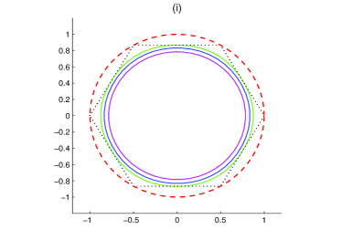
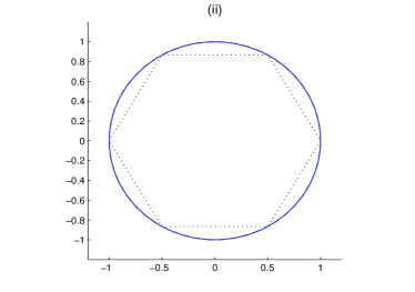
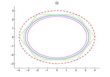
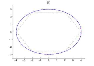
Figure 2: The green, blue and magenta coloured continuous lines represent the limit curves of scheme [3], [14] and [9], respectively in (i). The blue coloured continuous line represents the limit curve of proposed scheme in (ii).The reproduction of the unit circle and ellipse (the limit curves in continuous lines are obtained after three subdivision steps). The red coloured broken lines represent unit circles and ellipses and black coloured dotted lines represent control polygon.

It can be observed that certain functions like $\cos(\alpha.)$ and $\sin(\alpha.)$ can be reproduced by the proposed non-stationary schemes. In particular, if a set of equidistant point $f_{i}^{0}=\cos((i-\frac{1}{2})\alpha)$ and $\alpha=\frac{2\pi}{n}$, then the limit curve is the unit circle (see also figure 2). Similarly, $\sin((i-\frac{1}{2})\alpha)$ reproduces $\sin(\alpha.)$.

Proposition 6.1. The limit curves of the scheme (4.4) reproduces the functions $\cos(\alpha.)$ and $\sin(\alpha.)$ for the data points $f_{i}^{k}=\cos((i-\frac{1}{2})\frac{\alpha}{2^{k}})$ and $f_{i}^{k}=\sin((i-\frac{1}{2})\frac{\alpha}{2^{k}})$, respectively.
In other wards we have to show that for $k\geq 0$

(i) $f_{i}^{k}=\cos((i-\frac{1}{2})\frac{\alpha}{2^{k}})$, we have for $0\leq i\leq 2^{k}n$ as

$$f_{2i}^{k+1}=\cos\left(2i\frac{\alpha}{2^{k+1}}\right)~{}~{}~{}~{}and~{}~{}~{}~{}f_{2i}^{k+1}=\cos\left((2i+1)\frac{\alpha}{2^{k+1}}\right)$$

(ii) Similarly, for $f_{i}^{k}=\sin((i-\frac{1}{2})\frac{\alpha}{2^{k}})$, we have for $0\leq i\leq 2^{k}n$ as

$$f_{2i}^{k+1}=\sin\left(2i\frac{\alpha}{2^{k+1}}\right)~{}~{}~{}~{}and~{}~{}~{}~{}f_{2i}^{k+1}=\sin\left((2i+1)\frac{\alpha}{2^{k+1}}\right)$$

Proof: For any initial data of the form $f_{i}^{0}=\cos((i-\frac{1}{2})\alpha)$, it can be followed

$$f_{2i}^{1} = a_{0}^{(0)}f_{i}^{0}+a_{1}^{(0)}f_{i+1}^{0}$$

$$= \frac{\sin(\frac{3\alpha}{4})}{\sin\alpha}\cos((i-\frac{1}{2})\alpha)+\frac{\sin(\frac{\alpha}{4})}{\sin\alpha}\cos((i+\frac{1}{2})\alpha)=\cos\left(i\alpha\right)$$

Similarly, it can be followed for $k^{th}$ refinement

$$f_{2i}^{k}=\cos\left((2i)\frac{\alpha}{2^{k+1}}\right)$$

Analogously, it can also be proved.

$$f_{2i+1}^{k}=\cos\left((2i+1)\frac{\alpha}{2^{k+1}}\right)$$

Proof of part (ii) is similar. So, the scheme (4.4) can reproduce $\sin(\alpha.)$ for the initial data $f_{i}^{0}=\sin((i-\frac{1}{2})\alpha)$.

Proposition 6.2. The limit curves of the scheme (4.5) reproduces the functions $\cos(\alpha.)$ and $\sin(\alpha.)$ for the data points $f_{i}^{k}=\cos((i+\frac{1}{2})\frac{\alpha}{2^{k}})$ and $f_{i}^{k}=\sin((i+\frac{1}{2})\frac{\alpha}{2^{k}})$, respectively.
It can be proceed on same way. If a set of equidistant point $f_{i}^{0}=\cos((i-\frac{1}{2})\alpha)$ and $\alpha=\frac{2\pi}{n}$ can be chosen by the scheme (4.5), then the limit curve is the unit circle. Similarly, $\sin((i-\frac{1}{2})\alpha)$ reproduces $\sin(\alpha.)$.

6.2 Symmetry of Basis Limit Function

The basis limit function of the scheme is the limit function for the data

$$f^{0}_{i}=\left\{\begin{array}[]{rr}1,&i=0,\\ 0,&i\neq 0\\ \end{array}\right.$$

In order to prove that the basis limit function is symmetric about the Y-axis.

Theorem 6.1 The basis limit function F is symmetric about the Y-axis.
Proof. The symmetry of basis limit function can be followed on the same pattern following [15].

6.3 Special cases

It can be observed that the binary subdivision schemes presented in [3, 6, 9, 13, 14, 15, 16] are either the special cases or can be considered the non-stationary counterpart of the stationary schemes. (See also Table 1 and Table 2).

• The $C^{1}$ limiting curves can be obtained after taking $m=2$ in proposed algorithm. The obtained curves of scheme (5), taking $\alpha=\frac{\pi}{180}$, coincide with the limit curves of the famous corner cutting scheme of Chaikin [3].

• After setting $m=2$ and $m=3$ in proposed algorithm, the mask of 2-point and 3-point approximating non-stationary schemes, developed by Daniel and Shunmugaraj [6], can be obtained.

• The limit curves of 3-point stationary approximating scheme, introduced by Siddiqi and Ahamd [14], coincide with the limit curves of proposed 3-point scheme, after setting $m=3$ and $\alpha=\frac{\pi}{180}$.

• The limit curves of proposed 4-point scheme coincide with the limit curves obtained by the scheme  [9], for $m=4$ and $\alpha=\frac{\pi}{180}$.

• The limit curves of 5-point stationary approximating scheme introduced in [16] matched with the limit curves of proposed scheme, for setting $m=5$ and $\alpha=\frac{\pi}{180}$.

• The limit curves of 6-point stationary approximating scheme introduced in [13] matched with the limit curves of proposed scheme, for setting $m=6$ and $\alpha=\frac{\pi}{180}$.

• The proposed algorithm can also be considered as the non-stationary counterpart of $m$-point scheme developed by Siddiqi and Younis [15].

Table 1: The proposed algorithm can be considered as the non-stationary counterpart of the following existing binary approximating schemes, for different values of $m$.

Setting $m$	Scheme	Type	Continuity	Counterpart
2	2-point	Stationary	$C^{1}$	scheme [3]
3	3-point	Stationary	$C^{2}$	scheme [14]
4	4-point	Stationary	$C^{4}$	scheme [9]
5	5-point	Stationary	$C^{4}$	scheme [16]
6	6-point	Stationary	$C^{6}$	scheme [13]
$m$	$m$-point	Stationary	$C^{m-1}$	scheme [15]

Table 2: The following existing binary non-stationary approximating schemes can be considered the special case of proposed algorithm, for different values of $m$.

Setting $m$	Scheme	Type	Continuity	Coincides with
2	2-point	Non-stationary	$C^{1}$	scheme [6]
3	3-point	Non-stationary	$C^{2}$	scheme [6]

7 Conclusion

An algorithm of $m-$point binary approximating non-stationary subdivision scheme (for any integer $m\geq 2$) has been developed which generates the family of $C^{m-1}$ limiting curve, for $0<\alpha<\pi/3$. The construction of the algorithm is associated with trigonometric B-spline basis function. It is also evident from the examples that the limit curves of the proposed schemes coincide with the schemes presented in [3, 6, 14, 9, 13, 16]. So, the proposed algorithm, for different values of $m$, can be considered as the generalized form of the scheme [6] and non-stationary counterpart of the stationary schemes [3, 9, 13, 14, 16]. Moreover, the schemes produced by the algorithm can reproduce or regenerate the trigonometric polynomials, trigonometric splines and conic sections as well.

Figure 1: The continuous lines show the behavior of limit curves (after three subdivision steps) of the proposed scheme in blue, green, black and red colours, respectively, after setting $m=2,3,4$ and $5$. The blue, green, black and red coloured limit curves coincide with the schemes presented in [3], [6], [9] and [16], respectively. The dotted lines represent the control polygon

References

• [1] C. Beccari, G. Casciola and L. Romani, A non-stationary uniform tension controlled interpolating 4-point scheme reproducing conics, Comput. Aided. Geom. D. , 24(1) (2007), 1–9.
• [2] C. Beccari, G. Casciola and L. Romani, An interpolating 4-point $C^{2}$ ternary non- stationary subdivision scheme with tension control, Comput. Aided. Geom. D. , 24(4) (2007), 210–219.
• [3] G.M. Chaikin, An algorithm for high speed curve generation, Comput. Vision. Graph., 3(4) (1974), 346–349.
• [4] C. Conti and L. Romani, A new family of interpolatory non-stationary subdivision schemes for curve design in geometric modeling,in: Numerical Analysis and Applied Mathematics, International Conference Vol-I (2010).
• [5] C. Conti and L. Romani, Algebraic conditions on non-stationary subdivision symbols for exponential polynomial reproduction, J. Comput. Appl. Math. , 236 (2011), 543–556.
• [6] S. Daniel and P. Shunmugaraj, An approximating $C^{2}$ non-stationary subdivision scheme, Comput. Aided. Geom. D , 26 (2009), 810–821.
• [7] N. Dyn, J.A. Gregory and D. Levin, A 4-points interpolatory subdivision scheme for curve design, Comput. Aided. Geom. D. , 4(4) (1987), 257–268.
• [8] N. Dyn and D. Levin, Analysis of asymptotically equivalent binary subdivision schemes, J. Math. Anal. Appl. , 193 (1995), 594–621.
• [9] S.S. Siddiqi and N. Ahmad, An approximating $C^{4}$ stationary subdivision scheme, Eur. J. Sci. Res., 15(1) (2006), 97–102.
• [10] N. Dyn and D. Levin, Subdivision schemes in geometric modeling, Acta Numerica , 11 (2002), 73–144.
• [11] P.E. Koch, T. Lyche, M. Neamtu and L. Schumker, Control curves and knot insertion for trignometric splines, Adv. Comput. Math. , 3 (1995), 405–424.
• [12] J. Pana, S. Lin and X. Luo, A combined approximating and interpolating subdivision scheme with $C^{2}$ continuity, Appl. Math. Lett., 25(12) (2012), 2140–2146.
• [13] S.S. Siddiqi and N. Ahmad, A $C^{6}$ approximating subdivision scheme, Appl. Math. Lett., 21(7) (2008), 722–728.
• [14] S.S. Siddiqi and N. Ahmad, A new three-point approximating $C^{2}$ subdivision scheme, Appl. Math. Lett., 20(6) (2007), 707–711.
• [15] S.S. Siddiqi and M. Younis, Construction of m-point binary approximating subdivision schemes, Appl. Math. Lett. (2012), doi:10.1016/j.aml.2012.09.016.
• [16] S.S. Siddiqi and N. Ahmad, A new five-point approximating subdivision scheme, Int. J. Comput. Math., 85(1) (2008), 65–72.
Refer to caption
Refer to caption
Refer to caption
Refer to caption