Dynamics between order and chaos in conceptual models of glacial cycles

Abstract

The dynamics of glacial cycles is studied in terms of the dynamical systems theory. We explore the dependence of the climate state on the phase of the astronomical forcing by examining five conceptual models of glacial cycles proposed in the literature. The models can be expressed as quasiperiodically forced dynamical systems. It is shown that four of them exhibit a strange nonchaotic attractor (SNA), which is an intermediate regime between quasiperiodicity and chaos. Then, the dependence of the climate state on the phase of the astronomical forcing is not given by smooth relations, but constitutes a geometrically strange set. Our result suggests that SNA is a candidate for representing the dynamics of glacial cycles, in addition to well-known quasiperiodicity and chaos.

1 Introduction

The climate change in the Quaternary is characterized by alternations between cold (glacial) and warm (interglacial) periods, which are called glacial-interglacial cycles or alternatively glacial cycles. The aim of this article is to explore the dynamics of glacial cycles by examining conceptual models proposed in the literature.

Astronomical theories of ice ages, as typified by the Milankovitch theory (1941), attempt to explain glacial cycles based on the change in the incoming solar radiation (insolation) due to the long-term variations of the Earth’s orbital parameters. Assuming a constant solar output and a perfectly transparent atmosphere, the insolation $F$ at a given latitude and season is a function of the astro-insolation parameters: the eccentricity $e$ of the Earth’s orbit, the obliquity $\varepsilon$ (the inclination of the equator on the ecliptic), and the climatic precession $e\sin\tilde{\omega}$, where $\tilde{\omega}$ is the longitude of the perihelion measured from the moving vernal equinox (Berger 1978). That is, $F=F(e,\,\varepsilon,\,e\sin\tilde{\omega})$.

A motion expressed by a superposition of periodic motions of two or more incommensurate frequencies is called a quasiperiodic motion. In the studies of the Quaternary climate changes, the astro-insolation parameters are often assumed to be quasiperiodic (Berger 1978) as follows:

$$e=e_{0}+\sum E_{i}\cos(\lambda_{i}t+\phi_{i}),$$

$$\varepsilon=\varepsilon^{*}+\sum A_{i}\cos(f_{i}t+\delta_{i}),$$

$$e\sin\tilde{\omega}=\sum P_{i}\sin(\alpha_{i}t+\zeta_{i}).$$

Then, the insolation $F$ is also quasiperiodic in time (see Eq. (5)). The insolation variation $F(t)$ is known as astronomical forcing. The primary frequencies of astronomical forcing are approximately $1/19$ kyr^-1 and $1/23$ kyr^-1 for the climatic precession, and approximately $1/41$ kyr^-1 for the obliquity. The assumption of quasiperiodicity of astronomical forcing is considered to be approximately valid over the last several million years (Berger and Loutre 1991) but may not be valid beyond this period because of the intrinsic chaoticity of the planetary motion (Lasker 1989). However, since our study focuses on the glacial cycles during the past $0.7$ Myr after the mid-Pleistocene transition (Clark et al. 2006), we construct our theory on the assumption of quasiperiodic astronomical forcing.

Hays et al. (1976) presented strong evidence for astronomical theories of ice ages. They found the primary frequencies of astronomical forcing in the geological spectra of marine sediment cores. However, the dominant frequency in geological spectra is approximately $1/100$ kyr^-1, although this frequency component is negligible in the astronomical forcing. This is referred to as the “$100$ kyr problem.”

To understand the climate responses to astronomical forcing, several concepts related to the dynamical systems theory have been proposed in the literature. The linear response is a simple framework to explain the $41$, $23$, and $19$ kyr periodicities in the geological spectra. However, the linear response cannot appropriately account for the $100$ kyr periodicity (Hays et al. 1976). Ghil (1994) explained the appearance of the $100$ kyr periodicity as a nonlinear resonance to the combination tone $1/109$ kyr^-1 between precessional frequencies $1/19$ kyr^-1 and $1/23$ kyr^-1. Contrary to the linear resonance, the nonlinear resonance can occur even if the forcing frequencies are far from the internal frequency of the response system. Benzi et al. (1982) proposed stochastic resonance as a mechanism of the $100$ kyr periodicity, where the response to small external forcing is amplified by the effect of noise. Tziperman et al. (2006) proposed that the timing of deglaciations is set by the astronomical forcing via the phase-locking mechanism. If a phase locking occurs, the condition $qf=p_{1}f_{1}+p_{2}f_{2}+\cdots+p_{N}f_{N}$ is satisfied, where $f$ is the response frequency, $f_{1},\,f_{2},\,...,\,f_{N}$ are forcing frequencies, and $p_{1},\,p_{2},\,...,\,p_{N}$, and $q(\neq 0)$ are integers (Romeiras et al. 1987). De Saedeleer et al. (2013) suggested generalized synchronization (GS) to describe the relation between the glacial cycles and the astronomical forcing. GS means that there is a functional relation between the climate state and the state of the astronomical forcing. They also showed that the functional relation may not be unique for a certain model. However, the nature of the relation remains to be elucidated.

In this research, we analyze five conceptual models of glacial cycles proposed in the literature, and show that the dependence of the climate state on the phase of the astronomical forcing may not be given by smooth relations, but constitutes some geometrically strange set known as a strange nonchaotic attractor (SNA) (Grebogi et al. 1984; Kaneko 1984).

The remainder of this article is organized as follows. In Section 2, we review the notions of quasiperiodically forced systems and attractors. In Section 3, five models of glacial cycles are explained. In Section 4, we investigate attractors of the models numerically, and show possible relations between the climate state and the phase of the astronomical forcing. In Section 5, we show dynamical properties of the attractors. In Section 6, we mention an implication of the results. Section 7 concludes this article.

2 Quasiperiodically forced systems and attractors

2.1 Quasiperiodically forced systems

We consider the dynamics of glacial cycles in the framework of quasiperiodically forced dynamical systems. Let $\mathbb{T}^{N}=\mathbb{R}^{N}/(2\pi\mathbb{Z})^{N}$ be an $N$-dimensional torus. In general, quasiperiodically forced dynamical systems can be expressed as

$$\begin{split}\dot{\mathbf{\theta}}&=\mathbf{\omega},\ \ \ \ \ \ \ \ \theta\in\mathbb{T}^{N},\\ \dot{\mathbf{x}}&=\mathbf{g}\mathbf{(x},\mathbf{\theta}),\ \mathbf{x}\in\mathbb{R}^{M},\end{split}$$ (1)

where $\mathbf{\theta}=(\theta_{1},\theta_{2},...,\theta_{N})^{\mathrm{T}}$ is the phase of the drive subsystem, $\mathbf{x}=(x_{1},x_{2},...,x_{M})^{\mathrm{T}}$ is the state of the response subsystem, $\mathbf{g}\mathbf{(x},\mathbf{\theta})$ is a periodic function in each phase $\theta_{i}$, and $\mathbf{\omega}=(\omega_{1},\omega_{2},...,\omega_{N})^{\mathrm{T}}$ is a vector of incommensurate frequencies such that $k_{1}\omega_{1}+k_{2}\omega_{2}+\dots+k_{N}\omega_{N}=0$ does not hold for any set of integers, $k_{1}$, $k_{2}$, …, $k_{N}$, except for the trivial solution $k_{1}=k_{2}=\dots=k_{N}=0$. In the astronomical theory of climate change, $\theta$ corresponds to the phase of the astronomical forcing $F(t)$, and $\mathbf{x}$ corresponds to the climate state, as described in Section 3.

2.2 Attractors

Like most conceptual models of glacial cycles, we assume the existence of attractors in systems (1). An attractor is a compact set with a neighborhood such that, for almost every initial condition in this neighborhood, the limit set of the orbit as time tends to infinity is the attractor (Grebogi et al. 1984). The closure of set of initial conditions which approach an attractor as time tends to infinity is called the basin of attraction of the attractor. Note that the attractor of system (1) is a subset of $\mathbb{T}^{N}\times\mathbb{R}^{M}$. Thus, the dependence of the climate state on the phase of the astronomical forcing is represented by this attractor, after a certain transient time. In quasiperiodically forced systems (1), the following types of attractors typically appear: $N$-frequency quasiperiodic attractors, $L$-frequency quasiperiodic attractors with $L>N$, Strange nonchaotic attractors (SNAs), and chaotic attractors.

Lyapunov exponents give the mean exponential rates of divergence (or convergence) of nearby orbits. Although the Lyapunov exponents depend on initial conditions, they have the same set of values for almost every initial condition, under general circumstances. Such initial conditions or orbits which give the same set of values of the Lyapunov exponents are called typical. A chaotic attractor is an attractor for which typical orbits on the attractor have a positive Lyapunov exponent (Grebogi et al. 1984). That is, almost all orbits on the attractor have sensitive dependence on initial conditions. In quasiperiodically forced systems (1), an attractor is chaotic if the maximal conditional Lyapunov exponent (CLE) $\lambda$ is positive for typical orbits on the attractor, and nonchaotic otherwise. The maximal CLE $\lambda$ is defined as

$$\lambda=\lim_{t\to\infty}\frac{1}{t}\ln\frac{|\delta\mathbf{x}(t)|}{|\delta\mathbf{x}(0)|},$$

where $\delta\mathbf{x}(0)$ is an infinitesimal displacement of the orbit from $\mathbf{x}(0)$. The evolution of the infinitesimal displacement is given by the variational equation $\dot{\delta\mathbf{x}}=D_{\mathbf{x}}\mathbf{g}(\mathbf{x},\theta)\delta\mathbf{x}$.

An $N$-frequency quasiperiodic attractor is an attracting $N$-dimensional torus on which the motion is quasiperiodic. $N$-frequency quasiperiodic attractors are characterized by a negative maximal CLE, $\lambda<0$.

An $L$-frequency quasiperiodic attractor with $L>N$ is an attracting $L$-dimensional torus on which the motion is quasiperiodic. $L$-frequency quasiperiodic attractors with $L>N$ are characterized by a maximal CLE of zero, $\lambda=0$.

A strange nonchaotic attractor (SNA) is a strange attractor for which typical orbits have nonpositive Lyapunov exponents (Grebogi et al. 1984). The strange attractor is defined as an attractor which is not a finite set of points and is neither piecewise differentiable curve or surface, nor a volume bounded by a piecewise differentiable closed surface. SNAs are characterized by a negative maximal CLE, $\lambda<0$. It is proven that some SNAs are represented by a closure of graphs of almost everywhere discontinuous functions (Keller 1996; Alsedà and Costa 2009).

SNAs lie in an intermediate regime between quasiperiodicity and chaos. The power spectrum of an SNA is intermediate one between quasiperiodicity and chaos, namely, a singular continuous (fractal) spectrum (Feudel et al. 1996). SNAs are multifractal objects in the sense that the capacity dimension is larger than the information dimension (Ding et al. 1989; Hunt and Ott 2001). For comprehensive reviews of SNAs, refer to Prasad et al. (2001) as well as Feudel et al. (2006).

In the remainder of this article, we will not encounter examples of $L$-frequency quasiperiodic attractors with $L>N$, and sometimes $N$-frequency quasiperiodic attractors are simply referred to as quasiperiodic attractors.

2.3 Examples of $N$-frequency quasiperiodic attractors and an SNA

A quasiperiodically forced map is regarded as a stroboscopic map obtained by sampling the state of the continuous-time system (1) at time intervals corresponding to one of the forcing frequencies. Let us consider the following quasiperiodically forced map studied by Glendinning (2002):

$$\begin{split}\theta(n+1)&=\theta(n)+\omega\pmod{1},\\ x(n+1)&=2\sigma(\alpha+\cos 2\pi\theta(n))\tanh x(n),\end{split}$$ (2)

where $(\theta,x)\in[0,1)\times\mathbb{R}$, $n\in\mathbb{Z}$, $\omega\in\mathbb{R}\setminus\mathbb{Q}$, and $\sigma$ and $\alpha$ are non-negative parameters.

Figure 1(a) shows the quasiperiodic attractors for $\sigma=1.2$, $\alpha=1.001$, and $\omega=(\sqrt{5}-1)/2$ (solid lines). Each attractor is represented by a graph of a smooth function. If we denote the attractor in the region $x>0$ by $x=\phi(\theta)$, the attractor in the other region is $x=-\phi(\theta)$ because of the symmetry $x\to-x$. The line $x=0$ is an unstable invariant set, namely, a repellor. In this case, the repellor constitutes the basin boundary of two attractors.

Figure 1(b) shows the SNA for $\sigma=1.2$, $\alpha=0.8$, and $\omega=(\sqrt{5}-1)/2$. The SNA is represented by the closure of two graphs $x=\varphi(\theta)$ and $x=-\varphi(\theta)$ having following properties (Glendinning 2002; Keller 1996):
(i) $\varphi(\theta)\geq 0$ for all $\theta\in[0,1)$;
(ii) the union of two graphs $x=\varphi(\theta)$ and $x=-\varphi(\theta)$
is invariant under the map;
(iii) typical conditional Lyapunov exponents on the graphs are negative;
(iv) $\varphi(\theta)$ is discontinuous at almost all $\theta\in[0,1)$;
(v) $\varphi(\theta)$ is upper semi-continuous;
(vi) $\varphi(\theta)=0$ on a dense, but measure zero, set of values of $\theta\in[0,1)$.

Figure 1: Attractors in map (2): a Quasiperiodic attractors for $\sigma=1.2$, $\alpha=1.001$, and $\omega=(\sqrt{5}-1)/2$ (upper and lower solid lines). The maximal CLE is $\lambda=-0.3677$ for each attractor. b SNA for $\sigma=1.2$, $\alpha=0.8$, and $\omega=(\sqrt{5}-1)/2$ (dots). The maximal CLE is $\lambda=-0.2124$. In each panel, the dashed line $x=0$ is the unstable invariant set

Unlike quasiperiodic attractors, SNAs contain some repellors in themselves (Stark 1997). See the repellor $x=0$ embedded in the SNA in Fig. 1(b). Due to such repellors, the orbits on SNAs become temporarily unstable and sensitive to perturbations, as shown in Section 5.

2.4 Numerical characterization of strangeness of attractors

SNAs and $N$-frequency quasiperiodic attractors can be numerically distinguished by the phase sensitivity exponent (Pikovsky and Feudel 1995) or by the parameter sensitivity exponent (Nishikawa and Kaneko 1996). First, let us consider the case of the continuous-time system (1). The phase sensitivity function $\Gamma(t)$ of variable $x_{j}$ with respect to variable $\theta_{i}$ is defined as

$$\Gamma(t)=\min_{\{\mathbf{x}(0),\theta(0)\}}\left\{\max_{0\leq\tau\leq t}\left|\frac{\partial x_{j}(\tau)}{\partial\theta_{i}(0)}\right|\right\}.$$

The derivative $\partial x_{j}(\tau)/\partial\theta_{i}(0)$ characterizes the sensitivity of $x_{j}$ with respect to a change of $\theta_{i}$. This derivative is obtained by integrating

$$\frac{d}{dt}\frac{\partial x_{j}}{\partial\theta_{i}(0)}=\sum_{k=1}^{M}\frac{\partial g_{j}(\mathbf{x},\mathbf{\theta})}{\partial x_{k}}\frac{\partial x_{k}}{\partial\theta_{i}(0)}+\frac{\partial g_{j}(\mathbf{x},\mathbf{\theta})}{\partial\theta_{i}(0)},$$ (3)

along the solution ($\mathbf{\theta}(t),\mathbf{x}(t)$). For SNAs, the phase sensitivity function grows as $\Gamma(t)\simeq t^{\mu}$ with $\mu>0$, where $\mu$ is called the phase sensitivity exponent. On the other hand, for $N$-frequency quasiperiodic attractors, $\Gamma(t)$ is bounded and $\mu=0$.

Assume that function $\mathbf{g}(\mathbf{x},\theta)$ contains some parameter, say $\alpha$. The parameter sensitivity function $\Psi(t)$ of variable $x_{i}$ with respect to parameter $\alpha$ is defined as

$$\Psi(t)=\min_{\{\mathbf{x}(0),\theta(0)\}}\left\{\max_{0\leq\tau\leq t}\left|\frac{\partial x_{j}(\tau)}{\partial\alpha}\right|\right\}.$$

The derivative $\partial x_{j}(\tau)/\partial\alpha$ characterizes the sensitivity of $x_{j}$ with respect to a change of $\alpha$. This derivative is obtained by integrating

$$\frac{d}{dt}\frac{\partial x_{j}}{\partial\alpha}=\sum_{k=1}^{M}\frac{\partial g_{j}(\mathbf{x},\mathbf{\theta})}{\partial x_{k}}\frac{\partial x_{k}}{\partial\alpha}+\frac{\partial g_{j}(\mathbf{x},\mathbf{\theta})}{\partial\alpha},$$ (4)

along the solution ($\mathbf{\theta}(t),\mathbf{x}(t)$). For SNAs, the phase sensitivity function grows as $\Psi(t)\simeq t^{\nu}$ with $\nu>0$, where $\nu$ is called the parameter sensitivity exponent. On the other hand, for $N$-frequency quasiperiodic attractors, $\Psi(t)$ is bounded and $\nu=0$.

For discrete-time systems, such as Eq. (2), the methods for characterizing the strangeness of attractors are almost the same except that time evolutions corresponding to Eqs. (3) and (4) become discrete in time (Pikovsky and Feudel 1995; Nishikawa and Kaneko 1996).

Figure 2 shows the time evolutions of the phase sensitivity function $\Gamma(n)$ and the parameter sensitivity function $\Psi(n)$ with respect to $\alpha$ for the attractors in Fig. 1. The functions $\Gamma(n)$ and $\Psi(n)$ saturate for large $n$ for the quasiperiodic attractors, but show power-law divergences with exponents $\mu=1.03$ and $\nu=0.99$ for the SNA.

Figure 2: a Phase sensitivity function $\Gamma(n)$ for the quasiperiodic attractors of map (2) with $\sigma=1.2$, $\alpha=1.001$, and $\omega=(\sqrt{5}-1)/2$ (open square) and for the SNA with $\sigma=1.2$, $\alpha=0.8$, and $\omega=(\sqrt{5}-1)/2$ (filled circle). b Paramater sensitivity function $\Psi(n)$ for the same attractors

3 Models

3.1 Astronomical insolation forcing

Milankovitch (1941) considered the high-latitude northern hemisphere summer insolation as a decisive factor for glaciations. We use the insolation $F(t)$ at $65^{\circ}$N on the day of the summer solstice in the simulations of all the models. For simplicity in computation, the insolation $F(t)$ is calculated using the following formula given in De Saedeleer et al. (2013):

$$F(t)=\frac{1}{a}\sum_{i=1}^{N}[s_{i}\sin(\omega_{i}t)+c_{i}\cos(\omega_{i}t)],$$

where $N=35$ is the number of different frequencies $\omega_{i}$ included in the sum. The values of frequencies $\omega_{i}$ are those in Berger (1978). The coefficients $s_{i}$ and $c_{i}$ are obtained by linear regression on the insolation values calculated after Berger (1978) (De Saedeleer et al. 2013). To make the paper self-contained, the values of $\omega_{i}$, $s_{i}$, and $c_{i}$ are listed in Table 3 in Appendix 1. The parameter $a$ is a scale factor, the value of which is different among models. The top panel of Fig. 4 shows the insolation $F(t)$ normalized to have zero-mean and unit variance (with $a=23.58$ W/m²).

Introducing variables $\theta_{i}(t)=\omega_{i}t$ ($i=1,2,...,N$), the above equation for $F(t)$ can be written as

$$\begin{split}F(t)&=\frac{1}{a}\sum_{i=1}^{N}[s_{i}\sin\theta_{i}(t)+c_{i}\cos\theta_{i}(t)],\\ \dot{\theta}_{i}&=\omega_{i},\ \ \ \theta_{i}(0)=0\ \ \ (i=1,2,...,N).\end{split}$$ (5)

Note that $\theta_{i}$ are the phase variables of the astronomical forcing in climate models.

3.2 Conceptual models of glacial cycles

3.2.1 Saltzman–Maasch model

Saltzman and Maasch (1990) introduced a global model of the late Cenozoic climate. We will refer to this model as SM90. The model consists of differential equations for the global ice volume $x$, the atmospheric CO₂ concentration $y$, and the global mean deep water temperature $z$, where $x$, $y$, and $z$ are dimensionless and denote deviations from $1$ Myr averages. Neglecting stochastic perturbations, the model is written in the following deterministic from:

$$\begin{split}\tau\dot{x}&=-x-y-vz-uF(t),\\ \tau\dot{y}&=-pz+ry+sz^{2}-wyz-z^{2}y,\\ \tau\dot{z}&=-q(x+z),\end{split}$$ (6)

where $t$ is the time in kiloyears, and $\tau=10$ kyr. The parameters $p$, $q$, $r$, $s$, and $w$ are freely chosen, but the remaining parameters $u$ and $v$ are functions of the other parameters. The insolation forcing $F(t)$ is given by Eq. (5) with $a=23.58$ W/m².

Saltzman and Maasch (1990) simulated glacial cycles for the last $500$ kyr by choosing the parameter values as set A in Table 1. Hargreaves and Annan (2002) estimated the parameter values of SM90 as set B using a data assimilation technique.

Table 1: Sets of parameter values used for the SM90 and MS90 models

Set	$p$	$q$	$r$	$s$	$u$	$v$	$w$
A	$1.0$	$2.5$	$0.9$	$1.0$	$0.6$	$0.2$	$0.5$
B	$0.82$	$4.24$	$0.95$	$0.53$	$0.32$	$0.02$	$0.66$
C	$1.0$	$1.2$	$0.8$	$0.8$	$0.7$	$0.0$	$0.0$

3.2.2 Maasch–Saltzman model

Prior to the SM90 model, Maasch and Saltzman (1990) studied one of their previous models. This older model, which we call the MS90 model, can be obtained from the SM90 model by setting $v=w=0$. The other parameter values are chosen as set C in Table 1.

3.2.3 Crucifix–De Saedeleer–Wieczorek model

One of the simplest systems that exhibit self-sustained oscillations is the van der Pol oscillator. With slight modifications and addition of the insolation forcing to the van der Pol oscillator, Crucifix (2012) introduced the following model:

$$\begin{split}\tau\dot{x}&=-[y+\beta+\gamma F(t)],\\ \tau\dot{y}&=-\alpha[y^{3}/3-y-x],\end{split}$$ (7)

where $x$ denotes the global ice volume, and $y$ is a conceptual variable for realizing self-sustained oscillations. The insolation forcing $F(t)$ is given by Eq. (5) with $a=11.77$ W/m². For the unforced case $\gamma=0$, Eq. (7) has a stable equilibrium point for $|\beta|>1$ and a stable limit cycle for $|\beta|<1$. Following Crucifix (2012), the parameters are set as $\alpha=30.0$, $\beta=0.75$, $\gamma=0.4$, and $\tau=36.0$ kyr.

The dynamical properties of Eq. (7) were extensively studied by De Saeldeleer, Crucifix, and Wieczorek (2013). Thus, we refer to Eq. (7) as the CSW model.

3.2.4 Paillard–Parrenin model

Paillard and Parrenin (2004) proposed an oscillator model of glacial cycles involving the Antarctic ice-sheet influence on bottom water formation. The model, which we call the PP04 model, consists of equations for the global ice volume $x$, extent of the Antarctic ice sheet $y$, and atmospheric CO₂ concentration $z$ as follows:

$$\begin{split}\tau_{x}\dot{x}&=-pz-qF(t)+r-x,\\ \tau_{y}\dot{y}&=x-y,\\ \tau_{z}\dot{z}&=\alpha F(t)-\beta x+\gamma H(-w)+\delta-z,\\ w&=ax-by-cI(t)+d,\end{split}$$ (8)

where $F(t)$ is the summer solstice insolation at 65^∘N given by Eq. (5) with $a=23.58$ W/m², and $I(t)$ is the insolation at 60^∘S on February 21. The Heaviside function in the original PP04 model is approximated as $H(x)=1/2+\arctan(1000x)/\pi$ for simplicity of the dynamical systems analysis. The parameters are set as $\tau_{x}=15$ kyr, $\tau_{y}=12$ kyr, $\tau_{z}=5$ kyr, $p=1.3$, $q=0.5$, $r=0.8$, $\alpha=0.15$, $\beta=0.5$, $\gamma=0.5$, $\delta=0.4$, $a=0.3$, $b=0.7$, $c=0$, and $d=0.27$. The choice $c=0$ does not change the timing of terminations; it only affects the qualitative agreement with geological records (Paillard and Parrenin 2004).

3.2.5 Imbrie–Imbrie model

Imbrie and Imbrie (1980) proposed a piecewise-linear model for the glacial cycles as follows:

$$\begin{split}\tau\dot{x}&=\left\{\begin{split}(1+b)(F(t)-x)\,\,\,\mbox{if}\,\,F(t)\geq x,\\ (1-b)(F(t)-x)\,\,\,\mbox{if}\,\,F(t)<x,\end{split}\right.\end{split}$$

where $x$ corresponds to a loss in the global ice volume. The variable $F(t)$ is assumed to be the summer solstice insolation at 65^∘N given by Eq. (5) with $a=23.58$ W/m² (cf. Paillard 2001). The parameters are tuned as $\tau=17$ kyr and $b=0.6$. For simplicity of the dynamical systems analysis, we deal with a smoothed system,

$$\tau\dot{x}=[1+b\tanh k(F(t)-x)](F(t)-x).$$ (9)

If the steepness parameter $k$ is large enough, the solution of Eq. (9) converges to that of the original model. We set $k=10$ in this study.

4 Dynamical systems analysis

4.1 Synchronization under the same astronomical forcing

In what follows, $\mathbf{x}(t)$ represents the climate state at time $t$ for each model described in the previous section. First, we check the dependence of solutions on initial climate states under the same astronomical forcing $F(t)$. We simulate $10^{4}$ solutions $\mathbf{x}^{(i)}(t)$ ($i=1,\,2,\,...,\,10^{4}$), starting from random initial states $\mathbf{x}^{(i)}(t_{0})$ at time $t_{0}=-20$ Myr, under the same astronomical forcing $F(t)$. For these solutions, we calculate the maximum distance from the average of the ensemble,

$$\Delta_{\max}(t)=\max_{1\leq i\leq 10^{4}}\left|\mathbf{x}^{(i)}(t)-\langle\mathbf{x}^{(i)}(t)\rangle\right|.$$

We assume that typical solutions converge to the same solution, i.e., synchronize, under the same astronomical forcing if $\Delta_{\max}(t)\to 0$ as $t\to\infty$. Figure 3 shows the behavior of $\Delta_{\max}(t)$ for each model.

Figure 3: Convergence of $10^{4}$ solutions for each model: the maximum distance from the average of the ensemble $\Delta_{\max}(t)=\max_{1\leq i\leq 10^{4}}\left|\mathbf{x}^{(i)}(t)-\langle\mathbf{x}^{(i)}(t)\rangle\right|$ vs. elapsed time $t-t_{0}$. All solutions start from random initial states at time $t_{0}=-20$ Myr. Note that the time scale is different for each panel

In each model except for the SM90-B model, typical solutions synchronize after a certain transient time. This result implies that the attractor is unique at least except for the SM90-B model. It should be mentioned that the transient time is longer than the duration of the Quaternary, approximately 2.58 Myr, in the SM90-A and MS90 models (see Fig. 3).

4.2 Simulated ice volume over the last 700 kyr

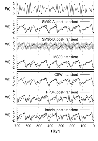
Figure 4: Top panel: Normalized insolation $F(t)$ at 65^∘N on the day of summer solstice. Other panels: Simulated normalized ice volume $V(t)$ (solid lines) for the models described in Section 3. The $\delta^{18}O$ record of the LR04 stack is also shown for comparison (dashed lines). Post-transient solutions are presented for the SM90-A, SM90-B, PP04, and Imbrie models, and transient solutions are presented for the MS90 and CSW models

Figure 4 shows the simulated normalized ice volume $V(t)$ over the last 700 kyr (solid line) for each model. The $\delta^{18}O$ record of the LR04 stack is also shown by a dashed line for comparison (Lisiecki and Raymo 2005). In the SM90-A, PP04, and Imbrie models, synchronized solutions after each transient period are well accorded with the $\delta^{18}O$ record; however, in the MS90 and CSW models, synchronized solutions after each transient period are not accorded with the $\delta^{18}O$ record, but only some transient solutions agree with the $\delta^{18}O$ record. In the SM90-B model, solutions starting from different initial states do not synchronize. This result indicates that the SM90-B model exhibits chaotic solutions.

Actually we find coexistence of a quasiperiodic attractor and a chaotic attractor for the SM90-B model. The quasiperiodic attractor originates in a stable equilibrium of the unforced system $(x,y,z)=$(-0.282, 0.277, 0.282). The basin of attraction of this quasiperiodic attractor is much smaller than that of the chaotic attractor, and the amplitude of the quasiperiodic solution is also much smaller than that of the chaotic solutions. Thus, we do not focus on this quasiperiodic solution.

4.3 Types of attractors

We analyze types of attractors using the maximal CLE $\lambda$, the phase sensitivity exponent $\mu$, and the parameter sensitivity exponent $\nu$. As shown in Table 2, the maximal CLE $\lambda$ is positive for the SM90-B model, and is negative for all the other models. Thus, the SM90-B model is chaotic, and all the other models are nonchaotic. This result is consistent with that of convergence experiments.

Table 2: Characteristic exponents and types of attractors for the different models. The asterisk ($\ast$) indicates that the sensitivity exponents are undefined for the SM90-B model.

Models	$\lambda$ [kyr-1]	$\mu$	$\nu$	Attractor
SM90-A	$-0.0014$	1.06	1.15	SNA
SM90-B	$+0.0020$	$\ast$	$\ast$	Chaotic
MS90	$-0.0005$	0.95	1.09	SNA
CSW	$-0.016$	1.10	1.13	SNA
PP04	$-0.0093$	1.09	1.08	SNA
Imbrie	$-0.046$	0.0	0.0	Quasiperiodic

The next question is whether the attractors are strange or not. Figure 5(a) shows the phase sensitivity functions $\Gamma(t)$ of $x$ with respect to phase variable $\theta_{4}$ for the models with nonchaotic attractors, and Fig. 5(b) shows the parameter sensitivity functions $\Psi(t)$ of $x$ with respect to parameter $u$ for the SM90-A and MS90 models, parameter $\beta$ for the CSW model, and parameter $b$ for the Imbrie model. Here, the functions $\Gamma(t)$ and $\Psi(t)$ are calculated for a set of $20$ initial conditions. For the Imbrie model, the functions $\Gamma(t)$ and $\Psi(t)$ saturate as time increases, but for the other models, the functions $\Gamma(t)$ and $\Psi(t)$ grow in power-laws with exponents $\mu>0$ and $\nu>0$, respectively. Table 2 shows the values of $\mu$ and $\nu$, which are estimated from the power-law behaviors for $t>10^{4}$. Therefore, the attractors of the SM90-A, MS90, CSW, and PP04 models are SNAs, and the attractor of the Imbrie model is a quasiperiodic attractor.

Figure 5: a Phase sensitivity function $\Gamma(t)$ of $x$ with respect to a phase variable $\theta_{4}$. b Parameter sensitivity function $\Psi(t)$ of $x$ with respect to $u$ for the SM90-A and MS90 models, parameter $\beta$ for the CSW model, and parameter $b$ for the Imbrie model

4.4 Illustration of attractors by simplification of astronomical forcing

Since the astronomical forcing $F(t)$ in Eq. (5) has high degrees of freedom, namely, $N=35$ in our study, the attractors in climate models have at least 35 dimensions, which are too high-dimensional to be visualized. To capture the geometric features of these attractors, we illustrate attractors for simplified astronomical forcing. Leaving only the 23.7 kyr ($i=1$) and 19.1 kyr ($i=3$) precession terms and the 41.0 kyr ($i=4$) obliquity term, we simplify the astronomical forcing $F(t)$ as

$$F(t)=\frac{1}{a_{\{1,3,4\}}}\sum_{i\in\{1,3,4\}}[s_{i}\sin(\omega_{i}t)+c_{i}\cos(\omega_{i}t)].$$

These three frequency components constitute 78% of the original astronomical forcing with respect to standard deviations. The scale factor is $a_{\{1,3,4\}}=9.08$ W/m² for the CSW model and $a_{\{1,3,4\}}=18.3$ W/m² for the other models. For this simplified forcing, we obtain the same type of attractor for each model although the values of characteristic exponents are different from the original values: an SNA with $\lambda\approx-0.0004$, $\mu=1.39$, and $\nu=1.43$ for the SM90-A model, a chaotic attractor with $\lambda\approx 0.0025$ for the SM90-B model, an SNA with $\lambda\approx-0.00012$, $\mu=1.09$, and $\nu=1.35$ for the MS90 model, an SNA with $\lambda\approx-0.0088$, $\mu=1.13$, and $\nu=1.10$ for the CSW model, an SNA with $\lambda\approx-0.0089$, $\mu=1.07$, and $\nu=0.94$ for the PP04 model, and a quasiperiodic attractor with $\lambda\approx-0.046$ and $\mu=\nu=0$ for the Imbrie model. A number of frequency components are needed to obtain the attractors with almost the same values of characteristic exponents as the original attractors. Figure 6 shows the dependence of the characteristic exponents on the number of frequency components $N$ in the astronomical forcing $F(t)$ for the case of the SM90-A model, where the scale factor $a$ is changed depending on $N$ to normalize $F(t)$. Roughly speaking, $N\geq 9$ is necessary and almost sufficient to approximate the original attractor of the SM90-A model.

Figure 6: Dependence of the characteristic exponents on the number of frequency components $N$ for the case of the SM90-A model. Top panel: The maximal conditional Lyapunov exponent $\lambda$. Bottom panel: The phase sensitivity exponent $\mu$ and the parameter sensitivity exponent $\nu$. The numerical calculation procedures for these exponents are the same as in Section 4.3. The attractor for $N=3$ is a quasiperiodic attractor, whose tiny but nonzero sensitivity exponents are due to finite computation time

To visualize the simplified attractors we construct stroboscopic maps. Observing the system at the moments $t_{n}=2\pi n/\omega_{1}+\mbox{const.}$ ($n\in\mathbb{Z}$), where phase $\theta_{1}(t)$ attains a constant value, the system reduces to a stroboscopic map ($\theta_{3}(t_{n}),$ $\theta_{4}(t_{n})$, $\mathbf{x}(t_{n})$) $\mapsto$ ($\theta_{3}(t_{n+1}),$ $\theta_{4}(t_{n+1})$, $\mathbf{x}(t_{n+1})$). Figure 7 shows the attractors of the simplified models. Each panel presents the projection of the attractor on the space ($\theta_{3}(t_{n})/2\pi$, $\theta_{4}(t_{n})/2\pi$, $x(t_{n})$).

Figure 7: Attractors of each model for the simplified astronomical forcing. Each panel shows the projection of the attractor on the space ($\theta_{3}/2\pi$, $\theta_{4}/2\pi$, $x$)

The SM90-A, MS90, CSW, and PP04 models exhibit SNAs, and the dependence of the climate state on the phase of the astronomical forcing is not given by smooth relations, but constitutes a geometrically strange set. Moreover, the dependence seems to be discontinuous almost everywhere. For the Imbrie model, the attractor is quasiperiodic, and the dependence is given by a smooth graph. For the SM90-B model, the attractor is chaotic, and the dependence constitutes a geometrically strange set, as in the case of SNAs.

5 Dynamical properties of the attractors

5.1 Asymptotic behavior and transient behavior

The difference in asymptotic behavior between chaotic and nonchaotic attractors has been shown in the previous section. If a climate model has a chaotic attractor, solutions sensitively depend on initial climate states $\mathbf{x}(t_{0})$. On the other hand, if a climate model has an SNA or a quasiperiodic attractor, only one or several synchronized solutions are obtained, regardless of initial climate states $\mathbf{x}(t_{0})$, after a certain transient time.

In the previous section, we mentioned that some of the models have a considerably long transient time for synchronization, compared to the Quaternary period. For such a model, transient behavior is important in practice. Let us compare the transient dynamics of the SM90-A, SM90-B, and MS90 models. Since the SM90-B model has the maximal CLE of 0.002 kyr^-1, we can observe the divergence of nearby orbits within about 500 kyr (the so-called Lyapunov time). On the other hand, for the nonchaotic models (SM90-A and MS90), we do not observe such a divergence but a slower convergence process of nearby orbits. That is, the behavior of nearby orbits is different between the chaotic and nonchaotic attractors. However, a chaotic model and a nonchaotic model would not be distinguishable within 1 million years if the maximal CLE of the chaotic model is less than 0.001 kyr^-1.

5.2 Sensitivity to dynamical noise

Khovanov et al. (2000) stated that SNAs and quasiperiodic attractors differ in sensitivity to perturbations. We illustrate the difference by simulating the CSW and Imbrie models in the presence of noise. In the former, we add independent white Gaussian noises $\xi_{i}(t)$ ($i=x$ or $y$) to the right-hand sides of Eq. (7), respectively, where $\langle\xi_{i}(t)\rangle=0$, $\langle\xi_{i}(t)\xi_{j}(t^{\prime})\rangle=\sigma^{2}\delta_{ij}\delta(t-t^{\prime})$, and $\sigma=0.1~{}\mbox{kyr}^{1/2}$. In the latter, we add a white Gaussian noise $\xi_{x}(t)$ with the same average and standard deviation to the right-hand side of Eq. (9).

Figure 8: Sensitivity of climate models to perturbations: a Ice volume $x(t)$ simulated by the CSW model with noise (red) and without noise (black). b Ice volume $x(t)$ simulated by the CSW model for $\tau=36.0$ kyr (black) and for $\tau=36.1$ kyr (red). The other parameter values are the same as in Section 3.2.3. c The finite-time CLE $\lambda_{T}(t)$ of the unperturbed trajectory of the CSW model in panels a and b. $T=70$ kyr. d Loss of ice volume $x(t)$ simulated by the Imbrie model with noise (black) and without noise (red). e Loss of ice volume $x(t)$ simulated by the Imbrie model for $\tau=17$ kyr (black) and for $\tau=19$ kyr (red). The other parameter values are the same as in Section 3.2.5. f The finite-time CLE $\lambda_{T}(t)$ of the unperturbed trajectory of the Imbrie model in panels d and e. $T=70$ kyr

Figure 8(a) shows two trajectories of the CSW model simulated with and without noises, and Fig. 8(d) shows those of the Imbrie model. In each model, perturbed and unperturbed trajectories start from the same initial climate state $\mathbf{x}(t_{0})$ at $t_{0}=-1.5$ Myr, and the noise is added to each system from $t=0$ kyr. The CSW model is more sensitive to noise than the Imbrie model because of the local instability of SNA. To characterize the local instability of attractors, let us define a finite-time CLE

$$\lambda_{T}(t)=\frac{1}{T}\ln\frac{|\delta\mathbf{x}(t+T)|}{|\delta\mathbf{x}(t)|}.$$

The finite-time CLE $\lambda_{T}(t)$ gives the rate of exponential divergence of nearby orbits during the time interval $[t,t+T]$. Note that $\lambda_{T}(t)$ converges to the maximal CLE $\lambda$ as $T\to\infty$. For SNAs, the finite-time CLE $\lambda_{T}(t)$ can be positive even for large $T$ with nonzero probability (Pikovsky and Feudel 1995). Thus, the orbits of SNAs are sensitive to perturbations in time intervals with $\lambda_{T}(t)>0$. Figures 8(a) and 8(c) show that the perturbed trajectory occasionally deviates after the finite-time CLE $\lambda_{T}(t)$ becomes positive, where $T=70$ kyr. This local instability may be attributed to a repellor embedded in SNA as mentioned in Section 2. Such a temporary loss of synchronization has been shown also in another model of glacial cycles (Crucifix 2011). The frequency and the duration of desynchronization increase as the magnitude of noise $\sigma$ increases. Therefore, the orbits of SNAs and those of chaotic attractors might be indistinguishable under large dynamical noise.

On the other hand, for quasiperiodic attractors, the finite-time CLE $\lambda_{T}(t)$ takes only negative values for large $T$. As a result, the orbits of quasiperiodic attractors are robust to perturbations in comparison with those of SNAs. Figures 8(d) shows that the Imbrie model is robust to the same magnitude of noise that can cause larger deviations of trajectories in the CSW model. For the Imbrie model, the finite-time CLE $\lambda_{T}(t)$ with $T=70$ kyr is always negative as shown in Fig. 8(f).

If a climate model has a nonchaotic attractor in the absence of noise, there can be a relation from the phase of the astronomical forcing to the climate state. The existence of such an intact phase relation is assumed when we refine a time scale of a paleoclimate record based on astronomical cycles (the so-called orbital tuning). However, the above results suggest that such a phase relation is rather robust for quasiperiodic attractors but not robust for SNAs.

6 Discussion

Let us mention an implication of this study for paleoclimate modeling. The notion of SNAs will be helpful for understanding apparently-contradictory properties of conceptual models of glacial cycles. In a number of previous studies, it is reported that a model of glacial cycles is sensitive to subtle changes in parameter values although the model is insensitive to initial conditions (for example, Weertman 1978; Oerlemans 1982; Paillard 2001; Ganopolski and Calov 2011; Crucifix 2013). In some models, such parameter sensitivity may be attributed to thresholds with discontinuity (Paillard 2001). However, parameter sensitivity can arise in continuous models when they have SNAs. Figure 8(b) shows strong parameter sensitivity of the CSW model with SNA. The black line represents the original solution for $\tau=36.0$ kyr, and the red line represents the solution for $\tau=36.1$ kyr (the parameter change is only 2.8% of the original value). Figure 8(e) shows weak parameter sensitivity of the Imbrie model with quasiperiodic attractor. The black line represents the original solution for $\tau=17$ kyr, and the red line represents the solution for $\tau=19$ kyr (the parameter change is 10.5% of the original value).

In a recent paper, Crucifix (2013) investigates the causes of parameter sensitivity inherent in various conceptual models of glacial cycles, which can make the prediction of ice ages difficult (see also Added note). Crucifix (2013) attributes the parameter sensitivity to two causes: complicated bifurcation structures with numerous frequency-locking tongues and abrupt changes of attractors with respect to subtle changes in parameter values. We conjecture that such abrupt changes of attractors are due to a property of SNAs with strange geometry. The validation of this conjecture needs detailed bifurcation analyses and will be an important future study.

7 Conclusion

We analyzed five conceptual models of glacial cycles in the framework of the dynamical systems theory. The SM90-A, MS90, CSW, and PP04 models exhibit a strange nonchaotic attractor (SNA), and the dependence of the climate state on the phase of the astronomical forcing is not given by smooth relations, but constitutes a geometrically strange set. The SM90-B model exhibits a chaotic attractor, and the dependence of the climate state on the phase of the astronomical forcing is not given by smooth relations, but constitutes a geometrically strange set. The Imbrie model exhibits a quasiperiodic attractor, and the dependence of the climate state on the phase of the astronomical forcing is given by a smooth graph. These results suggest that SNA is a candidate for representing the dynamics of glacial cycles, in addition to well-known quasiperiodicity and chaos. Since SNAs have repellors in themselves, the orbits on SNAs are locally unstable. Therefore, if the real climate system has an SNA, the orbit will be temporarily sensitive to perturbations when the finite-time conditional Lyapunov exponent is positive.

The analysis in this paper was restricted to spatially zero-dimensional models that can be approximated by smooth dynamical systems. A hybrid dynamical system is a system that has both continuous and discrete dynamics (Aihara and Suzuki 2010). A number of ice age models are expressed as hybrid dynamical systems, more precisely, hybrid automata (van der Schaft and Schumacher 2000). For example, the models by Paillard (1998), Parrenin and Paillard (2003), and Ashkenazy and Tziperman (2004) are hybrid automata. The Imbrie and PP04 models are also hybrid dynamical systems but can be approximated by smooth dynamical systems because they are especially piecewise affine systems. The description of the dynamics appearing in hybrid automata models or in more complicated models with spacial dimensions is still unclear. This problem should be studied in the future.

Added note

After the submission of our article, we came to know a discussion paper submitted at about the same time, which mentions SNAs in an ice age model (Crucifix M, Why could ice age be unpredictable? Clim Past Discuss 9:1053-1098, 2013). The author demonstrates the appearance of SNAs in the CSW model for simplified forcing with two frequencies, which is different from the forcing used in our article. The verification method of SNAs is also different between two articles. We use the maximal conditional Lyapunov exponent and the sensitivity exponents. On the other hand, Crucifix (2013) uses the pullback section method described in De Saedeleer et al. (2013). Thus, the results obtained by Crucifix and by us are distinguishable and complementary to each other. The discussion in Section 6 is motivated by the paper (Crucifix 2013).

Appendix 1: Parameter values for the insolation formula

The parameter values for the insolation formula (5) given by De Saedeleer et al. (2013) are listed in Table 3 to make the paper self-contained. The frequencies and coefficients are arranged in descending order of their power $s_{i}^{2}+c_{i}^{2}$.

Table 3: Parameter values for the insolation formula of De Saedeleer et al. (2013)

Index $i$	$\omega_{i}$ [rad/kyr]	$s_{i}$ [W/m2]	$c_{i}$ [W/m2]
1	0.264933601588513	-15.549049332290400	-9.704062871105320
2	0.280151350350945	15.431955636170100	4.752472711315250
3	0.331110950251899	9.099224935273400	-10.611524488739001
4	0.153249478547167	-11.228737681512399	3.516820752112410
5	0.328024059125949	-7.870653840136690	6.615442460635030
6	0.326211762560183	0.813786144754451	-4.526414080992460
7	0.158148666238883	-3.824993714675400	-0.761851750263805
8	0.269742342439881	0.069044850431486	-3.316392609695580
9	0.117190147169570	2.288148059560660	1.802337026846230
10	0.332923246817665	1.440507707859670	1.063392860501200
11	0.150162587421217	1.549041763533020	-0.088394191276982
12	0.217333905941751	0.380973541305497	-1.463017119992100
13	0.155061775112933	-1.297700819564400	-0.635152963728496
14	0.371638925683567	0.925324276580528	-1.020667586721540
15	0.324937167999999	-0.576082669762308	1.186695727393380
16	0.275366617473065	0.997628846513796	-0.362906496840039
17	0.211709630908568	-0.810768209286259	-0.577980646565494
18	0.156336369673117	-0.918358442095885	0.196083726889428
19	0.334197841377850	0.346906064369828	-0.648189701487285
20	0.259396912994958	0.339477750517033	-0.560509461538342
21	0.323124871434233	-0.378637986107629	0.527217891742183
22	0.148350290855451	0.256895610735773	-0.524697312305024
23	0.111684123041346	-0.428006728186239	0.357006342316690
24	0.336010137943616	-0.421809264016129	0.324327509437558
25	0.274551083291250	-0.441772417569753	0.289576210423804
26	0.126901871803777	0.257509918217341	-0.377639794223366
27	0.177861471704732	-0.161827722328271	-0.362683869407858
28	0.206924898030688	-0.335783913402678	-0.019479215012864
29	0.212525165090383	0.267659228540196	0.128915417116900
30	0.004899187691716	-0.160479848721994	0.059407796893426
31	0.418183080135680	-0.018488406464501	0.109632390175297
32	0.433400828898112	-0.004919921945456	-0.106148873639336
33	0.229992875969202	0.069618973318896	0.074623171406128
34	0.311398144786051	0.013835372762118	0.030473666884042
35	0.306498957094334	0.024734974816962	0.014046439534097

References

- (1) Aihara K, Suzuki H (2010) Theory of hybrid dynamical systems and its applications to biological and medical systems. Phil Trans R Soc A 368:4893-4914
- (2) Alsedà L, Costa S (2009) On the definition of strange nonchaotic attractor. Fund Math 206:23-39
- (3) Ashkenazy Y, Tziperman E (2004) Are the 41kyr glacial oscillations a linear response to Milankovitch forcing. Quat Sci Rev 23:1879-1890
- (4) Benzi A, Parisi G, Sutera A, and Vulpiani A (1982) Stochastic resonance in climatic change. Tellus 34:10-16
- (5) Berger AL (1978) Long-term variations of daily insolation and quaternary climatic changes. J Atmos Sci 35:2362-2367
- (6) Berger A, Loutre MF (1991) Insolation values for the climate of the last 10 million years. Quat Sci Rev 10:297-317 (1991).
- (7) Brindley J, Kapitaniak T (1992) Inhibition of chaotic behaviour in coupled models of atmospheric dynamics and climate evolution. In: Chaotic Dynamics, Theory and Practice, T. Bountis (ed.), NATO ASI, Plenum, pp. 317-326
- (8) Clark PU, Archer D, Pollard D, Blum JD, Rial JA, Brovkin V, Mix AC, Pisias NG, Roy M (2006) The middle Pleistocene transition: characteriscs, mechanisms, and implications for long-term changes in atmospheric pCO2. Quat Sci Rev 25:3150-3184
- (9) Crucifix M (2011) How can a glacial inception be predicted? Holocene 21:831-842
- (10) Crucifix M (2012) Oscillators and relaxation phenomena in Pleistocene climate theory. Philos Trans R Soc A 370:1140-1165
- (11) Crucifix M (2013) Why could ice age be unpredictable? Clim Past Discuss 9:1053-1098
- (12) De Saedeleer B, Crucifix M, Wieczorek S (2013) Is the astronomical forcing a reliable and unique pacemaker for climate? A conceptual model study. Clim Dyn 40:273-294
- (13) Ding M, Grebogi C, Ott E (1989) Dimensions of strange nonchaotic attractors. Phys Lett A 137:167-172
- (14) Feudel U, Kuznetsov S, Pikovsky A (2006) Strange Nonchaotic Attractors. World Scientific, Singapore.
- (15) Feudel U, Pikovsky A, Politi A (1996) Renormalization of correlations and spectra of a strange non-chaotic attractor. J Phys A Math Gen 29:5297-5311
- (16) Ganopolski A, Calov R (2011) The role of orbital forcing, carbon dioxide and regolith in 100 kyr glacial cycles. Clim Past, 7:1415-1425
- (17) Ghil M (1994) Cryothermodynamics: the chaotic dynamics of paleoclimate. Physica D 77:130-159
- (18) Glendinning P (2002) The non-smooth pitchfork bifurcation. Discrete and Continuous Dynamical Systems-Series B 6(4):1-7
- (19) Grebogi C, Ott E, Pelikan S, Yorke JA (1984) Strange attractors that are not chaotic. Physica D 13:261-268
- (20) Hargreaves JC, Annan JD (2002) Assimilation of paleo-data in a simple Earth system model. Clim Dyn 19:371-381
- (21) Hays JD, Imbrie J, Shackleton NJ (1976) Variations in the earth’s orbit: pacemaker of ice ages. Science 194:1121-1132
- (22) Hunt BR, Ott E (2001) Fractal properties of robust strange nonchaotic attractors. Phys Rev Lett 87:254101
- (23) Huybers PJ (2009) Pleistocene glacial variability as a chaotic response to obliquity forcing. Climate of the Past 5(3): 481-488
- (24) Imbrie J, Imbrie JZ (1980) Modelling the climatic response to orbital variations. Science 207:943-953
- (25) Kaneko K (1984) Fractalization of torus. Prog Theor Phys 71:1112-1115
- (26) Keller G (1996) A note on strange nonchaotic attractors. Fund Math 151:139-148
- (27) Khovanov IA, Khovanova NA, McClintock PVE, Anishchenko VS (2000) The effect of noise on strange nonchaotic attractors. Phys Lett A 268:351-322
- (28) Laskar J, Robutel P, Joutel F, Boudin F, Gastineau M, Correia ACM, Levrard B (2004) A long-term numerical solution for the insolation quantities of the earth. Astronom Astroph 428:261-285
- (29) Lisiecki LE, Raymo ME (2005) A Pliocene-Pleistocene stack of 57 globally distributed benthic d18O records. Paleoceanography 20:PA1003
- (30) Maasch KA, Saltzman B (1990) A low-order dynamical model of global climatic variability during the full Pleistocene. J Geophys Res 95: 1955-1963
- (31) Milankovitch M (1941) Kanon der Erdbestrahlung und seine Anwendung auf das Eiszeitenproblem. Königlich Serbische Akademie, Belgrade
- (32) Nicolis C (1987) Long-term climatic variability and chaotic dynamics. Tellus 39A:1-9
- (33) Nishikawa T, Kaneko K (1996) Fractalization of a torus as a strange nonchaotic attractor. Phys Rev E 54:6114-6124
- (34) Oerlemans J (1982) Glacial cycles and ice-sheet modelling. Climate Change 4:353-374
- (35) Paillard D (1998) The timing of Pleistocene glaciations from a simple multiple-state climate model. Nature 391:378-381
- (36) Paillard D (2001) Glacial cycles: toward a new paradigm. Rev Geophys 39(3):325-346
- (37) Paillard D, Parrenin F (2004) The Antarctic ice sheet and the triggering of deglaciations. Earth Planet Sci Lett 227:263-271
- (38) Pikovsky A, Feudel U (1995) Characterizing strange nonchaotic attractors. Chaos 5(1):253-260
- (39) Prasad A, Negi SS, Ramaswamy R (2001) Strange nonchaotic attractors. Int J Bifurcat Chaos 11(2):291-309
- (40) Ramaswamy R (1997) Synchronization of strange nonchaotic attractors. Phys Rev E 56:7294
- (41) Rial JA (2004) Abrupt climate change: chaos and order at orbital and millennial scales. Global and Planetary Change 41:95-109
- (42) Romeiras FJ, Bondeson A, Ott E, Antonsen TM Jr, Grebogi C (1987) Quasiperiodically forced dynamical systems with strange nonchaotic attractors. Physica D 26:277-294
- (43) Saltzman B, Maasch KA (1990) A first-order global model of late Cenozoic climatic change. Trans R Soc Edinburgh Earth Sci 81:315-325
- (44) Saltzman B, Verbitsky MY (1992) Asthenospheric ice-load effects in a global dynamical-system model of the Pleistocene climate. Clim Dyn 8:1-11
- (45) Saltzman B, Verbitsky MY (1993) Multiple instabilities and modes of glacial rhythmicity in the Plio-Pleistocene: a general theory of late Cenozoic climatic change. Clim Dyn 9:1-15
- (46) Stark J (1997) Invariant graphs for forced systems. Physica D 109:163-179
- (47) Tziperman E, Raymo ME, Huybers P, Wunsch C (2006) Consequences of pacing the Pleistocene 100 kyr ice ages by nonlinear phase locking to Milankovitch forcing. Paleoceanography 21:PA4206
- (48) van der Schaft A, Schumacher H (2000) An Introduction to Hybrid Dynamical Systems. Springer, London
- (49) Weertman J (1976) Milankovitch solar variation radiations and ice age ice sheet sizes. Nature 261:17-20