The Traffic Phases of Road Networks

Abstract

We study the relation between the average traffic flow and the vehicle density on road networks that we call 2D-traffic fundamental diagram. We show that this diagram presents mainly four phases. We analyze different cases. First, the case of a junction managed with a priority rule is presented, four traffic phases are identified and described, and a good analytic approximation of the fundamental diagram is obtained by computing a generalized eigenvalue of the dynamics of the system. Then, the model is extended to the case of two junctions, and finally to a regular city. The system still presents mainly four phases. The role of a critical circuit of non-priority roads appears clearly in the two junctions case. In Section 4, we use traffic light controls to improve the traffic diagram. We present the improvements obtained by open-loop, local feedback, and global feedback strategies. A comparison based on the response times to reach the stationary regime is also given. Finally, we show the importance of the design of the junction. It appears that if the junction is enough large, the traffic is almost not slowed down by the junction.

1 Introduction

The purpose of this paper is the discussion of the traffic phases appearing in road networks. These phases appear clearly on what we call the 2D traffic fundamental diagram. This diagram gives the relation between the average flow and the car density in the network. The 2D traffic fundamental diagram is an extension to road networks of the well-known fundamental diagram studied mainly for a unique road in traffic literature such as in (Derrida and Evans, 1994; Fukui and Ishibashi, 1996; Nagel and Schreckenberg, 1992; Blank, 2000; Wang et al., 2000; Chowdhury et al., 2000; Helbing, 2001; Lotito et al., 2005). This relation between the car density and the car flow has been observed on a highway since 1935 by Greenshields (1935).

Microscopic traffic on a road network has been studied in statistical physics with a cellular automata point of view in (Chowdhury et al., 2000; Biham et al., 1992; Molera et al., 1995b; Cuesta et al., 1993; Molera et al., 1995a) similar to the modeling done here. These works are mainly about numerical simulations showing a threshold density where blocking appears for somewhat different modeling, often stochastic. The case of two roads with one junction without turning possibilities with a stochastic modeling has been studied in detail in (Fukui and Ishibashi, 1996, 2001a, 2001b). In (Brockfeld et al., 2001), the traffic light optimization of a city is done with an automatic control point of view.

Recently, other attempts to extend this fundamental diagram to the 2D cases have been done in (Geroliminis and Daganzo, 2007; Daganzo and Geroliminis, 2008; Geroliminis and Daganzo, 2008; Buisson and Ladier, 2009; Helbing, 2009) in traffic literature.

Daganzo and Geroliminis (2008), using a variational traffic theory (Daganzo, 2005; Geroliminis and Daganzo, 2007, 2008), have shown the existence of a concave macroscopic fundamental diagram first on a ring, then on a network using an aggregation method. Experimental studies (e.g. Buisson and Ladier, 2009) have shown that heterogeneity in traffic measurements may have a strong impact on the shape of the fundamental diagram built using the aggregation approach of Daganzo and Geroliminis (2008).

More recently, Helbing (2009), using queuing theory, has derived fundamental diagrams for a traffic model with junctions in the saturated and unsaturated cases.

Here we propose a new 2D traffic model obtained from Petri net modeling and maxplus algebra. This paper belongs to a sequence of works presented in conferences (Farhi et al., 2005, 2007), available online (Farhi, 2009a, b), a thesis (Farhi, 2008), and a companion paper (Farhi et al., 2009). We give the first full synthesis of what we have understood on the traffic phases. In (Farhi et al., 2005, 2007; Farhi, 2009b, 2008; Farhi et al., 2009) the models are presented using Petri nets and maxplus algebra formalisms. Here we avoid these formalisms and use only dynamical systems in the standard algebra framework. Our point of view is close to the cellular automata one where interactions of a large number of simplified vehicles are studied in asymptotic regimes. Our point of view is different from the two approaches (Daganzo-Geroliminis and Helbing) discussed previously. Our models are simpler but the systems can be analyzed more deeply. In particular the fundamental diagram is obtained (numerically or analytically) for the complete set of possible densities. The different traffic phases can be deduced from the obtained diagram instead of making a specific analysis for each traffic situation (under or over saturated traffic), as for example, in (Helbing, 2009).

We consider various closed regular road networks cut in cells which can contain at most one car. At a junction, a car leaving can turn. To enter the junction, we consider the priority to the right policy (a vehicle gives way to vehicles approaching from the right at intersections) or the use of traffic lights with various strategies. The roads are one-way streets without possibility of overtaking. A car in a cell enters the next cell as soon as it is freed. We observe through simulation or by mathematical analysis (in the simplest case) four phases :

• Free phase: This phase corresponds to low densities. After a finite transitional time, the vehicles separate enough to be able to move freely. The average flow is equal to the density.

• Saturation phase: This phase corresponds to average densities. The junctions serve with their maximal flow. There is no jam downstream of the junctions. The average flow is constant (independent of the density).

• Recession phase: This phase corresponds to densities large enough to jam places downstream of the junctions. The average flow decreases with the density.

• Freeze phase: This phase corresponds to high densities, where the number of vehicles is large enough to fill a circuit of roads. Once such a full circuit is constituted, the traffic is frozen and the average flow vanishes.

The simplest case studied is a system of two circular roads with only one junction managed with the priority to the right rule. In this case, the dynamics is given. It is additively homogeneous of degree one. We can prove the existence of an average flow which is close to a generalized eigenvalue obtained analytically. We are particularly interested in the dependence of these quantities with respect to the density, but the ratio ($r$) between the number of cells of the non-priority road and the number of cells of the priority road also plays an important role in the determination of the four phases.

Then, we study the case of four roads with two junctions. We show numerically that the fundamental diagram has the same shape as in the previous case, but now $r$ has to be interpreted as the ratio between the length of a non-priority road circuit and the length of a priority road circuit. When we extend the analysis to a larger network, the same kind of results persists.

The four phases exist in the presence of traffic light control, but the length of the saturation phase can be enlarged and the freeze phase reduced, almost without any impact on the free phase. Moreover, we show that the number of cells of the junction plays an important role. In our simple model, if we consider a junction of two cells, instead of one cell, we suppress the saturation phase and multiply by two the maximal flow.

Throughout this paper, we consider closed networks with a fixed number of vehicles and wait until a stationary or periodic regime is established to compute the average flow as a function of a given density. Nevertheless, the fundamental diagrams have a sense for open systems when the density evolves slowly with respect to the car speed. The diagram can be useful to describe the behavior of zones of real towns with homogeneous structure of roads and junctions.

Numerical simulations are done with the Scicoslab software. They use the maxplus arithmetic of this software very useful to describe large dynamical systems in a matrix may. These simulations have played an important role to understand the different phases of the system before being able to derive them sometimes analytically.

2 Traffic modeling and analysis of two circular roads with one junction

We consider a circular traffic system of two roads with one junction, in the shape of the numeral 8 , as shown on Figure 1. At the junction, the priority to the right rule is applied to enter, and the vehicles have the possibility to go straight or to turn. Thus, the northwest road has priority over the southeast road.

Each road is cut in cells. We denote by $m$ and $n$ the sizes (in number of cells) of the priority and of the non-priority roads, respectively. The cells are numbered. The junction is considered as a special cell having two inputs and two outputs with two sub-cells inside ($n$ and $n+m$ containing the vehicles going respectively West and South); see Figure 1. Each cell, including the junction, can contain at most one vehicle. In a unit of time, on the roads outside the junction, a vehicle moves to the cell ahead if the latter is free, and stays unmoved otherwise. At the junction, the proportion of vehicles leaving and going west is equal to the proportion of vehicles going south, and thus equal to $1/2$. To enter the junction, the priority to the right rule is applied. That is, a vehicle coming from the north has priority over a vehicle coming from the east.

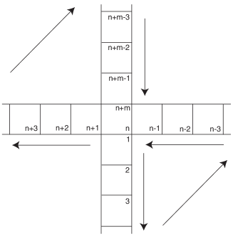
Figure 1: Two circular roads crossing on a junction with possibility of turning.

2.1 The Dynamics

The car positions at the initial time (time $0$) are given by numbers $a_{i},1\leq i\leq n+m$. For $i\neq n,n+m$, $a_{i}$ gives the number of cars in the cell $i$ at time $0$. $a_{n}$ (resp. $a_{n+m}$) gives the number of cars being in the junction at time $0$, and that are going west (resp. south). Therefore the total number of cars in the junction at time $0$ is $a_{n}+a_{n+m}$. To describe the car dynamics on this system, we use the variable $x_{i}^{k}$ which denotes :
– for $i\neq n,n+m$, the cumulative car inflow into cell $i$ up to time $k$,
– for $i=n$, the cumulative inflow of vehicles coming from the non-priority road (from cell $n-1$), into the junction up to time $k$,
– for $i=n+m$, the cumulative inflow of vehicles coming from the priority road (from cell $n+m-1$), into the junction up to time $k$.

1. For each cell $i$, $i\neq 1,n,n+1,n+m$, the cumulative car inflow into cell $i$ up to time $k+1$, denoted by $x_{i}^{k+1}$ satisfies:

   • $x_{i}^{k+1}$ is less than or equal to $a_{i-1}+x_{i-1}^{k}$, which is the number of vehicles present at cell $i-1$ at time $0$, given by $a_{i-1}$, plus the cumulative car inflow into cell $i-1$ up to time $k$, given by $x_{i-1}^{k}$.

   • $x_{i}^{k+1}$ is less than or equal to $1-a_{i}+x_{i+1}^{k}$, which is the number of free places at cell $i$ at time $0$, given by $1-a_{i}$, plus the cumulative car outflow of cell $i$ (that is the cumulative car inflow into cell $i+1$ up to time $k$), given by $x_{i+1}^{k}$.

   • $x_{i}^{k+1}$ is given by one of these two bounds since a car enters a cell as soon as possible.

   Thus, we have:

   $$x_{i}^{k+1}=\min\{a_{i-1}+x_{i-1}^{k},1-a_{i}+x_{i+1}^{k}\}.$$ (1)

2. For cell 1:

   • $x_{1}^{k+1}$ is less than or equal to $a_{n+m}+(x_{n}^{k}+x_{n+m}^{k})/2$, which is the number of vehicles being in the junction and going south at time $0$, given by $a_{n+m}$, plus one half of the total cumulative car inflow into the junction up to time $k$, given by $(x_{n}^{k}+x_{n+m}^{k})/2$.

   • $x_{1}^{k+1}$ is less than or equal to $1-a_{1}+x_{2}^{k}$ which is the number of free places in cell $1$ at time $0$, given by $1-a_{1}$, plus the cumulative car outflow of cell $1$ (that is the cumulative car inflow into cell $2$ up to time $k$), given by $x_{2}^{k}$.

   • $x_{1}^{k+1}$ is given by one of these two bounds since a car enters a cell as soon as possible.

   Hence:

   $$x_{1}^{k+1}=\min\{a_{n+m}+\frac{x_{n}^{k}+x_{n+m}^{k}}{2}\;,1-a_{1}+x_{2}^{k}\}.$$ (2)

   If we want to maintain the integer property of counting events and obtain a discrete version of equation (2), we could use the dynamics:

   $$x_{1}^{k+1}=\min\{a_{n+m}+\left\lceil\frac{x_{n}^{k}+x_{n+m}^{k}}{2}\right\rceil\;,1-a_{1}+x_{2}^{k}\},$$ (3)

   where $\lceil\cdot\rceil$ is the rounding up operator to the nearest integer. Equation (3), together with equation (5) given below, tell that, with respect to the total counting of vehicles entered the junction, the odd vehicles go south and the even vehicles go west.

3. For cell $n+1$, similarly with cell 1, we obtain:

   $$x_{n+1}^{k+1}=\min\{a_{n}+\frac{x_{n}^{k}+x_{n+m}^{k}}{2}\;,1-a_{n+1}+x_{n+2}^{k}\}.$$ (4)

   $$x_{n+1}^{k+1}=\min\{a_{n}+\left\lfloor\frac{x_{n}^{k}+x_{n+m}^{k}}{2}\right\rfloor\;,1-a_{n+1}+x_{n+2}^{k}\}.$$ (5)

   where $\lfloor\cdot\rfloor$ is the rounding down operator to the nearest integer.

4. For cell $n+m$:

   • $x^{k+1}_{n+m}$ is less than or equal to $a_{n+m-1}+x_{n+m-1}^{k}$, which is the number of vehicles present at cell $n+m-1$ at time $0$, given by $a_{n+m-1}$, plus the cumulative car inflow into cell $n+m-1$ up to time $k$, given by $x_{n+m-1}^{k}$.

   • $x^{k+1}_{n+m}$ is less than or equal to $1-a_{n}-a_{n+m}+x_{1}^{k}+x_{n+1}^{k}-x_{n}^{k}$, which is the number of free places in the junction at time $0$, given by $1-a_{n}-a_{n+m}$, plus the cumulative car inflow into cell $1$ up to time $k$, given by $x_{1}^{k}$, plus the cumulative car inflow into cell $n+1$ up to time $k$, given by $x_{n+1}^{k}$, minus the cumulative car inflow into cell $n$ up to time $k$, given by $x_{n}^{k}$. Indeed, $1-a_{n}-a_{n+m}+x_{1}^{k}+x_{n+1}^{k}-x_{n}^{k}$ gives the number of entry authorizations by the North into the junction up to time $k$ (there is an authorization when the junction is free). The number $x_{1}^{k}+x_{n+1}^{k}$ gives the cumulative inflow of cars having left the junction up to time $k$. The number $x_{n}^{k}$ is subtracted here because entry authorizations to the junction are also used by vehicles entering from the East, and here, vehicles coming from the North have priority to use these authorizations.

   • $x^{k+1}_{n+m}$ is given by one of these two bounds since a car enters a cell as soon as possible.

   Thus:

   $$x_{n+m}^{k+1}=\min\{a_{n+m-1}+x_{n+m-1}^{k}\;,1-a_{n}-a_{n+m}+x_{1}^{k}+x_{n+1}^{k}-x_{n}^{k}\}.$$ (6)

5. For cell $n$:
   Similarly with cell $n+m$, we obtain :

   $$x_{n}^{k+1}=\min\{a_{n-1}+x_{n-1}^{k}\;,1-a_{n}-a_{n+m}+x_{1}^{k}+x_{n+1}^{k}-x_{n+m}^{k+1}\}.$$ (7)

   where we have to subtract the number of authorizations used by entering cars from the North up to time $k+1$, since these cars have priority.

The dynamics of the whole system, in the continuous case (equations (2) and (4) are considered rather than equations (3) and (5)), is then given by:

$$x_{i}^{k+1}=\min\{a_{i-1}+x_{i-1}^{k},1-a_{i}+x_{i+1}^{k}\},\;i\neq 1,n,n+1,n+m\;,$$ (8)

$$x_{n}^{k+1}=\min\{a_{n-1}+x_{n-1}^{k}\;,1-a_{n}-a_{n+m}+x_{1}^{k}+x_{n+1}^{k}-x_{n+m}^{k+1}\}\;,$$ (9)

$$x_{n+m}^{k+1}=\min\{a_{n+m-1}+x_{n+m-1}^{k}\;,1-a_{n}-a_{n+m}+x_{1}^{k}+x_{n+1}^{k}-x_{n}^{k}\}\;,$$ (10)

$$x_{1}^{k+1}=\min\{a_{n+m}+(x_{n}^{k}+x_{n+m}^{k})/2\;,1-a_{1}+x_{2}^{k}\}\;,$$ (11)

$$x_{n+1}^{k+1}=\min\{a_{n}+(x_{n}^{k}+x_{n+m}^{k})/2\;,1-a_{n+1}+x_{n+2}^{k}\}\;.$$ (12)

The parameters $a_{i}$ satisfy the constraints

$$\begin{cases}0\leq a_{i}\leq 1,\;1\leq i\leq n+m\;,\\ 0\leq a_{n}+a_{n+m}\leq 1.\end{cases}$$ (13)

The car density denoted by $d$ is given by

$$d=\frac{1}{n+m-1}\sum_{i=1}^{n+m}a_{i}.$$ (14)

In Table 1, we show a short simulation of the system (8)–(12), with the parameters $n=m=5$, $a=[0,1,0,1,0,1,0,0,1,0]$, and the initial condition $x^{0}=[0,0,0,0,0,0,0,0,0,0]$.

Time	$x_{1}$	$x_{2}$	$x_{3}$	$x_{4}$	$x_{5}$	$x_{6}$	$x_{7}$	$x_{8}$	$x_{9}$	$x_{10}$
0	0	0	0	0	0	0	0	0	0	0
1	0	0	1	0	0	0	1	0	0	1
2	1/2	0	1	0	0	1/2	1	1	0	1
3	1/2	1/2	1	0	1	1/2	3/2	1	1	1
4	1	1/2	1	1	1	1	3/2	3/2	1	1
5	1	1	3/2	1	1	1	2	3/2	1	2

Table 1: A simulation of the system (8)–(12) (continuous dynamics).

In table 2, we show a simulation of the discrete version of this system; that is a simulation of ((8), (9), (10), (3), (5)).

Time	$x_{1}$	$x_{2}$	$x_{3}$	$x_{4}$	$x_{5}$	$x_{6}$	$x_{7}$	$x_{8}$	$x_{9}$	$x_{10}$
0	0	0	0	0	0	0	0	0	0	0
1	0	0	1	0	0	0	1	0	0	1
2	1	0	1	0	0	0	1	1	0	1
3	1	1	1	0	1	0	1	1	1	1
4	1	1	1	1	1	1	1	1	1	1
5	1	1	2	1	1	1	2	1	1	2

Table 2: A simulation of the system ((8), (9), (10), (3), (5)) (discrete dynamics).

Using the discrete dynamics, we can compute the car positions on the roads. Let us denote by $y_{i}^{k}$ the boolean variable telling whether if there is a car in cell $i$ at time $k$ ($y_{i}^{k}=1$) or not ($y_{i}^{k}=0$). The value $y_{n}^{k}$ (resp. $y_{n+m}^{k}$) gives the presence of a car in the junction going west (resp. south). The presence of a car in the junction, no matter if it is going south or west, is given by $y_{n}^{k}+y_{n+m}^{k}$. The values of $y_{i}^{k},1\leq i\leq n+m,k\in\mathbb{N}$ are deduced from the values of $x_{i}^{k},1\leq i\leq n+m,k\in\mathbb{N}$ as follows:

$$\begin{cases}y_{i}^{k}=a_{i}+x_{i}^{k}-x_{i+1}^{k},\quad i\neq n,n+m,&\\ y_{n+m}^{k}=a_{n+m}+\lceil(x_{n}^{k}+x_{n+m}^{k})/2\rceil-x_{1}^{k},&\\ y_{n}^{k}=a_{n}+\lfloor(x_{n}^{k}+x_{n+m}^{k})/2\rfloor-x_{n+1}^{k}.&\end{cases}$$ (15)

Note that, with the initial condition $x^{0}=0$ (which is natural here since $x_{i}^{k}$ is a cumulative flow) we have $y_{i}^{0}=a_{i},\forall 1\leq i\leq n+m$. This is also true for any initial condition $x^{0}$ satisfying $x_{p}^{0}=x_{q}^{0},\forall 1\leq p,q\leq n+m$. Indeed, this property comes from the additive homogeneity of degree $1$ of the dynamical system, as it is mentioned below. In Table 3, we give the car positions computed using (15) where $x_{i}^{k},1\leq i\leq n+m,\;\;0\leq k\leq 5$ are the values given in Table 2.

	Non-priority road				Junction		Priority road
	$\longrightarrow$				West	South	$\longleftarrow$
Time	$y_{1}$	$y_{2}$	$y_{3}$	$y_{4}$	$y_{5}$	$y_{10}$	$y_{9}$	$y_{8}$	$y_{7}$	$y_{6}$
0	0	1	0	1	0	0	1	0	0	1
1	0	0	1	1	0	1	0	0	1	0
2	1	0	1	1	0	0	0	1	0	0
3	0	1	1	0	1	0	1	0	0	0
4	0	1	0	1	0	0	1	0	0	1
5	0	0	1	1	0	1	0	0	1	0

Table 3: Car positions deduced from the simulation of the discrete dynamics.

Let us remark that some car flow bounds can be obtained. Outside the junction, at most one vehicle can pass through each cell in two units of time (one time unit to enter the cell, one time unit to leave the cell). Thus the flow is bounded by $1/2$ on the roads. The junction having to serve the two roads it is natural to think that the junction induces a bound of 1/4 on the flow. This is justified in Theorem 1 below.

To discuss the properties of the system (8)–(12), we recall some definitions. Let $g:~{}\mathbb{R}^{p}\to\mathbb{R}^{p}$. The dynamical system $x^{k+1}=g(x^{k})$ is additively homogeneous of degree $1$ if $g$ satisfies $\forall x\in\mathbb{R}^{n},\forall\alpha\in\mathbb{R},g(\alpha\textbf{1}\normalsize+x)=\alpha\textbf{1}\normalsize+g(x),$ where we denote $\textbf{1}\normalsize={}^{t}(1,1,...,1)$. The dynamical system $x^{k+1}=g(x^{k})$ is monotone if $g$ satisfies $\forall x,y\in\mathbb{R}^{p},x\leq y\Rightarrow g(x)\leq g(y).$ It admits a growth rate if the vector $\chi\in\mathbb{R}^{p}$, defined by $\chi=\lim_{k\to+\infty}x^{k}/k$, exists. It admits an additive eigenvalue if there exists $x\in\mathbb{R}^{p}$ such that $\lambda+x=g(x)$. When $\chi_{i}=\chi_{j},\forall 1\leq i,j\leq p$, we may also say, by abuse of language, that the growth rate $\chi$ is any of these components.

The dynamical system (8)–(12) is additively homogeneous of degree $1$ but not monotone (because of equations (9) and (10)). It is known (Gaubert and Gunawardena, 2004) that if an additively homogeneous system is monotone and connected, then the average growth rate of the dynamical system is unique (independent of the initial state of the system), and its components are equal and coincide with its unique additive eigenvalue. In our case, we have the following result (see (Farhi et al., 2009; Farhi, 2008) for the proof).

Theorem 1.

The system (8)-(12) with the initial condition $x^{0}=0$ have the following properties :

1. The trajectories of the states are non-negative and non-decreasing.

2. The distances between any pair of states stay bounded :
   $\exists c\in\mathbb{R},\sup_{k}|x_{i}^{k}-x_{j}^{k}|\leq c,\forall i,j$.

3. If a growth rate $\chi$ exists, then $\chi\leq 1/4$.

From Theorem 1 and from the property of homogeneity, it is easy to apply the ergodic theorem and prove the existence of a growth rate; see (Farhi et al., 2009). Moreover, the eigenvalue problem can be solved explicitly as a function of the vehicle density; see (Farhi, 2008, 2009b). In our case this eigenvalue is not equal to the growth rate, but we can derive a good approximation (justified by numerical simulations) of the growth rate from its analytic expression.

2.2 The eigenvalue as a function of the density

We are interested in this subsection by solving the additive eigenvalue problem associated to the dynamical system (8)–(12). The objective of determining the eigenvalue is to compare it to the growth rate of the dynamical system, which is interpreted in terms of traffic as the average car flow. We will see that, although the eigenvalue is different from the average car flow, it gives a good approximation of it. This approximation helps a lot to identify and understand all the phases of traffic.

The eigenvalue problem associated to the dynamical system (8)–(12) is the computation of the couple $(\lambda,x)$ solution of:

$$\lambda+x_{i}=\min\{a_{i-1}+x_{i-1},1-a_{i}+x_{i+1}\},\quad i\neq 1,n,n+1,n+m\;,$$ (16)

$$\lambda+x_{n}=\min\{a_{n-1}+x_{n-1}\;,1-a_{n}-a_{n+m}+x_{1}+x_{n+1}-(\lambda+x_{n+m})\}.$$ (17)

$$\lambda+x_{n+m}=\min\{a_{n+m-1}+x_{n+m-1}\;,1-a_{n}-a_{n+m}+x_{1}+x_{n+1}-x_{n}\}\;,$$ (18)

$$\lambda+x_{1}=\min\{a_{n+m}+(x_{n}+x_{n+m})/2\;,1-a_{1}+x_{2}\}\;,$$ (19)

$$\lambda+x_{n+1}=\min\{a_{n}+(x_{n}+x_{n+m})/2\;,1-a_{n+1}+x_{n+2}\}\;.$$ (20)

Let us use the notations $r=n/(n+m-1)$ and $\rho=1/(n+m-1)=r/n$. The following results are proved in (Farhi, 2009b).

Theorem 2.

There exists a non-negative additive eigenvalue $\lambda$, solution of the system (16)–(20), satisfying:

$$0=\max\left\{\min\left\{d-(1+\rho)\lambda,\;\frac{1}{4}-\lambda,\;r-d-\left(2r-1+\rho\right)\lambda\right\},\;-\lambda\right\}.$$

Remark 1.

Using the notations:

• $d_{1}=(n+m)/[4(n+m-1)]=(1+\rho)(1/4)\;,$

• $d_{2}=(3n+m-2)/[4(n+m-1)]=(2r+1-\rho)/4\;,$

we can explain the eigenvalues given by Theorem 2 as follows (see Figure 2):

• If $0\leq d\leq d_{1}$ then $\lambda=d/(1+\rho)\;$,

• If $d_{1}\leq d\leq d_{2}$ then $\lambda=1/4\;$,

• If $d_{2}<d\leq r$ or $r\leq d<d_{2}$ which cases correspond respectively to $r>1/2$ or $r<1/2$ then $\lambda=(r-d)/(2r-1+\rho)\;$,

• If $r\leq d\leq 1$ then $\lambda=0\;$.

Corollary 1.

In the case $r\geq 1/2$, the non negative eigenvalue $\lambda$ solution of the system (16)–(20) is given by:

$$\lambda=\max\left\{\min\left\{\frac{1}{1+\rho}\;d\;,\frac{1}{4}\;,\frac{r-d}{2r-1+\rho}\right\},0\right\}.$$

Corollary 2.

For large values of $n$ and $m$ such that $n>m-2$ (which is the case $r\geq 1/2$), a non negative eigenvalue $\lambda$ solution of the system (16)–(20) is given by:

$$\lambda=\max\left\{\min\left\{d,\;\frac{1}{4},\;\frac{r-d}{2r-1}\right\},0\right\}.$$

Remark 2.

We can check that as soon as we assume $m>1$, we get $d_{1}<d_{2}$. The position of $r$ with respect to $d_{1}$ and $d_{2}$ gives three cases shown in Figure 2:

• $d\in[0,\min(d_{1},r))\quad\Rightarrow\quad\lambda=\frac{1}{1+\rho}\;d$,

• $d\in[\min(d_{1},r),d_{1})\quad\Rightarrow\quad\begin{cases}&\lambda=\frac{1}{1+\rho}\;d,\\ \text{or}&\lambda=\frac{r-d}{2r-1+\rho},\\ \text{or}&\lambda=0.\end{cases}$,

• $d\in[d_{1},\min(d_{2},r))\quad\Rightarrow\quad\lambda=\frac{1}{4}$,

• $d\in[\max(d_{1},r),d_{2})\quad\Rightarrow\quad\begin{cases}&\lambda=\frac{1}{4},\\ \text{or}&\lambda=\frac{r-d}{2r-1+\rho},\\ \text{or}&\lambda=0.\end{cases}$,

• $d\in[d_{2},\max(d_{2},r))\quad\Rightarrow\quad\lambda=\frac{r-d}{2r-1+\rho}$,

• $d\in[\max(d_{2},r),1]\quad\Rightarrow\quad\lambda=0$.

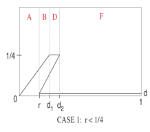
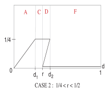
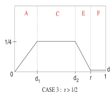
Figure 2: The curve of $\lambda$ given in Theorem 2 depending on $d$.

2.3 The traffic fundamental diagram

The system (8)–(12) admits a growth rate $f=\lim_{k\to+\infty}x^{k}/k$ for trajectories starting from $0$. This quantity has the interpretation of the average car flow (for this reason, we denote it by $f$ rather than $\chi$). It is difficult to obtain an analytical expression for $f$. Nevertheless, it is easy to compute an approximation by numerical simulation. Choosing a $K$ large enough, we have $f\simeq x^{K}/K$. Clearly this quantity depends on the car density and on the car positions at initial time. However, we have remarked by simulation that the dependence with the initial car positions is not very important and disappears when the size of the system (size of the roads and number of cars) increases. Asymptotically, the average car flow depends only on the density $d$ and on the relative sizes of the roads $r$. Moreover, since the system is not monotone, the eigenvalue is not equal to the growth rate (see (Farhi et al., 2009)). However, we see by simulation that the average car flow $f$ is always close to one of the eigenvalues $\lambda$. The left side of Figure 3 shows numerical simulations for different values of $r$. This figure tells that when the eigenvalue is not unique, the average car flow chooses the eigenvalue zero (see also Figure 4 below). In the right side of Figure 3, we see that $\lambda$ and $f$ are very close to each other when $\lambda$ is unique (i.e. when $r>1/2$). This figure tells that $f$ and $\lambda$ differ mainly in one phase among from the four traffic phases (see the traffic phases analysis in section 2.4 below).

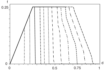
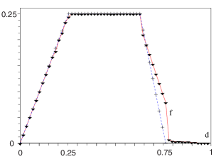
Figure 3: On the left side: The fundamental diagram of 2D-traffic depending on the ratio $r$, where $r$ takes the values: 0.15, 0.20, 0.25, 0.35, 0.40, 0.45, 0.50, 0.60, 0.70, 0.75, 0.85 and 0.95, respectively from the left to the right. On the right side: Comparison of $f$ and $\lambda$ in the case $n=45,m=15$, i.e. $r=3/4>1/2$.

In the left side of Figure 3, we give the dependence of $f$ with $d$ and $r$. For a given $r$, the function $f(d)$ is a generalization to 2D-traffic systems (presence of junctions) of what is called fundamental diagram in traffic literature.

The eigenvalue, when it is unique, gives a good analytical approximation of the average flow. When it is not unique, we have to choose the good one (in this case the eigenvalue 0). Finally, we obtain a good approximation of the flow by the formula :

$$f=\max\left\{\min\left\{d,\;\frac{1}{4},\;\frac{r-d}{\max\{2r-1,\;0\}}\right\},0\right\},$$ (21)

where $a/0=\text{sign}(a)\infty$. Therefore when $r\leq 1/2$ we have $\max\{2r-1,0\}=0$, then, for $d<r$ we obtain $f=\min\{d,1/4\}$ and for $d\geq r$ we obtain $f=0$.

In Figure 4 (to be compared with Figure 2), we give a graphic summary of the different possible cases.

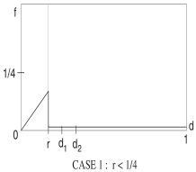
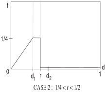
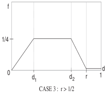
Figure 4: Summary of the fundamental diagrams obtained numerically.

2.4 The traffic phases of the global fundamental diagram

When $r>1/2$ there are four phases. When $r<1/2$ the third phase vanishes, and when $r<1/4$ even the second phase vanishes. Let us discuss the physical interpretation of these four phases.

1. Free phase: $0\leq d\leq d_{1}$.

   In this case, at the stationary regime, the cars are separated by free cells and move freely. There is no effect of the intersection, and the behavior of the system is similar to a simple circular road. The flow is $f=d$.

   

   

   Figure 5: Positions of cars in the free phase: initial and periodic asymptotic. Sizes: $n=40,m=20$. The number of vehicles is $12$.

2. Saturation phase: $d_{1}\leq d\leq d_{2}$.

   This phase appears as soon as $r>1/4$. In this case, the intersection is never free, and its output flow is maximum and equal to $1/4$. Thanks to the priority rule, after an initial transition period, the flow on the priority road is regular, and the density of cars on this road is given by the maximal output flow of the intersection (which is $1/4$). All the other cars are on the non-priority road. $N$ being the total number of cars, $m/4$ cars stay on the priority road and $N-m/4$ stay on the non-priority road. The flow on the non-priority road must be equal to $1/4$ in such a way that the junction be always fed. The non-priority road is seen as a circular road with a retarder (a slow cell), see (Farhi et al., 2005). The role of the retarder is played here by the intersection. Thanks to the works presented in (Farhi et al., 2005), it is understood that the flow $1/4$ is reached when the density belongs to $[1/4,3/4]$ on circular roads with retarder. This last constraint gives $n/4\leq N-m/4\leq 3n/4$, which is obtained when $d_{1}\leq d\leq d_{2}$.

   

   

   Figure 6: Positions of cars in the saturation phase: initial and periodic asymptotic. Sizes: $n=40,m=20$. The number of vehicles is $30$.

3. The recession phase: $d_{2}\leq d\leq r$.

   This phase appears only when the non-priority road is longer than the priority road, that is when $r>1/2$. In this case, this phase appears when the global density exceeds $d_{2}$, that is when the number of vehicles in the system exceeds $m/4+3n/4$. The flow on the non-priority road is less than $1/4$ because the density of vehicles on this road exceeds $3n/4$. The cells immediately downstream from the junction in the non-priority road are crowded, and thus the junction cannot serve with its maximal flow, so the global flow is less than $1/4$. Since the density of vehicles in the priority road is given by the output flow of the junction, this density is less than $1/4$ and it decreases by increasing the global density. So when we increase the global density slowly in this phase, the whole number of added vehicles is added to the non-priority road, and moreover, vehicles on the priority road are pumped onto the non-priority road.

   This phase starts when the density is such that $m/4$ vehicles are in the priority road, and $3n/4$ vehicles are on the non-priority road. Thus, we have $N=m/4+3n/4$, which gives $d=d_{2}$.

   Since this phase is characterized by the pumping of the priority road vehicles, the end of this phase appears when the density is such that no vehicle stays on the priority road. When we have $n$ vehicles on the non priority road its density is $1$. Thus we get $N=n$, which gives $d=r$, thus $d_{2}<d<r.$

   

   

   

   Figure 7: Positions of cars in the recession phase: initial and periodic asymptotic. Sizes: $n=40,m=20$. The number of vehicles is $37$.

4. The freeze phase: $r\leq d\leq 1$.

   When the total number of cars exceeds the size of the non- priority road, a jam appears. In this case, the non-priority road fills up. When a car in the intersection wants to enter this road, the system blocks.

   

   

   Figure 8: Positions of cars in the freeze phase: initial and periodic asymptotic. Sizes: $n=40,m=20$. The number of vehicles is $50$.

2.5 The fundamental diagram of the individual roads

Let us discuss the fundamental diagrams for the two roads. For this we need the densities $d_{m}$ on the priority road and $d_{n}$ on the non-priority road. It is easy to check that:

$$d=rd_{n}+(1-r)d_{m}.$$ (22)

Using (22) we get the diagrams plotted on Figure 9.

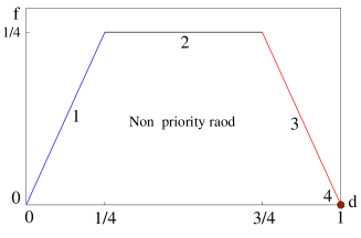
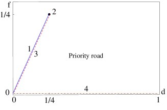
Figure 9: Approximate fundamental diagram on each road. 1: Free phase, 2: Saturation phase, 3: Recession phase, 4: Freeze phase.

1. Free phase: In this phase, we have $d=d_{m}=d_{n}=f$. Thus, the diagrams are $f=d_{m}$ and $f=d_{n}$ with $0\leq d_{m}\leq 1/4$ and $0\leq d_{n}\leq 1/4$.

2. Saturation phase: In this case, the global flow $f$ and the density $d_{m}$ are constant and are equal to $1/4$. Then the diagram of the priority road is restricted to the point $(1/4,1/4)$.

   From (22), we get $d_{n}=d/r-(1-r)/4r,$ then $1/4\leq d_{n}\leq 3/4$ from $d_{1}\leq d\leq d_{2}$. Hence the diagram of the non-priority road is given by the segment $[(1/4,1/4)\;,\;(3/4,1/4)]$.

3. Recession phase: Let us give a simplified description of what happens in this phase. In fact, we see on numerical simulations a more complicated periodic regime where the densities of the car do not stay approximately constant as in the other phases.

   The pumping phenomena makes the density of the priority road low. Thus the vehicles are moving freely on this road. We have $d_{m}=f=(r-d)/(2r-1)$. Then $d_{2}\leq d\leq r$ gives $0\leq d_{m}\leq 1/4$. Therefore, the diagram for the priority road is the segment $[(1/4,1/4)\;,\;(0,0)]$.

   From (22), we get $d_{n}=d/(2r-1)d-(1-r)/(2r-1),$ which must satisfy $3/4<d_{n}<1$ to be crowded enough. That is implied by $d_{2}<d<r$. Moreover, we have $f=1-d_{n}=(r-d)/(2r-1)$ for a road without intersection (see (Farhi et al., 2005)). Therefore, the diagram for the non-priority road is the segment $[(3/4,1/4)\;,\;(1,0)]$.

4. Freeze phase: In this case, we have $d_{n}=1$ and $f=0$, and the diagram of the non-priority road is restricted to the point $(1,0)$. From (22), we get $d_{m}=d/(1-r)-r/(1-r)$. Therefore, $r\leq d\leq 1$ gives $0\leq d_{m}\leq 1$. The diagram for the priority road in this phase is the segment $[(0,0)\;,\;(1,0)]$.

In this study, the turning movement percentage is taken equal to $1/2$, but the same approach can be used to study the general case, where this percentage is a parameter $\alpha$. Preliminary works, show that a function of $r$ and $\alpha$ could play the same role as $r$ here.

3 Extension to more than one junction

In this section, we extend the one junction model to the case with two junctions first, then to a regular city on a torus. We use the same vehicle dynamics and junction management (right priority, turning policy) as in the case of one junction. To be able to fix the car densities, we consider, as in section 2, closed systems. In the case of a city, the simplest way to obtain a closed system is to consider a regular city on a torus; see Figure 19. We show that the shape of the fundamental diagram is mainly the same as in the case of one junction.

3.1 The case of two junctions

We consider a system of two circular roads crossing on two junctions, as shown on Figure 10. This configuration gives four roads without intersections (R1, R2, R3 and R4). The road R2 (resp. R3) has priority over the road R1 (resp. R4).

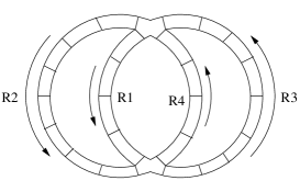
Figure 10: Two circular roads crossing on two junctions.

Using the same approach as in the case of one junction, we can derive easily the dynamics of this system. A systematic way to determine such a kind of model is described in (Farhi, 2008) . Here we will discuss only the fundamental diagram obtained and its phases.

$\bullet$ The first important observation that we can make is that the fundamental diagram depends on the sizes of the four roads only through the ratio between the sum of the priority road sizes and the sum of the non-priority road sizes called $r$; see Figure 11.

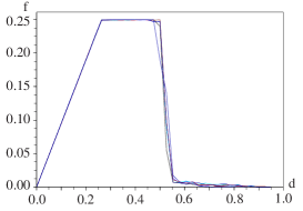
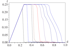
Figure 11: On the left side: the fundamental diagram on the whole system for various sizes of the four roads with $r$ maintained constant: $r=1/2$. On the right side: the fundamental diagram on the whole system for different values of $r$, respectively from the left to the right: $2/10,3/10,4/10,5/10,6/10,7/10,8/10,9/10,9.5/10$.

$\bullet$ The second important observation is that in terms of the fundamental diagram of traffic, a system of four roads with two junctions with a ratio $r$ between the sum of the priority road sizes and the sum of the non-priority road sizes behaves like a system of two roads with one junction with the same ratio $r$ between the size of the priority road and the size of the non-priority road; see Figure 12.

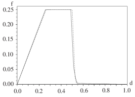
Figure 12: Comparison of the fundamental diagrams for one and two junctions with the same $r=1/2$.

$\bullet$ The third observation is that the traffic phases are similar to those obtained in the case of one junction. Here also, the asymptotic regimes are well understood. Figures (13), (14), (15) and (16) show the stationary regimes corresponding to the four phases.

1. Free phase: After a mixing regime where the cars split on the different roads in equal populations, a periodic regime appears where the vehicles move freely and where the priority rule is never applied; see Figure (13). During the periodic regime, the vehicles are sufficiently separated so as to not disturb each other on the roads or in the intersections. Thus, all the vehicles move every time. That gives the same flow on all the roads, which is equal to the density of vehicles on the network. This phase corresponds to densities from $0$ to $1/4$.

   

   

   Figure 13: Initial and asymptotic periodic configurations during the free phase. The size of each priority road is 10. The size of each non-priority road is 20. The total number of vehicles is 10.

2. Saturation phase: A periodic regime is reached where the junctions serve with their maximal flow applying the priority rule. Thus, the vehicles are accumulated in the non-priority roads; see Figure 14. During the periodic regime, the average number of vehicles moving on the priority roads remains the same as in the case of the density $d=1/4$. This means that all the added vehicles, with respect to the density $1/4$, are absorbed by the non-priority roads. The junctions serve with the maximal flow. Hence, the average flow is equal to $1/4$. The saturation phase is given by a horizontal segment on the global diagram (Figure 11) and on the diagrams corresponding to the non-priority roads (Figure 17, Roads 1 and 4.  Figure 18, left side). The saturation phase is given by a dot on the diagrams corresponding to the priority roads, because the number of vehicles in the priority roads is unchanged (Figure 17, Roads 2 and 3. Figure 18, right side).

   

   

   Figure 14: Initial and asymptotic periodic configurations during the saturation phase. The size of each priority road is 10. The size of each non-priority road is 20. The total number of vehicles is 30.

3. Recession phase: This phase appears only when the sum of the priority road sizes is less than the sum of the non-priority road sizes. In this case, the vehicles continue to be accumulated in the non-priority roads by increasing the density (with respect to the saturation phase). At the periodic regime, the number of vehicles on the non-priority roads is so big that the flow is less than $1/4$, but this number is insufficient to fill up the non-priority roads and freeze the traffic (which corresponds to the freeze phase, see below).

   

   

   

   Figure 15: Initial and asymptotic periodic configurations during the recession phase. The size of each priority road is 10. The size of each non-priority road is 20. The total number of vehicles is 37.

   During this phase, a phenomenon of pumping vehicles from priority roads to non-priority roads is observed. This can be seen on the fundamental diagram of the priority roads where the density of vehicles on these roads decreases when the global density in the whole system is increased (Figure 17, Roads 2 and 3, Figure 18, right side.).

   Since the density of vehicles in the non-priority roads exceeds $3/4$, the global flow is less than $1/4$ (see 1D-traffic phases in (Farhi, 2008; Farhi et al., 2005)). Since the priority roads are served by a flow less than $1/4$ and the output flow of these roads is bounded by the maximum flow of the junctions (which is $1/4$), the density on these roads is equal to the global flow. The global flow is less than $1/4$ and decreases by increasing the global density. Hence, the density on the priority roads decreases when we increase the global density.

4. Freeze phase: A freeze appears as soon as the number of vehicles on the whole system reaches the sum of the sizes of the non-priority roads. In this case, the traffic freeze results from the non-priority roads filling up and blocking the two junctions; see Figure 16.

   

   

   Figure 16: Initial and asymptotic periodic configurations during the freeze phase. The size of each priority road is 10. The size of each non-priority road is 20. The total number of vehicles is 50.

In Figure 17, we give the fundamental diagram for each road.

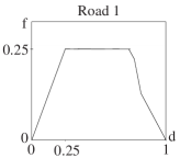
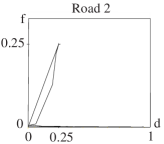
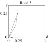
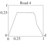
Figure 17: Fundamental diagram on the roads 1, 2, 3 and 4.

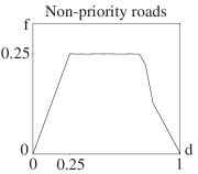
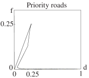
Figure 18: The fundamental diagram of the priority roads (2 and 3) and that of the non priority roads (1 and 4).

3.2 A Regular city on a torus

In this section, we extend the model described in section 2 to the case of a regular city. To fix the density, the city is set on a torus; see Figure 19. We will consider here only the case where all the streets have the same sizes which catch the main qualitative results (that is the presence of mainly four phases). It is not easy to obtain the dynamics of the city but this has been done in a modular way. Details on the construction are available in (Farhi, 2008). From this dynamics, by numerical simulation, we see that the average flow mainly does not depend on the car initial positions, but only on the car density. Therefore the fundamental diagram associated to the city exists empirically. We discuss here these numerical results.

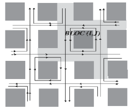
Figure 19: A 4 $\times$ 4 regular city, and a 2 $\times$ 4 regular city on a torus.

As above, we simulate the system for different global densities of vehicles and we derive the traffic fundamental diagram. Numerically we observe the existence of the average flow becoming independent of the initial car distribution when the size of the system grows. As above, numerical diagrams give two, three, or four traffic phases depending on the sizes of the roads. We confirm the observations made in the case of two junctions on the dependence of this diagram on the ratio between the sum of the sizes of the non-priority roads and the sum of the sizes of the priority roads. However, we observed that the beginnings of the recession and of the freeze phases depend also on the lengths of road circuits. Indeed, besides the free density phase where the vehicles move freely, more vehicles circulate on the non-priority roads during the other phases. As soon as the average density of vehicles on a circuit made by non-priority roads exceeds 3/4, the recession phase appears. Similarly, for much higher densities, as soon as a circuit of non-priority roads fills up, the traffic is frozen. However, we think that this dependence of the traffic phases on the lengths of the non-priority road circuits may disappear when the size of the system grows. To confirm or reverse this assumption, we shall extend the analytical results obtained on small systems to larger systems.

In Figure 20, we show the initial and the asymptotic positions of the vehicles in a $4\times 4$ regular city on a torus, for the three phases (free, saturation, and freeze phases) appearing in the symmetric case (where all the roads have the same size, so $r=1/2$, and where the turning percentages are all equal to $1/2$). The traffic behavior during the free and the saturation phases are almost the same as in the case of two junctions. However, the recession and the freeze phases can appear for smaller densities comparing to the case of two junctions. Note that in the case of two junctions only one non-priority road circuit exists, whose length is also the sum of the sizes of all the non-priority roads of the system. In the case of a regular city or a system with more than two junctions, the blocking state can be reached before all the non-priority roads fill up, that is, when the global density $d$ satisfies $d<r$.

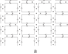
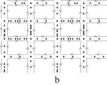
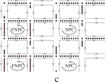
Figure 20: The periodic regime in the cases: (a) free phase ($d=64/304\approx 0.21$), (b) saturation phase ($d=120/304\approx 0.39$), and (c) freeze phase ($d=188/304\approx 0.61$). NPC: non-priority road circuit, FNPC: full non-priority road circuit.

4 Traffic Control

To control the traffic in a regular city, we use traffic lights. We suppose the existence of a traffic light at the exit of each road, which is also an entry to a junction. The traffic lights have only green and red colors with the standard traffic meaning. To construct a regular city controlled by traffic lights, we follow the same approach as in the case of a regular city managed with the priority rule. That is, we develop a model of one junction controlled by a traffic light (see (Farhi, 2008) where we have presented many Petri net models with traffic lights), then we generalize it to a regular city on a torus (see also (Farhi, 2008) where the construction of the controlled regular city is explained.) From the numerical simulation of these models we see that the fundamental diagram makes sense, that is that the car initial position does not hava notable influence on the average flow. The average flow depends only on the car density and on the light strategy. In this section we discuss the different light strategies used and their corresponding fundamental diagrams for a city on a torus.

4.1 Open loop control

In applying an open-loop control, one can consider a periodic traffic plan over time for each junction or a periodic plan for all the network. Here we consider the latter case. First, we fix the period called the cycle. Then we fix the duration of time assigned to the green color and the duration of time assigned to the red color. The timings are chosen with consideration of the traffic on each road, but they are chosen only once and used thereafter.

We test this approach on regular cities where all the roads have the same size, and all the turning proportions are equal to $1/2$. We fix the cycle to 4 units of time. Indeed, since the car flow cannot exceed $1/4$ at the junctions (see subsection 2.1), $4$ units of time is the shortest possible value of the cycle for our model. This cycle time is not realistic but gives the largest flow. The durations of green and red colors are fixed to 2 units of time.

The fundamental diagram obtained with this policy is shown in Figure 22, where we compare it to the other policies described below. For the right priority policy the freeze phase starts at the density $1/2$. Therefore the open-loop control extends the saturation phase and reduces the freeze phase, the free phase being almost unchanged.

4.2 Local feedback control

The local feedback control depends on the state of the traffic on the roads. By local feedback we mean that at every instant and at every junction the control depends only on the traffic on the roads entering the junction and not on the other roads. Let us clarify it. We denote by :

• $R_{1}$ and $R_{2}$ the two roads entering the junction,

• $n_{1}$ and $n_{2}$ their sizes,

• $z_{1}^{k}$ and $z_{2}^{k}$ the number of vehicles on the corresponding road at time $k$,

• $b_{1}^{k}$ and $b_{2}^{k}$ given by $\begin{cases}1&\text{if at time $k$ there is a vehicle intending to enter}\\ &\text{the junction, on the corresponding road,}\\ 0&\text{otherwise.}\end{cases}$

The feedback control $u^{k}$ at time $k$ is given by:

$$u^{k}=\begin{cases}\text{green for }R_{1}\text{ and red for }R_{2}&\text{if }n_{2}b_{1}^{k}+z_{1}^{k}\geq n_{1}b_{2}^{k}+z_{2}^{k},\\ \text{green for }R_{2}\text{ and red for }R_{1}&\hbox{otherwise.}\end{cases}$$

This feedback gives the green color to the road with a vehicle intending to enter the junction when there is only one such a road, and to the more crowded road (relatively to its size) in the other cases. This policy is applied to all the junctions.

The fundamental diagram obtained is given in Figure 22. We can see that the local feedback control is clearly better than the open-loop control since the freeze phase range is reduced to zero without any worsening of the other phases.

In Figure 21, we compare open-loop and feedback traffic controls in terms of the distribution of vehicles at the periodic regime. We see that the local feedback induces a stationary regime where the vehicles are more uniformly distributed (on the roads) comparing to the open loop control case.

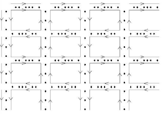
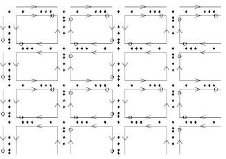
Figure 21: Stationary regimes. On the left side: open loop light control. On the right side: local feedback light control.

The objective in this example is to show the existence of initial car configurations, for which it is better (in terms of car distribution on the city) to manage the traffic by a local feedback control than by an open-loop control.

4.3 Global feedback control

In this section, we follow the point of view developed in TUC (Traffic Urban Control, see (Diakaki et al., 2002)) and use a global feedback based on a linear quadratic stabilization around a nominal trajectory of the traffic in a city. In this modeling, the streets are seen as car inventories flowing from one road to another. We suppose the existence of a traffic light that we can control at each ingoing street of the junctions.

At time $k$ for road $i$ we denote $x_{i}^{k}$ as the number of vehicles, $\bar{x}_{i}$ as the nominal number of vehicles wanted, $u_{i}^{k}$ as the flow outgoing from the road $i$ during the green phase, and $\bar{u}$ as the nominal flow wanted in this road. We solve the linear quadratic control problem :

$$\min_{u\in\mathcal{U}} \sum_{k=0}^{+\infty}(x^{k}-\bar{x})^{\prime}Q(x^{k}-\bar{x})+(u^{k}-\bar{u})^{\prime}R(u^{k}-\bar{u})$$

$$(x^{k+1}-\bar{x})=(x^{k}-\bar{x})+B(u^{k}-\bar{u}).$$ (23)

where $B$ is a matrix describing the interconnections of the streets (each junction has a proportion to enter the outgoing street), and $Q$ and $R$ are weight diagonal matrices that we have to choose empirically to obtain a regulator working in a satisfactory way. The result of this optimization is a global feedback used to determine the timing of the traffic light in the microscopic modeling of the city. The fundamental diagram obtained with this control is given in Figure 22.

4.4 Fundamental diagram comparison of traffic light policies

Figure 22 shows the fundamental diagrams obtained with the four junction policies: – priority to the right rule (diagram 1), – open-loop control (diagram 2), – local feedback control (diagram 3), and – global feedback control (diagram 4). For low densities, the flows are almost the same and are equal to the density. However, during this phase, the open-loop control policy (diagram 2) and the global feedback control policy (diagram 4) slow down slightly the flow with respect to the right policy control (diagram 1) or to the local feedback control policy (diagram 3). In the case of open-loop control policy, this can be explained by the fact that at each junction, a vehicle can be stopped by a traffic light on a road even if there is no vehicle intending to move into the junction from the other road. This fact is also observed in the case of global feedback control. It is due to the implementation constraint of these feedback control policies which impose a minimum green and red time.

The critical density at which the freezing appears in the case of the priority to the right policy is 1/2. This value represents also the ratio between the sum of the sizes of the non-priority roads and the sum of the sizes of the priority roads for a symmetric city. (All the roads have the same size, thus the ratio is equal to 1/2.) All the other policies improve the density at which appear the recession and the freeze phases. The best one is the global feedback.

The maximal flow, obtained in the saturation phase, corresponds to the saturation of the junctions which are all the same in this regular city case.

As it can be easily predicted, the flow obtained for low densities (densities less than $1/4$) and by using any of the policies, is equal to the car density. Indeed, for low densities, the vehicles reach asymptotic regimes where they can move freely, independently of the traffic control policy applied at the junctions. For densities $d$ in $[0,1/2)$, the fundamental diagram is the same for all the control policies. We have understood from simulations that in the case of priority to the right rule, we need to increase considerably the sizes of the roads in order to obtain the value $1/4$ of the flow for a density less than but very close to $1/2$. On the diagram 1 of Figure 22, the maximal density for which we obtained the value $1/4$ of the flow is around $0.4$. It is possible to obtain a maximal density much closer to $1/2$ by increasing the sizes of the roads, but long time would be required to simulate the system.

The result obtained for the feedback control policies is surprising. The global feedback always should be better than the local feedback, but the implementation is different. In the global feedback case, we impose a light cycle that we do not impose for the local feedback case. This is the reason why the local feedback seems better than the global one at the end of the recession phase. Up to this consideration the global feedback is the best strategy. The improvement with respect to the open-loop appears only for high densities. All these remarks are quite natural but we see that the light control –even with the open-loop policy– significantly improves the diagram with respect to the priority to the right managing without large deterioration at low densities.

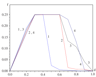
Figure 22: Comparison of traffic control policies on a regular city (set on a torus). 1. Priority rule. 2. Open loop signal light control. 3. Local feedback signal light control. 4. Global feedback signal light control.

4.5 Response time comparison

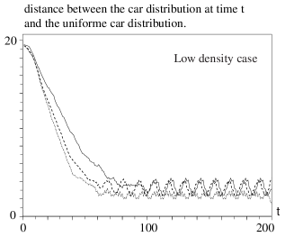
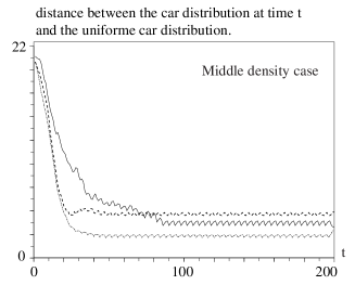
Figure 23: Distance of the vehicle distribution to the uniform distribution as function of time. On the left side: a low density case. On the right side: a middle density case. Continuous line: open loop control. Bold discontinuous line: local feedback control. Alternated discontinuous line: global feedback control.

Figure 23 gives the response times (i.e. time to recover the stationary or periodic regime after a disturbance) obtained for the open-loop, local and global feedback policies. In this figure, we plot the distance between the present vehicle distribution and a uniform car distribution on the streets as a time function. The city has four horizontal and four vertical roads.

Independently from the density, the feedback control gives a better time of response than the open loop control. Both feedback controls are quite similar in terms of time response, but the global feedback asymptotic regime is closer to the uniform distribution.

Remark 3.

A regular city can be closed in different ways. We think that the way the network is closed will not have impact on the qualitative results obtained here. We would have the same traffic phases. In the case where junctions are managed with the priority rule, non priority road circuits would play the same role on the beginning of the freeze phase, independently of the network topology.

5 Junction Design Improvement

As explained above in section 2, the flow is limited by the maximal junction flow which is equal to $1/4$. It is possible to improve the traffic by adding one car place in the junctions. It is easy to check that with this improvement, the bound will be $1/2$ instead of $1/4$.

Let us give the analytical result obtained for the elementary system of one circular road taking shape of the numeral eight (8), with one junction. The only change on the model is on the constraints (13):

$$\begin{cases}0\leq a_{i}\leq 1,\;\;1\leq i\leq n+m\;,\\ 0\leq a_{n}+a_{n+m}\leq 1.\end{cases}\text{ becomes }\begin{cases}0\leq a_{i}\leq 1,\;\;1\leq i\leq n+m\;,\\ 0\leq a_{n}+a_{n+m}\leq 2.\end{cases}$$ (24)

In this new case, we are able to obtain results analogous to Theorem 2 and Corollary 2.

Theorem 3.

There exists an additive eigenvalue $\lambda$ satisfying:

$$0=\max\left\{\min\left\{d-(1+\rho)\lambda,\;r-d-\left(2r-1+\rho\right)\lambda\right\},\;-\lambda\right\}.$$

Corollary 3.

For large values of $n$ and $m$ such that $n>m-2$ (which is the case $r\geq 1/2$), a non negative eigenvalue $\lambda$ is given by:

$$\lambda=\max\left\{\min\left\{d,\;\frac{r-d}{2r-1}\right\},0\right\}.$$

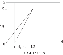
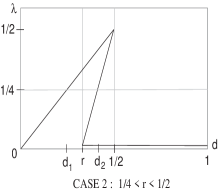
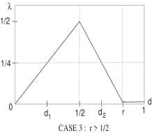
Figure 24: The curve of $\lambda$ given in Theorem 3 depending on $d$, in the case of a large junction.

From this result, we obtain a good approximation of the fundamental diagram :

$$f=\max\left\{\min\left\{d\;,\frac{r-d}{\max\{2r-1,\;0\}}\right\},0\right\},$$ (25)

which is shown in Figure 25.

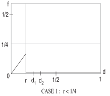
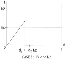
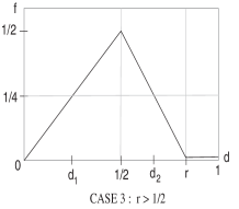
Figure 25: Summary of the fundamental diagrams obtained numerically in the case of a large junction.

6 Conclusion

The main contribution of this paper is the discussion of the phases that can appear in the traffic on a road network. We discuss in detail the four traffic phases (free, saturation, recession and freeze phases) first on elementary systems and then on larger road systems. We identify a key parameter that is a ratio between the sum of the sizes of the non-priority roads and the sum of the sizes of the priority roads. We discuss how the freeze phase appears when a circuit of non-priority road jam is created. On the fundamental diagram, we study the improvement obtained thanks to open loop, local and global feedback traffic light policies. The importance of the junction capacity optimization is revealed clearly by this diagram.

The analytic results are obtained only in the case of two roads with one junction. It would be interesting to analyze the simplest case of two circuits of non-priority roads of different sizes in greater detail to find out if there exists a new phenomenon.

More realistic models should confirm the very natural qualitative results obtained here, but it would be worthwhile to see them on a large set of more sophisticated simulations.

The fundamental diagram should have sense also in the case of open networks for zones of a system where the car density stay almost fixed. The fundamental diagram must be considered, for traffic, as the analogue of the ideal gas law. It should be useful to build 2D fluid macroscopic traffic models based on this law but this possibility has not been explored for the moment.

References

- Biham et al. (1992) Biham, O., Middleton, A. A., Levine, D., 1992. Self-organization and a dynamical transition in traffic flow models. Phys. Rev. A 46.
- Blank (2000) Blank, M., 2000. Variational principles in the analysis of traffic flows. Markov Processes and Related fields 7 (3), pp. 287–305.
- Brockfeld et al. (2001) Brockfeld, E., Barlovic, R., Schadschneider, A., Schreckenberg, M., 2001. Optimizing traffic lights in a cellular automaton model for city traffic. Physical Review E 64 (056132).
- Buisson and Ladier (2009) Buisson, C., Ladier, C., 2009. Exploring the impact of the homogeneity of traffic measurements on the existence of macroscopic fundamental diagrams. In the 88th Transportation Reserarch Board meeting and to appear in Transportation Research Record.
- Chowdhury et al. (2000) Chowdhury, D., Santen, L., Schadschneider, A., 2000. Statistical physics of vehicular traffic and some related systems. Physics Reports (329), 199–329.
- Cuesta et al. (1993) Cuesta, J., Martinez, F., Molera, J., Sanchez, A., 1993. Phase transition in two dimensional traffic-flow models. Physical Review E 48 (6), R4175–R4178.
- Daganzo (2005) Daganzo, C. F., 2005. A variational formulation of kinematic waves: Basic theory and complex boundary conditions. Transportation Research part B 39 (2), 187–196.