Entanglement Entropy as a Portal to the Physics of Quantum Spin Liquids

Abstract

Quantum Spin Liquids (QSLs) are phases of interacting spins that do not order even at the absolute zero temperature, making it impossible to characterize them by a local order parameter. In this article, we review the unique view provided by the quantum entanglement on QSLs. We illustrate the crucial role of Topological Entanglement Entropy in diagnosing the non-local order in QSLs, using specific examples such as the Chiral Spin Liquid. We also demonstrate the detection of anyonic quasiparticles and their braiding statistics using quantum entanglement. In the context of gapless QSLs, we discuss the detection of emergent fermionic spinons in a bosonic wavefunction, by studying the size dependence of entanglement entropy.

I Introduction

Quantum Spin Liquids (QSLs) are phases of strongly interacting spins that do not order even at absolute zero temperature and therefore, are not characterized by a Landau order parameter balentsreview . They are associated with remarkable phenomena such as fractional quantum numbers anderson1973 ; anderson1987 ; baskaran1987 ; read1991 , transmutation of statistics (eg. fermions appearing in a purely bosonic model)kivelson1987 ; read1989 , and enabling otherwise impossible quantum phase transitionssenthil2004 , to name a few. Spin liquids may be gapless or gapped. While current experimental candidates for spin liquids appear to have gapless excitations exp , gapped spin liquids are indicated in numerical studies on the Kagome yan2010 ; hongchen2012 , square Balents ; Wen and honeycomb lattice meng2010 . A distinctive property of gapped spin liquids is that they are characterized by topological order - i.e. ground state degeneracy that depends on the topology of the underlying spacewen2004 ; hastings2004 . The gapless spin liquids are relatively difficult to characterize and their low-energy description often involves strongly interacting matter-gauge theories mattergauge .

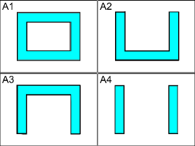
Figure 1: Following Ref. levin2006, , consider four regions $A_{1}$-$A_{4}$ (shaded cyan). The thickness as well as the linear size of all regions $A_{i}$ is much bigger than the correlation length $\xi$ of the system. The combination $(S_{1}-S_{2})-(S_{3}-S_{4})$ equals zero for short-range entangled systems. To see this, we note that $S_{1}-S_{2}$ and $S_{3}-S_{4}$ correspond to the change in entanglement entropy associated with closing the region $A_{2}$ and $A_{4}$, respectively, at the top. For a wavefunction with short-range entanglement, the difference $(S_{1}-S_{2})-(S_{3}-S_{4})$ should vanish as $e^{-R/\xi}$ where $R$ is approximately the linear size of regions $A_{i}$. Therefore, a non-zero $\gamma$ implies that the system is long-range entangled.

In the theoretical search for QSLs, two qualitatively different kinds of questions can be asked:

• Given a particular Hamiltonian $H$, does it admit a QSL as its ground-state? If yes, can one further characterize the QSL?

• Given a ground state wavefunction(s), can one tell if it corresponds to a QSL? If yes, can one further characterize the QSL?

These two questions are related: if a numerical scheme can provide one with access to approximate ground state wavefunction of a particular Hamiltonian $H$, then answering the second question leads to an answer to the first one as well. The recent years have seen remarkable progress in tackling these questions. Of particular usefulness has been the application of ideas from quantum information science to quantum many-body physics. Motivated by these developments, in this review we will focus on the second question above from an information theoretic point of view, and we will discuss some of the advances on the first question in the section VII.

The usefulness of entanglement entropy to understand the physics of QSLs becomes apparent when one introduces the notion of ‘short-range’ and ‘long-range’ entanglement. The heuristic picture of a short-range entangled phase is that its caricature ground state wavefunction can be written as a direct product state in the real space, hence the nomenclature. The phases of matter that do not satisfy this property are thereby called ‘long-range entangled’. From this definition, gapless phases, such as a Fermi liquid or superfluid, that exhibit algebraic decay of local operators are always long-range entangled in the real space. Naively, one might think that the converse would hold, that is, existence of short-range correlations for local operators will imply short-range correlation. It is precisely here that the connection between gapped QSLs and ground state entanglement properties comes into play. To wit, gapped QSLs are phases of matter that show long-range entanglement in their ground states despite the fact that the correlation functions of all local operators decay exponentially with distance.

To make the connection between gapped QSLs and long-range entanglement precise, let us define some basic terminology that will also be useful throughout this review. Given a normalized wavefunction, $|\phi\rangle$, and a partition of the system into subsystems $A$ and $B$, one can trace out the subsystem B to give a density matrix on A: $\rho_{A}={\rm Tr}_{B}|\phi\rangle\langle\phi|$. The Renyi entropies are defined by:

$$S_{n}=\frac{1}{1-n}\log({\rm Tr}\rho_{A}^{n})$$ (1)

It is common to pay special attention to the von Neumann entropy, $S_{1}=-{\rm Tr}[\rho_{A}\log\rho_{A}]$ (obtained by taking the limit $n\rightarrow 1$ in Eqn.1). However, the Renyi entropies are also equally good measures of entanglement, and are often easier to compute.

In seminal papers by Kitaev, Preskill kitaev2006 and Levin, Wen levin2006 , it was shown that the entanglement entropy of a topologically ordered phase, such as a gapped QSL, as a function of the linear size of disc-shaped region $A$ of linear size $l$, receives a universal subleading contribution:

$$S(L)=\frac{l}{a}-b_{0}\gamma+O(1/l)$$ (2)

where $b_{0}$ is the number of connected components of the boundary of region $A$ and the constant $\gamma$ is a universal property of the phase of matter that is non-zero if and only if the phase is topologically ordered. One may wonder why does a non-zero $\gamma$ implies long-range entanglement? One way to understand this levin2006 is to consider the combination $S_{0}=(S_{1}-S_{2})-(S_{3}-S_{4})$ for the geometry shown in Fig.1. If the phase was in fact short-range entangled, then $S_{0}$ will vanish identically. From Eqn.2, $S_{0}=-2\gamma$ and therefore, a non-zero $\gamma$ implies long-range entanglement. A different way to derive the same conclusion is to define a quantity $S_{local}$ such that it is obtained by locally patching the contributions to the entanglement entropy from the boundary $\partial A$ of region $A$ grov2011 . If the phase is short-range entangled, then $S_{local}$ is the entire $S$. As shown in Ref. grov2011, , on general grounds, $S_{local}$ cannot contain a constant term, and therefore, $\gamma\neq 0$ implies long-range entanglement.

Gapless spin-liquids pose a different set of questions. The gapless excitations make it difficult to assign them a simple topological number such as $\gamma$ above. One exception is gapless spin-liquids where the emergent gauge degrees of freedom are gapped and are coupled to gapless matter. In this case, there are known contributions to the entanglement entropy that can characterize the nature of QSL senthilswingle ; pufu . In this review, we will focus on cases where the emergent gauge fields are instead gapless. As an example, consider a two-dimensional QSL where the gapless matter fields are neutral fermions which form a Fermi surface, and are coupled to a gapless gauge field. As we discuss in Sec.VI, empirically one finds that their entanglement entropy scales as $S\sim l\log l$, akin to gapless fermions in two dimensions gioev2006 ; wolf , thus suggesting the presence of emergent fermions in a purely bosonic state.

II Entanglement Entropy and Many Body Physics

One of the most interesting properties of EE is that $S(A)=S(\overline{A})$ where $\overline{A}$ is the complement of region $A$. This suggests that EE is a property of the boundary $\partial A$ of region $A$ since $\partial A=\partial\overline{A}$, which further suggests that for a short-ranged correlated system, EE scales linearly with the the boundary $\partial A$: $S(l)\sim l^{d-1}$ where $l$ is the linear size of region $A$ bombelli ; srednicki . Such a scaling of EE goes by the nomenclature of “Area Law” or “Boundary Law”. Indeed, for one-dimensional systems with a gap, this statement can be proved rigorously hastingsproof and it has also been observed numerically for various gapped two-dimensional systems eisert2010 . Furthermore, even when the correlations of local operators are long-ranged, for example, in a free fermionic system with a Fermi surface, the Boundary Law is violated by only by a multiplicative logarithm, that is, $S(l)\sim l^{d-1}\log(l)$ gioev2006 ; wolf , while for a conformal field theory (CFT), where the low-lying modes exist at only discrete point(s) in the momentum space, the Boundary Law is not violated at all in $d>1$ ryu2006 .

To give a flavor of the information theoretic approach to many-body physics, let us consider one of the earliest such applications that concerns the relation between the central charge $c$ of a one-dimensional CFT, and the coefficient of the logarithmic term in the bipartite entanglement entropy $S$ for the corresponding CFT cftwork . The result is

$$S(l)=\frac{c}{6}\log(\frac{l}{a})$$ (3)

where $l$ is the size of the subsystem $A$ and $a$ is a microscopic cutoff. The main observation to gather from this equation is that just given the ground state wavefunction of a CFT, its central charge can be extracted by calculating the entanglement entropy. Note that rescaling $l\rightarrow l/\alpha$ where $\alpha$ is a non-universal number does not change the coefficient of the logarithm. This makes physical sense, since $c$ is a property of the low-energy theory and should be insensitive to the details of how the theory is regularized at the level of the lattice.

An extension of this result to a two dimensional CFT is ryu2006 :

$$S(l)=\frac{l}{a}-\Gamma$$ (4)

for a region $A$ with linear size $l$ and smooth boundaries. Here $\Gamma$ is a constant that depends only on the shape of region $A$. Rescaling $l\rightarrow l/\alpha$ does not change $\Gamma$ akin to the case of one-dimensional CFT, albeit in this case $\Gamma$ will generically be shape dependent. As we will see, this result will be useful to characterize gapless QSLs whose low-energy theory is a CFT (Sec.VI).

The common feature of the above two examples is that EE as a function of system size $l$ contains terms that are universal properties of the low-energy description of the system. Returning to our topic of interest, namely QSLs, one of the most interesting result kitaev2006 ; levin2006 is that for gapped systems in two dimensions, the subleading term in EE is universal and contains information regarding the presence or absence of topological order, and also partially characterizes the topological order:

$$S(l)=\frac{l}{a}-\gamma+O(1/l)$$ (5)

The subleading constant $\gamma$ is called “Topological Entanglement Entropy” (TEE) and as already mentioned in the introduction, is a universal property of the phase of the matter, even though one happens to have has access to only one of the ground states in the whole phase diagram. $\gamma$ is non-zero if and only if the system has topological order. Furthermore, $\gamma=\log(D)$ where $D=\sqrt{\sum_{i}d^{2}_{i}}$ is the so-called total quantum dimension associated with the phase of matter whose quasiparticles carry a label $d_{i}$, the individual quantum dimension for the $i$’th quasiparticle. As a concrete example, for Kitaev’s Toric code model kitaev2003 , there are four quasiparticles, the identity particle $\mathbf{1}$, the electric charge $\mathbf{e}$, the magnetic charge $\mathbf{m}$, and the dyon $\mathbf{em}$. The quantum dimension is one for each of these quasiparticles and hence the total quantum dimension $D=\sqrt{4}=2$. We note that the the universal contribution to EE was first observed in the context of discrete gauge theories in Ref. hamma2005, .

The Eqn.5 serves as a definitive test to see if a particular ground state corresponds to topological ordered state or not. If the answer is indeed in affirmative and if the state also possesses a global $SU(2)$ spin-rotation symmetry, then it is a gapped QSL. Having established that the wavefunction corresponds to QSL, it is imperative to further characterize the state further since the total quantum dimension $D$ only a partial characterization of topological order. For example, for $D=2$, there exist two distinct QSLs, the $Z_{2}$ QSL, which has the same topological order as the Kitaev’s Toric code kitaev2003 , and the doubled semionic theory levin2005 , which can be thought of as a composite of Laughlin $\nu=1/2$ quantum Hall state and its time-reversed partner. To achieve a detailed characterization of topological order, TEE again turns out to be a very useful concept. As we will show in Sec.V.2.1, TEE can be used to extract not only the individual quantum dimensions $d_{i}$ for the quasiparticles, but there braiding statistics as well.

An elegant different approach to a more complete identification of topological order is through the study of the entanglement spectrum HaldaneLi . This method is extremely useful for phases that have a gapless boundary such as quantum Hall and topological insulators/superconductors, though it may not be applicable for topological phases such as the $Z_{2}$ spin liquid that do not have edge states.

III Variational Wavefunctions for Quantum Spin Liquids

A quantum spin liquid (QSL) can be viewed as a state where each spin forms a singlet with a near neighbor, but the arrangement of singlets fluctuates quantum mechanically so it is a liquid of singlets anderson1973 ; balentsreview . Theoretical models of this singlet liquid fall roughly into two categories. In the first, the singlets are represented as microscopic variables as in quantum dimer and related modelsrokhsar1988 ; moessner2001 ; senthil2002 ; balents2002 ; misguich , and are suggested by large N calculations read1991 . Topological order can then be established by a variety of techniques including exact solutions. In contrast there has been less progress establishing topological order in the second category, which are SU(2) symmetric spin systems where valence bonds are emergent degrees of freedom. More than two decades ago, Andersonanderson1987 proposed constructing an SU(2) symmetric spin liquid wavefunction by starting with a BCS state, derived from the mean field Hamiltonian:

$$H=-\sum_{rr^{\prime}}\{t_{rr^{\prime}}f^{\dagger}_{\sigma,r}f_{\sigma,r^{\prime}}+\Delta_{rr^{\prime}}f^{\dagger}_{\uparrow,r}f^{\dagger}_{\downarrow,r^{\prime}}\}+h.c.$$ (6)

and Gutzwiller projecting gutzwiller1963 it so that there is exactly one fermion per site, hence a spin wavefunction. Variants of these are known to be good variational ground states for local spin Hamiltonians (see e.g. motrunich05 ; varstudy ) and serve as a compact description of most experimental and $SU(2)$ symmetric liquids. Approximate analytical treatments of projection, that include small fluctuations about the above mean field state, indicate that at least two kinds of gapped spin liquids can arise: chiral spin liquidskalmeyer (CSL) and $Z_{2}$ read1991 ; wen1991 ; senthil2000 spin liquids. The low energy theory of CSL corresponds to a Chern-Simons theory while in the $Z_{2}$ spin-liquid, it corresponds to deconfined phase of the $Z_{2}$ gauge theory. However, given the drastic nature of projection, it is unclear if the actual wavefunctions obtained from this procedure are in the same phase as the ground state of a Chern-Simons theory/$Z_{2}$ gauge theory. In fact, detecting deconfinement in a gauge theory in the presence of matter-field is considered notoriously hard fradkinshenker . As we will see below, quantum entanglement provides an elegant solution to this problem.

In contrast to gapped QSLs, the low-energy description of gapless QSLs consist of strongly interacting matter-gauge theories which are harder to analyze mattergauge . Remarkably, the above procedure of constructing mean-field spin-liquid states and using Gutzwiller projection to obtain wavefunctions can be applied to obtain gapless QSLs as well. To do so, one sets the BCS gap $\Delta_{rr^{\prime}}$ in Eqn.6 to zero. This Gutzwiller projection technique is known to work well in one dimension where the projected Fermi sea spin wavefunction captures long distance properties of the Heisenberg chain, and is even known to be the exact ground state of the Haldane-Shastry HaldaneSastry Hamiltonian. Though similar rigorous results are not available in two dimension, a critical spin liquid, the spinon Fermi sea (SFS) state, has been invoked motrunich05 ; palee2005 to account for the intriguing phenomenology of aforementioned triangular lattice organic compounds yamashita2010 . In the SFS state, the spinons $f$ hop on the triangular lattice sites giving rise to a Fermi sea, while strongly interacting with an emergent ‘electromagnetic’ $U(1)$ gauge field. The metal like specific heat and thermal conductivity seen in these materials is potentially an indication of the spinon Fermi surface. In this regard, the Gutzwiller projected Fermi sea is known to have excellent variational energy for the $J_{2}-J_{4}$ spin model on the triangular lattice, which is believed to be appropriate for the aforementioned triangular lattice compoundsmotrunich05 .

As mentioned in the introduction, the main task of this review is to illustrate the extraction of the universal properties of a QSL from the ground state wavefunction. Therefore, we now turn to the technical challenge of calculating EE of Gutzwiller projected wavefunctions that are candidates for QSL.

IV From QSL Wavefunctions to Entanglement Entropy

In this section, using a Monte Carlo scheme, we outline how to obtain the entanglement entropy of a ground state function that has the form of a Gutzwiller projected Slater determinant. As mentioned in the previous sections, such wavefunctions are a natural candidate for QSLs. We will focus on the second Renyi entropy $S_{2}$ (see Eqn. 1) since it suffices to establish topological order and is easiest to calculate within our scheme.

Let $\phi(a,b)$ be the wavefunction of interest, where $a$ ($b$) be the configuration of subsystem A (B). Then the reduced density matrix is $\rho_{A}(a,a^{\prime})=\sum_{b}\phi^{*}(a,b)\phi(a^{\prime},b)/N$ where the normalization $N=\sum_{a,b}\phi^{*}(a,b)\phi(a,b)$. The second Renyi entropy $S_{2}$ is:

$$e^{-S_{2}} = {\rm tr}\rho_{A}^{2}$$ (7)

$$= \frac{1}{N^{2}}\sum_{aa^{\prime}bb^{\prime}}\phi^{*}(a,b)\phi(a^{\prime},b)\phi^{*}(a^{\prime},b^{\prime})\phi(a,b^{\prime})$$

One way to interpret this expression is to consider two copies of the system, in configuration $|a,b\rangle|a^{\prime},b^{\prime}\rangle$. Then, the product wavefunction $|\Phi\rangle=\sum_{a,b,a^{\prime},b^{\prime}}\phi(a,b)\phi(a^{\prime},b^{\prime})|a,b\rangle|a^{\prime},b^{\prime}\rangle$ appears in the expression above. In addition if we define the ${Swap}_{A}$ operator, following Ref hastings2010 , which swaps the configurations of the $A$ subsystem in the two copies:${Swap}_{A}|a,b\rangle|a^{\prime},b^{\prime}\rangle=|a^{\prime},b\rangle|a,b^{\prime}\rangle$ then Renyi entropy can be written simply as:

$$e^{-S_{2}}=\frac{\langle\Phi|{Swap}_{A}|\Phi\rangle}{\langle\Phi|\Phi\rangle}$$ (8)

The above expression suggests a Variational Monte Carlo algorithm for the Renyi Entropy.

Defining configurations $\alpha_{1}=a,\,b$, $\alpha_{2}=a^{\prime},\,b^{\prime}$ and $\beta_{1}=a^{\prime},\,b$, $\beta_{2}=a,\,b^{\prime}$, and $\phi_{\alpha_{1}}=\phi(a,b)$ etc., Eqn.(8) can be rewritten in the suggestive form:

$$\left\langle Swap_{A}\right\rangle=\underset{\alpha_{1}\alpha_{2}}{\sum}\rho_{\alpha_{1}}\rho_{\alpha_{2}}f\left(\alpha_{1},\alpha_{2}\right)$$ (9)

Here the weights $\rho_{\alpha_{i}}=|\phi_{\alpha_{i}}|^{2}/{\sum_{\alpha_{i}}|\phi_{\alpha_{i}}|^{2}}$ are non-negative and normalized. The quantity $f\left(\alpha_{1},\alpha_{2}\right)=\frac{\phi_{\beta_{1}}\phi_{\beta_{2}}}{\phi_{\alpha_{1}}\phi_{\alpha_{2}}}$ when averaged over Markov chains generated with the probability distribution $\rho(\alpha_{1})\,\rho(\alpha_{2})$ yields $\left\langle Swap_{A}\right\rangle$. The Gutzwiller projected wavefunctions to describe the QSLs we consider in this review can be written as products of determinants, as explained in the previous section. Such wavefunctions can be efficiently evaluated, which forms the basis for Variational Monte Carlo technique gros1989 .

As shown in Ref. frank2011crit, ; frank2011topo, , the above algorithm, with slight modifications that we will discuss briefly in Sec.VI, can be used to calculate $S_{2}$ within a few percent of error bar for subsystems with linear size $L_{A}\lesssim 10$, embedded in systems with linear size $L\lesssim 20$.

V Gapped QSLs and Entanglement

Model systems such as Toric code hamma2005 and quantum dimer models furukawa2007 provide a testing ground for the validity of Eqn.5. More realistic interacting quantum systems pose a greater challenge since the analytical methods are limited. Some of the earlier numerical work to extract TEE included exact diagonalization studies on small systems, looking at quantum Hall Laughlin states haque2007 and perturbed Kitaev toric code models hamma2008 . In the context of QSLs, a recent quantum Monte Carlo study isakov2011 on a sign problem free Hamiltonian used TEE to detect $Z_{2}$ topological order. This was a positive definite wave-function, with U(1) rather than SU(2) spin symmetry. In the rest of this section, we will focus on $SU(2)$ symmetric spin-liquids frank2011topo , using the technique explained in the previous section.

V.1 Establishing Topological Order in Gapped QSLs

In this subsection we discuss few examples where using the algorithm to calculate the entanglement entropy discussed in the previous section, one can establish topological order in $SU(2)$ symmetric QSLs frank2011topo . As a first example, let us consider an $SU(2)$ symmetric lattice wavefunction, the Kalmeyer-Laughlin Chiral Spin Liquid (CSL).

State	Expected $\gamma$	$\gamma_{\rm calculated}/\gamma_{\rm expected}$
Unprojected ($\nu=1$)	0	-0.0008$\pm$ 0.0059 ∗
Chiral SL LA=3	$\log\sqrt{2}$	0.99 $\pm$ 0.03
Chiral SL LA=4	$\log\sqrt{2}$	0.99 $\pm$ 0.12
Lattice $\nu=1/3$	$\log\sqrt{3}$	1.07$\pm$ 0.05
Lattice $\nu=1/4$	$\log\sqrt{4}$	1.06 $\pm$ 0.11

Table 1: Topological Entanglement Entropy $\gamma_{\textrm{calculated}}$ of spin-liquid states obtained using Monte Carlo technique discussed in the main text. $\gamma_{\textrm{expected}}$ is the exact value expected in the limit $\xi/l\rightarrow 0$ where $\xi$ is the correlation length and $l$ is the subsystem size.

The Chiral SL is a spin SU(2) singlet ground state, that breaks time reversal and parity symmetrykalmeyer ; thomale . A wavefunction in this phase wave function may be obtained using the slave-particle formalism by Gutzwiller projecting a $d+id$ BCS state kalmeyer . Alternately, it can be obtained by Gutzwiller projection of a hopping model on the square lattice. This model has fermions hopping on the square lattice with a $\pi$ flux through every plaquette and imaginary hoppings across the square lattice diagonals:

$$H=\underset{\left\langle ij\right\rangle}{\sum}t_{ij}f_{i}^{\dagger}f_{j}+i\underset{\left\langle\left\langle ik\right\rangle\right\rangle}{\sum}\Delta_{ik}f_{i}^{\dagger}f_{k}$$ (10)

Here $i$ and $j$ are nearest neighbors and the hopping amplitude $t_{ij}$ is $t$ along the $\hat{y}$ direction and alternating between $t$ and $-t$ in the $\hat{x}$ direction from row to row; and $i$ and $k$ are second nearest neighbors connected by hoppings along the square lattice diagonals, with amplitude $\Delta_{ik}=i\Delta$ along the arrows and $\Delta_{ik}=-i\Delta$ against the arrows, see Fig. 1. The unit cell contains two sublattices $A$ and $B$. This model leads to a gapped state at half filling and the resulting valence band has unit Chern number. This hopping model is equivalent to a $d+id$ BCS state by an $SU\left(2\right)$ Gauge transformationludwig1994 . We use periodic boundary conditions throughout this section.

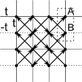
Figure 2: Illustration of a square lattice hopping model connected with a $d+id$ superconductor. While the nearest neighbor hopping is along the square edges with amplitude $t$ ($-t$ for hopping along dashed lines), the second nearest neighbor hopping is along the square diagonal (arrows in bold), with amplitude $+i\Delta$ ($-i\Delta$) when hopping direction is along (against) the arrow. The two sublattices in the unit cell are marked as $A$ and $B$.

Due to the fact that this Hamiltonian contains only real bipartite hoppings and imaginary hoppings between the same sublattices and preserves the particle-hole symmetry, this wavefunction $\left\langle\alpha|\Phi\right\rangle$ can be written as a product of two Slater determinants $\mathcal{M}Det(M_{ij})^{2}$, where $\mathcal{M}$ is just an unimportant Marshall sign factor, and:

$$M_{ij} = \left\{\left[\psi_{A}(k_{i})+\psi_{B}(k_{i})\right]\right.$$ (11)

$$\left.+(-1)^{y_{j}}\left[\psi_{A}(k_{i})-\psi_{B}(k_{i})\right]\right\}e^{ik_{i}\cdot r_{j}}$$

Here $\psi_{A}(k)$($\psi_{B}(k)$) is the wavefunction amplitude on sublattice A(B), $r_{j}$ is the coordinates of the up spins in configuration $\alpha$, and $k_{i}$ is the momentums in the momentum space. The Renyi entropy $S_{2}$ of this wavefunction can be calculated by VMC method detailed in the last section.

Since TEE $\gamma$ is a subleading term in EE, naively it is rather difficult to extract since the leading boundary law term dominates the total entropy. However, as shown by Kitaev and Preskill kitaev2006 , one can divide the total system into four regions $A,B,C,D$ and consider the following linear combination of entropies that completely cancels out the leading non-universal term:

$$-\gamma = S_{2,A}+S_{2,B}+S_{2,C}-S_{2,AB}-S_{2,AC}-S_{2,BC}+$$ (12)

$$S_{2,ABC}$$

where $S_{2,\cal{R}}$ is the Renyi entropy $S_{2}$ corresponding to the region $\cal{R}$. Note that the above formula neglects terms of $O(e^{-\frac{l^{\prime}}{\xi}})$ where $\xi$ is the correlation length and $l^{\prime}=\textrm{min}(l_{A},l_{B},l_{C})$. This is because the above combination of entropies cancels out all local contributions to the entanglement entropy which are expected to form a taylor series expansion in the variable $\xi/l^{\prime}$, following the arguments in Ref.grov2011 . One could still have terms that are non-perturbative in $\xi/l^{\prime}$ which do not cancel out, hence the exponential dependence of the error made. This has also been confirmed by a direct calculation on select models in Ref.fradkin_raman . Therefore, to accurately determine TEE $\gamma$, it is important that $\xi\ll l^{\prime}$. Since we have a variational parameter $\Delta/t$ ar our disposal, one may tune it to minimze the correlation length $\xi$. Chosing an optimal value $\Delta=0.5t$, and dividing the total system with dimensions 12 $\times$ 12 lattice spacings into $L_{A}\times L_{A}$ squares A and B, and an $L_{A}\times 2L_{A}$ rectangle C (see Fig 3), one finds $\gamma=0.343\pm 0.012$ for an $L_{A}=3$ system and $\gamma=0.344\pm 0.043$ for an $L_{A}=4$ system frank2011topo . Both are in excellent consistence with the expectation of $\gamma=\log\left(\sqrt{2}\right)=0.347$ for its ground states’ two fold degeneracy.

To confirm the role of Gutzwiller projection in obtaining the QSL, one may also study the BCS wavefunction used to obtain CSL without Gutzwiller projection. This is an exactly solvable problem and one indeed finds a value $\approx 0$ for TEE. This also serves as a benchmark for the VMC calculation. For an $L_{A}=3$ system, the VMC calculation gives $\gamma=-0.0008\pm 0.0059$, in agreement with vanishing TEE frank2011topo .

One may also study the effect of increasing correlation length on the TEE results. As mentioned above, as correlation length increases, he finite size effects from subleading terms become more important. Indeed, as seen in Fig.4, the TEE calculated using VMC deviates monotonically from the from the universal value of $\gamma=\log\left(\sqrt{2}\right)$ as we lower the gap size $\Delta/t$ for a system with typical length scale $L_{A}=3$.

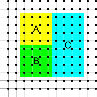
Figure 3: The separation of the system into subsystem $A$, $B$, $C$ and environment, periodic boundary condition is employed in both $\hat{x}$ and $\hat{y}$ directions.

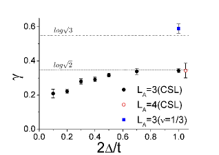
Figure 4: Illustration of finite size effect: chiral SL TEE $\gamma$ as a function of the relative gap size given by $2\Delta/t$ for characteristic system length $L_{A}=3$. The larger the relative gap, the closer the ideal value is approached. For comparison, $\gamma$ for chiral SL at $L_{A}=4$, and a large relative gap, is also shown. On the same plot, TEE of a lattice version of $\nu=1/3$ Laughlin state at $L_{A}=3$, $2\Delta/t=1.0$ is also shown. The dashed lines are the ideal TEE values of $\gamma=\log\left(\sqrt{2}\right)$ for the chiral SL and $\log\left(\sqrt{3}\right)$ for the $\nu=1/3$ Laughlin state.

As mentioned above, the CSL ground state can be written $\sim Det(M_{ij})^{2}$ where $M_{ij}$ is the Slater determinant corresponding to a Chern insulator. This leads to generalization to wavefunctions that are cube or the fourth power of a Chern insulator wavefunction. For example, consider the wavefunction:

$$\Psi_{1/3}(r_{1},\,r_{2}\dots,\,r_{N})=\Phi^{3}(r_{1},\dots,\,r_{N})$$ (13)

where $\Phi$ is the Chern insulator Slater determinant defined above. Clearly, the product is a fermionic wavefunction, since exchanging a pair of particles leads to a change of sign. This is similar in spirit to constructing the corresponding Laughlin liquid of $m=3$ of fermions, by taking the cube of the Slater determinant wavefunction in the lowest Landau level

$$\psi(z_{1},\dots,\,z_{N})=\prod_{i<j}(z_{i}-z_{j})e^{-\sum_{i}\frac{|z_{i}|^{2}}{4l^{2}_{B}}}$$ (14)

However, unlike the canonical Laughlin state, composed of lowest Landau level states, these are lattice wavefunctions. An interesting question is whether the lowest Landau level structure is important in constructing states with the topological order of the Laughlin state, or whether bands with identical Chern number is sufficient, as suggested by field theoretic arguments.

Calculating the TEE using VMC with $L_{A}=3$ one finds $\gamma=0.5894\pm 0.0272$ for the $m=3$ wavefunction, consistent with the ideal value $\gamma=\log\left(\sqrt{3}\right)=0.549$. Similarly, for the fourth power of the Chern insulator Slater determinant, one finds $\gamma=0.732\pm 0.076$, again consistent with ideal value in the thermodynamic limit: $\gamma=\log\left(\sqrt{4}\right)=0.693$.

These results offer direct support for the TEE formula $\gamma=\log D$ as well as their validity as topological ground state wavefunctions carrying fractional charge and statistics. The lattice fractional Quantum Hall wavefunctions discussed here may be relevant to the recent studies of flat band Hamiltonians with fractional quantum Hall states tang2010 ; neupert2010 ; sun2010 ; sheng2011 .

V.2 Beyond TEE: Extracting Quasiparticle Statistics Using Entanglement

At the fundamental level, topologically ordered phases in two dimensions display a number of unique properties such as nontrivial statistics of emergent excitations. For example, in Abelian topological phases, exchange of identical excitations or taking one excitation around another (braiding) leads to characteristic phase factors, which implies that these excitations are neither bosonic nor fermionic. A further remarkable generalization of statistics occurs in non-Abelian phases where excitations introduce a degeneracy. An important and interesting question is whether the ground state directly encodes this information, and if so how one may access it? It is well known that topologically ordered phases feature a ground state degeneracy that depends on the topology of the space on which they are defined. Also, as discussed in the previous sections, the ground state wavefunctions of such states contain a topological contribution to the quantum entanglement, the topological entanglement entropy (TEE). In this section we show that combined together, these two ground state properties can be used to extract the generalized statistics associated with excitations in these states.

The generalized statistics of quasiparticles is formally captured by the modular $\mathcal{S}$ and $\mathcal{U}$ matrices, in both Abelian and non-Abelian states wen1990 ; wen93 ; kitaev_honey ; nayak ; yellowbook . The element $\mathcal{S}_{ij}$ of the modular $\mathcal{S}$ matrix determines the mutual statistics of $i$’th quasiparticle with respect to the $j$’th quasiparticle while the element $\mathcal{U}_{ii}$ of (diagonal) $\mathcal{U}$ matrix determines the self-statistics (‘topological spin’) of the $i$’th quasiparticle. Note, these provide a nearly complete description of a topologically ordered phase - for instance, fusion rules that dictate the outcome of bringing together a pair of quasiparticles, are determined from the modular $\mathcal{S}$ matrix, by the Verlinde formulaVerlinde . Previously, Wen proposed wen1990 using the non-Abelian Berry phase to extract statistics of quasiparticles. However, the idea in Ref. wen1990, requires one to have access to an infinite set of ground-states labeled by a continuous parameter, and is difficult to implement. Recently, Bais et al. Bais also discussed extracting $\mathcal{S}$ matrix in numerical simulations, by explicit braiding of excitations. In contrast, here we will just use the set of ground states on a torus, to determine the braiding and fusing of gapped excitations.

It is sometimes stated without qualification, that TEE is a quantity solely determined by the total quantum dimension $D$ of the underlying topological theory. However, this holds true only when the boundary of the region $A$ consists of topologically trivial closed loops. If the boundary of region $A$ is non-contractible, for example if one divides the torus into a pair of cylinders, generically the entanglement entropy is different for different ground states (see Figure 5). Indeed as shown in Ref. dong2008, for a class of topological states, the TEE depends on the particular linear combination of the ground states when the boundary of region $A$ contains non-contractible loops. We will exploit this dependence to extract information about the topological phase beyond the total quantum dimension $D$.

Let us briefly summarize the key ideas involved in extracting braiding statistics using quantum entanglement frank2012 and then discuss the details. We recall that the number of ground states $N$ on a torus corresponds to the number of distinct quasiparticle types wen1990 ; wen1991 ; footnote_gsd . Intuitively, different ground states are generated by inserting appropriate fluxes ‘inside’ the cycle of the torus, which is only detected by loops circling the torus. We would like to express these quasiparticle states as a linear combination of ground states. A critical insight is that this can be done using the topological entanglement entropy for a region $A$ that wraps around the relevant cycle of the torus. To achieve this, we introduce the notion of minimum entropy states (MESs) $\Xi_{j}$, $j=1-N$, namely the ground states with minimal entanglement entropy (or maximal TEE, since the TEE always reduces the entropy) for a given bipartition. These states are generated by insertion of a definite quasi-particle into the cycle enclosed by region A. With this in hand, one can readily access the modular $\mathcal{S}$ and $\mathcal{U}$ matrices as we now describe.

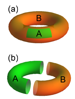
Figure 5: Two types of entanglement bipartitions on the torus: (a) A trivial bipartition with contractible boundaries for which the TEE $\gamma=\log D$, and (b) A bipartition with non-contractible boundaries, where the TEE depends on ground state.

V.2.1 Extracting Statistics from Topological Entanglement Entropy

As mentioned above, for Abelian phases, the $ij$’th entry of the $\mathcal{S}$ matrix corresponds to the phase the $i$’th quasi-particle acquires when it encircles the $j$’th quasi-particle. The $\mathcal{U}$ matrix is diagonal and the $ii$’th entry corresponds to the phase the $i$’th quasi-particle acquires when it is exchanged with an identical one. Since the MESs are the eigenstates of the nonlocal operators defined on the entanglement cut, the MESs are the canonical basis for defining $\mathcal{S}$ and $\mathcal{U}$. The modular matrices are just certain unitary transformations of the MES basis. For example,

$$\mathcal{S}_{\alpha\beta}=\frac{1}{D}\left\langle\Xi_{\alpha}^{\hat{x}}|\Xi_{\beta}^{\hat{y}}\right\rangle$$ (15)

Here $D$ is the total quantum dimension and $\hat{x}$ and $\hat{y}$ are two directions on a torus. Eqn.15 is just a unitary transformation between the particle states along different directions. In the case of a system with square geometry, the $\mathcal{S}$ matrix acts as a $\pi/2$ rotation on the MES basis $\left|\Xi_{\beta}^{\hat{y}}\right\rangle$. In general, however, $\hat{x}$ and $\hat{y}$ do not need to be geometrically orthogonal, and the system does not need to be rotationally symmetric, as long as the loops defining $\left|\Xi_{\alpha}^{\hat{x}}\right\rangle$ and $\left|\Xi_{\beta}^{\hat{y}}\right\rangle$ interwind with each other. We should mention one caveat with Eqn.15. When we write Eqn.15, we assume that the quasiparticles transform trivially under rotations. However, there exist topologically ordered states where rotations can induce a change in the quasiparticle type. For example, in the Wen-Plaquette model wenplaq , the rotations convert a charge-type excitation to a flux-type excitation. In such topological states, the procedure outlined above can give incorrect results, and we exclude such states from our discussion.

More concretely, let us denote the set of ground state wavefunctions as $|\xi_{\alpha}\rangle$ where $\alpha=1-N$ and $N$ is the total ground state degeneracy. To obtain the modular $S$ matrix, one calculates the minimum entropy states $|\Xi_{1,\alpha}\rangle$ and $|\Xi_{2,\alpha}\rangle$ for entanglement cuts along the directions $\vec{w}_{1}$ and $\vec{w}_{2}$ respectively. Doing so leads one to the matrices $U_{1}$ and $U_{2}$ that relates the states $|\xi_{\alpha}\rangle$ to $|\Xi_{1,\alpha}\rangle$ and $|\Xi_{2,\alpha}\rangle$ respectively. The modular $\mathcal{S}$ matrix is given by $U_{2}^{-1}U_{1}$ upto an undetermined phase for each MES. The existence of an identity particle that obtains trivial phase encircling any quasi-particle helps to fix the relative phase between different MESs, requiring the entries of the first row and column to be real and positive. This completely defines the modular $\mathcal{S}$ matrix. Therefore, the modular $\mathcal{S}$ matrix can be derived even without any presumed symmetry of the given wave functions.

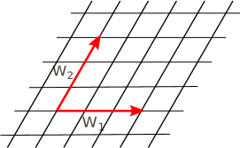
Figure 6: Vectors $\vec{w}_{1}$ and $\vec{w}_{2}$ that define a lattice with periodic boundary conditions. That is, any point $\vec{r}$ on the lattice satisfies $\vec{r}\equiv\vec{r}+\vec{w}_{1}\equiv\vec{r}+\vec{w}_{2}$. The area of the lattice is $|\vec{w}_{1}\times\vec{w}_{2}|$ where $\times$ denotes the cross product.

The above algorithm is able to extract the modular transformation matrix $\mathcal{S}$ and hence braiding and mutual statistics of quasi-particle excitations just using the ground-state wave functions as an input. Further, there is no loss of generality for non-Abelian phases, which can be dealt by enforcing the orthogonality condition in step $2$ which guarantees that one obtains states with quantum dimensions $d_{\alpha}$ in an increasing order. As shown in Ref. frank2012, , if the lattice has $2\pi/3$ rotation symmetry, then the operation of rotating MES states by an angle of $2\pi/3$ corresponds to the action of $\mathcal{US}$ on MES. Therfore, in the presence of such a symmetry, one can extract the $\mathcal{U}$ matrix as well.

V.2.2 Example: Semionic Statistics in Chiral Spin-Liquid from Entanglement Entropy

Let us revisit Chiral Spin-Liquid (CSL), first discussed in the Sec.V.1. Even though topological properties of CSL are well established using field-theoretic methods wen1990 , from a wavefunction point of view, CSL cannot be dealt with analytically unlike continuum Laughlin states. For example, the low energy theory of CSL predicts a particle with a semionic statistics (that is, the particle picks up a factor of -1 when it goes $2\pi$ around an identical one) which is difficult to verify in the lattice wavefunction directly. We will show that the entanglement based algorithm discussed in the last subsection readily demonstrates the existence of semion as an excitation in CSL.

As discussed in Sec.V.1, CSL corresponds to a d+id-wave state for chargeless spinons. The corresponding ground state wavefunction is obtained by Gutzwiller projecting the mean-field BCS ground state wavefunction. CSL has a topological ground-state degeneracy of two on torus. One of the ground states can be obtained by enforcing periodic boundary condition along $\hat{x}$-direction and anti-periodic along $\hat{y}$. We denote it by $|0,\pi\rangle$. The orthogonal ground state is given by $|\pi,0\rangle$ with the same notation.

Our task is to obtain the modular $\mathcal{S}$-matrix since it encodes the mutual statistics of quasiparticles. To do so, as outlined in the previous subsection, we consider linear combinations of $\left|0,\pi\right\rangle$ and $\left|\pi,0\right\rangle$:

$$\left|\Phi(\phi)\right\rangle=\cos\phi\left|0,\pi\right\rangle+\sin\phi\left|\pi,0\right\rangle$$ (16)

and numerically minimize the entanglement entropy with respect to the parameter $\phi$ so as to obtain the MESs frank2012 . For system with square geometry the $\mathcal{S}$ matrix describes the action of $\pi/2$ rotation on the MESs. Since the two states $|0,\pi\rangle$ and $|\pi,0\rangle$ transform into each other under $\pi/2$ rotation, this implies that $\mathcal{S}$ matrix is given by $V^{\dagger}\sigma_{x}V$ where $V$ is the unitary matrix that rotates the $\{|0,\pi\rangle\,|\pi,0\rangle\}$ basis to the MESs basis. From Fig.8, one finds that

$$V\approx\left(\begin{array}[]{cc}\cos(0.14\pi)&-\sin(0.14\pi)e^{i\varphi}\\ \sin(0.14\pi)&\cos(0.14\pi)e^{i\varphi}\end{array}\right)$$

The existence of an identity particle requires positive real entries in the first row and column and implies $\varphi=0$, which gives:

$$\mathcal{S}\approx\left(\begin{array}[]{cc}0.77&0.63\\ 0.63&-0.77\end{array}\right)=\frac{1}{\sqrt{2}}\left(\begin{array}[]{cc}1.08&0.89\\ 0.89&-1.08\end{array}\right)$$

which is in good agreement with the exact result

$$\mathcal{S}_{\textrm{exact}}=\frac{1}{\sqrt{2}}\left(\begin{array}[]{cc}1&1\\ 1&-1\end{array}\right)$$ (19)

Even though the $\mathcal{S}$ matrix obtained using our method is approximate, the quasiparticle statistics can be extracted exactly. In particular, the above $\mathcal{S}$ matrix tells us that the quasi-particle corresponding to $d_{0}=1$ does not acquire any phase when it goes around any other particle and corresponds to an identity particle as expected, while the quasi-particle corresponding to $d_{1/2}=1$ has semion statistics since it acquires a phase of $\pi$ when it encircles another identical particle. Numerical improvements can further reduce the error in pinpointing the MES and thereby leading to a more accurate value of the $\mathcal{S}$ matrix.

It is also interesting to compare the full dependence of TEE on the angle $\phi$. Theoretically, one finds the following expression for TEE dong2008 :

$$2\gamma-\gamma^{\prime} = \log\frac{4}{3+\sin\left(4\phi\right)}$$ (20)

where $\gamma$ is TEE for a region with contractible boundary while $\gamma^{\prime}$ is that for a region with non-contractible boundary. From Fig.8, we see that the numerically evaluated TEE is in rather good agreement with the exact expression.

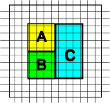
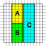
Figure 7: The separation of the system into subsystem $A$, $B$, $C$ and environment, periodic or antiperiodic boundary condition is employed in both $\hat{x}$ and $\hat{y}$ directions. a: The subsystem $ABC$ is an isolated square and the measured TEE has no ground state dependence. b: The subsystem $ABC$ takes a non-trivial cylindrical geometry and wraps around the $\hat{y}$ direction, and TEE may possess ground stated dependence.

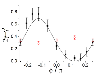
Figure 8: The black dots show the numerically measured TEE $2\gamma-\gamma^{\prime}$ for a CSL ground state from linear combination $\left|\Phi\right\rangle=\cos\phi\left|0,\pi\right\rangle+\sin\phi\left|\pi,0\right\rangle$ as a function of $\phi$ with VMC simulations frank2012 using geometry in Fig. 7b . Here $\gamma$ is TEE for a region with contractible boundary while $\gamma^{\prime}$ is that for a region with non-contractible boundary. The solid curve is the theoretical value from Eqn. 20. The periodicity is $\pi/2$. The red dots show the TEE for the same linear combination for a trivial bipartition. In the latter case, TEE is essentially independent of $\phi$ and again agrees rather well with the theoretical expectation (the dashed red curve).

VI Gapless QSLs and Entanglement

In this section we consider Gutzwiller projected Fermi liquid wave functions which are considered good ansatz for ground states of critical spin-liquids motrunich05 . We analyze two different classes of critical spin-liquids: states that at the slave-particle mean-field level have a full Fermi surface of spinons and those with only nodal spinons. The basic idea we use here is that for free fermions, the boundary law is violated by a multiplicative logarithm, that is, $S(l)\sim l^{d-1}\log(l)$ gioev2006 ; wolf . This suggests that for critical spin-liquids, whose low-energy theory contains a spinon Fermi surface mattergauge , a similar result might be expected. Indeed, one finds that for such Gutzwiller projected wavefunctions the entanglement entropy scales as $S(l)\sim l\log(l)$ for small system sizes frank2011crit . On the other hand, for wavefunctions with nodal spinons, the low-energy theory is believed to a two-dimensional CFT for which the result in Eqn.4 must hold. Thus, in this case, the VMC algorithm can be used to extract the universal shape dependent subleading constant.

The wave-functions for these spin-liquids are constructed by starting with a system of spin-$1/2$ fermionic spinons $f_{r\alpha}$ hopping on a finite lattice at half-filling with a mean field Hamiltonian:$H_{MF}=\sum_{rr^{\prime}}\left[-t_{rr^{\prime}}f^{\dagger}_{r\sigma}f_{r^{\prime}\sigma}+h.c.\right]$. The spin wave-function is given by $|\phi\rangle=P_{G}|\phi\rangle_{MF}$ where $|\phi\rangle_{MF}$ is the ground state of $H_{MF}$ and the Gutzwiller projector $P_{G}=\prod_{i}\left(1-n_{i\uparrow}n_{i\downarrow}\right)$ ensures exactly one fermion per site. The one dimensional case was discussed in Ref. Cirac, .

VI.1 Critical QSL with Spinon Fermi Surface

Consider the mean-field ansatz that describes spinons hopping on a triangular lattice. In this case, one might expect that the projected wavefunction describes the ground state of a QSL whose low energy theory contains a spinon Fermi surface motrunich05 ; mattergauge . Indeed, one finds frank2011crit that for a triangular lattice of total size $18\times 18$ on a torus and a subregion $A$ of square geometry with linear size $L_{A}$ up to 8 sites, the Renyi entropy scales as $L_{A}\,\textrm{log}L_{A}$ (Fig. 9). This is rather striking since the wave-function is a spin wave-function and therefore could also be written in terms of hard-core bosons. This result strongly suggests the presence of an underlying spinon Fermi surface. In fact the coefficient of the $L_{A}\,\textrm{log}L_{A}$ term is rather similar before and after projection. This observation may be rationalized as follows. Consider one dimensional fermions with $N$ flavors, where the central charge (and hence the coefficient of the $\log L_{A}$ entropy term) are proportional to $N$. However, Gutzwiller projection to single occupancy reduces the central charge to $N-1$. This is a negligible change for large $N$. Similarly, a two dimensional Fermi surface may be considered a collection of many independent one dimensional systems in momentum space, and Gutzwiller projection removes only one degree of freedom.

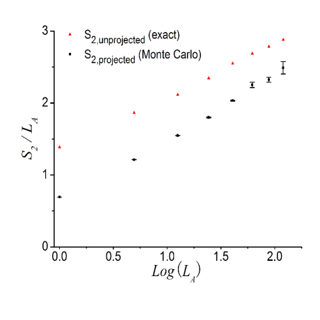
Figure 9: Renyi entropy data for the projected and unprojected Fermi sea state on the triangular lattice of size $18\times 18$ with $L_{A}=1-8$. Note, projection barely modifies the slope, pointing to a Fermi surface in the spin wavefunction.

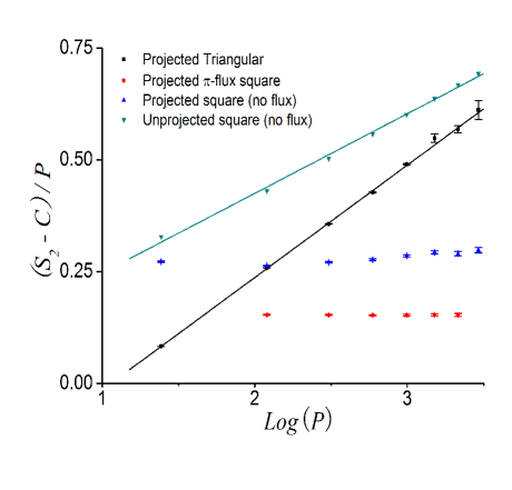
Figure 10: Comparison of the Renyi entropy data for the projected Fermi sea state on the triangular lattice and square (with and without $\pi$-flux) lattice as a function of the perimeter $P$ of the subsystem $A$. Here $C$ is the constant part of the $S_{2}$. We find $S_{2}\sim Plog(P)+C$ for the projected triangular lattice state while $S_{2}\sim P+C$ for the projected $\pi$-flux square lattice state. For the square lattice state (no flux), the projection leads to a significant reduction in $S_{2}$ and the data suggests at most a very weak violation of the area-law in the projected state.

The area-law violation of the Renyi entropy for Gutzwiller projected wave-functions substantiates the theoretical expectation that an underlying Fermi surface is present in the spin wavefunction.

VI.2 Critical QSL with Nodal Spinons

Next, consider a mean-field ansatz where the spinons hop on a square lattice with a flux $\pi$ through every plaquette piflux . Thus, at the mean-field level, one obtains spinons with Dirac dispersion around two nodes, say, $(\pi/2,\pi/2)$ and $(\pi/2,-\pi/2)$ (the location of the nodes depend on the gauge one uses to enforce the $\pi$ flux). The projected wave-function has been proposed in the past as the ground state of an algebraic spin liquid. The algebraic spin-liquid is believed to be describable by a strongly coupled conformal field theory of Dirac spinons coupled to a non-compact $SU(2)$ gauge field wen2002 ; wen2004 . Because of this the algebraic spin-liquid has algebraically decaying spin-spin correlations which can be verified explicitly using Variational Monte Carlo frank2011crit .

Square lattice being bipartite, the projected wavefunction satisfies Marshall’s sign rule and hence one is able to perform Monte Carlo calculation of Renyi entropy on bigger lattice sizes compared to the triangular lattice case. Consider an overall geometry of a torus of size $L_{A}\times 4L_{A}$, $L_{A}\leq 14$, with both region $A$ and its complement of sizes $L_{A}\times 2L_{A}$ (the total boundary size being $L_{A}+L_{A}=2L_{A}$). One finds frank2011crit that the projected wavefunction follows an area law akin to its unprojected counterpart and has the scaling $S_{2}\approx 0.31L_{A}+\gamma$ where $\gamma\approx 1.13$ is a universal constant that depends only on the aspect ratio of the geometry ryu2006 .

VI.3 Effect of Projection on Nested Fermi Surface

Finally, consider a mean-field ansatz as the fermions on a square lattice with nearest-neighbor hopping. The unprojected Fermi surface is nested. Since projection amounts to taking correlations into account, one might wonder whether the Fermi surface undergoes a magnetic instability after the projection. Indeed, one finds that the non-zero magnetic order in the projected wave-function frank2011crit , consistent with an independent study Ref. li2011, . This was verified by calculating spin-spin correlations on a $42\times 42$ lattice. Renyi entropy results for a a lattice of total size $24\times 24$ with region $A$ being a square up to size $12\times 12$ are shown in the Fig. 10. Though it is difficult to rule out presence of a partial Fermi surface from Renyi entropy, there is a significant reduction in the Renyi entropy as well as the coefficient of $L_{A}logL_{A}$ term as compared to the unprojected Fermi sea.

VII Synopsis and Recent Developments

In this article, we reviewed the perspective provided by the concept of entanglement entropy on QSLs. In particular, we discussed the practical uses of the concept of TEE to detect topological order in realistic QSLs and a detailed characterization of topological order using entanglement as well. Returning to the questions posed in the introduction, let us discuss whether entanglement entropy is of any value in finding new QSLs? Remarkably, one of the most accurate methods to study strongly correlated systems, namely, Density Matrix Renormalization Group (DMRG) white1992 , employs entanglement entropy as a resource to find ground states of particular Hamiltonians. In brief, DMRG implements a real-space renormalization group that successively coarse-grains the system on the basis of the entanglement between a sub-region and the rest of the system. Though DMRG is most accurate for one-dimensional quantum systems, recent works are now beginning to explore the realm of two-dimensional strongly correlated systems. As an output, DMRG yields an approximate ground state of the system along with the entanglement entropy for a bipartition of the system into two halves. Having access to the entanglement entropy implies that one can use the results reviewed in the previous sections, thus allowing one to establish (or rule out) a QSL ground state. As an example, using DMRG Yan et al yan2010 found that the ground state of kagome lattice Heisenberg Hamiltonian is a QSL. In a more recent study, Jiang et al hongchen2012 established the topological nature of this spin-liquid by calculating the TEE of the ground state for a region $A$ with non-contractible boundary and found it to be close to $\log(2)$, a value that is apparently consistent with that of a $Z_{2}$ QSL. Similar results are found for other models which are known to have topologically ordered ground states hongchen2012 . However, as discussed in Sec.V.2.1, TEE for a region with non-contractible boundary can be any number between 0 and $\log(2)$, the maximum value of TEE (hence minimum value for total entropy),being attained when the ground state corresponds to quasiparticle states. These results indicate that DMRG might be biased towards a linear combination of ground states that minimize total entropy. As discussed in Sec.V.2, entanglement can be used to determine quasiparticle statistics from a topologically degenerate set of ground states. Recently, using such an approach, Cincio and Vidal cincio extracted the modular $S$ and $U$ matrices for a microscopic lattice Hamiltonian that has a Chiral Spin Liquid ground state. Entanglement based measures have therefore emerged as a powerful conceptual and numerical tool in the context of quantum spin liquids. One may expect that in future, the confluence of ideas of many body physics and quantum information will throw up other equally fruitful directions.

Acknowledgements: We thank Ari Turner and Masaki Oshikawa for useful discussions and collaboration on the topics in this review. Support from NSF DMR- 0645691 and hospitality at KITP, Santa Barbara where part of this work was performed, is gratefully acknowledged. This research was supported in part by the National Science Foundation under Grant No. NSF PHY11-25915.

References

- (1) L. Balents, Nature 464, 199 (2010).
- (2) P. W. Anderson, Mater. Res. Bull. 8, 2 (1973).
- (3) P.W. Anderson, Science 237, 1196 (1987).
- (4) G. Baskaran, Z. Zou, P. Anderson, Solid State Comm. 63 973.
- (5) N. Read and S. Sachdev, Phys. Rev. Lett. 66, 1773 (1991); S. Sachdev, Physical Review B 45, 12377 (1992).
- (6) S. Kivelson, D. Rokhsar, J. Sethna, Phys. Rev. B 35, 8865-8868 (1987).
- (7) N. Read, B. Chakraborty, Phys. Rev. B 40, 7133 (1989).
- (8) T. Senthil, A. Vishwanath, L. Balents, S. Sachdev and M. P. A. Fisher, Science 303, 1490 (2004).
- (9) Y. Shimizu et al. Phys. Rev. Lett. 91, 107001 (2003), Y. Okamoto et al. Phys. Rev. Lett. 99. 137207 (2007), M. Yamashita et al, Science 328, 1246 (2010), J. S. Helton et al., Phys. Rev. Lett. 98, 107204 (2007).
- (10) Simeng Yan, David A. Huse, Steven R. White, Science 332, 1173 (2011).
- (11) Hong-Chen Jiang, Zhenghan Wang, Leon Balents, arXiv:1205.4289.
- (12) H.-C. Jiang, H. Yao, L. Balents, arXiv:1112.2241.
- (13) L. Wang, Z.-C. Gu, F. Verstraete, X.-G. Wen, arXiv:1112.3331.
- (14) Z. Y. Meng, T. C. Lang, S. Wessel, F. F. Assaad, A. Muramatsu, Nature 464, 847 (2010).
- (15) Xiao-Gang Wen, Quantum field theory of many-body systems, Oxford Graduate Texts, 2004.
- (16) M. B. Hastings, Phys. Rev. B 69, 104431 (2004).
- (17) see e.g. B. I. Halperin, P. A. Lee, and N. Read, Phys. Rev. B 47, 7312 (1993). B. L. Altshuler, L. B. Ioffe, and A. J. Millis, Phys. Rev. B 50, 14048 (1994). David F. Mross et al, Phys. Rev. B 82, 045121 (2010). Sung-Sik Lee, Phys. Rev. B 80, 165102 (2009).
- (18) A. Kitaev, J. Preskill, Phys. Rev. Lett. 96, 110404 (2010).
- (19) M. Levin, X.-G. Wen, Phys. Rev. Lett. 96, 110405 (2006).
- (20) T. Grover, A. Turner and A. Vishwanath, Phys. Rev. B 84, 075128 (2011).
- (21) B. Swingle, T. Senthil, arXiv:1109.3185v1.
- (22) Igor R. Klebanov, Silviu S. Pufu, Subir Sachdev, Benjamin R. Safdi, JHEP 1205, 036 (2012).
- (23) D. Gioev, I. Klich, Phys. Rev. Lett. 96, 100503 (2006).
- (24) M. M. Wolf, Phys. Rev. Lett. 96, 010404 (2006).
- (25) L. R. Bombelli. K. Koul, J. Lee, and R. D. Sorkin, Phys. Rev. D 34, 373 (1986).
- (26) M. Srednicki, Phys. Rev. Lett. 71, 66 (1993).
- (27) M. B. Hastings, J. Stat. Mech. , P08024 (2007).
- (28) J. Eisert, M. Cramer, M. B. Plenio, Rev. Mod. Phys. 82, 277 (2010).
- (29) S. Ryu, T. Takayanagi, JHEP 0608:045, 2006. H.Casini, M.Huerta, Nucl. Phys. B 764, 183 (2007).
- (30) P. Calabrese, J. Cardy, J. Stat. Mech. , P06002 (2004). C. Callan, F. Wilczek, Phys. Lett. B 333, 55 (1994). Holzhey, C., F. Larsen, and F. Wilczek, Nucl. Phys. B 424, 443 (1994).
- (31) A. Hamma, R. Ionicioiu, and P. Zanardi, Phys. Lett. A 337, 22 (2005); Phys. Rev. A 71, 022315 (2005).
- (32) A. Kitaev, Ann. Phys. 303, 2 (2003).
- (33) Michael A. Levin and Xiao-Gang Wen, Phys RevB. 71.045110 (2005).
- (34) Hui Li and F. D. M. Haldane , Phys. Rev. Lett. 101, 010504 (2008).
- (35) D. S. Rokhsar and S. A. Kivelson, Phys. Rev. Lett. 61, 2376 (1988).
- (36) R. Moessner, S. L. Sondhi, Phys. Rev. Lett. 86, 1881 (2001).
- (37) T. Senthil, O. Motrunich, Phys. Rev. B 66, 205104 (2002).
- (38) L. Balents, M.P.A. Fisher, S.M. Girvin, Phys. Rev. B 65, 224412 (2002).
- (39) G. Misguich, Phys.Rev.Lett. 89, 137202 (2002).
- (40) M. Gutzwiller, Phys. Rev. Lett. 10, 159 (1963);Phys. Rev. 134, A923 (1964);ibid. 137, A1726 (1965).
- (41) O. I. Motrunich, Phys. Rev. B 72, 045105 (2005).
- (42) Ying Ran, Michael Hermele, Patrick A. Lee, Xiao-Gang Wen, Phys. Rev. Lett. 98, 117205 (2007); Tocchio et al, Phys. Rev. B 80, 064419 (2010); T. Grover et al, Phys. Rev. B 81, 245121 (2010); B. K. Clark, D. A. Abanin, S. L. Sondhi, Phys. Rev. Lett. 107, 087204 (2011).
- (43) V. Kalmeyer and R. B. Laughlin, Phys. Rev. Lett. 59, 2095; V. Kalmeyer and R. B. Laughlin, Phys. Rev. B 39, 11 879; X. G. Wen, Frank Wilczek, and A. Zee, Phys. Rev. B 39, 11 413 (1989).
- (44) X.-G. Wen, Phys. Rev. B 44, 2664 (1991).
- (45) T. Senthil and M. P. A. Fisher. Phys. Rev. B 62, 7850 (2000).
- (46) E. Fradkin, S. Shenker, Phys. Rev. D 19, 3682-3697 (1979).
- (47) S. Papanikolaou, K. S. Raman, E. Fradkin, Phys. Rev. B 76, 224421 (2007).
- (48) F. D. M. Haldane, Phys. Rev. Lett. 60, 635 (1988). B. S. Shastry, Phys. Rev. Lett. 60, 639 (1988).
- (49) S.-S. Lee and P. A. Lee, Phys. Rev. Lett. 95, 036403 (2005).
- (50) M. Yamashita et al, Science 328, 1246 (2010). Y. Shimizu et al, Phys. Rev. Lett. 91, 107001 (2003). Y. Okamoto et al, Phys. Rev. Lett. 99, 137207 (2007).
- (51) M. B. Hastings et al., Phys. Rev. Lett. 104, 157201(2010).
- (52) C. Gros, Ann. Phys. 189, 53 (1989).
- (53) Yi Zhang, Tarun Grover, Ashvin Vishwanath, Phys. Rev. Lett. 107, 067202 (2011)
- (54) Yi Zhang, Tarun Grover, Ashvin Vishwanath, Phys. Rev. B 84, 075128 (2011).
- (55) S. Furukawa and G. Misguich, Phys. Rev. B 75, 214407 (2007).
- (56) Masudul Haque, Oleksandr Zozulya, and Kareljan Schoutens Phys. Rev. Lett. 98, 060401 (2007); O. S. Zozulya, M. Haque, K. Schoutens, and E. H. Rezayi, Phys. Rev. B 76, 125310 (2007).
- (57) A. Hamma, W. Zhang, S. Haas, and D. A. Lidar, Phys. Rev. B 77, 155111 (2008).
- (58) Sergei V. Isakov, Matthew B. Hastings, Roger G. Melko, arXiv:1102.1721.
- (59) D. F. Schroeter, E. Kapit, R. Thomale, and M. Greiter, Phys. Rev. Lett. 99, 097202 (2007).
- (60) Andreas W. W. Ludwig, Matthew P. A. Fisher, R. Shankar, G. Grinstein, Phys. Rev. B 50, 7526(1994).
- (61) E. Tang, J. W. Mei, and X. G. Wen, arXiv:1012.2930.
- (62) Yi-Fei Wang, Zheng-Cheng Gu, Chang-De Gong, D. N. Sheng, arXiv:1103.1686;D. N. Sheng, Zheng-Cheng Gu, Kai Sun, L. Sheng, arXiv:1102.2658v1.
- (63) T. Neupert, L. Santos, C. Chamon, and C. Mudry, arXiv:1012.4723.
- (64) K. Sun, Z. C. Gu, H. Katsura, and S. Das Sarma, arXiv:1012.5864.
- (65) X.-G. Wen, Int. J. Mod. Phys. B4, 239 (1990).
- (66) see e.g. Chetan Nayak, Steven H. Simon, Ady Stern, Michael Freedman, and Sankar Das Sarma, Rev. Mod. Phys. 80, 1083 (2008).
- (67) E. Keski-Vakkuri and Xiao-Gang Wen, Int. J. Mod. Phys. B7, 4227 (1993).
- (68) P. Di Francesco, P. Mathieu, D. Senechal, Conformal field theory, Springer 1997.
- (69) A. Kitaev Ann. Phys. 321, 2 (2006).
- (70) Erik P. Verlinde, Nucl. Phys. B300:360, (1988).
- (71) F.A. Bais, J.C. Romers, arXiv:1108.0683v1.
- (72) Shiying Dong, Eduardo Fradkin, Robert G. Leigh, Sean Nowling, JHEP 0805:016(2008).
- (73) Yi Zhang, Tarun Grover, Ari Turner, Masaki Oshikawa, Ashvin Vishwanath, Phys. Rev. B 85, 235151 (2012).
- (74) X.-G. Wen, Phys. Rev. Lett. 90, 016803 (2003).
- (75) We note that there are exceptions to the equality between the number of degenerate ground states and the number of quasiparticle types. For example, the Wen-Plaquette model wenplaq has a ground state degeneracy of two on an even odd torus, even though it is topologically ordered with four quasiparticle types.
- (76) J. I. Cirac, German Sierra, Phys. Rev. B 81, 104431 (2010).
- (77) I. Affleck and J. B. Marston, Phys. Rev. B 37, R3774 (1988), J. B. Marston and I. Affleck, Phys. Rev. B 39, 11538 (1989).
- (78) Xiao-Gang Wen, Phys. Rev. B 65, 165113 (2002).
- (79) Tao li, arXiv:1101.0193v1.
- (80) Steven R. White Phys. Rev. Lett. 69, 2863 (1992).
- (81) Lukasz Cincio, Guifre Vidal, arXiv:1208.2623v1.