Jet Mass Spectra in Higgs + One Jet at NNLL

Abstract

The invariant mass of a jet is a benchmark variable describing the structure of jets at the LHC. We calculate the jet mass spectrum for Higgs plus one jet at the LHC at next-to-next-to-leading logarithmic (NNLL) order using a factorization formula. At this order, the cross section becomes sensitive to perturbation theory at the soft $m_{\rm jet}^{2}/p_{T}^{\rm jet}$ scale. Our calculation is exclusive and uses the 1-jettiness global event shape to implement a veto on additional jets. The dominant dependence on the jet veto is removed by normalizing the spectrum, leaving residual dependence from non-global logarithms depending on the ratio of the jet mass and jet veto variables. For our exclusive jet cross section these non-global logarithms are parametrically smaller than in the inclusive case, allowing us to obtain a complete NNLL result. Results for the dependence of the jet mass spectrum on the kinematics, jet algorithm, and jet size $R$ are given. Using individual partonic channels we illustrate the difference between the jet mass spectra for quark and gluon jets. We also study the effect of hadronization and underlying event on the jet mass in Pythia. To highlight the similarity of inclusive and exclusive jet mass spectra, a comparison to LHC data is presented.

I Introduction

There has been a rapidly expanding theoretical and experimental effort on techniques that exploit the substructure of jets (for a recent review see Ref. Altheimer:2012mn ). Jet substructure is of interest both for testing QCD and for identifying new physics. Much of the excitement in this field has been driven by the excellent performance of the ATLAS and CMS detectors, and the sophisticated jet measurements this has made possible at the LHC. Jet substructure measurements can for example be used to tag boosted heavy particles, whose decay products get collimated into a fat jet, or to test and tune Monte Carlo programs. Most theoretical work has focused on designing these techniques and observables with the help of Monte Carlo programs. At the same time, one would also like to know that these methods are under theoretical control and build confidence that higher-order effects are not significant. (For some recent progress in this direction see e.g. Refs. Ellis:2009wj ; Bauer:2011uc ; Feige:2012vc ; Larkoski:2012eh ; Krohn:2012fg ; Waalewijn:2012sv .)

As our underlying hard process we consider $pp\to H+1$ jet with gluon fusion $gg\to H$ as the underlying Higgs production mechanism. This process is convenient as it provides a clean setup with a single quark or gluon jet in the final state via the three basic partonic channels $gg\to Hg$, $gq\to Hq$, and $q\bar{q}\to Hg$. Of course, it is also important in its own right for Higgs measurements at the LHC, which rely on exclusive jet channels.

Here we focus on one of the simplest jet substructures: the invariant mass of a jet. A successful calculation of this benchmark observable will instill confidence in our ability to carry out analogous calculations for other more complicated jet substructure observables. Such analyses require incorporating both a resummation of large logarithms $\alpha_{s}^{i}\ln^{j}(m_{J}^{2}/{p_{T}^{J\,2}})$ where $m_{J}$ is the jet mass and ${p_{T}^{J}}$ is the transverse momentum of the jet, as well as fixed-order perturbative corrections. This is made intricate by the dependence on multiple variables. There has been a lot of recent work on the calculation (resummation) of the jet invariant mass spectrum for jets with a realistic angular size Ellis:2009wj ; Ellis:2010rwa ; Jouttenus:2009ns ; Banfi:2010pa ; Kelley:2011tj ; Kelley:2011aa ; Li:2012bw ; Dasgupta:2012hg ; Chien:2012ur which we will review in more detail below. Some of the key theoretical issues that must be addressed for the LHC case include:

• Impact of summing large logarithms, $\ln(m_{J}^{2}/{p_{T}^{J\,2}})$

• Soft radiation effects at the scale $m_{J}^{2}/{p_{T}^{J}}$

• Impact of initial-state radiation

• Color flow and hard process dependence

• Dependence on kinematics including rapidity cuts

• Jet algorithm and dependence on jet size $R$

• Inclusive ($\geq N$ jets) vs. exclusive ($=N$ jets)

• Impact of non-global logarithms (NGLs)

• Effect of hadronization on the spectrum

• Effect of underlying event on the spectrum

• Effect of pile-up on the spectrum

• Utility of using groomed jets with trimming Krohn:2009th , filtering Butterworth:2008iy , or pruning Ellis:2009su

We now elaborate on several of these items. For a jet with ${p_{T}^{J}}\sim 300\,{\rm GeV}$, the jet mass peaks at $m_{J}\sim 50\,{\rm GeV}$, leading to large logarithms of ${p_{T}^{J\,2}}/m_{J}^{2}\sim 36$. Therefore, a description of the peak region of the jet mass spectrum requires the all-order resummation of these logarithms. Soft radiation with momentum $k^{\mu}\sim m_{J}^{2}/{p_{T}^{J}}$ is generated by both initial and final-state particles and contributes at leading order in the power expansion to the jet mass. Since fixed-order corrections start to become relevant for resummation at next-to-next-to-leading logarithmic (NNLL) order, a proper treatment of the soft scale $\sim m_{J}^{2}/{p_{T}^{J}}$ is crucial at this order Korchemsky:1999kt ; Bauer:2001yt ; Fleming:2007qr ; Ellis:2009wj . Numerically, the importance of these fixed-order soft corrections is also well known from recent work up to N³LL for event shapes in $e^{+}e^{-}\!\to$ jets Chien:2010kc ; Abbate:2010xh ; Chien:2012ur ; Gehrmann:2012sc . For processes with $\geq 2$ jets at hadron colliders there are multiple color structures, and the corresponding color flow must be taken into account starting at next-to-leading-logarithmic (NLL) order Dixon:2008gr .

The available freedom in defining a jet introduces a dependence of the jet mass spectrum on the choice of algorithm/clustering method and the jet size parameter $R$. There is also a choice of whether to use an inclusive or exclusive jet cross section, where the latter involves a veto on additional jets. The inclusive case has been studied at the LHC ATLAS:2012am , and inclusive calculations tend to focus on the anti-k_T algorithm Cacciari:2008gp . (Use of the anti-k_T jet algorithm avoids issues associated to clustering effects Banfi:2005gj ; Delenda:2006nf ; KhelifaKerfa:2011zu ; Kelley:2012kj .) As we will emphasize further below, a key difference between the inclusive and exclusive cases are the form of the non-global logarithms Dasgupta:2001sh ; Dasgupta:2002dc that arise at ${\cal O}(\alpha_{s}^{2})$ beyond the Born cross section due to multiple restrictions on phase space.

Let us summarize how the above issues have been studied so far in the literature on jet mass calculations. The first calculations were carried out for event shapes in $e^{+}e^{-}\!\to$ jets using hemisphere jet masses. Here factorization theorems are well established and calculations exist up to N³LL Clavelli:1979md ; Chandramohan:1980ry ; Clavelli:1981yh ; Korchemsky:1999kt ; Berger:2003iw ; Fleming:2007qr ; Fleming:2007xt ; Chien:2012ur . In Refs. Ellis:2009wj ; Ellis:2010rwa a factorization formula for exclusive $N$-jet cross sections at $e^{+}e^{-}$ colliders was derived, where the angularity of a jet (which includes the jet mass as a special case) is measured. This result only depends on the class of the jet algorithm (such as cone or k_T-type), but suffers from non-global logarithms involving the jet veto and jet size $R$. The resummation of the jet mass in $e^{+}e^{-}\!\to 2$ jets with a jet veto was carried out at NLL in Ref. Banfi:2010pa , which includes a resummation of NGLs in the large-$N_{c}$ approximation. This same process was considered in Ref. Kelley:2011tj , where the dominant $R$ dependence of asymmetric thrust (which is related to jet mass) was obtained using a refactorization of the soft function. In Ref. Kelley:2011aa , this refactorization was verified at ${\cal O}(\alpha_{s}^{2})$ and the leading NGLs were obtained at this order.

For jet mass calculations in $pp$ collisions one considers jets with large transverse momentum, $p_{T}^{J}$, and with rapidities $\eta^{J}$ away from the beam axis. Recently, several inclusive jet mass calculations have been carried out Li:2012bw ; Dasgupta:2012hg ; Chien:2012ur . In Ref. Li:2012bw , the jet mass was calculated using only a jet function. This ignores important contributions from wide-angle soft radiation, which couples together multiple hard partons, depends on the choice of jet algorithm, and contains NGLs. In Ref. Dasgupta:2012hg , the jet mass in $pp\to 2$ jets and $Z+1$ jet were calculated at NLL, including a resummation of NGLs in the large-$N_{c}$ approximation. Although this is an inclusive calculation (no jet veto), one should also note that hard emissions giving rise to additional jets are beyond the NLL order considered. In this case the dominant effect of the NGLs is on the peak of the jet mass distribution. Another inclusive calculation of the jet mass was carried out to obtain partial NNLL results in Ref. Chien:2012ur , by expanding around the threshold limit. Here dynamical threshold enhancement Appell:1988ie ; Catani:1998tm ; Becher:2007ty was used to argue that additional hard emissions are suppressed. Although NGLs were not resummed, their size was estimated, and found to mainly affect the peak region of the jet mass, as in Ref. Dasgupta:2012hg .

Our calculation at NNLL is for the exclusive jet mass spectrum, so it is useful to highlight differences with the inclusive case. At NLL, for a given partonic channel and fixed momenta of the hard partons, the two cases simply differ by a multiplicative factor, except for their respective NGLs. In both cases the lowest order NGLs involve terms of the form

$$\alpha_{s}^{2}\ln^{2}\Big{(}\frac{m_{J}^{\mathrm{cut}\,2}}{p_{\rm cut}^{2}}\Big{)}\,.$$ (1)

for the cumulant jet mass spectrum integrated up to $m_{J}^{\mathrm{cut}}$. For the inclusive jet mass spectrum, $p_{\rm cut}$ is a hard scale $\simeq p_{T}^{J}$ and the NGLs are therefore large logarithms that are parametrically of the same size as other $\alpha_{s}^{i}\ln^{j}(m_{J}^{2}/{p_{T}^{J\,2}})$ terms, and are thus part of the NLL result. Hence, in this case a complete resummation at NLL (or beyond) requires the NGLs to be resummed to all orders, which practically is currently only possible in the large-$N_{c}$ approximation. In contrast, in the exclusive case $p_{\rm cut}$ is an adjustable parameter and is related to the jet veto (in our analysis below we will have $p_{\mathrm{cut}}^{2}\simeq{p_{T}^{J}}\mathcal{T}^{\mathrm{cut}}$ where $\mathcal{T}^{\mathrm{cut}}$ implements the jet veto). In this case we have both $m_{J}^{2}\ll{p_{T}^{J\,2}}$ and $p_{\rm cut}^{2}\ll{p_{T}^{J\,2}}$, so the logarithms in Eq. (1) are smaller than in the inclusive case. In particular, for fixed $p_{\rm cut}$ there is a point in the $m_{J}$ spectrum where the NGLs vanish, and there is a region about this point where the NGLs are not large logarithms. An estimate for the size of this region can be obtained from the series of three NGL terms (log-squared, log, and non-log) that are known for the hemisphere jet masses Kelley:2011ng ; Hornig:2011iu . When all the terms in this series are of similar magnitude the logarithmic enhancement is not dominant, and the NGLs do not need to be resummed. This occurs for $1/8\leq m_{J}^{\mathrm{cut}\,2}/p_{\rm cut}^{2}\leq 8$. We will numerically explore the size of this region in our exclusive jet mass calculation, and demonstrate that the region is large enough that we may consider the non-global logarithms to not be large. This can be contrasted with Fig. 3 of Ref. Banfi:2010pa , which shows that the presence of an unmeasured region of phase space makes large NGLs unavoidable in the inclusive case Dasgupta:2012hg ; Chien:2012ur .

It should also be noted that although exclusive jet cross sections are not necessary for jet mass spectra, they are important in their own right because many Higgs and new physics searches categorize the data by the number of jets to improve their sensitivity. For example, the importance of the Higgs + 1 jet channel in $H\to\tau\tau$ and $H\to WW^{*}$ was pointed out in Refs. Mellado:2004tj ; Mellado:2007fb . Recently a NLL resummation of jet veto logarithms was carried out in the context of Higgs plus jets in Ref. Liu:2012sz .

Our calculation of the jet mass is centered on using the $N$-jettiness global event shape Stewart:2010tn to define jets, instead of a more traditional jet algorithm. For an event with $N$ jets, $N$-jettiness assigns all particles to $N+2$ regions, corresponding to the $N$ jets and two beams. We calculate the cross section for $pp\to H+1$ jet at NNLL, fully differential in the contributions of each region to $1$-jettiness. For the jet region, this contribution yields the jet invariant mass. The contribution from the remaining two beam regions are used to implement the jet veto. In each of these variables there is a series of large double logarithms that must be summed.

An advantage of using $N$-jettiness is that the jet veto is made through a jet mass-type variable, rather than a $p_{T}$ variable. Therefore, the structure of the perturbation theory, which is simultaneously differential in these two kinematic variables, is simpler. In particular, there is a QCD factorization formula for this cross section Stewart:2010tn ; Jouttenus:2011wh , obtained by making use of Soft-Collinear Effective Theory (SCET) Bauer:2000ew ; Bauer:2000yr ; Bauer:2001ct ; Bauer:2001yt . For the experimentally more realistic case of measuring $m_{J}$ with a $p_{T}$ veto variable one must simultaneously deal with a thrust-like invariant mass resummation and a $p_{T}$-type resummation.

Returning to our list of theoretical issues from the beginning, the use of $N$-jettiness allows us to carry out the summation of large logarithms at NNLL while properly accounting for soft radiation effects and initial-state radiation. We also use it to calculate the dependence of the jet mass spectrum on the jet kinematics, the jet size, and the definition of the jet region. Results are shown for individual partonic channels, $gg\to Hg$ and $gq\to Hq$, illustrating the differences between quark and gluon jets, as well as the full $pp\to H+1$ jet process from the Higgs coupling through a top quark loop. To investigate the differences between exclusive and inclusive jet mass measurements we compare our results with Pythia and also to ATLAS jet mass data ATLAS:2012am . We also analytically explore the effect of NGLs on the jet mass spectrum, and the effect of hadronization and underlying event with Pythia Sjostrand:2006za ; Sjostrand:2007gs .

Thus, we address all items in the bullet list of issues except for the last two, for which some brief comments are in order. Methods for removing pile-up contributions to jet observables have been discussed in e.g. Refs. Cacciari:2007fd ; Soyez:2012hv , and direct pile-up calculations are beyond the scope of our work. Finally, it is known that grooming jets has a large impact on their soft radiation and causes significant changes to the jet mass spectrum. We do not attempt to analytically control the effects of jet-grooming methods here.

In calculating the jet mass we consider both absolute and normalized spectra. Normalizing the jet mass spectrum reduces the perturbative uncertainty, and turns out to remove the dominant dependence on the jet veto variable. In particular, the jet veto dependence cancels up to NLL if we consider a particular partonic channel and fixed jet kinematics. We will show that this cancellation remains effective when summing over partonic channels and integrating over a range of kinematic variables.

In Sec. II, we discuss the kinematics and several jet definitions based on $N$-jettiness, exploring their features. The technical details of our calculation are presented in Sec. III. Here we discuss the factorization formula for the cross section, the refactorization of the soft function, non-global logarithms, and the choice of running scales. Sec. IV and Sec. V contain our numerical results for the individual partonic channels and for $pp\to H+1$ jet, showing the dependence of the jet mass spectrum on the jet veto cut, the order in perturbation theory, the jet kinematics, the jet definition, the jet area, on gluon versus quark jets, and on NGLs. Using Pythia8, in Sec. VI we analyze the hard process dependence for gluon jets, compare inclusive versus exclusive jet mass spectra, study the dependence on classic jet algorithms, and look at the impact of hadronization and underlying event. We also compare our NNLL exclusive jet results with Pythia for the same jet definition and kinematics, and compare them with inclusive jets from the LHC data. We conclude in Sec. VII. Detailed ingredients for the NNLL cross section are summarized in appendices.

II Kinematics and Jet Definitions

(a) Geometric $E$ and $p_{T}$ measures with $\rho=0.5$.

(b) Anti-k_T and geometric $R$ for $R=1$.

Figure 1: Comparison of the jet regions for different jet measures at different $\eta$ and $\phi$. The “$+$” marks the jet direction $\vec{n}_{J}$.

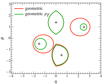
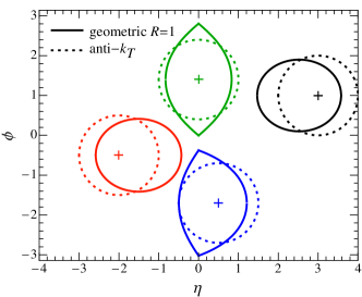
We describe the process $pp\to H+1$ jet using the transverse momentum $p_{T}^{J}$ of the jet, the pseudorapidity $\eta_{J}$ of the jet, and the rapidity $Y$ of the hard collision relative to the CM frame of the colliding protons. The $1$-jettiness event shape is defined as Stewart:2010tn

$$\mathcal{T}_{1}=\sum_{k}\min\Bigl{\{}\frac{2q_{J}\cdot p_{k}}{Q_{J}},\frac{2q_{a}\cdot p_{k}}{Q_{a}},\frac{2q_{b}\cdot p_{k}}{Q_{b}}\Bigr{\}}\,,$$ (2)

where $a,b$ denote the two beams and $J$ the jet, the $q_{i}$ are massless reference momenta and the $Q_{i}$ are normalization factors. For the reference momenta we take

$$q_{J}^{\mu}=E_{J}\,(1,\vec{n}_{J})\,,\qquad q_{a,b}^{\mu}=x_{a,b}\frac{E_{\mathrm{cm}}}{2}(1,\pm\hat{z})\,.$$ (3)

The jet energy $E_{J}$ and jet direction $\vec{n}_{J}$ can be predetermined with a suitable jet algorithm. The jet algorithm dependence this induces on $\mathcal{T}_{1}$ is power suppressed Stewart:2010tn , and we will use anti-k_T. The unit vector $\hat{z}$ points along the beam axis, and the momentum fractions $x_{a}$ and $x_{b}$ are fixed in terms of the total invariant mass $Q$ and rapidity $Y$,

$$x_{a}x_{b}E_{\mathrm{cm}}^{2} =Q^{2}=(q_{J}+q_{H})^{2}\,,$$

$$\ln\frac{x_{a}}{x_{b}} =2Y=\ln\frac{(1,-\hat{z})\cdot(q_{J}+q_{H})}{(1,\hat{z})\cdot(q_{J}+q_{H})}\,,$$ (4)

where $q_{H}^{\mu}$ denotes the momentum of the Higgs. For later convenience we also introduce the notation

$$s_{ij}=2q_{i}\cdot q_{j}\,.$$ (5)

The minimum in Eq. (2) divides the total phase space into $3$ regions, one for each beam and one for the jet. We denote their contributions to $\mathcal{T}_{1}$ as $\mathcal{T}_{a}$ and $\mathcal{T}_{b}$ for the two beam regions, and $\mathcal{T}_{J}$ for the jet region, so

$$\mathcal{T}_{1}=\mathcal{T}_{J}+\mathcal{T}_{a}+\mathcal{T}_{b}\,.$$ (6)

The contribution of the jet, $\mathcal{T}_{J}$, is directly related to the jet’s invariant mass $m_{J}$

$$m_{J}^{2} =p_{J}^{2}=(\bar{n}_{J}\cdot p_{J})(n_{J}\cdot p_{J})-\vec{p}_{J\perp}^{\>2}$$

$$=2q_{J}\cdot p_{J}\,[1+\mathcal{O}(\lambda^{2})]$$

$$=Q_{J}\mathcal{T}_{J}\,[1+\mathcal{O}(\lambda^{2})]\,,$$ (7)

where $p_{J}^{\mu}$ is the full jet momentum defined by summing all particles in the $\mathcal{T}_{J}$-region, $n_{J}^{\mu}=(1,\vec{n}_{J})$ and $\bar{n}_{J}^{\mu}=(1,-\vec{n}_{J})$ are defined by the predetermined jet direction $\vec{n}_{J}$, and the power counting parameter $\lambda$ scales as $\lambda^{2}\sim\mathcal{T}_{J}/E_{J}\sim m_{J}^{2}/E_{J}^{2}$. In the second line of Eq. (II) we used the fact that $\vec{n}_{J}$ and the exact direction of the $N$-jettiness jet, $\vec{p}_{J}$, differ by very little, such that $p_{J\perp}/(\bar{n}_{J}\cdot p_{J})\sim\lambda^{2}$. The difference between these two jet directions affects the jet boundary, which changes the contribution of soft radiation to the jet $p_{T}$, but only by a small amount $\sim\lambda^{2}$. We also used that the large jet momentum $\bar{n}_{J}\cdot p_{J}=\bar{n}_{J}\cdot q_{J}[1+\mathcal{O}(\lambda^{2})]$. For a jet with ${p_{T}^{J}}\sim 300\,{\rm GeV}$ these $\mathcal{O}(\lambda^{2})$ power corrections are $1/36\sim 3\%$ in the peak region, and hence negligible relative to the perturbative uncertainties at NNLL. Investigating the jet mass spectra for the exact $m_{J}^{2}=p_{J}^{2}$ vs. using $m_{J}^{2}=Q_{J}\mathcal{T}_{J}$ in Pythia, we also find that they are indistinguishable.

Figure 2: Numerical results for $\rho(R,\eta_{J})$ in the geometric $R$ measure. Left: Dependence on $R$ for $\eta_{J}=0$, which is $\sim R^{2}$ as expected. Right: Dependence on $\eta_{J}$ for $R=1$. To solve for $\rho$ we use a fit (solid line) to the true $\eta_{J}$ dependence (dots).

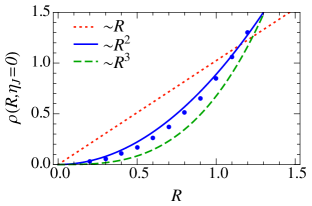
The details of the beam and jet regions selected by the minimum condition in Eq. (2) depend on the normalization factors $Q_{i}$. Since their values affect which particles are grouped into the beam and jet regions, they constitute a jet measure. They also impact the geometric shape of the jet area. Differences between measures are therefore similar to the different choices for jet-algorithms (anti-k_T, Cambridge-Aachen, cone, etc.). We will consider a variety of choices:

• invariant-mass measure:

  $$Q_{J}=Q_{a}=Q_{b}=Q$$ (8)

• geometric $p_{T}$ measure:

  $$Q_{J} =2\rho\,|\vec{q}_{iT}|=2\rho\,E_{J}/\cosh\eta_{J}$$ (9)

  $$Q_{a,b} =x_{a,b}E_{\mathrm{cm}}=e^{\pm Y}Q$$

• geometric measure:

  $$Q_{J} =2\rho\,E_{J}$$ (10)

  $$Q_{a,b} =x_{a,b}E_{\mathrm{cm}}=e^{\pm Y}Q$$

• geometric $R$ measure:

  $$Q_{J} =2\rho(R,\eta_{J})\,E_{J}$$ (11)

  $$Q_{a,b} =x_{a,b}E_{\mathrm{cm}}=e^{\pm Y}Q$$

  where $\rho(R,\eta_{J})$ fixes the area of the jet in $(\eta,\phi)$-space to be $\pi R^{2}$.

In all cases $\rho$ is a dimensionless parameter that allows one to change the size of the jet region. In the geometric $R$ case $\rho$ is fixed in terms of the jet radius parameter $R$. The choice of $Q_{a,b}$ in the geometric measures removes the dependence in $q_{a}^{\mu}/Q_{a}$ and $q_{b}^{\mu}/Q_{b}$ on the total rapidity $Y$. This is useful in the presence of missing energy, which prohibits the measurement of the boost $Y$ of the partonic center-of-mass frame. Note that the definitions of the measures through the $Q_{i}$ is influenced by the convention to use energies inside the $q_{i}^{\mu}$s in Eq. (3), since only the ratio $q_{i}^{\mu}/Q_{i}$ appears. Since for the geometric measures $Q_{J}\sim E_{J}$, they are all insensitive to the total jet energy. For the geometric $p_{T}$ case the jet is weighted by $E/p_{T}$ and we have explicitly

$$\frac{2q_{i}\cdot p_{k}}{{q}_{iT}} =p_{kT}\,\Bigl{(}2\frac{m_{kT}}{p_{kT}}\cosh\Delta y_{ik}\!-\!2\cos\Delta\phi_{ik}\Bigr{)}$$ (12)

where $\Delta y_{ik}=y_{i}-y_{k}$, $\Delta\phi_{ik}=\phi_{i}-\phi_{k}$ are the differences in rapidity and azimuthal angle between the direction of jet $i$ and particle $k$, and $m_{kT}^{2}=p_{kT}^{2}+m^{2}$ for a particle of mass $m$. For massless particles we thus get

$$\frac{2q_{i}\cdot p_{k}}{{q}_{iT}} =p_{kT}\,(2\cosh\Delta y_{ik}-2\cos\Delta\phi_{ik})$$

$$\approx p_{kT}\,\bigl{[}(\Delta y)^{2}+(\Delta\phi_{ik})^{2}\bigr{]}\,.$$ (13)

The jet regions for geometric $p_{T}$ and geometric are roughly circular, as shown in Fig. 1(a). They become smaller at large rapidities for geometric $p_{T}$, while they stay of comparable size for the geometric case.

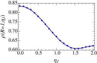
For geometric $R$, numerical results for the parameter $\rho(R,\eta_{J})$ as function of $R$ and $\eta_{J}$ are shown in Fig. 2. The left panel shows that the dependence on the jet radius $R$ is approximately $\rho\propto R^{2}$, as expected. The right panel illustrates the dependence on $\eta_{J}$ for fixed $R=1$, showing that $\rho$ approaches a constant for large $\eta_{J}$, i.e. when the jet becomes close to the beam. When using geometric $R$ in our results below, we use for convenience a fit of the $\eta_{J}$ dependence for fixed value of $R$. For example, for $R=0.5,0.7,1,1.2$ we have for $|\eta_{J}|\leq 2$

$$\rho(R=0.5,\eta_{J}) =0.164+0.037\eta_{J}^{2}-0.009\eta_{J}^{4}+0.0008\eta_{J}^{6}\,,$$

$$\rho(R=0.7,\eta_{J}) =0.357-0.040\eta_{J}^{2}+0.031\eta_{J}^{4}-0.005\eta_{J}^{6}\,,$$

$$\rho(R=1,\eta_{J}) =0.834-0.233\eta_{J}^{2}+0.077\eta_{J}^{4}-0.008\eta_{J}^{6}\,,$$

$$\rho(R=1.2,\eta_{J}) =1.272-0.377\eta_{J}^{2}+0.101\eta_{J}^{4}-0.010\eta_{J}^{6}\,.$$ (14)

Note that for $R=0.5$ the parameter $\rho$ increases rather than decreases with $\eta_{J}$. A comparison of the jet regions for geometric $R$ with anti-k_T jets is shown in Fig. 1(b). Although their areas are chosen to be the same, the geometric $R$ jets are not perfectly circular and have an “offset” between the jet direction and the center of the jet region. The former (latter) effect decreases (increases) with $|\eta_{J}|$. For a smaller jet radius of $R=0.5$ the geometric $R$ jets become more circular also at central rapidities and are very close to anti-k_T jets. In Ref. Thaler:2011gf a modification of $N$-jettiness was introduced that matches anti-k_T closely for any $R$. However, this definition reintroduces a region of phase space that belongs neither to the jet nor the beams, making it more complicated for calculations.

III Calculation

channel	$\kappa_{a}$	$\kappa_{b}$	$\kappa_{J}$
$gg\to Hg$	$g$	$g$	$g$
$gq\to Hq$	$g$	$q$	$q$
$qg\to Hq$	$q$	$g$	$q$
$g\bar{q}\to\bar{H}q$	$g$	$\bar{q}$	$\bar{q}$
$\bar{q}g\to\bar{H}q$	$\bar{q}$	$g$	$\bar{q}$
$q\bar{q}\to Hg$	$q$	$\bar{q}$	$g$
$\bar{q}q\to Hg$	$\bar{q}$	$q$	$g$

Table 1: Values of $\kappa$ for the different partonic channels.

III.1 Factorization Formula

We start by rewriting the phase space integrals for the hard kinematics in terms of the rapidity $\eta_{J}$ and transverse momentum $p_{T}^{J}$ of the jet and the total rapidity $Y$,

$$\int\!\frac{\mathrm{d}x_{a}}{x_{a}}\!\int\!\frac{\mathrm{d}x_{b}}{x_{b}}\!\int\frac{\mathrm{d}^{3}\vec{q}_{H}}{(2\pi)^{3}}\frac{1}{2E_{H}}\!\int\!\frac{\mathrm{d}^{3}\vec{q}_{J}}{(2\pi)^{3}}\frac{1}{2E_{J}}\,$$

$$\quad\times(2\pi)^{4}\delta^{4}\bigl{(}q_{a}+q_{b}-q_{J}-q_{H}\bigr{)}$$

$$\qquad=\int\!\mathrm{d}\eta_{J}\,\mathrm{d}p_{T}^{J}\,\mathrm{d}Y\,\frac{1}{2\pi}\frac{p_{T}^{J}}{Q^{2}+m_{H}^{2}}\,.$$ (15)

The variables were defined in Sec. II, and we used azimuthal symmetry and the relations

$$p_{T}^{J} =\frac{Q^{2}-m_{H}^{2}}{2Q\cosh(\eta_{J}-Y)}\,,$$ (16)

$$Q =p_{T}^{J}\cosh(\eta_{J}-Y)+\sqrt{p_{T}^{J\,2}\cosh^{2}(\eta_{J}-Y)+m_{H}^{2}}\,.$$

Many of our plots will be normalized and for fixed values of $\eta_{J}$, $p_{T}^{J}$, and $Y$, in which case the phase space factor in Eq. (III.1) drops out.

Our calculation relies on the $N$-jettiness factorization formula in Ref. Jouttenus:2011wh , which we here specialize to the case of $1$-jettiness:

$$\frac{\mathrm{d}^{3}\sigma^{H+1j}}{\mathrm{d}\eta_{J}\,\mathrm{d}p_{T}^{J}\,\mathrm{d}Y\,\mathrm{d}\mathcal{T}_{a}\,\mathrm{d}\mathcal{T}_{b}\,\mathrm{d}\mathcal{T}_{J}} =\frac{p_{T}^{J}}{4\pi E_{\mathrm{cm}}^{2}(Q^{2}+m_{H}^{2})}\sum_{\kappa}H_{\kappa}(\{q_{i}^{\mu}\},\mu)\int\!\mathrm{d}t_{a}\,B_{\kappa_{a}}(t_{a},x_{a},\mu)\int\!\mathrm{d}t_{b}\,B_{\kappa_{b}}(t_{b},x_{b},\mu)$$

$$\quad\times\int\!\mathrm{d}s_{J}\,J_{\kappa_{J}}(s_{J},\mu)\,S_{\kappa}\biggl{(}\mathcal{T}_{a}-\frac{t_{a}}{Q_{a}},\mathcal{T}_{b}-\frac{t_{b}}{Q_{b}},\mathcal{T}_{J}-\frac{s_{J}}{Q_{J}},\Big{\{}\frac{q_{i}^{\mu}}{Q_{i}}\Big{\}},\mu\biggr{)}\,\,.$$ (17)

The $N$-jettiness variables $\mathcal{T}_{a}$, $\mathcal{T}_{b}$, and $\mathcal{T}_{J}$ were defined in Sec. II. The hard function $H_{\kappa}$ contains the short-distance matrix element for producing a Higgs plus a jet, the beam functions $B_{\kappa_{a}}$ and $B_{\kappa_{b}}$ describe the collinear initial-state radiation and contain the PDFs, the jet function $J_{\kappa_{J}}$ characterizes the collinear final-state radiation, and the soft function $S_{\kappa}$ describes soft radiation effects. The sum over $\kappa=\{\kappa_{a},\kappa_{b},\kappa_{J}\}$ runs over the possible flavors $\kappa_{i}\in\{g,u,\bar{u},d,\dots\}$ of the two incoming and one outgoing parton. The possible combinations, corresponding to the various partonic channels, are listed in Table 1.

The power of factorization is that it allows one to evaluate the various fixed-order pieces at their natural scales, where they contain no large logarithms. We then use the RG evolution of each of these functions to evolve them to a common scale $\mu$, resumming the logarithms of $m_{J}^{2}/{p_{T}^{J\,2}}$ and $Q_{i}\mathcal{T}_{i}/{p_{T}^{J\,2}}$. This evolution is implicit in Eq. (III.1), by writing all functions as evaluated at the common scale $\mu$. The factorization formula with all evolution factors written out explicitly is given in Eq. (III.2) below. Our choice of scales is discussed in Sec. III.3. Power corrections to Eq. (III.1) arise from so-called nonsingular corrections, which are suppressed by a relative $\mathcal{O}(m_{J}^{2}/Q^{2})$ in this differential cross section, and are not considered here.

The cross section in Eq. (III.1) is differential in the $1$-jettiness contributions from the jet and the beams $\mathcal{T}_{J}$, $\mathcal{T}_{a}$, and $\mathcal{T}_{b}$. As we will see, the shape of the jet mass spectrum is independent of the jet veto for a reasonable range of $\mathcal{T}_{a,b}$ values. For simplicity we impose a common cut $\mathcal{T}_{a,b}\leq\mathcal{T}^{\mathrm{cut}}$. We also convert $\mathcal{T}_{J}$ to the jet mass $m_{J}$ using Eq. (II), and so consider

$$\sigma(m_{J}^{\mathrm{cut}},\mathcal{T}^{\mathrm{cut}}) =\int_{0}^{\mathcal{T}^{\mathrm{cut}}}\!\!\!\!\!\!\!\!\!\!\mathrm{d}\mathcal{T}_{a}\!\int_{0}^{\mathcal{T}^{\mathrm{cut}}}\!\!\!\!\!\!\!\!\!\!\mathrm{d}\mathcal{T}_{b}\!\int_{0}^{m_{J}^{\mathrm{cut}\,2}/Q_{J}}\!\!\!\!\!\!\!\!\!\!\!\!\!\!\mathrm{d}\mathcal{T}_{J}\>\,\frac{\mathrm{d}^{3}\sigma}{\mathrm{d}\mathcal{T}_{a}\,\mathrm{d}\mathcal{T}_{b}\,\mathrm{d}\mathcal{T}_{J}}\,.$$ (18)

The differential jet mass cross section, $\mathrm{d}\sigma/\mathrm{d}m_{J}$, is obtained by taking the numerical derivative of this cumulant cross section. We define the normalized jet mass spectrum over the range $[0,m_{J}^{\mathrm{cut}}]$ as $\mathrm{d}\hat{\sigma}/\mathrm{d}m_{J}$, so

$$\frac{\mathrm{d}\hat{\sigma}}{\mathrm{d}m_{J}}(m_{J}^{\mathrm{cut}},\mathcal{T}^{\mathrm{cut}})\equiv\frac{1}{\sigma(m_{J}^{\mathrm{cut}},\mathcal{T}^{\mathrm{cut}})}\frac{\mathrm{d}\sigma(\mathcal{T}^{\mathrm{cut}})}{\mathrm{d}m_{J}}\,.$$ (19)

The ingredients in the resummed cross section are needed at different orders in perturbation theory, as summarized in Table 2, where the columns correspond to the fixed-order matching, non-cusp anomalous dimension $\gamma_{x}$, cusp anomalous dimension $\Gamma_{\mathrm{cusp}}$, the $\beta$ function, and the PDFs. All ingredients necessary for a NNLL resummation of the global logarithms are known and are collected in App. A: The one-loop hard function for the three basic processes $gg\to Hg$, $gq\to Hq$, and $q\bar{q}\to Hg$ via gluon fusion (in the large $m_{t}$ limit) are obtained from the one-loop helicity amplitudes calculated in Ref. Schmidt:1997wr following the procedure in Ref. Stewart:2012yh . The one-loop quark and gluon jet function were calculated in Refs. Bauer:2003pi ; Fleming:2003gt ; Becher:2009th , the one-loop quark and gluon beam functions in Refs. Stewart:2009yx ; Stewart:2010qs ; Mantry:2009qz ; Berger:2010xi , and the one-loop soft function in Ref. Jouttenus:2011wh . We also require the cusp anomalous dimension to three loops Korchemsky:1987wg ; Moch:2004pa , and the non-cusp anomalous dimensions to two loops, which are known from Refs. Kramer:1986sg ; Harlander:2000mg ; MertAybat:2006mz ; Becher:2006qw ; Becher:2009th ; Stewart:2010qs .

	matching	$\gamma_{x}$	$\Gamma_{\mathrm{cusp}}$	$\beta$	PDF
LL	$0$-loop	-	$1$-loop	$1$-loop	NLO
NLL	$0$-loop	$1$-loop	$2$-loop	$2$-loop	NLO
NNLL	$1$-loop	$2$-loop	$3$-loop	$3$-loop	NLO

Table 2: Perturbative ingredients at different orders in resummed perturbation theory.

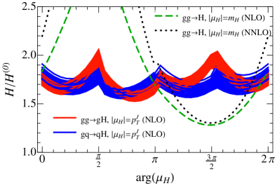
There is some freedom in how to treat products of the fixed-order corrections in Eq. (III.1), specifically the higher-order cross terms that are generated, such as the one-loop correction to $H$ times the one-loop correction to $J$, which we denote $H^{(1)}J^{(1)}$. The series for the individual objects are fairly convergent, except for the hard function whose one-loop correction is known to be rather large. For the hard function in $pp\to H+0$ jets the use of a complex scale, $\mu_{H}=-{\mathrm{i}}\,m_{H}$ improves the perturbative convergence Ahrens:2008qu , since this $H$ is related to the time-like scalar form factor. For $pp\to H+1$ jet the hard functions contain logarithms with both positive and negative arguments, so some logarithms are minimized by an imaginary $\mu_{H}$ and others by a real $\mu_{H}$. The convergence for the hard functions for both $pp\to H+0$ jets and $pp\to H+1$ jet are shown in Fig. 3 as a function of the complex phase chosen for $\mu_{H}$. For $pp\to H+0$ jets the improvement in the convergence for $\arg(\mu_{H})=3\pi/2$ is clearly visible, while for $pp\to H+1$ jets the convergence is only marginally affected by the choice of $\arg(\mu_{H})$. Therefore we alway use $\arg(\mu_{H})=0$ for our analysis here.

Figure 3: Hard functions for $gg\to H$ at NLO and NNLO, and for $gg\to Hg$ and $gq\to Hq$ at NLO as a function of the phase used in their scale $\mu_{H}$. For the $gg\to Hg$ and $gq\to Hq$ the results are bands because we scan over kinematics in the range $200<{p_{T}^{J}}<600\,{\rm GeV}$, $0<\eta_{J}<1$, and $0<Y<1$.

When combining the perturbative series from different functions in the factorization theorem, we always expand the convolutions of the fixed-order $B$, $J$, and $S$ functions order by order in $\alpha_{s}$ to the order needed, but consider two possibilities for the hard function $H^{(0)}+H^{(1)}$, either expanded along with the other functions or kept as an overall multiplicative factor. The difference between expanding the hard function or treating it as multiplicative is within our perturbative uncertainty, being a $\lesssim 20\%$ effect for the unnormalized $m_{J}$ spectrum, and only a $\lesssim 2\%$ effect for the normalized $m_{J}$ spectrum. When $H$ is expanded out there is also $\sim 2\%$ increase in the perturbative uncertainties for the normalized $m_{J}$ spectrum for $gg\to Hg$, so we pick this convention as our default in order to be conservative. Schematically, this means that the fixed-order components of our cross section take the form

$$H^{(0)}\Bigl{[}(B^{(0)}B^{(0)}J^{(0)})\otimes S^{(0)}$$ (20)

$$\quad+(B^{(1)}B^{(0)}J^{(0)})\otimes S^{(0)}+(B^{(0)}B^{(1)}J^{(0)})\otimes S^{(0)}$$

$$\quad+(B^{(0)}B^{(0)}J^{(1)})\otimes S^{(0)}+(B^{(0)}B^{(0)}J^{(0)})\otimes S^{(1)}\Bigr{]}$$

$$\quad+H^{(1)}(B^{(0)}B^{(0)}J^{(0)})\otimes S^{(0)}\,.$$

III.2 Refactorization of the Soft Function

For a process with one or more jets there are multiple directions for collinear radiation and various kinematic variables so a few additional hierarchies become possible. The factorization formula assumes that there are no additional strong hierarchies beyond the collinearity of the jet $m_{J}^{2}\ll{p_{T}^{J\,2}}$, and the absence of additional central jets away from the beam directions, $Q_{a}\mathcal{T}_{a}\ll{p_{T}^{J\,2}}$ and $Q_{b}\mathcal{T}_{b}\ll{p_{T}^{J\,2}}$. Physically, the absence of no additional strong hierarchies corresponds to the following four assumptions

1. $Q_{i}\mathcal{T}_{i}\sim Q_{j}\mathcal{T}_{j}$  commensurate $m_{J}$ and jet veto

2. $\dfrac{q_{i}\cdot q_{j}}{E_{i}E_{j}}\sim\dfrac{q_{i}\cdot q_{k}}{E_{i}E_{k}}$  well separated jet and beams

3. $E_{i}\sim E_{j}$   jet and beam-jets of similar energy

4. $Q_{i}\sim Q_{j}$   jet and beam regions of similar size

Assumption 1) ensures that we are in the region where NGLs are not large logarithms. Assumption 2) implies that the jet is not too close to the beam direction, and avoids having large angular logarithms, which would require an additional “ninja summation” Bauer:2011uc .

Three combinations of these four assumptions are necessary to avoid introducing additional large logarithms that are not summed by the renormalization group evolution of terms in the factorization formula, namely

$$\frac{s_{ij}}{s_{ik}}\sim 1\,, \frac{\mathcal{T}_{i}}{\mathcal{T}_{j}} \sim 1\,, \frac{Q_{i}}{Q_{j}} \sim 1\,.$$ (21)

The first implies that the logarithms in the hard function can be minimized with a common scale $\mu$, and all three combine to imply that a common scale also minimizes all logarithms in the soft function. One combination of assumptions, $E_{i}/Q_{i}\sim E_{j}/Q_{j}$, does not appear explicitly in arguments of functions in the factorized cross section, and hence does not show up in logarithms for the leading power result. However, it is in general necessary as part of the derivation of Eq. (III.1) to ensure that certain neglected terms are power suppressed.

An important consideration in carrying out the summation of large logarithms is the order in $\alpha_{s}$ and logarithms at which violations of Eq. (21) first become apparent. For the soft function the first terms that appear for the various logarithms are

$$\alpha_{s}\ln^{2}\Bigl{(}\frac{Q_{i}\mathcal{T}_{i}^{c}Q_{j}\mathcal{T}_{j}^{c}}{\mu^{2}s_{ij}}\Bigr{)}\,, \alpha_{s}\ln\Bigl{(}\frac{s_{ij}Q_{k}}{s_{ik}Q_{j}}\Bigr{)} \,, \alpha_{s}^{2}\ln^{2}\Bigl{(}\frac{\mathcal{T}_{i}^{c}}{\mathcal{T}_{j}^{c}}\Bigr{)}\,,$$ (22)

where we integrate the soft function over $\mathcal{T}_{i}$ up to the cumulant variable $\mathcal{T}_{i}^{c}$. The first of these is part of the LL series. The second is an angular logarithm. It is part of the NLL series if it counts as a large logarithm. Otherwise, it is part of the $\sim\alpha_{s}$ fixed-order terms that start to contribute at NNLL. The third is a NGL. It is part of the NLL series if it is a large logarithm. Otherwise it is part of the $\sim\alpha_{s}^{2}$ fixed-order terms that start to contribute at N³LL. Therefore, there is a nontrivial constraint on the choice of scales $\mu$ in the soft function. The scales must be chosen to minimize the first type of logarithm in Eq. (22) without inducing terms of the form of the second and third types already at LL order. In particular, this implies that a poor scale choice could introduce unphysical angular logarithms or NGLs into the LL series. For our choice of kinematics and $Q_{i}$ the second type of angular logarithm in Eq. (22) is never large. However, since we are exploring a spectrum in $m_{J}^{2}=Q_{J}\mathcal{T}_{J}$ the third term in Eq. (22) will grow as the parameters are varied. To surmount this problem requires a refactorization of the soft function which we will consider below.

For the hard function the series of leading double logarithms involves terms of the form

$$\alpha_{s}\ln^{2}\Bigl{(}\frac{\mu^{2}}{s_{ij}}\Bigr{)}\,, \alpha_{s}\ln^{2}\Bigl{(}\frac{s_{ij}}{s_{ik}}\Bigr{)}\,.$$ (23)

For the choice of jet kinematics explored in this paper we will always satisfy the assumption $s_{ij}\sim s_{ik}$, so there is no additional constraint on the scale associated with the hard function.

The hierarchy between $\mathcal{T}_{J}$ and $\mathcal{T}^{\mathrm{cut}}$ leads to unphysical large logarithms if a single scale $\mu_{S}$ is used for the initial conditions for the soft function evolution. Here we address how these can be removed by a refactorization of the soft function, with corrections from the true higher order non-global logarithms (see Refs. Fleming:2007xt ; Ellis:2010rwa ; Kelley:2011aa ; Chien:2012ur for earlier refactorization discussions).

In general, the all-order soft function has the form

$$S(\{k_{i}\},\{\hat{q}_{i}^{\mu}\},\mu)$$

$$\quad=\prod_{i}S_{i}(k_{i},\{\hat{q}_{i}^{\mu}\},\mu)+S_{\rm NGL}(\{k_{i}\},\{\hat{q}_{i}^{\mu}\},\mu)\,,$$ (24)

where $\hat{q}_{i}^{\mu}=q_{i}^{\mu}/Q_{i}$. Here $S_{\rm NGL}$ contains all non-global terms, and hence has an intrinsic dependence on the ratios $k_{i}/k_{j}$. At NLO there is only one soft gluon emitted, which can contribute to only one of the $\mathcal{T}_{i}$ at a time. Thus the NLO soft function factorizes, and $S_{\rm NGL}\sim\mathcal{O}(\alpha_{s}^{2})$. Truncating to $\mathcal{O}(\alpha_{s})$ there is still some freedom in the definition of the $S_{i}$. Whereas the terms with explicit $k_{i}$ dependence in $S(\{k_{i}\},\mu)$ clearly belong to $S_{i}(k_{i},\mu)$, the pure delta function terms $\delta(k_{J})\delta(k_{a})\delta(k_{b})$ can in principle be split in multiple ways between the various $S_{i}(k_{i},\mu)$. We choose to split these terms evenly, as detailed in App. A.4, and we introduce an additional parameter $r$ in the scale variation to estimate uncertainty from this freedom as discussed further below and in detail in Sec. III.3.

Due to the consistency of the factorization formula, the evolution of the soft function factorizes exactly to all orders in perturbation theory,

$$U_{S}(\{k_{i}\},\mu,\mu_{0}) =U_{H}(\mu_{0},\mu)\prod_{i}Q_{i}U_{J_{i}}(Q_{i}k_{i},\mu_{0},\mu)$$

$$=\prod_{i}U_{S_{i}}(k_{i},\mu,\mu_{0})\,.$$ (25)

Note that this result does not rely on the refactorization of the soft function discussed above. (Here we used the fact that the beam and jet functions have the same evolution Stewart:2010qs .) Equation (III.2) involves the factorization of the evolution of the hard function $H=CC^{\dagger}$, which follows from the form of the anomalous dimension for $C$ Chiu:2008vv ; Becher:2009qa ,

$$\widehat{\gamma}_{C}(\mu) =-\Gamma_{\mathrm{cusp}}[\alpha_{s}(\mu)]\bigg{[}\sum_{i}\mathbf{T}_{i}^{2}\ln\frac{\mu}{\mu_{0}}$$

$$\quad+\sum_{i<j}\mathbf{T}_{i}\!\cdot\!\mathbf{T}_{j}\,\ln\Bigl{(}-\frac{s_{ij}}{\mu_{0}^{2}}\!-\!\mathrm{i}0\Bigr{)}\bigg{]}+\widehat{\gamma}_{C}[\alpha_{s}(\mu)]\,.$$ (26)

The sum on $i$ and $j$ runs over the colored partons participating in the short-distance interaction and $\mathbf{T}_{i}$ denotes the corresponding color charge matrix. (For $pp\to H+1$ jet the color space is still trivial, so these color matrices are just numbers.) To associate the $\ln\mu$ terms to individual partons we introduced a dummy variable $\mu_{0}$ and used color conservation. It is not a priori clear how to associate the remaining terms within the $\sum_{i<j}$ to each $U_{S_{i}}$, and we choose to split each term evenly between $i$ and $j$. The explicit expression for the factorized hard function evolution that we employ is given in App. A.5. Other potential choices of splitting up these terms are again probed by the scale parameter $r$, which is discussed in more detail around Eq. (III.3), and the corresponding uncertainty is found to be small except on the large $m_{J}$ tail of the distribution. The two-loop non-cusp anomalous dimension has the structure $\widehat{\gamma}_{C}(\alpha_{s})=n_{q}\gamma_{q}+n_{g}\gamma_{g}$, where $n_{g}$ and $n_{q}$ are the number of gluon and (anti)quark legs, so it naturally factors.

Figure 4: Illustration of the different fixed-order scales appearing in the factorized cross section and our evolution strategy. The figure has $Y=0$ where there is a common $\mu_{B}$ scale.

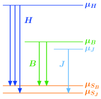
The factorization of the evolution and fixed-order soft function in Eqs. (III.2) and (III.2) suggests that we can evaluate the piece of the soft function corresponding to $\mathcal{T}_{i}$ at a scale $\mu_{S_{i}}$,

$$S(\{k_{i}\},\mu)=\prod_{i}\!\int\!\mathrm{d}k_{i}^{\prime}\,U_{S_{i}}(k_{i}-k_{i}^{\prime},\mu,\mu_{S_{i}})S_{i}(\{k_{i}^{\prime}\},\mu_{S_{i}})\,.$$ (27)

This factorization does not hold for all the terms at order $\alpha_{s}^{2}$, since there are diagrams that contribute to multiple $\mathcal{T}_{i}$, leading to non-global logarithms of the form $\alpha_{s}^{2}\ln^{2}(k_{i}^{c}/k_{j}^{c})$ appearing in $S_{\rm NGL}$ in Eq. (III.2). We discuss in Sec. III.4 how we estimate the size of these NGL contributions in the jet mass spectrum.

In our implementation we find it simplest to run the hard, jet, and beam functions, rather than the soft function, as summarized in Fig. 4. The final results are completely independent of this choice. Since the cut on both beams is the same, they have a common $\mu_{S_{B}}$, and a common $\mu_{B}$ for $Y=0$. We summarize the work in this section by presenting the factorization formula valid at NNLL which includes the evolution factors and refactorization of $S$,

$$\frac{\mathrm{d}^{3}\sigma^{H+1j}(\mathcal{T}^{\mathrm{cut}})}{\mathrm{d}\eta_{J}\,\mathrm{d}p_{T}^{J}\,\mathrm{d}Y\,\mathrm{d}m_{J}} =\frac{(2p_{T}^{J}m_{J}/Q_{J})}{4\pi E_{\mathrm{cm}}^{2}(Q^{2}+m_{H}^{2})}\sum_{\kappa}H_{\kappa}(\{q_{i}^{\mu}\},\mu_{H})U_{H_{\kappa_{a}}}(\{q_{i}^{\mu}\},\mu_{S_{B}},\mu_{H})U_{H_{\kappa_{b}}}(\{q_{i}^{\mu}\},\mu_{S_{B}},\mu_{H})U_{H_{\kappa_{J}}}(\{q_{i}^{\mu}\},\mu_{S_{J}},\mu_{H})$$

$$\quad\times\int\!\mathrm{d}t_{a}\,\mathrm{d}t_{a}^{\prime}\,U_{J_{\kappa_{a}}}(t_{a}-t_{a}^{\prime},\mu_{S_{B}},\mu_{B})B_{\kappa_{a}}(t_{a}^{\prime},x_{a},\mu_{B})\int\!\mathrm{d}t_{b}\,\mathrm{d}t_{b}^{\prime}\,U_{J_{\kappa_{b}}}(t_{b}-t_{b}^{\prime},\mu_{S_{B}},\mu_{B})B_{\kappa_{b}}(t_{b}^{\prime},x_{b},\mu_{B})$$

$$\quad\times\int\!\mathrm{d}s_{J}\,\mathrm{d}s_{J}^{\prime}\,U_{J_{\kappa_{J}}}(s_{J}-s_{J}^{\prime},\mu_{S_{J}},\mu_{J})J_{\kappa_{J}}(s_{J}^{\prime},\mu_{J})\,\int_{0}^{\mathcal{T}^{\mathrm{cut}}}\!\!\mathrm{d}\mathcal{T}_{a}\,S_{a}\biggl{(}\mathcal{T}_{a}-\frac{t_{a}}{Q_{a}},\Big{\{}\frac{q_{i}^{\mu}}{Q_{i}}\Big{\}},\mu_{S_{B}}\biggr{)}$$

$$\quad\times\int_{0}^{\mathcal{T}^{\mathrm{cut}}}\!\!\mathrm{d}\mathcal{T}_{b}\,S_{b}\biggl{(}\mathcal{T}_{b}-\frac{t_{b}}{Q_{b}},\Big{\{}\frac{q_{i}^{\mu}}{Q_{i}}\Big{\}},\mu_{S_{B}}\biggr{)}S_{J}\biggl{(}\frac{m_{J}^{2}-s_{J}}{Q_{J}},\Big{\{}\frac{q_{i}^{\mu}}{Q_{i}}\Big{\}},\mu_{S_{J}}\biggr{)}\,\,.$$ (28)

All necessary perturbative results for $H_{\kappa}$, $J_{\kappa_{J}}$, $S_{i}$, and the $U_{i}$ are collected in App. A.

III.3 Choice of Running Scales

The factorization formula in Eq. (III.2) sums the large logarithms of $Q_{i}\mathcal{T}^{\mathrm{cut}}/{p_{T}^{J\,2}}$ from the cuts on the beams and of $Q_{J}\mathcal{T}_{J}/{p_{T}^{J\,2}}=m_{J}^{2}/{p_{T}^{J\,2}}$ from the jet mass measurement. This is accomplished by carrying out perturbation theory for the hard, beam, jet, and soft functions at their natural scales and then running them to an arbitrary common scale. Examining the fixed-order expressions from App. A we find that the canonical scaling relations are

$$\mu_{H}\simeq{p_{T}^{J}}\,,\qquad\mu_{J}\simeq m_{J}\,,\qquad\mu_{S_{J}}\simeq\frac{m_{J}^{2}}{\sqrt{{p_{T}^{J}}Q_{J}}}\,,$$

$$\mu_{B_{a,b}}\simeq\sqrt{Q_{a,b}\mathcal{T}^{\mathrm{cut}}}\,,\qquad\mu_{S_{B}}\simeq\mathcal{T}^{\mathrm{cut}}\,.$$ (29)

The situation for the beam and jet scales are fully analogous with $\mu^{2}\simeq Q_{i}\mathcal{T}_{i}$ for $i=a,b,J$. To ensure we have the correct leading logarithms we cannot use a common scale for $\{\mu_{B_{i}},\mu_{J}\}$ or for $\{\mu_{S_{B}},\mu_{S_{J}}\}$ (as discussed above in section III.2), and we see from Eq. (III.3) that they have different dependence on kinematic variables. In deriving these scaling relations for the soft scales we have assumed certain $\eta_{J}$ dependence gives ${\cal O}(1)$ factors. This implies that we are not attempting to sum the additional rapidity logarithms that appear when the jet is in a forward region. In particular, for the global logarithms in the soft function that involve $m_{J}$ the full dependence that appears is

$$\ln\bigg{(}\frac{m_{J}^{2}}{\mu_{S_{J}}Q_{J}\sqrt{\hat{s}_{Ji}}}\bigg{)} =\ln\bigg{(}\frac{m_{J}^{2}\>e^{\pm\eta_{J}/2}}{\mu_{S_{J}}\sqrt{{p_{T}^{J}}Q_{J}}}\bigg{)}\,,$$ (30)

and to obtain the scaling in Eq. (III.3) we neglect the $\exp(\pm\eta_{J}/2)={\cal O}(1)$ angular factor. Here $\hat{s}_{ij}=q_{i}\cdot q_{j}/(Q_{i}Q_{j})$. Through $Q_{J}$ the $\mu_{S_{J}}$ soft scale still depends on the jet algorithm, jet size $R$, and mildly on $\eta_{J}$. For the global logarithms in the soft function that involve $\mathcal{T}^{\mathrm{cut}}$, there are two forms that appear

$$\ln\Big{(}\frac{\mathcal{T}^{\mathrm{cut}}}{\mu_{S_{B}}}\Big{)}\,, \ln\Big{(}\frac{\mathcal{T}^{\mathrm{cut}}}{\mu_{S_{B}}\sqrt{\hat{s}_{iJ}}}\Big{)}\,.$$ (31)

Here to get the scale choice in Eq. (III.3) we neglect the $R$-dependent $\sqrt{\hat{s}_{iJ}}\sim 1$ factor. This choice has very little impact on our main results for normalized cross sections (including a factor of $\sqrt{\hat{s}_{iJ}}$ into the canonical $\mu_{S_{B}}$ gives equivalent numerical results within our uncertainties).

The dependence of the cross section on the jet algorithm and jet radius through $Q_{J}$ and $Q_{a,b}$ occurs due to their impact on the boundaries between the jet and beam regions. For $1$-jettiness these are all induced by the soft function. For example, for the geometric-$R$ algorithm we find that $\mu_{S_{J}}\propto m_{J}^{2}/(R\,{p_{T}^{J}})$, so in this case the ratio of scales $\mu_{S_{J}}/\mu_{J}$ sums logarithms $\ln[m_{J}/(R{p_{T}^{J}})]$, while the ratios of scales $\mu_{J}/\mu_{H}$ sums logarithms $\ln(m_{J}/{p_{T}^{J}})$. Beyond the dependence in the logarithmic resummation there is also jet algorithm dependence that is encoded in the fixed-order terms in the soft function through dependence on $\hat{s}_{aJ}$ and $\hat{s}_{bJ}$. The fixed-order terms in the factorized cross section reproduce the correct $\eta_{J}$ dependence for the singular ${\cal O}(\alpha_{s})$ corrections.

If any $\mathcal{T}_{i}$ becomes very small, $\sim\Lambda_{\mathrm{QCD}}$, the nonperturbative corrections to the soft function become important. Since anomalous dimensions are only valid in perturbative regions, the scales in SCET must be frozen before they enter the nonperturbative regime $\mu_{S_{i}}\gtrsim\Lambda_{\mathrm{QCD}}$, $\mu_{J}^{2}\gtrsim\sqrt{{p_{T}^{J}}Q_{J}}\Lambda_{\mathrm{QCD}}$, and $\mu_{B_{i}}^{2}\gtrsim Q_{i}\Lambda_{\mathrm{QCD}}$. This is often referred to as the peak region since it occurs near the cross section peak for quark jets (for gluon jets it occurs to the left of the peak) . We will refer to it as the nonperturbative region here.

At the other end of spectra, for large $m_{J}^{2}\sim{p_{T}^{J}}Q_{J}$ and/or large $\mathcal{T}^{\mathrm{cut}}\sim{p_{T}^{J}}$, a part of the resummation is not important and must be turned off by having the SCET scales merge into a single fixed-order scale, $\mu_{J}=\mu_{S_{J}}=\mu_{H}$ and/or $\mu_{B_{i}}=\mu_{S_{B}}=\mu_{H}$. We will refer to this as the fixed-order scaling region. To determine the location of this region for the scales depending on $m_{J}$ we note that the size of the jet puts an effective upper boundary on its mass $m_{J}\lesssim p_{T}^{J}R/\sqrt{2}$. For a jet with two particles of separation $R$ the bound is $m_{J}/{p_{T}^{J}}\leq\tan(R/2)=R/2+{\cal O}(R^{3})$ Dasgupta:2012hg . Assuming a uniform energy distribution of particles within a circle of radius $R$ in $(\eta,\phi)$-space gives $m_{J}/{p_{T}^{J}}\leq R/\sqrt{2}+{\cal O}(R^{3})$. If we add a single massless particle at the center of this uniform distribution that carries a fraction $f$ of the total energy, then this gives $m_{J}/{p_{T}^{J}}\leq(1-f)R/\sqrt{2}+{\cal O}(R^{3})$. We will use $m_{J}\lesssim{p_{T}^{J}}R/\sqrt{2}$ here, noting that even for $R=1.2$ the ${\cal O}(R^{3})$ term gives only a $15\%$ correction. Near this boundary the jet mass spectrum has to fall off rapidly.

In between the nonperturbative region and fixed-order region is a perturbative region where resummation is important and power corrections are suppressed by $\sim\Lambda_{\mathrm{QCD}}/\mu_{S}$, which we will refer to as the resummation or tail region. Most of the differential jet mass cross section is in this region, in particular for gluon jets where the cross section peak is in the resummation region. Transitions occur between this resummation region and the nonperturbative region, as well as between this resummation region and the fixed-order region, which must be handled smoothly.

To connect the peak, resummation, and fixed-order regions where the resummation must be handled differently, we use $\mathcal{T}_{i}$-dependent scales, which are known as profile functions Ligeti:2008ac ; Abbate:2010xh . A transition between these three regions is given by the following running scales for hard, jet, beam, and soft functions

$$\mu_{H} =\mu\,,$$ (32)

$$\mu_{J}(\tau_{J}) =\Big{[}1+e_{J}\,V(\tau_{J},t_{3})\Big{]}\sqrt{\mu\,\mu_{\mathrm{run}}(\delta_{J}\tau_{J},\mu,1,\delta_{J}t_{j})}\,,$$

$$\mu_{S_{J}}(\tau_{J}) =\Big{[}1+e_{S_{J}}\,V(\tau_{J},t_{3})\Big{]}\mu_{\mathrm{run}}\Big{(}\tau_{J},\mu,\delta_{J}^{1/2},t_{j}\Big{)}\,,$$

$$\mu_{B_{i}}(\tau_{B}) =\Big{[}1+e_{B}\,V(\tau_{B},t_{3}^{\prime})\Big{]}\sqrt{\mu\,\mu_{\mathrm{run}}(\delta_{i}\tau_{B},\mu,1,\delta_{i}t_{j}^{\prime})}\,,$$

$$\mu_{S_{B}}(\tau_{B}) =\Big{[}1+e_{S_{B}}\,V(\tau_{B},t_{3}^{\prime})\Big{]}\mu_{\mathrm{run}}(\tau_{B},\mu,1,t_{j}^{\prime})\,,$$

where the variables

$$\tau_{J}=m_{J}^{2}/({p_{T}^{J}}Q_{J})\,,\qquad\tau_{B}=\mathcal{T}^{\mathrm{cut}}/{p_{T}^{J}}\,,$$ (33)

the fractions $\delta_{J}=Q_{J}/{p_{T}^{J}}$, $\delta_{a,b}=Q_{a,b}/(2{p_{T}^{J}})$ and the function

$$V(\tau,t_{3}) =\theta(t_{3}-\tau)\Big{(}1-\frac{\tau}{t_{3}}\Big{)}^{2}\,.$$ (34)

The function $\mu_{\mathrm{run}}(\tau,\mu,r_{t},t_{i})$ behaves as a constant in the nonperturbative and fixed-order regions, and as $\simeq\mu\tau r_{t}$ in the resummation region. Since $\mu$ and $\tau$ are determined, it is choice for the dimensionless parameter $r_{t}$ that gives the slope for this region. For this resummation region the choice of arguments in Eq. (32) yields the desired canonical scalings given in Eq. (III.3). In the fixed-order region with large $\mathcal{T}^{\mathrm{cut}}$ we get $\mu_{S_{B}}=\mu_{B_{i}}=\mu_{H}$ and in the region with large $m_{J}$ we get $\mu_{S_{J}}=\mu_{J}=\mu_{H}$. The expression for $\mu_{\mathrm{run}}$ can be found in App. B, along with the central values used for the parameters $\mu$, $e_{i}$, $e_{S_{i}}$, $t_{j}$, $t_{j}^{\prime}$, and details on the variations of these parameters that are used to estimate the perturbative uncertainties in our predictions.

To estimate the additional perturbative uncertainty associated with the refactorization of the soft function in Sec. III.2, we reintroduce correlations between the soft scales using a parameter $r$ satisfying $0\leq r\leq 1$,

$$\mu_{S_{J}}^{(r)} =(\bar{\mu}_{S})^{r}\,(\mu_{S_{J}})^{1-r}\,,\quad\mu_{S_{B}}^{(r)}=(\bar{\mu}_{S})^{r}\,(\mu_{S_{B}})^{1-r}\,,$$

$$\ln\bar{\mu}_{S} \equiv\frac{(T_{a}^{2}+T_{b}^{2})\ln\mu_{S_{B}}+T_{J}^{2}\ln\mu_{S_{J}}}{T_{a}^{2}+T_{b}^{2}+T_{J}^{2}}\,.$$ (35)

Here $T_{i}^{2}=C_{F}$ for $i=q$ and $i=\bar{q}$, and $T_{i}^{2}=C_{A}$ for $i=g$. For $r=0$ we have the original uncorrelated soft scales. By increasing $r$ the scales move towards the “color average” value $\bar{\mu}_{S}$. At $r=1$ they are all equal to this average soft scale, so the refactorization is turned off (which as explained earlier causes unphysical NGLs in the LL series). To estimate the size of the freedom in the refactorization we take $r=0.2$ as our default choice and include $r=0$ and $r=0.4$ as separate scale variations in our uncertainty estimate.

The profiles for the SCET scales in Eq. (32) are in distribution space for $m_{J}$ and cumulant space for $\mathcal{T}^{\mathrm{cut}}$, yielding the resummed $\mathrm{d}\sigma(\mathcal{T}^{\mathrm{cut}})/\mathrm{d}m_{J}$. To compute the $m_{J}$ distribution we use a derivative of the jet mass cumulant, utilizing the midpoint scale setting procedure discussed in Ref. Abbate:2010xh . To compute the normalization $\sigma(m_{J}^{\mathrm{cut}},\mathcal{T}^{\mathrm{cut}})$ in Eq. (19) we then directly integrate our $m_{J}$ distribution result. This ensures that the normalized cross section $\mathrm{d}\hat{\sigma}(m_{J}^{\mathrm{cut}},\mathcal{T}^{\mathrm{cut}})/\mathrm{d}m_{J}$ integrates to $1$ over the desired range.

III.4 Non-Global Logarithms

If the NGLs are not large logarithms then they enter beyond NNLL order, and should be of comparable size to other higher-order perturbative terms. This is obviously only possible for some range of $m_{J}^{2}/({p_{T}^{J}}\mathcal{T}^{\rm cut})$, which determines where our result is valid at NNLL order. To determine this range we include the leading ${\cal O}(\alpha_{s}^{2})$ NGL into our resummed calculation and compare the results with and without this term for various parameter choices. In the factorized exclusive 1-jet cross section all NGLs enter through the soft function $S$. For simplicity we restrict this analysis of the size of non-global logarithms to the $gg\to Hg$ channel, as the results for other channels are similar.

The leading NGL in the cumulant soft function is

$$S_{\text{NGL}}(\{k_{i}^{c}\},\mu_{S}) =\prod_{i}\Big{(}\int_{0}^{k_{i}^{c}}\!\mathrm{d}k_{i}\Big{)}S_{\text{NGL}}(\{k_{i}\},\mu_{S})$$ (36)

$$=-\frac{\alpha_{s}^{2}(\mu_{S})C_{A}^{2}}{(2\pi)^{2}}\sum_{i<j}G_{ij}\ln^{2}\Big{(}\frac{k_{i}^{c}}{k_{j}^{c}}\Big{)}\,.$$

Here $G_{ij}$ is a geometric factor that depends on the boundaries of the jet and beam regions. Note the absence of explicit $\mu$-dependence in the NGLs. These expressions for $S_{\text{NGL}}$ follow from the known result for $e^{+}e^{-}\!\to 2$ jets Dasgupta:2001sh ; Dasgupta:2002dc ; Kelley:2011ng ; Hornig:2011iu , by replacing the color factor $C_{F}C_{A}\to C_{A}^{2}$. Unlike the global logarithms this contribution does not factor, so we assign it a common soft scale which for our numerical analysis we take to be $\bar{\mu}_{S}$ given in Eq. (III.3).

For the purpose of our numerical analysis we take $G_{ij}=\pi^{2}/3$, which is the result for a hemisphere. This may be thought of as reasonable estimate and in reality the values may differ by about 15% to 30% Dasgupta:2012hg . Converting the cumulant space result in Eq. (36) into a full distribution yields

$$S_{\text{NGL}}(\{k_{i}\},\bar{\mu}_{S}) \simeq-\frac{\alpha_{s}^{2}(\bar{\mu}_{S})C_{A}^{2}}{(2\pi)^{2}}\frac{\pi^{2}}{3}\Big{[}\sum_{i}\frac{4}{\mu^{\prime}}{\mathcal{L}}_{1}\Big{(}\frac{k_{i}}{\mu^{\prime}}\Big{)}$$

$$\quad-2\sum_{i<j}\frac{1}{\mu^{\prime}}{\mathcal{L}}_{0}\Big{(}\frac{k_{i}}{\mu^{\prime}}\Big{)}\,\frac{1}{\mu^{\prime}}{\mathcal{L}}_{0}\Big{(}\frac{k_{j}}{\mu^{\prime}}\Big{)}\Big{]}\,,$$ (37)

where the ${\mathcal{L}}_{n}$ denote standard plus distributions as defined in Eq. (45). Note that the $\mu^{\prime}$ dependence cancels out explicitly between the terms, so the choice of this scale is arbitrary and irrelevant. It is introduced for coding purposes, since it is convenient to have the same type of ${\mathcal{L}}_{n}$ distributions as in the non-NGL part of the soft function. When the NGLs are included in this manner, via the soft function in the factorization, one automatically resums an infinite series of global logarithms that multiply the NGL. In particular, this includes terms that are schematically $[\alpha_{s}^{2}\ln^{2}][\sum_{k}(\alpha_{s}\ln^{2})^{k}]$ where the first $\ln^{2}$ is non-global and the second $\ln^{2}$ is a large global logarithm. The all-order structure of this series of terms is correctly predicted by the factorization formula.

For our analysis we will mostly be interested in the normalized spectrum in Eq. (19). Here in the numerator the two jet veto variables are in cumulant space and $m_{J}$ is in distribution space, while in the denominator all the variables are in cumulant space. This result has two types of NGLs

$$\mathrm{i}) \qquad\alpha_{s}^{2}(\mu_{S})\ln^{2}\biggl{(}\frac{m_{J}^{\rm cut\,2}}{{p_{T}^{J}}\mathcal{T}^{\mathrm{cut}}}\biggr{)}\,,$$ (38)

$$\mathrm{ii}) \qquad\alpha_{s}^{2}(\mu_{S})\frac{2}{\mathcal{T}^{\mathrm{cut}}}{\mathcal{L}}_{1}\biggl{(}\frac{m_{J}^{2}}{{p_{T}^{J}}\mathcal{T}^{\mathrm{cut}}}\biggr{)}\,.$$

For the denominator the relevant form of the NGL logarithms is as in Eq. (36), yielding the terms i). For the numerator the form of the NGL is as in ii). The presence of two types of NGLs in the normalized spectrum implies a somewhat different dependence than for the unnormalized cross section. The effect of NGLs in these two cases are analyzed in detail in Sec. IV.3. There we will show that there is indeed a fairly large range of $m_{J}$ and $\mathcal{T}^{\mathrm{cut}}$ values where the NGL terms in the exclusive jet cross section are not large logarithms.

IV Results for Gluon and Quark Jets

(a) Unnormalized jet mass spectrum for quark and gluon jets at NNLL. The uncertainties are sizable even at NNLL.

(b) Normalized jet mass spectrum for quark and gluon jets at NNLL. Compared to Fig. 5(a), the normalization significantly reduces the perturbative uncertainties.

(c) Convergence of the resummed calculation for gluon jets.

(d) Convergence of the resummed calculation for quark jets.

(e) Individual scale variations that enter the uncertainty estimate for gluon jets at NNLL. Shown are the variations relative to the central NNLL curve.

(f) Individual scale variations that enter the uncertainty estimate for quark jets at NNLL. Shown are the variations relative to the central NNLL curve.

Figure 5: Perturbative uncertainties and convergence for the jet mass spectrum in $gg\to Hg$ and $gq\to Hq$ with default inputs.

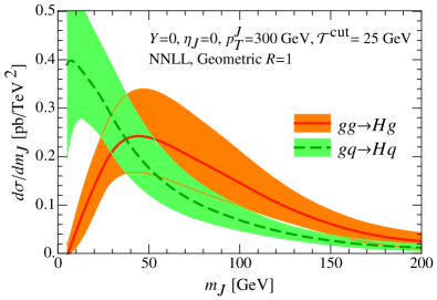
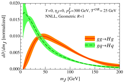
In this section we focus on the individual quark and gluon channels, leaving results for $pp\to H+1$ jet to be discussed in Sec. V below. We first study the theoretical predictions for the $m_{J}$ spectrum with and without normalization, and show that normalizing substantially reduces the perturbative uncertainty. We also study the order-by-order convergence of this differential cross section, and the size of various contributions to the perturbative uncertainty bands. Next, the dependence on the jet veto $\mathcal{T}^{\mathrm{cut}}$ is studied. Finally, we investigate the size of non-global logarithms as a function of $m_{J}$ and $\mathcal{T}^{\mathrm{cut}}$.

IV.1 Default Parameter Choices

Unless indicated otherwise we use the following default parameter choices for all plots in Secs. IV, V, and VI. For the Higgs mass we take $m_{H}=125\,\mathrm{GeV}$ :2012gk ; :2012gu , and for the LHC center-of-mass energy we take $E_{\mathrm{cm}}=7\,{\rm TeV}$. We always use the MSTW NLO PDFs Martin:2009bu with the corresponding value of $\alpha_{s}(m_{Z})=0.1202$ for the strong coupling constant. As our default we use the geometric $R=1$ measure for defining the jets, $\mathcal{T}^{\mathrm{cut}}=25\,\mathrm{GeV}$ for the jet veto, and $m_{J}^{\mathrm{cut}}=200\,\mathrm{GeV}$ for the normalization range. Our default hard kinematics are ${p_{T}^{J}}=300\,\mathrm{GeV}$, $\eta_{J}=0$, and $Y=0$. Finally, for the scale functions $\mu_{H}$, $\mu_{B_{i}}(\tau)$, $\mu_{J}(\tau)$, and $\mu_{S_{i}}(\tau)$ defined in Sec. III.3, the central parameter values are given in App. B. There we also discuss the combination of scale variations used for estimating the perturbative uncertainties.

IV.2 Normalization and Convergence

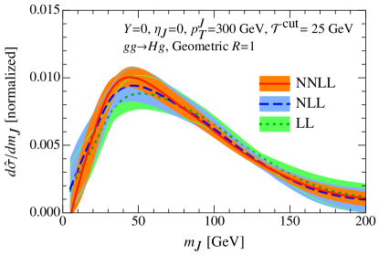
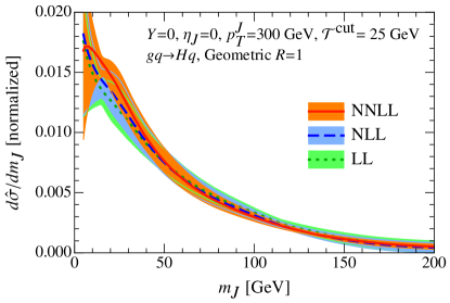
The unnormalized jet mass spectrum at NNLL with our default inputs for the quark and gluon channels are shown in Fig. 5(a). As one expects, the gluon jets peak at a much higher jet mass than the quark jets. We also see that the perturbative uncertainties are quite sizable, even at NNLL.

Figure 6: Effect of using different jet veto cuts on the jet mass spectrum for $gg\to Hg$. While the unnormalized spectrum on the left is directly sensitive to the jet veto cut, this dependence almost completely cancels in the normalized spectrum on the right. The same is true for the quark channel, $gq\to Hq$, and the sum over all partonic channels.

Normalizing the jet mass spectrum allows one to study its shape without contamination from the slow convergence of the integrated 1-jet cross section, and also reduces the experimental uncertainties significantly. We denote the normalized cross section as $\mathrm{d}\hat{\sigma}/\mathrm{d}m_{J}$ and calculate it using Eq. (19) where we normalize over the range $0\leq m_{J}\leq m_{J}^{\mathrm{cut}}$.

We first study the impact of normalization on the perturbative uncertainty. To preserve the normalization, we simultaneously vary the scales in the numerator and denominator of Eq. (19). Comparing the unnormalized cross section at NNLL for the gluon and quark channels shown in Fig. 5(a) to the normalized ones in Fig. 5(b), we observe that a substantial portion of the uncertainty is related to the integrated cross section rather than the shape. In the resummation region of the $m_{J}$ spectrum, $30\,{\rm GeV}\leq m_{J}\leq 150\,{\rm GeV}$ the normalized cross sections have a quite reasonable remaining perturbative uncertainty of $\simeq 6$–$9\%$ for gluons, and $\simeq 11$–$14\%$ for quarks.

A big part of the sizable uncertainty in the unnormalized 1-jet cross section is due to the poor convergence of the hard function for $pp\to H+1$ jet, and thus specific to the Higgs process. If we were to keep the hard function as an overall multiplicative factor it would cancel exactly in the normalized cross section for a given partonic channel and fixed phase space point. As shown by the reduction in uncertainties seen in Fig. 5(b), the majority of this cancellation still takes place despite the fact that we are using an expanded hard function as in Eq. (20). This cancellation also takes place approximately for the integrated cross section summed over partonic channels as we show below in Sec. V.2. Our results with fixed kinematics are therefore representative of results integrated over the jet phase space.

The order-by-order convergence of our resummed jet mass calculation is displayed in Figs. 5(c) and 5(d) for the gluon and quark jet channels, where results at LL, NLL, and NNLL are shown. The various bands overlap with those of lower orders, providing direct evidence that our scale variations yield a reasonable estimate of the higher-order perturbative uncertainties.

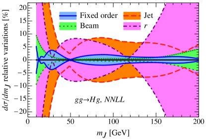
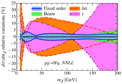
There are several classes of perturbative scale uncertainties, the “Fixed Order” scale variation that is correlated with the total cross section, the “Beam” scale variation from varying $\mu_{B_{i}}$ and $\mu_{S_{B}}$ that is related to the presence of the jet veto, the “Jet” scale variation from varying $\mu_{J}$ and $\mu_{S_{J}}$ that is related to the jet mass measurement, and the uncertainty from “r” that is related to the perturbative freedom in the refactorized formula for the soft function. For the NNLL results, these individual scale variations are shown in Figs. 5(e) and 5(f) for gluon and quark jets respectively. For simplicity we combined the uncertainty from varying the jet scale $\mu_{J}$ and the scale of the jet part of the soft function $\mu_{S_{J}}$ by taking the envelope, and similarly for the beams. It is not too surprising that the uncertainties associated with the hard and beam scale variations are smaller, since they are mostly common to the numerator and denominator of the normalized spectrum in Eq. (19). It is also not surprising that the “r” uncertainty dominates for large $m_{J}$ since in this region there is a hierarchy between $m_{J}^{2}$ and ${p_{T}^{J}}\mathcal{T}^{\mathrm{cut}}$, and the lack of resummation in this ratio shows up through this uncertainty. To obtain the total perturbative uncertainty we take the envelope of “Jet”, “Beam” and “r” uncertainties and combine it in quadrature with the “Fixed Order” uncertainty. The total uncertainty in the jet mass spectrum is dominated by that of the jet and by the soft function refactorization.

IV.3 Jet Veto and Non-Global Logarithms

Figure 7: Effect of non-global logarithms on the NNLL jet mass spectrum for $gg\to Hg$ for different jet veto cuts. Left panel: Including the leading NGLs (dashed lines) has a small effect on the unnormalized spectrum, and is well within the perturbative uncertainty for a wide range of jet veto cuts. Right panel: The effect of including the leading NGLs (black solid, dashed, and dotted curves) on the normalized NNLL spectrum (orange band) is still within the reduced perturbative uncertainty for a wide range of jet veto cuts, but start to become important for $\mathcal{T}^{\mathrm{cut}}=10\,{\rm GeV}$.

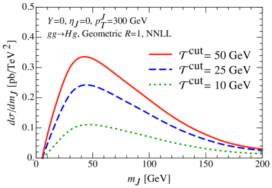
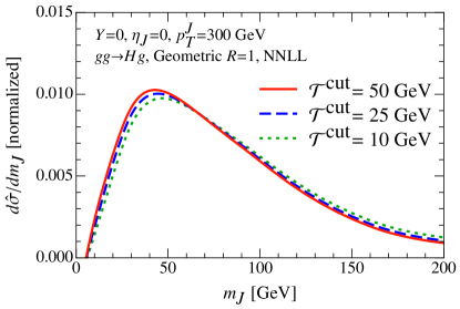
Next we discuss the effect of the jet veto on the jet mass spectrum. Our veto is imposed through the variable $\mathcal{T}^{\mathrm{cut}}$, rather than a more traditional $p_{TJ}^{\mathrm{cut}}$, since this simplifies the treatment of scales in the problem, and allows us to make use of a known factorization theorem. This jet veto restricts the initial and final-state collinear radiation as well as soft radiation. It turns out that the normalized jet mass spectrum is fairly insensitive to the value of the jet veto cut.

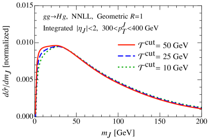
We start by considering the effect of the jet veto on the unnormalized jet mass spectrum, as shown for $gg\to Hg$ in the left panel of Fig. 6. Decreasing $\mathcal{T}^{\mathrm{cut}}$ imposes a stronger restriction on the initial-state radiation and reduces the unnormalized cross section. (This reduction is less strong for $gq\to Hq$, because quarks radiate less than gluons.) As the right panel of Fig. 6 shows, the normalization removes the majority of the $\mathcal{T}^{\mathrm{cut}}$ dependence. Note that without the refactorization of the soft function (see Sec. III.2) this cancellation would be spoiled by unphysical logarithms. This strong cancellation is also the case for the other partonic channels, as well as for their sum in $pp\to H+1$ jet. This insensitivity to $\mathcal{T}^{\mathrm{cut}}$ also remains valid after integrating over the jet phase space, as we show below in Fig. 9. We have also studied the dependence on $\mathcal{T}^{\mathrm{cut}}$ as well as a standard $p_{TJ}^{\mathrm{cut}}$ jet veto with Pythia, where we also find a similar insensitivity of the normalized jet mass spectrum to the details of the used jet-veto variable and cut values.

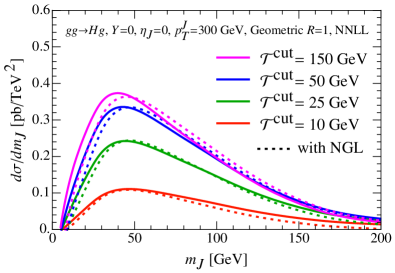
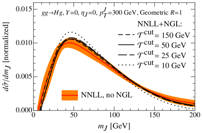
Next we turn to our analysis of NGLs, both in the unnormalized and normalized jet mass spectra. As explained in Sec. III.4, we test for the size of the NGLs by comparing the cross section with and without these terms. The leading NGL is included in fixed-order perturbation theory in the soft function, on top of which we sum an infinite series of global logarithms through the factorization formula.

In the left panel of Fig. 7 we show the unnormalized spectrum for various $\mathcal{T}^{\mathrm{cut}}$ values at NNLL (solid lines) and the same spectra including the NGL terms (dotted lines). As mentioned earlier, there is a point on the spectrum where the NGLs exactly cancel. This point is at $m_{J}\simeq 50,110,165,300$ for $\mathcal{T}^{\mathrm{cut}}=10,25,50,150\,{\rm GeV}$ respectively. For all values of $m_{J}$ shown in this figure the effect of the NGL terms is well within the perturbative uncertainty [cf. the uncertainty bands shown in Fig. 5(a)].

When we normalize the spectrum we are dividing by the cumulant with $m_{J}^{\mathrm{cut}}$, and the jet-veto dependence does not cancel out in the presence of the non-global logarithms. There are two types of NGLs in the normalized result, terms involving $\ln[m_{J}^{2}/({p_{T}^{J}}\mathcal{T}^{\mathrm{cut}})]$ from the numerator and terms involving $\ln[m_{J}^{\mathrm{cut}\,2}/({p_{T}^{J}}\mathcal{T}^{\mathrm{cut}})]$ from the denominator. Therefore for a fixed $\mathcal{T}^{\mathrm{cut}}$ there is no longer a value of $m_{J}$ where all the NGLs will vanish. Results for the normalized spectrum with and without NGLs are shown in the right panel of Fig. 7. The orange band shows the NNLL result without NGLs along with its perturbative uncertainty, while the various black lines show the central values for NNLL results that have the NGLs included. For the wide range of values $25\,{\rm GeV}\leq\mathcal{T}^{\mathrm{cut}}\leq 150\,{\rm GeV}$ the effect of the NGLs is of the same size as the reduced perturbative uncertainty in the normalized spectrum. This justifies our assertion that the NGLs do not have to be considered as large logarithms for a significant range of cut values, so that our NNLL result is complete at this order. In the small $m_{J}$ region of the spectrum the resummation of global logarithms on top of the NGL term provides an appropriate Sudakov suppression in the the cross section. For other $m_{J}$ values, and $25\,{\rm GeV}\leq\mathcal{T}^{\mathrm{cut}}\leq 150\,{\rm GeV}$, the argument of the NGL remains between $1/8$ and $8$, which is the range over which we expect that the NGLs do not dominate over nonlogarithmic corrections, as mentioned in the introduction. On the other hand, for $\mathcal{T}^{\mathrm{cut}}=10\,{\rm GeV}$ one observes that the NGLs become large enough that they are no longer contained within the perturbative uncertainty, so this value is outside the range of validity of our normalized NNLL results (though for this value the unnormalized results remain valid). For $\mathcal{T}^{\mathrm{cut}}=10\,{\rm GeV}$ the argument of the NGL involving $m_{J}^{\mathrm{cut}}$ becomes $\simeq 13$, which is outside of the range mentioned above.

Although we have only explored the $gg\to Hg$ channel at a fixed kinematic point in this section, we have also checked explicitly that the same conclusions about NGLs hold when integrating over a kinematic range, and when considering quark jets from $gq\to Hq$.

V Results for $pp\to H+1$ jet

In this section we show results for the $pp\to H+1$ jet cross section at NNLL, summing the contributions from the various partonic channels: $gg\to Hg$, $gq\to Hq$, and the (small) $q\bar{q}\to Hg$. We present results for the dependence of the jet mass spectrum on the jet kinematics, on the choice of jet definition which affects the shape of the jets, and on the jet size $R$. We also compare the $m_{J}$ spectrum obtained for a fixed point in the jet kinematics to that obtained from integrating over a range of jet momenta.

(a) The cross section decreases with increasing ${p_{T}^{J}}$.

(b) For $pp\to H+1$ jet the peak position remains stable and the spectrum slightly broadens with increasing ${p_{T}^{J}}$.

(c) The cross section decreases with increasing $\eta_{J}$.

(d) For $pp\to H+1$ jet the peak position shifts slightly and the spectrum slightly broadens with increasing $\eta_{J}$.

(e) The cross section quickly decreases for larger $Y$.

(f) For $pp\to H+1$ jet the peak position remains stable and the spectrum slightly broadens with increasing $Y$.

Figure 8: Dependence on the kinematic variables $p_{T}^{J}$, $\eta_{J}$, and $Y$ for the unnormalized and normalized NNLL jet mass spectra for $pp\to H+1$ jet.

Figure 9: Results for the normalized jet mass spectrum at NNLL for $pp\to H+1$ jet after integrating over $300\,{\rm GeV}<{p_{T}^{J}}<400\,{\rm GeV}$, $|\eta_{J}|<2$, and all $Y$. The left panel compares the spectrum for integrated kinematics (dashed line) to those for fixed kinematics with $Y=\eta_{J}=0$ and ${p_{T}^{J}}=300,360,400\,{\rm GeV}$ (solid lines from top to bottom at the peak). The right panel shows the impact of ${\cal T}^{\mathrm{cut}}$ on the normalized spectrum for integrated kinematics, which is the analog of the comparison in the right panel of Fig. 6 for fixed kinematics.

V.1 Dependence on Kinematics

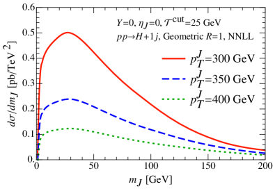
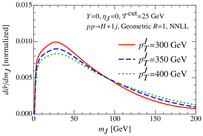
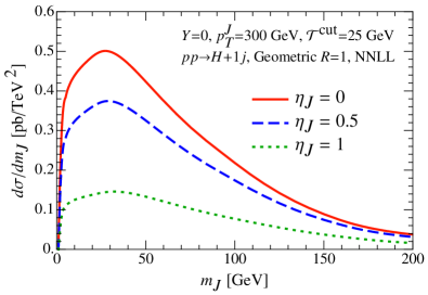
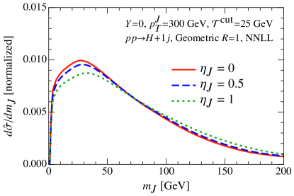
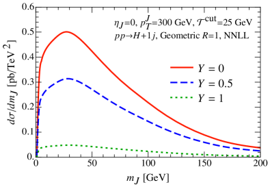
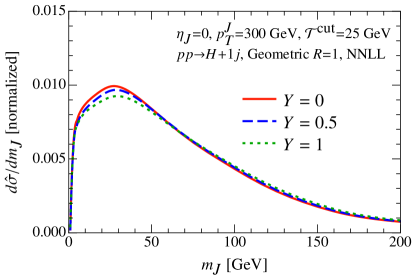
For $pp\to H+1$ jet there are three nontrivial kinematic variables: the transverse momentum of the jet $p_{T}^{J}$, rapidity of the jet $\eta_{J}$, and the total rapidity $Y$ of the combined Higgs+jet system. We show how each of these variables affect both the unnormalized and normalized jet mass spectrum, which allows us to separate the impact of kinematics on the normalization and the shape.

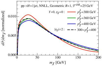
The falloff of the PDFs at larger $x$ values causes the cross section to strongly decrease for increasing ${p_{T}^{J}}$ and for increasing $|\eta_{J}|$ (for $Y=0$). This is shown in Figs. 8(a) and 8(c). The dependence on ${p_{T}^{J}}$ and $\eta_{J}$ in the corresponding normalized spectra are shown in Figs. 8(b) and 8(d). Here we see that there is a decrease in the height of the peak and a compensating increase in the tail height as ${p_{T}^{J}}$ or $|\eta_{J}|$ are increased. Note that for these variables there is a marked difference between the total $pp\to H+1$ jet process compared to the individual partonic channels (which are not shown). For each partonic channel the peak position of the jet mass spectrum increases as $m_{J}^{\rm peak}\propto\sqrt{\smash{{p_{T}^{J}}}\vphantom{p_{T}}\rule[8.61108pt]{0.0pt}{0.0pt}}$ and also increases with increasing $|\eta_{J}|$. However, at the same time the contribution of $gq\to Hq$ relative to $gg\to Hg$ is enhanced, and the peak of the jet mass spectrum is at lower values for quark jets than for gluon jets [see Fig. 5(b)]. These two effects largely cancel for $pp\to H+1$ jet, such that the peak position is practically unchanged with increasing ${p_{T}^{J}}$, whereas for increasing $\eta_{J}$ a small net increase in the peak position remains.

Note that our ability to calculate the $\eta_{J}$ dependence implies that it is trivial to impose rapidity cuts in our framework. This is an advantage of calculating the jet mass spectrum for an exclusive jet sample, where the jet veto controls radiation in the out-of-jet region.

The main dependence on the total system rapidity $Y$ enters through the shape of the PDFs, causing the cross section to strongly decrease with increasing $|Y|$, as Fig. 8(e) shows. (This is also the reason for taking central jets with $Y=0$ for our default value when using a single phase space point.) The value of $Y$ also affects the shape of the jet mass spectrum, as can be seen in Fig. 8(f). The jet rapidity relative to the partonic center of mass is $\eta_{J}-Y$, so one would expect the shape change as function of $Y$ to be similar to that as function of $\eta_{J}$, shown in Fig. 8(d). The agreement is close but not exact because the $Y$ dependence induced by the shape of the PDFs differs channel by channel, and thus affects their relative weight in the sum over channels.

V.2 Integrated Kinematics

So far we have shown the $m_{J}$ spectra for a fixed point in ${p_{T}^{J}}$, $\eta_{J}$, and $Y$. We now consider the impact of integrating the kinematic variables over a bin with $|\eta_{J}|<2$, $300\,{\rm GeV}<{p_{T}^{J}}<400\,{\rm GeV}$, and any $Y$. These kinematic ranges are realistic experimentally for jets at the LHC.

In the left panel of Fig. 9 the jet mass spectrum for integrated kinematics is shown by a black dashed line, and is compared to three spectra with fixed kinematics shown by solid lines (with $Y=\eta_{J}=0$ and ${p_{T}^{J}}=300,360,400\,{\rm GeV}$ from top to bottom at the peak of the spectrum). One observes that the $m_{J}$ spectrum in the integrated bin is very close to the $m_{J}$ spectrum with $Y=\eta_{J}=0$ and near the center of the ${p_{T}^{J}}$ bin. Thus our conclusions made from studies of a single kinematic point directly carry over to the results obtained by integrating over a phase space bin.

The one situation where this is not immediately obvious is the dependence of the normalized cross section on the jet-veto cut, ${\cal T}^{\mathrm{cut}}$, shown for fixed kinematics in Fig. 6. When we integrate over the kinematic bin the hard function, including its Sudakov form factor depending on ${\cal T}^{\mathrm{cut}}$, no longer exactly cancels between the numerator and denominator. Nevertheless, comparing the spectra for integrated kinematics and different values of ${\cal T}^{\mathrm{cut}}$, shown in Fig. 9, we see that the normalized spectrum is still very insensitive to the details of the jet veto also after summing over partonic channels and integrating over a range of kinematics. (We have also confirmed that upon phase space integration the size of the NGL effect remains the same as shown in Fig. 7.)

V.3 Jet Definitions and Jet Area

Figure 10: Dependence of the NNLL jet mass spectrum for $pp\to H+1$ jet on the $N$-jettiness measure used to define the jets.

Figure 11: Dependence of the NNLL jet mass spectrum for the geometric $R$ measure on the jet radius $R$. Only the $R$ dependence from singular terms in the factorization formula is shown here.

In Sec. II we discussed the various $N$-jettiness measures (defined by the $Q_{i}$) and illustrated the corresponding size and shape of the jet regions for the geometric cases. An illustration of the more irregular regions that appear for the invariant mass measure can be found in Ref. Jouttenus:2011wh . We now study how the jet mass spectrum is affected by these different jet definitions as well as by their jet area ($R$ dependence). We start by noting that in the $N$-jettiness factorization only the soft function is sensitive to the boundaries of the jet regions. Up to NLL the only jet algorithm dependence enters through the arguments of the logarithms, such as $\ln[m_{J}^{2}/(Q_{J}{p_{T}^{J}})]$. More complicated dependence on the boundaries enters through the soft function starting at NLO, which appears in our NNLL results. The nontrivial jet radius and jet algorithm dependence in the singular terms in the factorization theorem is formally enhanced for $m_{J}\ll{p_{T}^{J}}$ over the dependence on the jet algorithm and jet area in the power-suppressed nonsingular terms that are not part of Eq. (III.2).

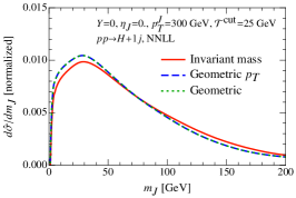
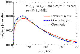
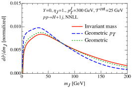
In Fig. 10 we compare the invariant mass, geometric $p_{T}$, and geometric measures for three different kinematic configurations with $\eta_{J}=\{0,0.5,1\}$, $Y=0$, and $p_{T}^{J}=300$ GeV. We fix $\rho=0.834$ for the two geometric measures (which corresponds to $R=1$ for the geometric measure at $\eta_{J}=0$). When increasing $\eta_{J}$, all three measures show a mild decrease in the peak height and mild increase in the tail. For $\eta_{J}=0$ the dependence of the jet mass on the jet definition is quite mild (for jets of similar area): the invariant mass measure is very similar to the geometric measures, and the two geometric measures agree exactly as we saw already in Fig. 1(a). For more forward jet rapidities the two geometric measures start to progressively differ, with the geometric measure being closer to the invariant mass result.

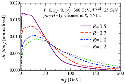
In Fig. 11 we show the jet mass spectrum for the geometric $R$ measure for various values of the jet radius $R$. A smaller jet radius translates into a higher peak and shorter tail. (The small bump at the top of the $R=0.5$ peak is not significant within our uncertainties.) Indeed, one of the most significant effects on the jet mass spectra for different values of $R$ is the fact that the size of the jet puts an effective upper boundary on its mass $m_{J}\lesssim p_{T}^{J}R/\sqrt{2}$. At this boundary the jet mass spectrum has to fall off rapidly. This boundary is seen in Pythia and LHC data and is incorporated into our resummation by determining the point where we transition from the resummation region to the fixed-order region. Since this decreases the size of the tail of the jet mass spectrum there must be a corresponding increase to the peak to ensure the result remains normalized. Note that the precise form of the jet mass spectrum near $m_{J}\sim p_{T}^{J}R/\sqrt{2}$ is not fully predicted by our calculation, because we have not yet incorporated the nonsingular contributions to the cross section. These are important for making accurate predictions in this part of the tail of the distribution, where their size is not fully captured by our perturbative uncertainty estimates.

VI Monte Carlo Comparisons

In this section we study various aspects of the jet mass spectrum in Pythia. Although formally the perturbative accuracy of Pythia is significantly lower than that of our NNLL calculation, it is also well known that after sufficient tuning Pythia is able to reproduce the shape of many jet observables. Here we are particularly interested in testing the impact on the jet mass spectrum from using different hard processes, using different jet algorithms, and from adding hadronization and underlying event (the latter being described by Pythia’s multi-parton interaction model). We also perform a comparison between our calculation and Pythia for the same geometric $R=1$ $N$-jettiness jets used in our analysis. Finally we compare our exclusive 1-jet $m_{J}$ calculation with the inclusive jet mass spectrum measured in $pp\to$ jets by ATLAS. We always use Pythia8 with its default tune 5 (“Tune 4C”), which as we will see provides a good description of the ATLAS jet mass data.

VI.1 Hard Process and Jet Algorithm Dependence in PYTHIA

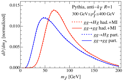
We start by investigating to what extent the jet mass spectrum depends on the underlying hard process in Pythia. In Fig. 12 we show the spectrum for a gluon jet from $gg\to gg$ (solid) and from $gg\to Hg$ (dotted), demonstrating that in Pythia there is essentially negligible process dependence for individual partonic channels. This is true both at the partonic level (blue curves with peak on the left) and after including hadronization and multiple interactions (red curves with peak on the right). In reality one expects some differences from the hard process due to the additional soft radiation produced with more available colored particles, and from the different color flow, where in particular $gg\to gg$ involves a matrix of color channels with nontrivial interference. These effects may not be sufficiently described by Pythia so one should not conclude that the hard process dependence on the jet mass spectrum is as small as is shown.

Figure 12: The gluon jet mass spectrum in Pythia does not depend on the underlying hard process producing the jets. This is true both for partons (left peaks) and with hadronization and underlying event (right peaks).

Figure 13: Comparison of the normalized jet mass spectra for exclusive and inclusive jet samples in Pythia.

Figure 14: Comparison of the anti-$k_{T}$, CA, and geometric $R$ jet algorithms in Pythia.

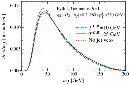
Next, we look at the difference in Pythia between the jet mass for exclusive and inclusive jet production. We use the process $gg\to Hg$, imposing the jet veto $\mathcal{T}^{\mathrm{cut}}=10,25$ GeV to obtain two exclusive samples, and using no jet veto for our inclusive sample. The resulting normalized jet mass spectra are shown in Fig. 13. The difference between $\mathcal{T}^{\mathrm{cut}}=25$ GeV (our default value) and the inclusive case is small, allowing our calculation to be compared to inclusive spectra. The difference is slightly larger for $\mathcal{T}^{\mathrm{cut}}=10$ GeV and increases significantly for smaller values of $\mathcal{T}^{\mathrm{cut}}$. However, we will not consider such strong jet vetos, as they lead to large NGLs (see Sec. IV.3).

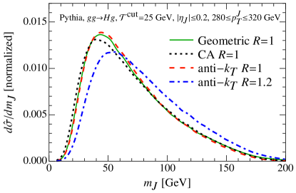
In Fig. 14 we compare the jet mass spectrum from Pythia for different jet algorithms, specifically our 1-jettiness $R=1$-algorithm, Cambridge-Aachen with $R=1$, and anti-k_T with $R=1$ and $R=1.2$ Cacciari:2011ma . To stay close to a calculation for a single phase space point, we restrict the jet to a narrow $p_{T}$ and rapidity bin, and impose a veto using $\mathcal{T}^{\mathrm{cut}}=25$ GeV. The differences between the $R=1$ curves are within the size of the uncertainty band from our NNLL calculation in the same phase space bin. This result agrees with the small differences observed in each of the panels of Fig. 10 from comparing different jet measures for 1-jettiness jets. The difference between $R=1$ and $R=1.2$ for anti-k_T is a bit larger than that observed in our calculation using geometric $R$ jets in Fig. 11. In Pythia the difference between $R=1$ and $R=1.2$ becomes smaller when $\mathcal{T}^{\mathrm{cut}}$ is decreased, since with a stronger jet veto less additional radiation is present that would be absorbed by larger jets. To be specific, the 15% difference in the peak heights for anti-k_T with $R=1$ and $R=1.2$ for $\mathcal{T}^{\mathrm{cut}}=25$ GeV reduces to 7% for $\mathcal{T}^{\mathrm{cut}}=5$ GeV.

VI.2 Comparison of NNLL with PYTHIA

A comparison between our NNLL calculation and partonic Pythia results for $gg\to Hg$ are shown in the two panels of Fig. 15.

Figure 15: Comparison between our NNLL calculation and partonic Pythia for the $gg\to Hg$ channel. Both results use geometric $R=1$ jets and the same kinematic cuts.

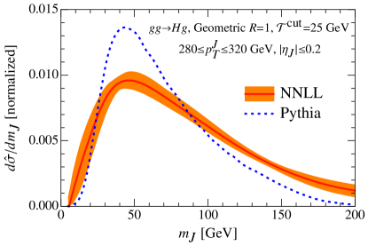
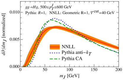
In the top panel of Fig. 15 we show results for a narrow ${p_{T}^{J}}$ bin about ${p_{T}^{J}}=300\,{\rm GeV}$ and use the geometric $R=1$ jet definition for both Pythia and the NNLL results. The peak positions in both cases agree very well. To ensure that this is not an accident and that the peak position in Pythia does not depend on the PDF set used by our default tune, we checked that an alternative tune (number 10, which is based on our default Pythia tune but uses MSTW2008 LO PDFs) only shifts the peak by a small amount, similar to the small difference in peak positions between Pythia and our NNLL calculation. However, as seen in Fig. 15, the NNLL calculation has a somewhat lower peak and a correspondingly higher tail. Since the spectrum is normalized these two effects are related, namely higher values in the tail must be compensated by a lower peak. There are several possibilities that may account for this difference. Due to the stability of our order-by-order results in Fig. 5(c) it is unlikely to be related to the lower order accuracy of Pythia’s LL parton shower resummation. Most likely the differences are related to the fact that we have not yet included nonsingular contributions to the spectrum which are important in the fixed-order region, in particular for the spectrum to fall off rapidly enough. Due to the fact that the results are normalized, this mismatch in the tail then also leads to a disagreement of the peak heights. Thus we expect that the inclusion of the nonsingular contributions will reduce this difference. Note that an estimate for the size of these nonsingular terms is not included in our perturbative uncertainty bands.

In the bottom panel of Fig. 15 we compare results at larger ${p_{T}^{J}}$ bin, $500\leq{p_{T}^{J}}\leq 600\,{\rm GeV}$, again normalizing both the Pythia and NNLL results over the same $m_{J}=0$–$200\,{\rm GeV}$ range. For a common jet radius $R=1$ there is mild dependence on the jet algorithm as explored earlier, and we show the Pythia results for anti-$k_{T}$ and CA. Here there is an improved agreement between our NNLL results and Pythia, with the largest effect again being the higher tail.

VI.3 Hadronization in PYTHIA

Figure 16: The nonperturbative hadronization correction in Pythia is well described by a shift in $m_{J}^{2}$.

Figure 17: Comparison of the Pythia jet mass spectrum for inclusive $pp\to$ jets to the corresponding ATLAS data ATLAS:2012am . Pythia results are shown at parton level (dotted), including hadronization (dashed), and including hadronization and multiple interactions (solid). The final Pythia results reproduce the data well.

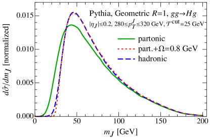
We now explore the effect of hadronization on the jet mass spectrum using Pythia. In the factorization formula the hadronization is encoded through nonperturbative corrections in the soft function $S$ at a scale $\sim\Lambda_{\rm QCD}$, which must be separated from perturbative corrections at the soft scale $\mu_{S}\sim m_{J}^{2}/{p_{T}^{J}}$. For $e^{+}e^{-}\!\to 2$ jets there is an analytic understanding of the analogous nonperturbative corrections originating in Refs. Dokshitzer:1995qm ; Dokshitzer:1995zt ; Dokshitzer:1997iz ; Salam:2001bd as well as a modern understanding in terms of field theory operators Korchemsky:1999kt ; Lee:2006fn ; Hoang:2007vb ; Mateu:2012nk . For these processes, as soon as the relevant soft scale $\mu_{S}$ is perturbative, the nonperturbative corrections can be power expanded in $\Lambda_{\rm QCD}/\mu_{S}$, and the dominant power correction simply shifts the event shape distribution, $e\to e-\Omega_{e}/Q$. In the case at hand, the nonperturbative soft function is built from more than two Wilson lines, so the description of the power corrections becomes more complicated. Nevertheless, for a given kinematic configuration we still expect that the dominant effect will be described by a shift involving a parameter $\Omega\sim\Lambda_{\rm QCD}$. For a jet mass $m_{J}^{2}\simeq p_{J}^{+}p_{J}^{-}$ this shift occurs due to nonperturbative soft radiation causing a shift in the small momentum $p_{J}^{+}$, so it takes the form

$$m_{J}^{2}\to m_{J}^{2}-2\Omega\,p_{T}^{J}\,R\,.$$ (39)

The factor of $R$ accounts for the fact that there is a decreased amount of soft momentum contamination in the jet for decreasing $R$ Dasgupta:2007wa . It is straightforward to test whether this shift agrees with the hadronization model in Pythia, by comparing the results with and without hadronization. As demonstrated in Fig. 16, a shift with the choice $\Omega=0.8$ GeV works very well, in reasonable agreement with the $\Omega=1.0$ GeV found earlier in Ref. Dasgupta:2012hg for the inclusive $\geq 1$ jet cross section.

Figure 18: Comparison of our exclusive NNLL calculation with ATLAS inclusive jet mass data ATLAS:2012am . The peak position of our gluon jets from $gg\to Hg$ agrees remarkably well with the inclusive dijet data. For the ATLAS date there is presumably a shift to lower values due to quark jets which is compensated by a shift to higher values due to hadronization and multiple interactions.

VI.4 Underlying Event and ATLAS Data

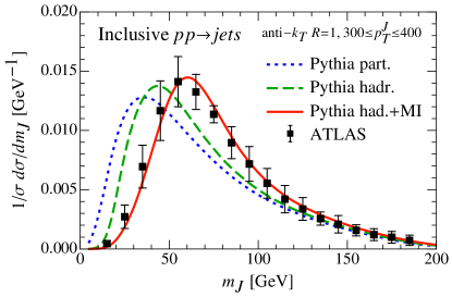
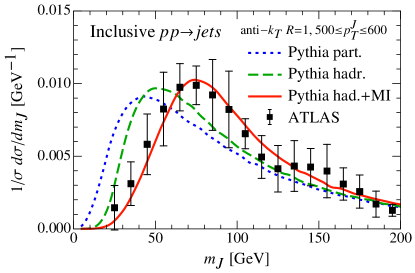
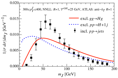
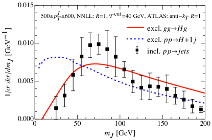
In Pythia the effect of the underlying event is modeled by multiple partonic interactions, and its effect on the jet mass spectrum is more pronounced than that of hadronization. This is shown in Fig. 17 where we plot the jet mass spectrum for inclusive $pp\to$ jets from Pythia at parton level, including hadronization, and including hadronization and multiple interactions. Also shown are the corresponding ATLAS data from Ref. ATLAS:2012am , where the uncertainty bars are from linearly combining the statistical and systematic uncertainties. This channel is dominated by the copious $pp\to$ dijet production at the LHC. We use the same inputs and cuts as ATLAS, namely $E_{\mathrm{cm}}=7\,{\rm TeV}$, anti-k_T jets with $R=1$, $|\eta_{J}|\leq 2$, and consider both $300\,{\rm GeV}\leq{p_{T}^{J}}\leq 400\,{\rm GeV}$ and $500\,{\rm GeV}\leq{p_{T}^{J}}\leq 600\,{\rm GeV}$. The shift to the peak location from hadronization is of similar magnitude as that for $gg\to Hg$ in Fig. 16, namely $\simeq 3.0\,{\rm GeV}$ for $gg\to Hg$ compared to $\simeq 8.0\,{\rm GeV}$ for the $300\,{\rm GeV}\leq{p_{T}^{J}}\leq 400\,{\rm GeV}$ inclusive jets which have a slightly larger average ${p_{T}^{J}}$. For the inclusive $pp\to$ jets in Pythia the additional shift to the peak location from the underlying event is $\simeq 17.4\,{\rm GeV}$. The final Pythia results agree well with the ATLAS data for both ${p_{T}^{J}}$ bins. In a NNLL calculation the effect of hadronization and part of the effect of the underlying event will be captured by corrections to the soft function, but it is not clear if hadronic corrections in the multi-jet soft function will fully capture the effect of the underlying event.

Given that Pythia agrees well with the ATLAS inclusive dijet spectrum, one might wonder what the purpose of a higher-order NNLL dijet calculation would be. An advantage of our calculational framework over Pythia is that it follows from first principles and does not involve the modeling and tuning present in Pythia. Specifically, the input to our calculation is limited to $\alpha_{s}(m_{Z})$, the parton distributions functions, and simple soft function parameters like $\Omega$ for the hadronic effects. Furthermore, we have a rigorous estimate of the higher-order perturbative uncertainty from scale variation, as well as from order-by-order convergence, which enable us to fully assess the reliability of the result. Finally, it should be emphasized that our calculation is fully analytic (up to the numerical convolution with the PDFs) and hence provides an analytic QCD calculation of an LHC spectrum for jets.

To the extent that the normalized jet mass spectrum is independent of the hard process and independent of using an inclusive or exclusive jet sample, which Pythia seems to suggest in Figs. 12 and 13, a comparison between jet mass spectra involving different hard processes and with and without jet veto cuts is appropriate. The approximate hard process independence only holds separately for gluon or quark jets, which themselves have fairly different jet mass spectra, see Fig. 5(b). Therefore when varying the hard process we expect the dominant change in the jet mass spectrum to be related to the process dependent fraction of quark and gluon jets produced.

In Fig. 18 we compare our NNLL result for $pp\to H+1$ jet and for $gg\to Hg$ to the ATLAS data for $pp\to$ jets. Recall that the peak location of the NNLL $H+1$ jet calculation matches well with that from Pythia, see Fig. 15. Because of the significant contribution from quark jets the $H+1$ jet spectrum peaks to the left of the spectrum from dijets. On the other hand, the peak location with pure gluon jets ($gg\to Hg$) agrees quite well with the data on dijets, particularly for the larger ${p_{T}^{J}}$ bin. From the results already obtained above, we expect only small differences (comparable to the ATLAS error bars) for effects related to the choice of the jet algorithm, the choice of inclusive versus exclusive jets, or the choice of looking at gluon jets in dijets or in Higgs production. On the other hand there will be a more significant shift of the spectrum to the left from quark channels in the dijet production, and a shift to the right from adding hadronization and underlying event, neither of which is included in the solid red curve. The agreement between peak locations seems to indicate that these two effects largely compensate for one another. Finally, there will be an effect related to the fact that there are nontrivial color correlations in $gg\to gg$ which are not present in $gg\to Hg$ (these effects are not apparent in Pythia, see Fig. 12).

One may also look at the peak heights in Fig. 18, for which the agreement is not as good. As described earlier, this effect is related to the fact that we have not yet included nonsingular corrections. These corrections are known to decrease the tail to enable it to rapidly fall off by $m_{J}^{2}\sim{p_{T}^{J\,2}}R^{2}/2$, and they also affect the peak directly through the normalization. Since with additional work these can be included in future results the difference in peak heights is not of too much concern.

Finally one may also compare the results in Figs. 17 and 18 for the $300\,{\rm GeV}\leq{p_{T}^{J}}\leq 400\,{\rm GeV}$ and $500\,{\rm GeV}\leq{p_{T}^{J}}\leq 600\,{\rm GeV}$ bins. For dijets the peak location moves to higher $m_{J}$ with increased ${p_{T}^{J}}$, unlike for $pp\to H+1$ jet, again indicating that gluon jets likely dominate. The conclusions from the comparison with Pythia and the contrast to our NNLL calculation remains the same for these two ranges of ${p_{T}^{J}}$.

VII Conclusions

In this paper we calculated the jet mass spectrum for $pp\to H+1$ jet to NNLL order. For this exclusive 1-jet cross section we veto additional jets with the 1-jettiness event shape, and used the 1-jettiness factorization formula in terms of hard, beam, jet, and soft functions to obtain our results. For the normalized jet mass spectrum the remaining higher-order perturbative uncertainties from scale variation are at the $\simeq 6-14\%$ level at NNLL order, being on the smaller side of this range for gluon jets. In addition, our results exhibit excellent order-by-order convergence.

The normalized NNLL spectrum is quite insensitive to the jet veto over a wide range of values, even when accounting for non-global logarithms. Thus in our framework non-global logarithms can be accurately treated as fixed-order contributions to the soft function, upon which additional global logarithms are automatically resummed in the factorization framework. An essential ingredient in the resummation of the global logarithms was the refactorization of the soft function, which we demonstrate is required to avoid introducing spurious leading logarithms in certain regions of phase space. Our treatment of the NNLL exclusive cross section with a jet veto has significantly smaller non-global logarithmic terms when compared to the size of these terms observed in the earlier inclusive NLL analysis in Ref. Banfi:2010pa , and the earlier inclusive partial NNLL analysis in Ref. Kelley:2012kj . Finally, we note that in Pythia the inclusive jet mass spectrum and the exclusive jet mass spectrum with our default jet veto are essentially identical.

Utilizing our calculation we investigated the dependence of the jet mass spectrum on various parameters of the exclusive jet cross section. Part of the power of our framework is that the factorization formula is fully differential in the jet kinematics (${p_{T}^{J}}$, $\eta_{J}$, and $Y$), allowing us to vary the definition of the jets and the jet area, and can be easily separated into quark jet and gluon jet channels. As expected we find that the spectrum peaks at larger $m_{J}$ values for gluon jets than for quark jets. For a given partonic channel the factorization framework predicts little sensitivity to the underlying hard process, and this result is also found to be the case in Pythia. The main process dependence is therefore the relative mix of quark and gluon jets. The peak of our NNLL $m_{J}$ spectrum moves to the right for larger ${p_{T}^{J}}$ and for larger $|\eta_{J}|$, but more so for the individual partonic channels than for $pp\to H+$1 jet, where the change to the mix of quarks and gluons provides a compensating effect. The complete description of the various kinematic variables also makes it trivial to implement rapidity cuts. For a bin $|\eta_{J}|<2$ and a not too large bin in ${p_{T}^{J}}$, we find that the integrated NNLL result is very consistent with the NNLL result for fixed kinematic variables taken at the center of the bin.

Varying the jet definition with fixed jet area leads to small changes in the jet mass spectrum, both for various jet definitions in our NNLL result and for anti-$k_{T}$, CA, and geometric-$R$ jets in Pythia. This suggests that there are only small differences between the spectrum for 1-jettiness jets and traditional jet algorithms. On the other hand, both Pythia and our NNLL results exhibit a larger dependence on the jet radius $R$. In the fixed-order region near the jet boundary $m_{J}\sim{p_{T}^{J}}R/\sqrt{2}$ there are nonsingular terms that become important that have not been included in our analysis here. The absence of these terms likely leads to a larger tail in our NNLL spectrum than in Pythia, and correspondingly a smaller peak height in the normalized NNLL result. On the other hand, the peak location agrees very well between our NNLL calculation and Pythia. An analysis of these additional nonsingular terms will be carried out in the future.

We investigated the dependence of the jet mass spectrum on hadronization and underlying event using Pythia. Hadronization is very well described by a shift to the mass spectrum, $m_{J}^{2}\to m_{J}^{2}-(2R{p_{T}^{J}})\Omega$ with $\Omega\sim\Lambda_{\rm QCD}$, which is the anticipated result from nonperturbative soft gluon contributions in our factorization formula’s soft function. In Pythia the underlying event is modeled by multiple partonic interactions and leads to a somewhat larger shift to the spectrum than for hadronization. It plays an important role in obtaining agreement with the ATLAS jet mass results for inclusive dijets. Comparing our results to ATLAS we find that the NNLL $pp\to H+$1 jet spectrum peaks to the left of the dijet data, whereas the NNLL $gg\to Hg$ spectrum peaks in the same location. The comparison made so far with the ATLAS data is promising. The extension of our NNLL calculation to $pp\to$ dijets is completely feasible using 2-jettiness, and it will be interesting to see to what extent the contributions from quark channels, color mixing, and hadronization and underlying event will affect this comparison with the data. Theoretically, the only remaining challenge to a complete comparison appears to be incorporating the effect of the underlying event from first principles rather than relying on its modeling via Monte Carlo.

Appendix A Perturbative Inputs

In this section we collect the fixed-order ingredients and evolution kernels for evaluating the jet mass cross section for $pp\to H+1j$ in Eqs. (III.1) and (III.2) at NNLL order. We first give expressions for the hard, jet, beam and soft functions at next-to-leading order. This is followed by the evolution kernels and the coefficients that they depend on.

A.1 Hard Function

The hard functions $H_{\kappa}$ for the various partonic channels $\kappa$ that contribute to $pp\to H+1$ jet can be obtained from the finite part of the helicity amplitudes $A$ determined in Ref. Schmidt:1997wr following the procedure of Ref. Stewart:2012yh ,

$$H_{ggg}(\{q_{i}^{\mu}\},\mu_{H}) =\frac{16\alpha_{s}(\mu_{H})^{3}C_{A}^{2}C_{F}}{9\pi v^{2}}\frac{1}{[2(N_{c}^{2}-1)]^{2}}\Big{[}|A(1_{g}^{+},2_{g}^{+},3_{g}^{+};4_{H})|^{2}+|A(1_{g}^{+},2_{g}^{+},3_{g}^{-};4_{H})|^{2}$$

$$\quad+|A(1_{g}^{+},3_{g}^{+},2_{g}^{-};4_{H})|^{2}+|A(3_{g}^{+},2_{g}^{+},1_{g}^{-};4_{H})|^{2}\Big{]}\,,$$

$$H_{g{\bar{q}}{\bar{q}}}(\{q_{i}^{\mu}\},\mu_{H}) =\frac{8\alpha_{s}(\mu_{H})^{3}C_{A}C_{F}}{9\pi v^{2}}\frac{1}{2N_{c}}\frac{1}{2(N_{c}^{2}-1)}\Big{[}|A(1_{g}^{+},2_{q}^{+},3_{\bar{q}}^{-};4_{H})|^{2}+|A(1_{g}^{-},2_{q}^{+},3_{\bar{q}}^{-};4_{H})|^{2}\Big{]}\,,$$

$$H_{\bar{q}g\bar{q}}(\{q_{i}^{\mu}\},\mu_{H}) =\frac{8\alpha_{s}(\mu_{H})^{3}C_{A}C_{F}}{9\pi v^{2}}\frac{1}{2N_{c}}\frac{1}{2(N_{c}^{2}-1)}\Big{[}|A(2_{g}^{+},1_{q}^{+},3_{\bar{q}}^{-};4_{H})|^{2}+|A(2_{g}^{-},1_{q}^{+},3_{\bar{q}}^{-};4_{H})|^{2}\Big{]}\,,$$

$$H_{q{\bar{q}}g}(\{q_{i}^{\mu}\},\mu_{H}) =\frac{8\alpha_{s}(\mu_{H})^{3}C_{A}C_{F}}{9\pi v^{2}}\frac{1}{(2N_{c})^{2}}\Big{[}|A(3_{g}^{+},2_{q}^{+},1_{\bar{q}}^{-};4_{H})|^{2}+|A(3_{g}^{-},2_{q}^{+},1_{\bar{q}}^{-};4_{H})|^{2}\Big{]}\,,$$

$$H_{gqq}(\{q_{i}^{\mu}\},\mu_{H}) =H_{g{\bar{q}}{\bar{q}}}(\{q_{i}^{\mu}\},\mu_{H})\,,\qquad H_{qgq}(\{q_{i}^{\mu}\},\mu_{H})=H_{\bar{q}g\bar{q}}(\{q_{i}^{\mu}\},\mu_{H})\,,$$

$$H_{\bar{q}qg}(\{q_{i}^{\mu}\},\mu_{H}) =H_{q{\bar{q}}g}(\{q_{i}^{\mu}\},\mu_{H})\,.$$ (40)

The factors of $1/(2N_{c})$ and $1/[2(N_{c}^{2}-1)]$ arise from averaging over the spins and colors of the colliding quarks and gluons. The arguments of a helicity amplitude $A$ have the form $i_{t}^{h}$, where $i$ denotes the momentum $q_{i}^{\mu}$, $t$ denotes the parton type, and $h$ denotes the helicity of this particle. Only in the helicity amplitudes will we use an outgoing convention for all these quantities, to make crossing symmetry direct. This implies that if we want to convert to the convention used in the main text, then the $s_{ij}$’s in the helicity amplitudes below will pick up additional minus signs if one of the particles $i$ and $j$ is in and the other is out. The amplitudes that enter in Eq. (A.1) are given by

$$A(1_{g}^{+},2_{g}^{+},3_{g}^{+};4_{H}) =\frac{m_{H}^{4}}{\sqrt{2|s_{12}s_{13}s_{23}|}}\biggl{\{}1\!+\!\frac{\alpha_{s}(\mu_{H})}{4\pi}\Big{[}f(s_{12},s_{13},s_{23},m_{H}^{2},\mu_{H})\!+\!\frac{1}{3}(C_{A}\!-\!2T_{F}n_{f})\,\frac{s_{12}s_{13}\!+\!s_{12}s_{23}\!+\!s_{13}s_{23}}{m_{H}^{4}}\Big{]}\biggr{\}}\,,$$

$$A(1_{g}^{+},2_{g}^{+},3_{g}^{-};4_{H}) =\frac{s_{12}^{2}}{\sqrt{2|s_{12}s_{13}s_{23}|}}\biggl{\{}1+\frac{\alpha_{s}(\mu_{H})}{4\pi}\Big{[}f(s_{12},s_{13},s_{23},m_{H}^{2},\mu_{H})+\frac{1}{3}(C_{A}-2T_{F}n_{f})\,\frac{s_{13}s_{23}}{s_{12}^{2}}\Big{]}\biggr{\}}\,,$$

$$A(1_{g}^{+};2_{q}^{+},3_{\bar{q}}^{-};4_{H}) =\frac{s_{12}}{\sqrt{2|s_{23}|}}\biggl{\{}1+\frac{\alpha_{s}(\mu_{H})}{4\pi}\Big{[}g(s_{12},s_{13},s_{23},m_{H}^{2},\mu_{H})+(C_{F}-C_{A})\,\frac{s_{23}}{s_{12}}\Big{]}\biggr{\}}\,,$$

$$A(1_{g}^{-};2_{q}^{+},3_{\bar{q}}^{-};4_{H}) =\frac{s_{13}}{\sqrt{2|s_{23}|}}\biggl{\{}1+\frac{\alpha_{s}(\mu_{H})}{4\pi}\Big{[}g(s_{12},s_{13},s_{23},m_{H}^{2},\mu_{H})+(C_{F}-C_{A})\,\frac{s_{23}}{s_{13}}\Big{]}\biggr{\}}\,,$$

$$f(s_{12},s_{13},s_{23},m_{H}^{2},\mu_{H}) =-C_{A}\biggl{[}\frac{1}{2}(L_{12}^{2}+L_{13}^{2}+L_{23}^{2})+L_{12/H}L_{13/H}+L_{12/H}L_{23/H}+L_{13/H}L_{23/H}$$

$$\quad+2\mathrm{Li}_{2}\Bigl{(}1-\frac{s_{12}}{m_{H}^{2}}\Bigr{)}+2\mathrm{Li}_{2}\Bigl{(}1-\frac{s_{13}}{m_{H}^{2}}\Bigr{)}+2\mathrm{Li}_{2}\Bigl{(}1-\frac{s_{23}}{m_{H}^{2}}\Bigr{)}-5-\frac{3\pi^{2}}{4}\biggr{]}-3C_{F}\,,$$

$$g(s_{12},s_{13},s_{23},m_{H}^{2},\mu_{H}) =C_{A}\biggl{[}-\frac{1}{2}(L_{12}^{2}+L_{13}^{2}-L_{23}^{2})+L_{12/H}L_{13/H}-(L_{12/H}+L_{13/H})L_{23/H}-2\mathrm{Li}_{2}\Bigl{(}1-\frac{s_{23}}{m_{H}^{2}}\Bigr{)}$$

$$\quad+\frac{22}{3}+\frac{\pi^{2}}{4}\biggr{]}+C_{F}\biggl{[}-L_{23}^{2}+3L_{23}-2L_{12/H}L_{13/H}-2\mathrm{Li}_{2}\Bigl{(}1-\frac{s_{12}}{m_{H}^{2}}\Bigr{)}-2\mathrm{Li}_{2}\Bigl{(}1-\frac{s_{13}}{m_{H}^{2}}\Bigr{)}$$

$$\quad-11+\frac{\pi^{2}}{2}\biggr{]}+\beta_{0}\Bigl{(}-L_{23}+\frac{5}{3}\Bigr{)}\,.$$ (41)

Here we use the shorthand notation

$$L_{ij} =\ln\Bigl{(}-\frac{s_{ij}}{\mu_{H}^{2}}-\mathrm{i}0\Bigr{)}\,,$$

$$L_{ij/H} =\ln\Bigl{(}-\frac{s_{ij}}{\mu_{H}^{2}}-\mathrm{i}0\Bigr{)}-\ln\Bigl{(}-\frac{m_{H}^{2}}{\mu_{H}^{2}}-\mathrm{i}0\Bigr{)}\,.$$ (42)

Explicit values for the $s_{ij}$ follow once we identify $q_{i}$ and $q_{j}$ as corresponding to the jet or a beam region. In particular here

$$s_{ab} =Q^{2}\,, s_{a1} =-Q\,{p_{T}^{J}}\,e^{Y-\eta_{J}}\,, s_{b1} =-Q\,{p_{T}^{J}}\,e^{\eta_{J}-Y}\,.$$ (43)

In contrast, the convention used in the main text is $s_{ij}>0$.

A.2 Jet Functions

The one-loop jet functions are given by Bauer:2003pi ; Fleming:2003gt ; Becher:2009th

$$J_{q}(s,\mu_{J}) =\delta(s)+\frac{\alpha_{s}(\mu_{J})C_{F}}{2\pi}\Big{[}\frac{2}{\mu_{J}^{2}}{\mathcal{L}}_{1}\Big{(}\frac{s}{\mu_{J}^{2}}\Big{)}$$

$$\quad-\frac{3}{2\mu_{J}^{2}}{\mathcal{L}}_{0}\Big{(}\frac{s}{\mu_{J}^{2}}\Big{)}-\Big{(}\frac{\pi^{2}}{2}-\frac{7}{2}\Big{)}\delta(s)\Big{]}\,,$$

$$J_{g}(s,\mu_{J}) =\delta(s)+\frac{\alpha_{s}(\mu_{J})}{2\pi}\Big{\{}\frac{2C_{A}}{\mu_{J}^{2}}{\mathcal{L}}_{1}\Big{(}\frac{s}{\mu_{J}^{2}}\Big{)}-\frac{\beta_{0}}{2\mu_{J}^{2}}{\mathcal{L}}_{0}\Big{(}\frac{s}{\mu_{J}^{2}}\Big{)}$$

$$\quad+\Big{[}\Big{(}\frac{2}{3}-\frac{\pi^{2}}{2}\Big{)}C_{A}+\frac{5}{6}\beta_{0}\Big{]}\delta(s)\Big{\}}\,,$$ (44)

where the plus distributions ${\mathcal{L}}_{n}$ are defined as

$${\mathcal{L}}_{n}(x) \equiv\biggl{[}\frac{\theta(x)\ln^{n}x}{x}\biggr{]}_{+}$$ (45)

$$=\lim_{\beta\to 0}\biggl{[}\frac{\theta(x-\beta)\ln^{n}x}{x}+\delta(x-\beta)\,\frac{\ln^{n+1}\!\beta}{n+1}\biggr{]}\,.$$

The ${\cal L}_{n}(x)$ integrate to zero if the range in $x$ is $[0,1]$.

A.3 Beam Functions

The beam functions can be expressed in terms of standard gluon and quark PDFs using an operator product expansion Fleming:2006cd ; Stewart:2009yx ,

$$B_{i}(t,x,\mu_{B}) =\sum_{j=\{g,q,\bar{q}\}}\int_{x}^{1}\!\frac{\mathrm{d}\xi}{\xi}\,{\mathcal{I}}_{ij}\Bigl{(}t,\frac{x}{\xi},\mu_{B}\Bigr{)}f_{j}(\xi,\mu_{B})$$

$$\quad\times\biggl{[}1+{\mathcal{O}}\Bigl{(}\frac{\Lambda_{\mathrm{QCD}}^{2}}{t}\Bigr{)}\biggr{]}\,.$$ (46)

The one-loop matching coefficients are Stewart:2010qs ; Berger:2010xi are

$${\mathcal{I}}_{qq}(t,z,\mu_{B}) =\delta(t)\,\delta(1-z)+\frac{\alpha_{s}(\mu_{B})C_{F}}{2\pi}\,\theta(z)\biggl{\{}\frac{2}{\mu_{B}^{2}}{\mathcal{L}}_{1}\Bigl{(}\frac{t}{\mu_{B}^{2}}\Bigr{)}\delta(1-z)+\frac{1}{\mu_{B}^{2}}{\mathcal{L}}_{0}\Bigl{(}\frac{t}{\mu_{B}^{2}}\Bigr{)}P_{qq}(z)$$

$$\quad+\delta(t)\biggl{[}{\mathcal{L}}_{1}(1-z)(1+z^{2})-P_{qq}(z)\ln z-\frac{\pi^{2}}{6}\,\delta(1-z)+\theta(1-z)(1-z)\biggr{]}\biggr{\}}\,,$$

$${\mathcal{I}}_{qg}(t,z,\mu_{B}) =\frac{\alpha_{s}(\mu_{B})T_{F}}{2\pi}\,\theta(z)\biggl{\{}\frac{1}{\mu_{B}^{2}}{\mathcal{L}}_{0}\Bigl{(}\frac{t}{\mu_{B}^{2}}\Bigr{)}P_{qg}(z)+\delta(t)\biggl{[}P_{qg}(z)\Bigl{(}\ln\frac{1-z}{z}-1\Bigr{)}+\theta(1-z)\biggr{]}\biggr{\}}$$

$${\mathcal{I}}_{gg}(t,z,\mu_{B}) =\delta(t)\,\delta(1-z)+\frac{\alpha_{s}(\mu_{B})C_{A}}{2\pi}\,\theta(z)\biggl{\{}\frac{2}{\mu_{B}^{2}}{\mathcal{L}}_{1}\Bigl{(}\frac{t}{\mu_{B}^{2}}\Bigr{)}\delta(1-z)+\frac{1}{\mu_{B}^{2}}{\mathcal{L}}_{0}\Bigl{(}\frac{t}{\mu_{B}^{2}}\Bigr{)}P_{gg}(z)$$

$$\quad+\delta(t)\,\Big{[}{\mathcal{L}}_{1}(1-z)\frac{2(1-z+z^{2})^{2}}{z}-P_{gg}(z)\ln z-\frac{\pi^{2}}{6}\delta(1-z)\Big{]}\biggr{\}}\,,$$

$${\mathcal{I}}_{gq}(t,z,\mu_{B}) =\frac{\alpha_{s}(\mu_{B})C_{F}}{2\pi}\,\theta(z)\biggl{\{}\frac{1}{\mu_{B}^{2}}{\mathcal{L}}_{0}\Bigl{(}\frac{t}{\mu_{B}^{2}}\Bigr{)}P_{gq}(z)+\delta(t)\,\Big{[}P_{gq}(z)\ln\frac{1-z}{z}+\theta(1-z)z\Big{]}\biggr{\}}\,.$$ (47)

The splitting functions in this equation are defined as

$$P_{qq}(z) ={\mathcal{L}}_{0}(1-z)(1+z^{2})\,,$$

$$P_{qg}(z) =\theta(1-z)\bigl{[}(1-z)^{2}+z^{2}\bigr{]}\,,$$

$$P_{gg}(z) =2{\mathcal{L}}_{0}(1-z)z+2\theta(1-z)\Bigl{[}\frac{1-z}{z}+z(1-z)\Bigr{]}\,,$$

$$P_{gq}(z) =\theta(1-z)\,\frac{1+(1-z)^{2}}{z}\,.$$ (48)

A.4 Factorized Soft Function

We now give expressions for the $N$-jettiness soft function, showing explicitly how the factorization in Eq. (III.2) is implemented. We remind the reader that there is some freedom in this refactorization, and that the corresponding uncertainty is probed by varying the parameter $r$ in Eq. (III.3).

Up to NLO the $1$-jettiness soft function is given by

$$S_{\kappa}(\{k_{i}\},\{\mu_{S_{i}}\})=\prod_{i=a,b,J}S_{i}(k_{i},\{\hat{q}_{i}^{\mu}\},\mu_{S_{i}})+\mathcal{O}(\alpha_{s}^{2})\,.$$ (49)

From the NLO calculation in Ref. Jouttenus:2011wh we obtain

$$S_{i}(k_{i},\{\hat{q}_{i}^{\mu}\},\mu_{S_{i}}) =\mathbf{1}\,\delta(k_{i})+\frac{\alpha_{s}(\mu_{S_{i}})}{\pi}\sum_{j\neq i}\bigg{\{}\mathbf{T}_{i}\cdot\mathbf{T}_{j}\Bigl{[}\frac{2}{\sqrt{\hat{s}_{ij}}\,\mu_{S_{i}}}{\mathcal{L}}_{1}\Bigl{(}\frac{k_{i}}{\sqrt{\hat{s}_{ij}}\,\mu_{S_{i}}}\Bigr{)}-\frac{\pi^{2}}{24}\,\delta(k_{i})\Bigr{]}$$ (50)

$$\quad+\sum_{m\neq i,j}\bigg{[}\Big{\{}\mathbf{T}_{i}\cdot\mathbf{T}_{j}\,I_{0}\Bigl{(}\frac{\hat{s}_{jm}}{\hat{s}_{ij}},\frac{\hat{s}_{im}}{\hat{s}_{ij}}\Bigr{)}-\mathbf{T}_{m}\cdot\mathbf{T}_{j}\,I_{0}\Bigl{(}\frac{\hat{s}_{ij}}{\hat{s}_{mj}},\frac{\hat{s}_{im}}{\hat{s}_{mj}}\Bigr{)}\Big{\}}\frac{1}{\mu}{\mathcal{L}}_{0}\Bigl{(}\frac{k_{i}}{\mu_{S_{i}}}\Bigr{)}$$

$$\quad+\frac{1}{6}\Big{\{}\mathbf{T}_{i}\cdot\mathbf{T}_{j}\Big{[}I_{0}\Bigl{(}\frac{\hat{s}_{jm}}{\hat{s}_{ij}},\frac{\hat{s}_{im}}{\hat{s}_{ij}}\Bigr{)}\ln\frac{\hat{s}_{jm}}{\hat{s}_{ij}}+I_{1}\Bigl{(}\frac{\hat{s}_{jm}}{\hat{s}_{ij}},\frac{\hat{s}_{im}}{\hat{s}_{ij}}\Bigr{)}\Big{]}+\text{5 permutations of }(i,j,m)\Big{\}}\delta(k_{i})\bigg{]}\bigg{\}}\,.$$

Here $\hat{s}_{ij}=|s_{ij}/(Q_{i}Q_{j})|$ with the $s_{ij}$ from Eq. (43), the two integrals are

$$I_{0}(\alpha,\beta) =\frac{1}{\pi}\int_{-\pi}^{\pi}\!\mathrm{d}\phi\int\!\frac{\mathrm{d}y}{y}\,\theta\bigl{(}y-\sqrt{\beta/\alpha}\bigr{)}\,\theta\bigl{(}1/\alpha-1-y^{2}+2y\cos\phi\bigr{)}\,,$$

$$I_{1}(\alpha,\beta) =\frac{1}{\pi}\int_{-\pi}^{\pi}\!\mathrm{d}\phi\int\!\frac{\mathrm{d}y}{y}\,\ln(1+y^{2}-2y\cos\phi\bigr{)}\,\theta\bigl{(}y-\sqrt{\beta/\alpha}\bigr{)}\,\theta\bigl{(}1/\alpha-1-y^{2}+2y\,\cos\phi\bigr{)}\,,$$ (51)

and the various color factors are

$$gg\to Hg:\quad \mathbf{T}_{a}^{2}=\mathbf{T}_{b}^{2}=\mathbf{T}_{J}^{2}=C_{A}\,,$$

$$\mathbf{T}_{a}\cdot\mathbf{T}_{b}=\mathbf{T}_{a}\cdot\mathbf{T}_{J}=\mathbf{T}_{b}\cdot\mathbf{T}_{J}=-\frac{C_{A}}{2}\,,$$

$$gq\to Hq:\quad \mathbf{T}_{a}^{2}=C_{A}\,,\ \mathbf{T}_{b}^{2}=\mathbf{T}_{J}^{2}=C_{F}\,,$$

$$\mathbf{T}_{a}\cdot\mathbf{T}_{b}=\mathbf{T}_{a}\cdot\mathbf{T}_{J}=-\frac{C_{A}}{2}\,,$$

$$\mathbf{T}_{b}\cdot\mathbf{T}_{J}=\frac{C_{A}}{2}-C_{F}\,.$$ (52)

A.5 Evolution Factors

Following the discussion in Sec. III.2, we give expressions for the factorized evolution of the hard function,

$$H_{\kappa}(\{q_{j}^{\mu}\},\{\mu_{i}\})=H_{\kappa}(\{q_{i}^{\mu}\},\mu_{H})\!\!\prod_{i=a,b,J}\!\!U_{H_{\kappa_{i}}}\!(\{q_{j}^{\mu}\},\mu_{H},\mu_{i})\,,$$

$$U_{H_{\kappa_{i}}}(\{q_{j}^{\mu}\},\mu_{H},\mu_{i})=\bigg{\lvert}e^{K_{H}^{i}}\prod_{j\neq i}\Bigl{(}\frac{-s_{ij}-\mathrm{i}0}{\mu_{H}^{2}}\Bigr{)}^{\mathbf{T}_{i}\cdot\mathbf{T}_{j}\eta_{H}}\bigg{\rvert}\,,$$

$$K_{H}^{i}(\mu_{H},\mu_{i})=-2K_{\Gamma^{\kappa_{i}}}(\mu_{H},\mu_{i})+K_{\gamma_{H}^{\kappa_{i}}}(\mu_{H},\mu_{i})\,,$$

$$\eta_{H}(\mu_{H},\mu_{i})=-\frac{\eta_{\Gamma^{q}}(\mu_{H},\mu_{i})}{C_{F}}=-\frac{\eta_{\Gamma^{g}}(\mu_{H},\mu_{i})}{C_{A}}\!\,.$$ (53)

Here the products over $i$ and $j$ run over all colored particles, with corresponding flavor $\kappa_{i}$ and $\kappa_{j}$. For each channel contributing to $pp\to H+1j$ there is only one color structure so $\mathbf{T}_{i}\cdot\mathbf{T}_{j}$ is simply a number [see Eq. (A.4)]. The functions $K_{\Gamma}$, $\eta_{\Gamma}$ and $K_{\gamma}$ are given below in Eq. (A.5).

The solution of the RG evolution of the jet function is given by Balzereit:1998yf ; Neubert:2004dd ; Fleming:2007xt ; Ligeti:2008ac

$$J_{\kappa_{i}}(s,\mu) =\int\!\mathrm{d}s^{\prime}\,J_{\kappa_{i}}(s-s^{\prime},\mu_{J})\,U_{J_{\kappa_{i}}}(s^{\prime},\mu_{J},\mu)\,,$$

$$U_{J_{\kappa_{i}}}(s,\mu_{J},\mu) =\frac{e^{K_{J}^{i}-\gamma_{E}\,\eta_{J}^{i}}}{\Gamma(1+\eta_{J}^{i})}\,\biggl{[}\frac{\eta_{J}^{i}}{\mu_{J}^{2}}{\mathcal{L}}^{\eta_{J}^{i}}\Bigl{(}\frac{s}{\mu_{J}^{2}}\Bigr{)}+\delta(s)\biggr{]}\,,$$

$$K_{J}^{i}(\mu_{J},\mu) =4K_{\Gamma^{\kappa_{i}}}(\mu_{J},\mu)+K_{\gamma_{J}^{\kappa_{i}}}(\mu_{J},\mu)\,,$$

$$\eta_{J}^{i}(\mu_{J},\mu) =-2\eta_{\Gamma^{\kappa_{i}}}(\mu_{J},\mu)\,.$$ (54)

The plus distribution ${\mathcal{L}}^{\eta}$ is defined as

$${\mathcal{L}}^{\eta}(x) \equiv\biggl{[}\frac{\theta(x)}{x^{1-\eta}}\biggr{]}_{+}$$

$$=\lim_{\beta\to 0}\biggl{[}\frac{\theta(x-\beta)}{x^{1-\eta}}+\delta(x-\beta)\,\frac{x^{\eta}-1}{\eta}\biggr{]}\,.$$ (55)

General relations for the rescaling and convolutions of ${\mathcal{L}}_{n}(x)$ in Eq. (45) and ${\mathcal{L}}^{\eta}(x)$ can be found in App. B of Ref. Ligeti:2008ac . The renormalization group evolution of the beam functions is identical Stewart:2010qs and can be obtained from the above expressions by replacing $J_{i}(s,\mu)\to B_{i}(t,x,\mu)$. We do not give the evolution of the soft function, as it is not needed for evaluating Eq. (III.2). It can be obtained from the evolution of the hard function and beam function by using the $\mu$-independence of the cross section.

The functions $K_{\Gamma}(\mu_{0},\mu)$, $\eta_{\Gamma}(\mu_{0},\mu)$, $K_{\gamma}(\mu_{0},\mu)$ in the above RGE solutions at NNLL are given by,

$$K_{\Gamma}(\mu_{0},\mu) =-\frac{\Gamma_{0}}{4\beta_{0}^{2}}\,\biggl{\{}\frac{4\pi}{\alpha_{s}(\mu_{0})}\,\Bigl{(}1-\frac{1}{r}-\ln r\Bigr{)}+\biggl{(}\frac{\Gamma_{1}}{\Gamma_{0}}-\frac{\beta_{1}}{\beta_{0}}\biggr{)}(1-r+\ln r)+\frac{\beta_{1}}{2\beta_{0}}\ln^{2}r$$

$$\quad+\frac{\alpha_{s}(\mu_{0})}{4\pi}\,\biggl{[}\biggl{(}\frac{\beta_{1}^{2}}{\beta_{0}^{2}}-\frac{\beta_{2}}{\beta_{0}}\biggr{)}\Bigl{(}\frac{1-r^{2}}{2}+\ln r\Bigr{)}+\biggl{(}\frac{\beta_{1}\Gamma_{1}}{\beta_{0}\Gamma_{0}}-\frac{\beta_{1}^{2}}{\beta_{0}^{2}}\biggr{)}(1-r+r\ln r)-\biggl{(}\frac{\Gamma_{2}}{\Gamma_{0}}-\frac{\beta_{1}\Gamma_{1}}{\beta_{0}\Gamma_{0}}\biggr{)}\frac{(1-r)^{2}}{2}\biggr{]}\biggr{\}}\,,$$

$$\eta_{\Gamma}(\mu_{0},\mu) =-\frac{\Gamma_{0}}{2\beta_{0}}\,\biggl{[}\ln r+\frac{\alpha_{s}(\mu_{0})}{4\pi}\,\biggl{(}\frac{\Gamma_{1}}{\Gamma_{0}}-\frac{\beta_{1}}{\beta_{0}}\biggr{)}(r-1)+\frac{\alpha_{s}^{2}(\mu_{0})}{16\pi^{2}}\biggl{(}\frac{\Gamma_{2}}{\Gamma_{0}}-\frac{\beta_{1}\Gamma_{1}}{\beta_{0}\Gamma_{0}}+\frac{\beta_{1}^{2}}{\beta_{0}^{2}}-\frac{\beta_{2}}{\beta_{0}}\biggr{)}\frac{r^{2}-1}{2}\biggr{]}\,,$$

$$K_{\gamma}(\mu_{0},\mu) =-\frac{\gamma_{0}}{2\beta_{0}}\,\biggl{[}\ln r+\frac{\alpha_{s}(\mu_{0})}{4\pi}\,\biggl{(}\frac{\gamma_{1}}{\gamma_{0}}-\frac{\beta_{1}}{\beta_{0}}\biggr{)}(r-1)\biggr{]}\,.$$ (56)

Here, $r=\alpha_{s}(\mu)/\alpha_{s}(\mu_{0})$ and the running coupling at the scale $\mu$ is given in terms of that at the reference scale $\mu_{0}$ by the three-loop expression

$$\frac{1}{\alpha_{s}(\mu)} =\frac{X}{\alpha_{s}(\mu_{0})}+\frac{\beta_{1}}{4\pi\beta_{0}}\ln X+\frac{\alpha_{s}(\mu_{0})}{16\pi^{2}}\biggr{[}\frac{\beta_{2}}{\beta_{0}}\Bigl{(}1-\frac{1}{X}\Bigr{)}$$

$$\quad+\frac{\beta_{1}^{2}}{\beta_{0}^{2}}\Bigl{(}\frac{\ln X}{X}+\frac{1}{X}-1\Bigr{)}\biggl{]}\,,$$ (57)

where $X\equiv 1+\alpha_{s}(\mu_{0})\beta_{0}\ln(\mu/\mu_{0})/(2\pi)$.

A.6 RGE Coefficients

Up to three loops, the coefficients of the beta function Tarasov:1980au ; Larin:1993tp and cusp anomalous dimension Korchemsky:1987wg ; Moch:2004pa in $\overline{\mathrm{MS}}$ are

$$\beta_{0} =\frac{11}{3}\,C_{A}-\frac{4}{3}\,T_{F}\,n_{f}\,,$$ (58)

$$\beta_{1} =\frac{34}{3}\,C_{A}^{2}-\Bigl{(}\frac{20}{3}\,C_{A}\,+4C_{F}\Bigr{)}\,T_{F}\,n_{f}\,,$$

$$\beta_{2} =\frac{2857}{54}\,C_{A}^{3}+\Bigl{(}C_{F}^{2}-\frac{205}{18}\,C_{F}C_{A}-\frac{1415}{54}\,C_{A}^{2}\Bigr{)}\,2T_{F}\,n_{f}$$

$$\quad+\Bigl{(}\frac{11}{9}\,C_{F}+\frac{79}{54}\,C_{A}\Bigr{)}\,4T_{F}^{2}\,n_{f}^{2}\,,$$

$$\Gamma^{q}_{0} =4C_{F}\,,$$

$$\Gamma^{q}_{1} =4C_{F}\Bigl{[}\Bigl{(}\frac{67}{9}-\frac{\pi^{2}}{3}\Bigr{)}\,C_{A}-\frac{20}{9}\,T_{F}\,n_{f}\Bigr{]}\,,$$

$$\Gamma^{q}_{2} =4C_{F}\Bigl{[}\Bigl{(}\frac{245}{6}-\frac{134\pi^{2}}{27}+\frac{11\pi^{4}}{45}+\frac{22\zeta_{3}}{3}\Bigr{)}C_{A}^{2}$$

$$\quad+\Bigl{(}-\frac{418}{27}+\frac{40\pi^{2}}{27}-\frac{56\zeta_{3}}{3}\Bigr{)}C_{A}\,T_{F}\,n_{f}$$

$$\quad+\Bigl{(}-\frac{55}{3}+16\zeta_{3}\Bigr{)}C_{F}\,T_{F}\,n_{f}-\frac{16}{27}\,T_{F}^{2}\,n_{f}^{2}\Bigr{]}\,,$$

$$\Gamma^{g}_{n} =\frac{C_{A}}{C_{F}}\,\Gamma^{q}_{n}\quad\text{for }n\leq 2\,.$$

Up to two loops, the $\overline{\mathrm{MS}}$ non-cusp anomalous dimension for the hard function Idilbi:2006dg ; Becher:2006mr and jet and beam functions Becher:2006qw ; Becher:2009th ; Stewart:2010qs ; Berger:2010xi are

$$\gamma_{H\,0}^{q} =-6C_{F}\,,$$ (59)

$$\gamma_{H\,1}^{q} =-C_{F}\Bigl{[}\Bigl{(}\frac{82}{9}-52\zeta_{3}\Bigr{)}C_{A}+(3-4\pi^{2}+48\zeta_{3})C_{F}$$

$$\quad+\Bigl{(}\frac{65}{9}+\pi^{2}\Bigr{)}\beta_{0}\Bigr{]}\,,$$

$$\gamma_{H\,0}^{g} =-2\beta_{0}\,,$$

$$\gamma_{H\,1}^{g} =\Big{(}-\frac{118}{9}+4\zeta_{3}\Big{)}C_{A}^{2}+\Big{(}-\frac{38}{9}+\frac{\pi^{2}}{3}\Big{)}C_{A}\,\beta_{0}-2\beta_{1}\,,$$

$$\gamma_{J\,0}^{q} =6C_{F}\,,$$

$$\gamma_{J\,1}^{q} =C_{F}\Bigl{[}\Bigl{(}\frac{146}{9}-80\zeta_{3}\Bigr{)}C_{A}+(3-4\pi^{2}+48\zeta_{3})C_{F}$$

$$\quad+\Bigl{(}\frac{121}{9}+\frac{2\pi^{2}}{3}\Bigr{)}\beta_{0}\Bigr{]}\,,$$

$$\gamma_{J\,0}^{g} =2\beta_{0}\,,$$

$$\gamma_{J\,1}^{g} =\Big{(}\frac{182}{9}-32\zeta_{3}\Big{)}C_{A}^{2}+\Big{(}\frac{94}{9}-\frac{2\pi^{2}}{3}\Big{)}C_{A}\,\beta_{0}+2\beta_{1}\,.$$

Appendix B Running Scales

We now present the remaining ingredients that enter in the running scales in Sec. III.3. First of all, $\mu_{\mathrm{run}}$ is defined as

$$\mu_{\mathrm{run}}(\tau,\mu,r_{t},t_{i})=\begin{cases}\mu_{0}&0\leq\tau\leq t_{0}\,,\\ \mu_{0}+\frac{r_{t}\mu}{2(t_{1}-t_{0})}(\tau-t_{0})^{2}&t_{0}\leq\tau\leq t_{1}\,,\\[5.0pt] r_{t}\mu\,\tau-b&t_{1}\leq\tau\leq t_{2}\,,\\[3.0pt] r_{t}\mu\tau+\mu+a(\tau)&t_{2}\leq\tau\leq t_{3}\,,\\ \mu&t_{3}\leq\tau\,,\end{cases}$$ (60)

where the function

$$a(\tau)=\begin{cases}-b-\mu+(d-c)(\tau-t_{2})^{2}&\ \ t_{2}\leq\tau\leq\frac{t_{2}+t_{3}}{2}\,,\\[3.0pt] -r_{t}\mu\tau-(d+c)(\tau-t_{3})^{2}&\ \ \frac{t_{2}+t_{3}}{2}\leq\tau\leq t_{3}\,,\\ \end{cases}$$ (61)

and the coefficients in Eqs. (60) and (61) are

$$b =\frac{r_{t}\mu(t_{0}+t_{1})}{2}-\mu_{0}\,,\qquad\quad c=\frac{r_{t}\mu}{2(t_{3}-t_{2})}\,,$$

$$d =\frac{2(\mu-\mu_{0})-r_{t}\mu(t_{3}+t_{2}-t_{1}-t_{0})}{(t_{3}-t_{2})^{2}}\,.$$ (62)

The expressions for $a(\tau)$, $b$, $c$, and $d$ follow from demanding that $\mu_{\mathrm{run}}(\tau)$ is continuous and has a continuous derivative. The independent parameters in $\mu_{\mathrm{run}}(\tau)$ are the scale $\mu_{0}$ at small $\tau$, the scale $\mu$ at large $\tau$, the dimensionless slope parameter $r_{t}$, and the implicit $t_{i}$ parameters that determine the location of the transition between the nonperturbative region $t\leq t_{1}$ and resummation region $t_{1}\leq\tau\leq t_{2}$, and also the location of the transition to the fixed-order region $t\geq t_{3}$.

For central parameter choices in Eq. (32) we use

$$\mu={p_{T}^{J}}\,,\quad e_{i}=e_{S_{i}}=0\,,\quad\mu_{0}=2\text{GeV}\,,\quad r=0.2\,,$$

$$t_{0}=\frac{0.5\text{GeV}}{\sqrt{Q_{J}{p_{T}^{J}}}}\,,\quad t_{1}=\frac{2\text{GeV}}{\sqrt{Q_{J}{p_{T}^{J}}}}\,,\quad t_{2}=0.05\,,\quad t_{3}=0.3\,,$$

$$t_{0}^{\prime}=\frac{2\text{GeV}}{{p_{T}^{J}}}\,,\quad t_{1}^{\prime}=\frac{8\text{GeV}}{{p_{T}^{J}}}\,,\quad t_{2}^{\prime}=0.3\,,\quad t_{3}^{\prime}=0.6\,.$$ (63)

These $t_{i}$ parameters appear in the soft scale $\mu_{S_{J}}$ and jet scale $\mu_{J}$, while the $t_{i}^{\prime}$ parameters appear in the beam related scales $\mu_{B_{i}}$ and $\mu_{S_{B}}$. The choice of $t_{3}=0.3$ ensures that we transition to the fixed-order region sufficiently before $m_{J}^{2}\simeq{p_{T}^{J}}R/\sqrt{2}$.

To estimate the perturbative uncertainty we vary the above parameters within reasonable ranges. The parameters $e_{S_{J}}$, $e_{J}$, $e_{S_{B}}$, and $e_{B}$ allow us to individually vary each of the scales $\mu_{S_{J}}$, $\mu_{J}$, $\mu_{B_{a,b}}$, and $\mu_{B}$. These variations are independent of varying the overall scale through changes in $\mu$. The parameter $r$ allows us to estimate uncertainty from the refactorization of the soft function. Since the cross section is most sensitive to $\mu$, $e_{i}$, $e_{S_{i}}$ and $r$, we restrict ourselves to the following separate variations,

a) $$\ \mu=2^{\pm 1}Q\,,\ \>e_{J}=e_{B}=e_{S_{J}}=e_{S_{B}}=0\,,\ \>r=0.2\,,$$

b) $$\ \mu=Q\,,\ \>e_{J}=\pm 0.5\,,\ \>e_{B}=e_{S_{J}}=e_{S_{B}}=0\,,\ \>r=0.2\,,$$

c) $$\ \mu=Q\,,\ \>e_{B}=\pm 0.5\,,\ \>e_{J}=e_{S_{J}}=e_{S_{B}}=0\,,\ \>r=0.2\,,$$

d) $$\ \mu=Q\,,\ \>e_{S_{J}}=\pm 0.5\,,\ \>e_{J}=e_{B}=e_{S_{B}}=0\,,\ \>r=0.2\,,$$

e) $$\ \mu=Q\,,\ \>e_{S_{B}}=\pm 0.5\,,\ \>e_{J}=e_{B}=e_{S_{J}}=0\,,\ \>r=0.2\,,$$

f) $$\ \mu=Q\,,\ \>e_{J}=e_{B}=e_{S_{J}}=e_{S_{B}}=0\,,\ \>r=0.2\pm 0.2\,.$$ (64)

Following our discussion in Refs. Stewart:2011cf ; Dittmaier:2012vm , we take the envelope of variations b) through f) and add this in quadrature with variation a).

References

- (1) A. Altheimer et al., J. Phys. G G39, 063001 (2012), [arXiv:1201.0008].
- (2) S. D. Ellis, A. Hornig, C. Lee, C. K. Vermilion, and J. R. Walsh, Phys. Lett. B 689, 82 (2010), [arXiv:0912.0262].
- (3) C. W. Bauer, F. J. Tackmann, J. R. Walsh, and S. Zuberi, Phys. Rev. D 85, 074006 (2012), [arXiv:1106.6047].
- (4) I. Feige, M. D. Schwartz, I. W. Stewart, and J. Thaler, Phys. Rev. Lett. 109, 092001 (2012), [arXiv:1204.3898].
- (5) A. J. Larkoski, Phys. Rev. D 86, 054004 (2012), [arXiv:1207.1437].
- (6) D. Krohn, M. D. Schwartz, T. Lin, and W. J. Waalewijn, Phys. Rev. Lett. 110, 212001 (2013), [1209.2421].
- (7) W. J. Waalewijn, Phys. Rev. D 86, 094030 (2012), [arXiv:1209.3019].
- (8) S. D. Ellis, C. K. Vermilion, J. R. Walsh, A. Hornig, and C. Lee, JHEP 11, 101 (2010), [arXiv:1001.0014].
- (9) T. T. Jouttenus, Phys. Rev. D 81, 094017 (2010), [arXiv:0912.5509].
- (10) A. Banfi, M. Dasgupta, K. Khelifa-Kerfa, and S. Marzani, JHEP 08, 064 (2010), [arXiv:1004.3483].
- (11) R. Kelley, M. D. Schwartz, and H. X. Zhu, arXiv:1102.0561.
- (12) R. Kelley, M. D. Schwartz, R. M. Schabinger, and H. X. Zhu, Phys. Rev. D 86, 054017 (2012), [arXiv:1112.3343].
- (13) H.-n. Li, Z. Li, and C.-P. Yuan, Phys. Rev. D 87, 074025 (2012), [1206.1344].
- (14) M. Dasgupta, K. Khelifa-Kerfa, S. Marzani, and M. Spannowsky, JHEP 1210, 126 (2012), [arXiv:1207.1640].
- (15) Y.-T. Chien, R. Kelley, M. D. Schwartz, and H. X. Zhu, Phys. Rev. D 87, 014010 (2013), [arXiv:1208.0010].
- (16) D. Krohn, J. Thaler, and L.-T. Wang, JHEP 1002, 084 (2010), [arXiv:0912.1342].
- (17) J. M. Butterworth, A. R. Davison, M. Rubin, and G. P. Salam, Phys. Rev. Lett. 100, 242001 (2008), [arXiv:0802.2470].
- (18) S. D. Ellis, C. K. Vermilion, and J. R. Walsh, Phys. Rev. D 80, 051501 (2009), [arXiv:0903.5081].
- (19) G. P. Korchemsky and G. Sterman, Nucl. Phys. B 555, 335 (1999), [hep-ph/9902341].
- (20) C. W. Bauer, D. Pirjol, and I. W. Stewart, Phys. Rev. D 65, 054022 (2002), [hep-ph/0109045].
- (21) S. Fleming, A. H. Hoang, S. Mantry, and I. W. Stewart, Phys. Rev. D 77, 074010 (2008), [hep-ph/0703207].
- (22) Y.-T. Chien and M. D. Schwartz, JHEP 1008, 058 (2010), [arXiv:1005.1644].
- (23) R. Abbate, M. Fickinger, A. H. Hoang, V. Mateu, and I. W. Stewart, Phys. Rev. D 83, 074021 (2011), [arXiv:1006.3080].
- (24) T. Gehrmann, G. Luisoni, and P. F. Monni, Eur. Phys. J. C 73, 2265 (2013), [1210.6945].
- (25) L. J. Dixon, L. Magnea, and G. Sterman, JHEP 08, 022 (2008), [arXiv:0805.3515].
- (26) ATLAS Collaboration, G. Aad et al., JHEP 1205, 128 (2012), [arXiv:1203.4606].
- (27) M. Cacciari, G. P. Salam, and G. Soyez, JHEP 04, 063 (2008), [arXiv:0802.1189].
- (28) A. Banfi and M. Dasgupta, Phys. Lett. B 628, 49 (2005), [hep-ph/0508159].
- (29) Y. Delenda, R. Appleby, M. Dasgupta, and A. Banfi, JHEP 0612, 044 (2006), [hep-ph/0610242].
- (30) K. Khelifa-Kerfa, JHEP 1202, 072 (2012), [arXiv:1111.2016].
- (31) R. Kelley, J. R. Walsh, and S. Zuberi, JHEP 1209, 117 (2012), [arXiv:1202.2361].
- (32) M. Dasgupta and G. P. Salam, Phys. Lett. B 512, 323 (2001), [hep-ph/0104277].
- (33) M. Dasgupta and G. P. Salam, JHEP 0208, 032 (2002), [hep-ph/0208073].
- (34) L. Clavelli, Phys. Lett. B 85, 111 (1979).
- (35) T. Chandramohan and L. Clavelli, Nucl. Phys. B 184, 365 (1981).
- (36) L. Clavelli and D. Wyler, Phys. Lett. B 103, 383 (1981).
- (37) C. F. Berger, T. Kucs, and G. Sterman, Phys. Rev. D 68, 014012 (2003), [hep-ph/0303051].
- (38) S. Fleming, A. H. Hoang, S. Mantry, and I. W. Stewart, Phys. Rev. D 77, 114003 (2008), [arXiv:0711.2079].
- (39) D. Appell, G. Sterman, and P. B. Mackenzie, Nucl. Phys. B 309, 259 (1988).
- (40) S. Catani, M. L. Mangano, and P. Nason, JHEP 07, 024 (1998), [hep-ph/9806484].
- (41) T. Becher, M. Neubert, and G. Xu, JHEP 07, 030 (2008), [arXiv:0710.0680].
- (42) R. Kelley, M. D. Schwartz, R. M. Schabinger, and H. X. Zhu, Phys. Rev. D 84, 045022 (2011), [arXiv:1105.3676].
- (43) A. Hornig, C. Lee, I. W. Stewart, J. R. Walsh, and S. Zuberi, JHEP 1108, 054 (2011), [arXiv:1105.4628].
- (44) B. Mellado, W. Quayle, and S. L. Wu, Phys. Lett. B 611, 60 (2005), [hep-ph/0406095].
- (45) B. Mellado, W. Quayle, and S. L. Wu, Phys. Rev. D 76, 093007 (2007), [arXiv:0708.2507].
- (46) X. Liu and F. Petriello, Phys. Rev. D 87, 014018 (2013), [arXiv:1210.1906].
- (47) I. W. Stewart, F. J. Tackmann, and W. J. Waalewijn, Phys. Rev. Lett. 105, 092002 (2010), [arXiv:1004.2489].
- (48) T. T. Jouttenus, I. W. Stewart, F. J. Tackmann, and W. J. Waalewijn, Phys. Rev. D 83, 114030 (2011), [arXiv:1102.4344].
- (49) C. W. Bauer, S. Fleming, and M. E. Luke, Phys. Rev. D 63, 014006 (2000), [hep-ph/0005275].
- (50) C. W. Bauer, S. Fleming, D. Pirjol, and I. W. Stewart, Phys. Rev. D 63, 114020 (2001), [hep-ph/0011336].
- (51) C. W. Bauer and I. W. Stewart, Phys. Lett. B 516, 134 (2001), [hep-ph/0107001].
- (52) T. Sjöstrand, S. Mrenna, and P. Skands, JHEP 05, 026 (2006), [hep-ph/0603175].
- (53) T. Sjöstrand, S. Mrenna, and P. Skands, Comput. Phys. Commun. 178, 852 (2008), [arXiv:0710.3820].
- (54) M. Cacciari and G. P. Salam, Phys. Lett. B 659, 119 (2008), [arXiv:0707.1378].
- (55) G. Soyez, G. P. Salam, J. Kim, S. Dutta, and M. Cacciari, Phys. Rev. Lett. 110, 162001 (2012), [1211.2811].
- (56) J. Thaler and K. Van Tilburg, JHEP 1202, 093 (2012), [arXiv:1108.2701].
- (57) C. R. Schmidt, Phys. Lett. B 413, 391 (1997), [hep-ph/9707448].
- (58) I. W. Stewart, F. J. Tackmann, and W. J. Waalewijn, PoS LL2012, 058 (2012), [1211.2305].
- (59) C. W. Bauer and A. V. Manohar, Phys. Rev. D 70, 034024 (2004), [hep-ph/0312109].
- (60) S. Fleming, A. K. Leibovich, and T. Mehen, Phys. Rev. D 68, 094011 (2003), [hep-ph/0306139].
- (61) T. Becher and M. D. Schwartz, JHEP 02, 040 (2010), [arXiv:0911.0681].
- (62) I. W. Stewart, F. J. Tackmann, and W. J. Waalewijn, Phys. Rev. D 81, 094035 (2010), [arXiv:0910.0467].
- (63) I. W. Stewart, F. J. Tackmann, and W. J. Waalewijn, JHEP 09, 005 (2010), [arXiv:1002.2213].
- (64) S. Mantry and F. Petriello, Phys. Rev. D 81, 093007 (2010), [arXiv:0911.4135].
- (65) C. F. Berger, C. Marcantonini, I. W. Stewart, F. J. Tackmann, and W. J. Waalewijn, JHEP 04, 092 (2011), [arXiv:1012.4480].
- (66) G. P. Korchemsky and A. V. Radyushkin, Nucl. Phys. B 283, 342 (1987).
- (67) S. Moch, J. A. M. Vermaseren, and A. Vogt, Nucl. Phys. B 688, 101 (2004), [hep-ph/0403192].
- (68) G. Kramer and B. Lampe, Z. Phys. C 34, 497 (1987), [Erratum-ibid. C 42, 504 (1989)].
- (69) R. V. Harlander, Phys. Lett. B 492, 74 (2000), [hep-ph/0007289].
- (70) S. Mert Aybat, L. J. Dixon, and G. Sterman, Phys. Rev. D 74, 074004 (2006), [hep-ph/0607309].
- (71) T. Becher and M. Neubert, Phys. Lett. B 637, 251 (2006), [hep-ph/0603140].
- (72) V. Ahrens, T. Becher, M. Neubert, and L. L. Yang, Phys. Rev. D 79, 033013 (2009), [arXiv:0808.3008].
- (73) J.-y. Chiu, R. Kelley, and A. V. Manohar, Phys. Rev. D 78, 073006 (2008), [arXiv:0806.1240].
- (74) T. Becher and M. Neubert, JHEP 06, 081 (2009), [arXiv:0903.1126].
- (75) Z. Ligeti, I. W. Stewart, and F. J. Tackmann, Phys. Rev. D 78, 114014 (2008), [arXiv:0807.1926].
- (76) ATLAS Collaboration, G. Aad et al., Phys. Lett. B 716, 1 (2012), [arXiv:1207.7214].
- (77) CMS Collaboration, S. Chatrchyan et al., Phys. Lett. B 716, 30 (2012), [arXiv:1207.7235].
- (78) A. D. Martin, W. J. Stirling, R. S. Thorne, and G. Watt, Eur. Phys. J. C 64, 653 (2009), [arXiv:0905.3531].
- (79) M. Cacciari, G. P. Salam, and G. Soyez, Eur. Phys. J. C 72, 1896 (2012), [arXiv:1111.6097].
- (80) Y. L. Dokshitzer, G. Marchesini, and B. R. Webber, Nucl. Phys. B 469, 93 (1996), [hep-ph/9512336].
- (81) Y. L. Dokshitzer and B. R. Webber, Phys. Lett. B 352, 451 (1995), [hep-ph/9504219].
- (82) Y. L. Dokshitzer, A. Lucenti, G. Marchesini, and G. Salam, Nucl. Phys. B511, 396 (1998), [hep-ph/9707532].
- (83) G. P. Salam and D. Wicke, JHEP 05, 061 (2001), [hep-ph/0102343].
- (84) C. Lee and G. F. Sterman, eConf C0601121, A001 (2006), [hep-ph/0603066].
- (85) A. H. Hoang and I. W. Stewart, Phys. Lett. B 660, 483 (2008), [arXiv:0709.3519].
- (86) V. Mateu, I. W. Stewart, and J. Thaler, Phys. Rev. D87, 014025 (2013), [arXiv:1209.3781].
- (87) M. Dasgupta, L. Magnea, and G. P. Salam, JHEP 02, 055 (2008), [arXiv:0712.3014].
- (88) S. Fleming, A. K. Leibovich, and T. Mehen, Phys. Rev. D 74, 114004 (2006), [hep-ph/0607121].
- (89) C. Balzereit, T. Mannel, and W. Kilian, Phys. Rev. D 58, 114029 (1998), [hep-ph/9805297].
- (90) M. Neubert, Eur. Phys. J. C 40, 165 (2005), [hep-ph/0408179].
- (91) O. V. Tarasov, A. A. Vladimirov, and A. Y. Zharkov, Phys. Lett. B 93, 429 (1980).
- (92) S. A. Larin and J. A. M. Vermaseren, Phys. Lett. B 303, 334 (1993), [hep-ph/9302208].
- (93) A. Idilbi, X. dong Ji, and F. Yuan, Nucl. Phys. B 753, 42 (2006), [hep-ph/0605068].
- (94) T. Becher, M. Neubert, and B. D. Pecjak, JHEP 01, 076 (2007), [hep-ph/0607228].
- (95) I. W. Stewart and F. J. Tackmann, Phys. Rev. D 85, 034011 (2012), [arXiv:1107.2117].
- (96) S. Dittmaier et al., arXiv:1201.3084.