Scaling Theory of Heat Transport in Quasi-1D Disordered Harmonic Chains

Abstract

We introduce a variant of the Banded Random Matrix ensemble and show, using detailed numerical analysis and theoretical arguments, that the phonon heat current in disordered quasi-one-dimensional lattices obeys a one-parameter scaling law. The resulting $\beta$-function indicates that an anomalous Fourier law is applicable in the diffusive regime, while in the localization regime the heat current decays exponentially with the sample size. Our approach opens a new way to investigate the effects of Anderson localization in heat conduction, based on the powerful ideas of scaling theory.

I Introduction

Anderson localization, i.e. the complete halt of propagation in disordered media due to wave interference effects, is an interdisciplinary field of research that addresses systems as diverse as classical, quantum and atomic-matter waves. This phenomenon was predicted fifty years ago in the framework of quantum (electronic) waves by Anderson A58 and its existence has been confirmed in recent years by experiments with classical WBLR97 ; CSG00 ; SGAM06 ; BZKKS09 ; HSPST08 ; C99 ; LAPSMCS08 ; PPKSBNTL04 ; SBFS07 and matter waves A08 ; Ignuscio .

Recently, localization phenomena due to randomness have attracted considerable interest in the context of heat conduction by phonons LLP03 ; D08 ; LXXZL12 . A central issue of these investigations is the determination of the dependence of the heat current $J$ on the system size $N$. It has been commonly believed that disorder scatters normal modes and induces a diffusive energy transport that leads to a normal heat conduction described by Fourier’s law which states that $J\sim N^{-1}$. However, many recent studies D08 ; LXXZL12 ; LZH01 ; D01 ; DL08 ; LD05 ; RD08 ; KCRDLS10 suggest that in low dimensional disordered harmonic chains this may not always be true. Instead one finds that $J\sim N^{-\alpha}$, where $\alpha$ is usually different from one. Although this conclusion is generally accepted for one-dimensional systems, where theoretical methods of investigation are available, the validity (or not) of Fourier law in higher dimensions is totally unclear since the majority of the available results are based on numerical simulations which are limited to small systems sizes.

In fact, recent experiments on heat conduction in nanotubes and graphene flakes have reported observations which indicate such anomalous behaviour with the system size COGMZ08 ; NGPB09 ; LRWZHL12 . Therefore, not only is it a fundamental demand for the development of statistical physics to understand normal and anomalous heat conduction in low dimensional systems, but it is also of great interest from the technological point of view, since the achievement of modern nano-fabrication technology allows one to access and utilize such structures with sizes in the range of a few nanometers up to few hundred nanometers.

In this Letter, we approach thermal transport in the presence of disorder from a different perspective, namely we develop a scaling theory for quasi-one-dimensional (1D) random lattices described by a modified Banded Random Matrix Ensemble (BRM). Random matrix models played a major role in understanding various properties of disordered quantum systems, including the structure and statistical properties of their eigenstates CMI90 ; BKS10 and eigenvalues CIM91 , the conductance CGIMZ94 , delay times BBCK08 , etc. Here we introduce a BRM ensemble with bandwidth $2b+1$ that describes an array of coupled oscillators with long range ($b^{\text{th}}$-neighbor) random couplings, in the presence of on-site random pinning which is coupled at the left and right edges to a pair of Langevin heat reservoirs. We find that the averaged (rescaled) steady-state heat current ${\tilde{J}}_{N}(\xi_{\infty})$ of the phononic excitations for an array of size $N$ obeys a one-parameter scaling, i.e.

$$\frac{\partial\ln{\tilde{J}}_{N}(\xi_{\infty})}{\partial\ln N}=\beta\left({\tilde{J}}_{N}(\xi_{\infty})\right),$$ (1)

where $\beta$ is a universal function of ${\tilde{J}}_{N}(\xi_{\infty})$ alone, and takes the following asymptotic forms

$$\beta({\tilde{J}}_{N})=\left\{\begin{array}[]{lcr}1.28+0.94\ln{\tilde{J}}_{N}&{\rm for}&{\tilde{J}}_{N}\ll 1\\ -\nu&{\rm for}&{\tilde{J}}_{N}\gg 1,\end{array}\right.$$ (2)

with $\nu\approx 0.25$. The asymptotic (i.e. $N\rightarrow\infty$) participation number $\xi_{\infty}$ measures the degree of localization of the normal modes which dominate the transport. For any finite sample of size $N$ the number of these modes, $I$, scales as $I\sim N^{-\gamma}$ with $\gamma\approx 0.1$. The scaling exponent of the (actual) heat current $J_{N}\equiv N^{-\gamma}\cdot{\tilde{J}}_{N}\sim N^{-\alpha}$ is found to be $\alpha=\nu+\gamma\approx 0.35$, indicating a violation of the Fourier law. Eqs.(1-2) are confirmed in the following via detailed numerical simulations, supported by theoretical arguments.

II Banded Harmonic Chain Model

We consider a thermally isolated quasi-one-dimensional harmonic oscillator chain with $b^{\texttt{th}}$-nearest neighbors coupling. It consists of $N$ equal masses $(m=1)$ described by the Hamiltonian

$${\cal H}=\sum_{n=1}^{N}{\cal H}_{n}=\sum_{n=1}^{N}\left(\frac{p_{n}^{2}}{2}+\frac{\epsilon_{n}q_{n}^{2}}{2}+\frac{1}{4}\sum_{j=n-b}^{n+b}k_{nj}\left(q_{n}-q_{j}\right)^{2}\right)$$ (3)

The corresponding equations of motion are $\dot{q}_{n}=\partial{\cal H}/\partial p_{n},\;\dot{p}_{n}=-\partial{\cal H}/\partial q_{n}$, where $q_{n},p_{n}$ are respectively the individual oscillator displacements and momenta. The last term in Eq. 3 is the harmonic coupling between the $n$-th mass and its $b$ neighbors on the left and right. The random spring constants $k_{nj}$ are chosen to be symmetric ($k_{nj}=k_{jn}$) and uniformly distributed according to $k_{nj}\in\left[-\frac{W}{2}+1,\frac{W}{2}+1\right]$ if $0<|n-j|\leq b$, and $k_{nj}=0$ otherwise. $W$ is a coupling strength parameter that has to be smaller than 2 and is henceforth set to unity. The second term in the Hamiltonian is an on-site “pinning” potential with a spring constant $\epsilon_{n}$, random and uniformly distributed in $\left[-\frac{W}{2}+1,\frac{W}{2}+1\right]$. The offset in these random distributions ensure a positive-definite spectrum of the eigenfrequencies, i.e. bounded motion of the oscillators. The boundary conditions used are $q_{0}=q_{N+1}=0$.

Figure 1: (Color online) Temperature (upper) and heat current (lower) profiles, for bandwidths of $b=6$ (black) and $b=30$ (red) in a system of size $N=1000$. The flatness of the heat current profile indicates a non-equilibrium steady state.

Next, we want to study the non-equilibrium steady states (NESS) of this chain driven by a pair of Langevin (Ornstein-Uhlenbeck) reservoirs set at temperature $T_{L}$ and $T_{R}$ respectively, and coupled to the first (last) $N_{b}$ masses with a constant coupling strength $\lambda$. In all numerical examples we will set $N_{b}=15$ and $\lambda=1$. The coupling to the bath is described by modifying the equation of motion for the momentum $\dot{p}_{n}=-\partial{\cal H}/\partial q_{n}+\sum_{\tau=L,R}\left(-\lambda p_{n}+\sqrt{2\lambda T_{\tau}}\zeta_{n}\right)\theta_{n}^{\tau}$, where $\theta_{n}^{L}=\{1\text{ if }n\leq N_{b};0\text{ otherwise}\}$, $\theta_{n}^{R}=\{1\text{ if }n\geq N-N_{b};0\text{ otherwise}\}$, and $\zeta_{n}(t)$ is delta-correlated white noise $\langle\zeta_{n}(t)\zeta_{n^{\prime}}(t^{\prime})\rangle=\delta_{nn^{\prime}}\delta(t-t^{\prime})$.

The two thermal quantities, local temperature and the heat current, can be expressed in terms of elements of the covariance matrix $\mathbf{C}(t)=\left\langle\vec{x}(t)\otimes\vec{x}(t)\right\rangle$, where $\vec{x}=(q_{1},\ldots q_{N},p_{1},\ldots p_{N})^{T}$ is the state vector. Using stochastic Ito calculus LLP03 ; ZEKFGP11 for the system of Eq.(3) we find

$$\frac{d\mathbf{C}}{dt}=\mathbf{Z}\mathbf{C}+\mathbf{C}\mathbf{Z}^{T}+\mathbf{Y},$$ (4)

with the $2N\times 2N$ matrices

$$\mathbf{Z}=\left(\begin{array}[]{cc}\mathbf{0}&\mathbf{1}\\ \mathbf{K}&\mathbf{1}\end{array}\right)-\sum_{\tau=L,R}\mathbf{Y}^{\tau}\text{and }\mathbf{Y}=\sum_{\tau}T_{\tau}\mathbf{Y}^{\tau},$$ (5)

where $\mathbf{Y}^{\tau}=\lambda\sum_{n=1}^{N}\theta_{n}^{\tau}\mathbf{P}_{N+n}$ and $\mathbf{P}_{j}=\vec{e}_{j}\otimes\vec{e}_{j}$ is a diagonal rank 1 projector for basis vectors $\left(\vec{e_{j}}\right)_{n}=\delta_{nj}$. The banded $N\times N$-matrix $\mathbf{K}$ with bandwidth $2b+1$ encodes all the interactions within the harmonic lattice, as described by Eq.(3)

$$K_{nm}=\begin{cases}k_{nm}&\quad n\neq m,\\ -\epsilon_{n}-\sum_{j}k_{nj}&\quad n=m\end{cases}$$

The NESS covariance matrix, $\mathbf{C}^{\infty}$, can be obtained by setting the left hand side of Eq.(4) to zero, resulting in the Sylvester equation $\mathbf{Z}\mathbf{C}^{\infty}+\mathbf{C}^{\infty}\mathbf{Z}^{T}=-\mathbf{Y}$.

The local temperature is simply given by $T_{n}=\left<p_{n}^{2}\right>=C^{\infty}_{n+N,n+N}$. To find the expression for the heat current $J$ we use the continuity relation $\partial_{t}\left<{\cal H}_{n}\right>+J_{n}-J_{n-1}=0$, where $\left<{\cal H}_{n}\right>$ is the thermal fluctuation average of

$$\frac{\partial{\cal H}_{n}}{\partial t}=\frac{1}{2}\sum_{j>0}^{b}k_{n+j,n}\left(q_{n+j}-q_{n}\right)\left(p_{n}+p_{n+j}\right)-k_{n-j,n}\left(q_{n}-q_{n-j}\right)\left(p_{n}+p_{n-j}\right),$$ (6)

ensuring that at any given cross section of the chain, all connections are included (see supplemental material for details). In terms of the covariance matrix this yields the expression

$$J_{n}=\frac{1}{2}\sum_{i=n-b+1}^{n}\sum_{j=n+1}^{i+b}k_{i-n+b,j-n}\left(C^{\infty}_{i,i+N}-C^{\infty}_{j,i+N}+C^{\infty}_{i,j+N}-C^{\infty}_{j,j+N}\right).$$ (7)

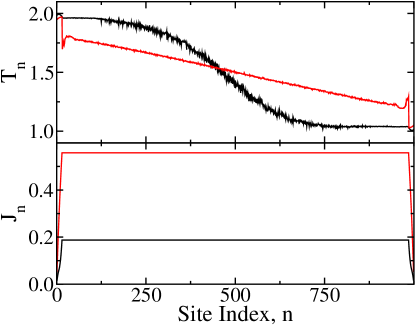
In the central section of the chain ($N_{b}<n<N-N_{b}$), which is not directly coupled to the bath, the NESS heat current has to be independent of $n$ due to continuity, i.e. $J=J_{n}$. In our proceeding numerics, the bath temperatures are fixed footnote1 at $T_{L}=2,\;T_{R}=1$. Additionally, all thermal calculations are averaged over $10^{2}$ realizations of disorder. An example of the local profiles is displayed in Fig.1 – in particular, the flat profile seen in $J_{n}$ confirms that continuity is fulfilled.

III Localization Properties

We consider the isolated case ($\lambda=0$). Substituting $q_{n}^{\nu}(t)=A_{n,\nu}\exp\left(i\omega_{\nu}t\right)$ results in an eigenvalue problem $-\omega_{\nu}^{2}{\vec{A}}_{\nu}=\mathbf{K}{\vec{A}}_{\nu}$. Again, note that the choice of the random distributions in the banded random matrix $\mathbf{K}$ ensures positive definite eigenvalues, $\omega_{\nu}^{2}\geq 0$. The extent of the modes is often characterized by their participation number (PN)

$$P_{2}=\frac{\left(\sum_{n}|A_{n,\nu}|^{2}\right)^{2}}{\sum_{n}|A_{n,\nu}|^{4}}.$$ (8)

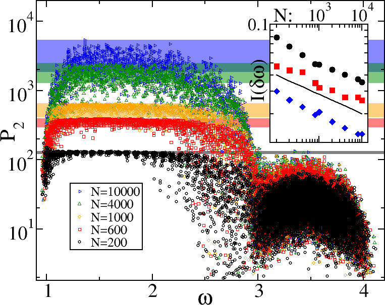
In Fig.2, the PN’s are plotted versus the eigenfrequencies for different finite lattice sizes and a fixed bandwidth of $b=5$. All states are localized ($P_{2}<N$), yet two windows are observed: a window of highly localized states for higher frequencies and a window of states with larger PN for lower frequencies.

Figure 2: (Color online) Participation number (PN) versus frequency for $b=5$. Various finite system sizes are delineated by colors. Colored stripes indicate the groups of the most extended modes, for which $P_{2}\geq 0.6P_{2}^{\rm max}$. A normalized count of selected states yield a scaling $I\sim N^{-\gamma}$ for the integrated density of states (IDoS), as shown in the inset, for three representative bandwidths: $b=5$ (black $\bullet$), $b=10$ (red $\blacksquare$), and $b=12$ (blue $\blacklozenge$). The best fit indicates $\gamma\approx 0.1\pm 0.05$ (black solid line).

We define the spectral window $\delta\omega=\omega_{\rm max}-\omega_{\rm min}$, whereby the modes with the larger PN are supported by the condition $P_{2}(\omega)\geq 0.6P_{2}^{\rm max}$. This allows us to find a scaling behavior for the integrated density of states (IDoS) of these modes

$$I\left(\delta\omega\right)=\int_{\omega_{\text{min}}}^{\omega_{\text{max}}}\rho(\omega)d\omega\sim N^{-\gamma},$$ (9)

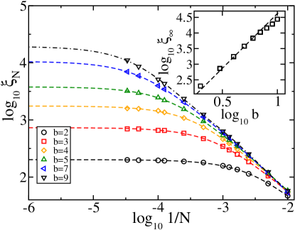
Our results for various values of bandwidth $b$ are shown in the inset of Fig.2. The solid line indicates the best fit with $\gamma=0.1\pm 0.05$. The averaged (over the spectral window $\delta\omega$ and over disorder realizations) PN is $\xi_{N}=\langle P_{2}\rangle_{\delta\omega}$, reported in Fig.3 for various $b$-values versus $1/N$. Typically, more than $10^{4}$ eigenvectors were used for the averaging. We find that $\xi_{N\rightarrow\infty}(b)$ shows a convergence towards a finite value $\xi_{\infty}(b)$. For moderate $b$-values this asymptotic PN is reached, while for larger bandwidths it can be extrapolated from the quotient of two fifth order polynomials fitted to the data (dashed/dotted -dashed lines in the figure). Inspired by previous studies on the localization properties of BRM’s CMI90 ; KPIR96 ; BKS10 , we speculate that the asymptotic PN will scale as $\xi_{\infty}\sim b^{\eta}$. Our expectation is nicely confirmed by the numerical data, reported in the inset of Fig. 3. The best fit indicates that $\eta\approx 3.5$, and thus $\xi_{\infty}(b)\sim b^{3.5}$.

Figure 3: (Color online) Main: The disordered and spectral (over $\delta\omega$) averaged PN $\xi_{N}$ against $1/N$, for various $b$-values. Saturation of $\xi_{N}$ as $N\rightarrow\infty$ is observed for moderate bandwidths. For larger values of $b$ a fitting of the data to a rational function of fifth order polynomials (dashed/dot-dashed lines) allows to extract the limit $\xi_{\infty}$. Inset: Parametric dependence of $\xi_{\infty}$ on $b$. The dashed line is the power relation $b^{3.5}$.

IV Scaling Theory

Equipped with knowledge of the localization properties of the normal modes of our system in Eq.(3), we now turn to the study of the steady-state heat current of Eq.(7). This is formally expressed as $J=\int_{0}^{\infty}\rho(\omega)\tau(\omega)d\omega\approx\int_{\omega_{\rm min}}^{\omega_{\rm max}}\rho(\omega)\tau(\omega)d\omega,$ where $\rho(\omega)$ is the density of states and $\tau(\omega)$ is the frequency dependent transmittance. Since heat is transported significantly only by the modes with the larger PN, we confine the integration range within the spectral window $\delta\omega$. These modes have similar localization – and therefore transport – properties, as shown previously. Therefore, we approximate $\tau(\omega)$ by its average value over this window $\langle\tau\rangle_{\delta\omega}$. The remaining integral is then just the IDoS of Eq.(9). We can now use knowledge for the transmittance of harmonic chains to deduce a scaling relation for the rescaled heat current ${\tilde{J}}\equiv J/N^{-\gamma}\propto\langle\tau\rangle_{\delta\omega}$.

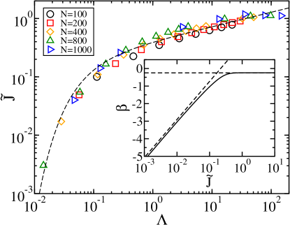
Specifically, the transport theory of disordered media predicts that the average transmittance $\langle\tau\rangle_{\delta\omega}$ of a disordered sample of length $N$ which is characterized by a localization length $\xi_{\infty}$ follows a one-parameter scaling $\langle\tau\rangle_{\delta\omega}=f_{T}(\Lambda)$, where the one parameter is $\Lambda\equiv\xi_{\infty}\ /N$. It is natural to then speculate that the same scaling relation will apply for the rescaled heat current ${\tilde{J}}$. In the main panel of Fig.4 we show our numerics of ${\tilde{J}}$ plotted against $\Lambda$, for a number of different bandwidths and system sizes ($b\in[2,35],N\in[10^{2},10^{3}]$). In this approach, we have used $\xi_{\infty}$ as a scaling parameter, which allows us to collapse all data associated with various $b$-values to one scaling curve. By visual inspection footnote2 , we find that the scaling parameter $\xi_{\infty}\sim b^{3.5\pm 0.2}$, which confirms the previous independent scaling analysis from the participation numbers (see Fig.3 and its discussion). The obvious data collapse confirms the conjecture that ${\tilde{J}}_{N}(\xi_{\infty})$ is a function of $\Lambda$ only i.e. ${\tilde{J}}_{N}(\xi_{\infty})=f_{\tilde{J}}(\Lambda)$.

Figure 4: (Color online) Main: Rescaled heat current ${\tilde{J}}$ vs. $\Lambda=\xi_{\infty}/N$ where $\xi_{\infty}\sim b^{3.5}$ as was found from Fig.3. The dashed line is a fit to the analytical curve of Eq.(10). Inset: The resulting $\beta$-function of Eq.(1). The dashed lines correspond to the asymptotic limits of $\beta=1.28+0.94\cdot\ln{\tilde{J}}$ for $N\rightarrow\infty$ and $\beta=-\nu$ for $N\rightarrow 0$.

Next we want to determine the analytical form of the scaling function $f_{\tilde{J}}(\Lambda)$. We have found that in the limit of the localized regime ($\Lambda\ll 1$) this dependence has the form ${\tilde{J}}\sim e^{-c_{0}/\Lambda}$, in agreement with previous theoretical results for pinned harmonic chains with only nearest neighbor coupling and mass disorder DL08 . In the other limit of $\Lambda\gg 1$, the heat transport is diffusive. Assuming validity of the Fourier law, we may expect a scaling of the type ${\tilde{J}}\sim 1/N^{1-\gamma}$ – however, recent investigations lepri_stochastic_2009 ; KCRDLS10 found an anomalous behavior of the heat current, which results in the scaling ${\tilde{J}}\sim 1/N^{\alpha-\gamma}$. We therefore speculate that in the diffusive domain of $\Lambda\gg 1$, the rescaled steady state heat current will follow the relation ${\tilde{J}}(\Lambda)\sim c_{1}\Lambda^{\nu}$. A possible interpolating law valid in all regimes (including the crossover region) is

$${\tilde{J}}(\Lambda)=(c_{2}+c_{1}\Lambda^{\nu})\exp(-c_{0}/\Lambda).$$ (10)

Comparison with numerical data in the two limits ($\Lambda\gg 1$, $\Lambda\ll 1$) yields $\nu\approx 0.25$, $c_{1}\approx 0.4$ and $c_{0}\approx 0.06$. Adjusting the last parameter $c_{2}$ to fit numerics in the intermediate region yields $c_{2}\approx 0.012$. The resulting analytical formula nicely fits the numerical results in all regions, and therefore provides a compact summary of our empirical data (see dashed line in Fig.4). We stress that the limiting value of $J(\Lambda\gg 1)\propto 1/N^{\gamma+\nu}$ leads to an anomalous heat exponent $\alpha\approx 0.35\pm 0.05$. It should be noted that this value is less than what has typically been seen in other - nonlinear and disordered - chain models, which show values from $\approx 0.4-0.7$ ivanchenko_disorder_2011 ; mai2007 ; D01 ; lepri_stochastic_2009 ; RD08 ; KCRDLS10 .

Eq.(10) can be rewritten in the form of Eq.(1). This is the main result of the present Letter, as it allows postulating the existence of a $\beta$-function for the ${\tilde{J}}_{N}$ of generic quasi-$1D$ disordered systems. The resulting $\beta$-function is plotted in the inset of Fig.4. Its asymptotes are seen to follow $\beta=1.28+0.94\cdot\ln{\tilde{J}}$ for $N\rightarrow\infty$, and $\beta=-\nu$ for $N\rightarrow 0$.

V Conclusions

We presented a one-parameter scaling theory for the steady-state heat current of quasi-one dimensional disordered harmonic systems with substrate pinnings described by a variant Banded Random Matrix ensemble. Via numerical analysis and theoretical considerations, we have established Eq.(1), which allows us to conclude that changing disorder strength (or coupling range) and system size in the way described by Eq.(10), would not change the renormalized (average) heat current. The one-parameter scaling theory presented here is a powerful approach in the quest of understanding thermal transport, and validity of the Fourier law, in disordered media. Of further interest will be to investigate higher moments of the NESS heat current and also to establish a scaling theory for the thermal profile, as a function of the scaling parameter $\Lambda$. Although the focus of this Letter was on harmonic quasi-1D disordered phononic transport, our approach can be used to study high-dimensional pinned harmonic systems, and to better understand the effects of phonon-phonon interactions BKS10 in thermal transport.