Retrieving Atmospheric Dust Opacity on Mars by Imaging Spectroscopy at Large Angles
Résumé
We propose a new method to retrieve the optical depth of Martian aerosols (AOD) from OMEGA and CRISM hyperspectral imagery at a reference wavelength of 1 m. Our method works even if the underlying surface is completely made of minerals, corresponding to a low contrast between surface and atmospheric dust, while being observed at a fixed geometry. Minimizing the effect of the surface reflectance properties on the AOD retrieval is the second principal asset of our method. The method is based on the parametrization of the radiative coupling between particles and gas determining, with local altimetry, acquisition geometry, and the meteorological situation, the absorption band depth of gaseous CO2. Because the last three factors can be predicted to some extent, we can define a new parameter that expresses specifically the strength of the gas-aerosols coupling while directly depending on the AOD. Combining estimations of and top of the atmosphere radiance values extracted from the observed spectra within the CO2 gas band at 2 m, we evaluate the AOD and the surface reflectance by radiative transfer inversion. One should note that practically can be estimated for a large variety of mineral or icy surfaces with the exception of CO2 ice when its 2 m solid band is not sufficiently saturated. Validation of the proposed method shows that it is reliable if two conditions are fulfilled: (i) the observation conditions provide large incidence or/and emergence angles (ii) the aerosol are vertically well mixed in the atmosphere. Experiments conducted on OMEGA nadir looking observations as well as CRISM multi-angular acquisitions with incidence angles higher than 65° in the first case and 33° in the second case produce very satisfactory results. Finally in a companion paper the method is applied to monitoring atmospheric dust spring activity at high southern latitudes on Mars using OMEGA.
keywords:
Mars; Atmosphere; Radiative Transfer; Aerosols; OMEGA; CRISMIntroduction
Visible and near infrared imaging spectroscopy is a key remote sensing technique to study and monitor the planet Mars. Although its atmosphere is much fainter than Earth’s, its composition dominated by CO2 gas implies numerous and strong absorption bands that often overlap with spectral features coming from the surface. Furthermore small mineral particles or H2O ice clouds often drift over Martian surfaces at various altitudes. These aerosols have also a strong, spatially and temporally varying influence on the morphology of the acquired spectra. As a consequence accurate analysis for the study of surface materials requires the modeling and the correction of the atmospheric spectral effects. The first step in this matter consists in retrieving the aerosol optical depth (AOD) over the scene.
Since 2004 the imaging spectrometer OMEGA aboard Mars Express performs nadir-looking and EPF (Emission Phase Function) observations in the VIS (visible) and the SWIR (short wave infrared) (920-5100 nm at 14 to 23 nm spectral resolution) for the study of the surface and the atmosphere of the red planet. See Clancy and Lee (1991) for the definition of the EPF mode. The spatial resolution of OMEGA typically varies between 300 and 2000 m/pixel due to its eccentric orbit. The authors in Vincendon et al. (2007) have developed a method to quantify the contribution of atmospheric dust in SWIR spectra obtained by OMEGA regardless of the Martian surface composition. Using multi-temporal observations at nadir with significant differences in solar incidence angles, they can infer the AOD and retrieve the surface reflectance spectra free of aerosol contribution. However, this method relies on the very restrictive assumption that the atmosphere opacity remains approximately constant during the time spanned by the employed acquisitions.
In Vincendon et al. (2008) the same authors map the AOD in the SWIR above the south seasonal cap of Mars from mid-spring to early summer. This mapping is based on the assumption that the reflectance in the 2.64 m saturated absorption band of the CO2 ice at the surface is mainly due to the light scattered by aerosols above most places of the seasonal cap. In this case, one geometry is sufficient for the AOD retrieval. Nonetheless, this method is restricted to the area of CO2 deposits that are not significantly contaminated by dust nor water ice.
The Compact Reconnaissance Imaging Spectrometer for Mars (CRISM) is a hyperspectral imager on the Mars Reconnaissance Orbiter (MRO) spacecraft. In targeted mode, a gimbaled Optical Sensor Unit (OSU) removes most along-track motion and scans a region of interest that is mapped at full spatial and spectral resolution (18 or 36 m/pixel, 362-3920 nm at 6.55 nm/channel). In the targeted mode, ten additional, spatially binned images (180 m/pixel) are taken over the same region before and after the main image at 10 emergence angles ranging from -70° to 70°. They provide the so-called Emission Phase Function (EPF) for the site of interest that is intended for atmospheric study and correction of atmospheric effects.
Regarding the atmospheric correction of CRISM data, McGuire and 14 co-authors (2009) adapted and improved the so-called volcano-scan technique (Langevin et al., 2006). This method removes the CO2 gas absorption bands of any spectrum of interest after division by a scaled reference spectrum (i.e. the ratio between the atmospheric transmission at the summit and the base of Olympus Mons evaluated on a Martian sol when the amounts of ice and dust aerosols were minimal). This simple technique works reasonably well for surfaces spectrally dominated by minerals, water ice, and sometimes CO2 ice but does not correct for aerosol effects .
In McGuire and 23 co-authors (2008), a DISORT-based model retrieved the dust and ice AOD, the surface pressure and temperature from previous experiment products as well as the acquisition geometry, and the measured I/F spectrum as inputs. Then, a surface Lambertian albedo spectrum is computed as the output. However this algorithm does not retrieve the AOD directly from the images nor does it take advantage of the EPF measurements of the CRISM targeted mode.
Brown and Wolff (2009) proposed a first attempt in that direction by using the DISORT algorithm to model the signal at one wavelength (i.e. 0.696 m). They iteratively adjust three parameters (surface albedo, dust and ice opacity) in order to achieve a close fit at five points spread across the EPF curve. Nevertheless the method is time consuming and the surface albedo is assumed to be Lambertian. It has been proved that this assumption bias the AOD and surface estimation (Lyapustin, 1999).
In this article, we propose an original method that overcomes the previous limitations to retrieve the optical depth of the Martian dust from OMEGA or CRISM data at the reference wavelength of one micron. The method is based on a parametrization of the radiative coupling between aerosol particles and gas that determines, based on the local altimetry and the meteorological situation, the absorption band depth of gaseous CO2. We consider the intensity of the absorption feature at 2 m as a proxy of the AOD, provided that the other influencing factors have been taken into account. Our method relies on radiative transfer calculations that assume lambertian properties for the surface even though, as demonstrated in this paper, the influence of the latter hypothesis is minimized by considering the effect of the aerosols on the gaseous absorption and not the total signal. When processing OMEGA observations, we are complementary to the method of Vincendon et al. (2008) since our approach processes pixels occupied by a wider variety of materials - pure mineral or water ice as well as CO2 and H2O deposits contaminated by a large amount of dust - while being observed at a fixed geometry. When processing CRISM observations we take full advantage of the top of the atmosphere spectral EPF measured by the instrument for the retrieval of the AOD.
This article is organized as follows. In section 1 we describe the post-processing and the formatting of the sequence of EPF calibrated image cubes accompanying the high resolution CRISM observation. In section 2, we give insights about Martian atmospheric properties and radiative transfer (RT) in the SWIR range. Furthermore we describe models that calculate the spectral radiance coming from Mars and reaching the sensor at the top of the atmosphere. In section 3 we expose the basic assumptions, RT parametrization, and properties on which relies the method for retrieving the AOD from the images. In addition we describe how we implement the method that is then validated on synthetic data. Finally, in section 4, we present and discuss results obtained for representative observations, one from OMEGA and the others from CRISM. Conclusions are eventually drawn in the last Section.
1 Post-processing and formatting of CRISM EPF observations
Due to the composite nature of CRISM EPF acquisitions, such data need some post-processing prior to AOD retrieval. First of all, CRISM data are transformed from apparent I/F units (i.e. the ratio of reflected radiance to incident intensity of sunlight) to reflectance units. A Lambertian surface is supposed and data are divided by the cosine of the solar incidence angle (Murchie and 49 co-authors, 2007).
CRISM data are corrected for artifacts caused by non-uniformities of the instrument, residuals of the radiometric correction or external sources. First, hyperspectral images are corrected for striping and spiking effects. Corrections for both distortions have been proposed by Parente (2008). Secondly, the CRISM spectrometer is affected by a common artifact to “push-broom" sensors, the so-called “spectral smile" effect. Smile effects refers to the artifacts originated by the non-uniformity of the instrument spectral response along the across-track dimension, i.e., the horizontal axis that corresponds to the data columns. The mitigation of smile effects is crucial since the spectral band corresponding to the absorption maximum of the CO2 gas at 2m is particularly affected by spectral smile. We remember that the proposed AOD retrieval method is based on this spectral feature. As a matter of fact, the estimation of the AOD might be biased if smile effects are not addressed. Ceamanos et al. developed a twofold method that corrects CRISM observations for smile by mimicking an optimal smile-free spectral response (Ceamanos and Doute, 2010). Nevertheless since uncertainties associated to the method itself might propagate to the AOD retrievals we conservatively restrict the use of each spatially binned image to the central columns that own the best spectral response the so-called “sweet spot” columns. This decimation of the data is not a problem because the EPF sequence provides plenty of points for each eleven geometries.
CRISM observations are spatially rearranged to evaluate the atmosphere optical depth of a given terrain position depending on geometry. First, the central image that owns the highest spatial resolution is binned by a factor of ten to match the spatial resolution of the EPF series. After that, all images are projected onto the same geographical space. At this point, CRISM observations showing a high overlap of the eleven acquisitions can be discriminated. In fact, a good overlap assures the existence of a high number of terrain units that have been sensed from many geometries. In a single hyperspectral data set that gathers all EPF images and the central scan (hereafter called CSP, Cube SpectroPhotometric), each super pixel conjugated to a given terrain unit gathers up to eleven spectra depending on the completeness of the overlap. More details can be found in (Ceamanos et al., 2013).
2 Mars atmospheric radiative transfer
In the present section we give insights about Martian atmospheric properties and radiative transfer (RT) in the SWIR range. Furthermore we describe models that calculate the spectral radiance coming from Mars and reaching the sensor at the top of the atmosphere.
We consider the Martian atmosphere as a vertically stratified medium with a plan parallel or spherical geometry. We divide the atmosphere into 30 layers spanning the 0-100 km height range. The lower boundary of the layer is at height above the surface. Each layer contains a mixture of gas and solid particles and is homogeneous in temperature [K], pressure [mbar] and gaseous composition [ppm].
2.1 Gas
A dozen atmospheric absorption bands due to gaseous CO2 and marginally to H2O are present in the SWIR. We calculate the transmission function of the atmosphere along the vertical, for each pixel of our spectral images, and as a function of wavelength.
LBLRTM
For that purpose, we employ a line-by-line radiative transfer model (LBLRTM) (Clough et al., 1995) fed by the vertical compositional and thermal profiles predicted by the European Mars Climate Database (EMCD) Forget et al. (2006) for the dates, locations, and altitudes of the observations. The LBLRTM code takes into account the vertical profile of temperature, pressure and gaseous composition and interrogates the spectroscopic database HITRAN (<<high-resolution transmission molecular absorption database>>, http://www.cfa.harvard.edu/hitran/) to compute for each homogeneous layer the monochromatic absorption coefficient [m] () of the gaseous mixture for the wavenumber . The absorption lines typical of each molecular specie are characterized by a <<Voight>> profile that describes at the same time the broadening by Doppler effect and by collision. The code LBLRTM from the Atmospheric and Environmental Research (AER) company also takes into account various spectroscopic coupling between species (some of them not being directly active in the optical sense like N or the inert gases). If [m] is the vertically integrated molecular density in terms of number in layer , the vertical monochromatic transmission follows the Beer-Lambert law:
Method k-correlated coefficients
In order to take into account the fine details of the gas lines, the final RT calculation, which will integrate the gaseous as well as particulate absorption and scattering, should be conducted in principle according to the maximum spectral resolution of the problem (). Since we must simulate tens, even hundreds, thousand spectra with numerically intensive codes, such a requirement cannot be satisfied practically. Each spectral channel of the sensors that we consider (see Introduction) presents a width 10 cm and thus contains hundreds of lines that cannot be considered individually. Consequently, only a statistical approach like the one proposed by Goody et al. (1989) offers a practical solution of the problem. Starting from the line spectra in the spectral interval (, being the lower bound of the current channel ), we build the discrete form of the frequency distribution for the absorption:
| (1) |
is a partition of the interval of values taken by the monochromatic absorption coefficient in , the number of spectral points having a value falling in the bin of lower bound and of width .
First, we choose an irregular partition that gives the same number of points for each bin . The objective is to estimate numerically the frequency (i.e. a probability) with bins all containing the same number of individuals (, a number large enough to guaranty a correct and homogeneous accuracy. Because there are much more lines of weak intensity than lines of strong intensity, the width is a strongly increasing function of . From the discrete form of the cumulative frequency distribution is derived such as: . The inverse function , which is generally defined in the literature as a <<k distribution>> and is established in the interval , is the highest absorption value reached by the lower fraction of the population of lines ordered according to their intensity. In practice, the previous function is calculated for any value of by spline interpolation of the experimental curve passing through the points .
Second, we split the line population in () sub-sets each representing a fraction , and of the total. A Gaussian quadrature of order N=2 for example allows an optimal sampling of the weak and strong absorption values. Then, the function allows to build the corresponding partition but in the space of absorption values . We calculate the mean value of the monochromatic absorption coefficient in each bin thanks to the values returned by LBLRTM AER.
Finally, as in Lacis and Oinas (1991), we assume that the mean transmission value for the instrument channel through the layer is:
| (2) |
Furthermore, we introduce a mean optical depth linked to the sub-sets , each representing a fraction of the population of lines sorted by increasing intensity : . Then with the set of coefficients associated to the Gaussian partition .
Spectral transmittivity
If we now consider the whole stack of atmospheric layers, we must make an additional hypothesis in order to calculate an approximation of the total vertical transmission. It is based on the fact that the atmospheric composition does not change significantly over the heights spanned by the region that contributes predominantly to the transmission. Thus, the form of the distribution is very similar from one layer to the other even though the absolute level -which depends on the pressure level for example- varies. Indeed, if an intense absorption line is centered at wavenumber for layer then the line originating from the same transition has a high probability of falling nearly at the same position for the layer even though its width and intensity are different. In other words, the probability that a strong absorption level in the layer at wave number is associated to a weak level in the layer is very low. Statistically such a situation translates to the following rule concerning the probability that the absorption level for the wavenumber belongs to the sub-set in the layer and to the sub-group in the layer : (Kronecker symbol). The transmission through both layers that should be generally written:
| (3) |
can then be approximated by :
| (4) |
since we use the same quadratures for both layers. This formula can be generalized to the whole stack of layers and the vertical transmission through the atmospheric gases in a multilayered medium is given by:
| (5) |
Because the complete calculation is very time consuming, it is only performed for a limited () number of reference points representative of “regions” sliced according to regular bins in latitude , longitude and altitude . Three transmission spectra are generated for the maximum, mean and minimum altitude of a given region. Then the transmission spectrum of all the pixels belonging to the region is interpolated from the triplet depending on their individual altitude to give
2.2 Aerosols
Optical properties of Martian mineral aerosols are still largely undocumented even though recent studies have improved our understanding (Korablev et al., 2005). We favor the single scattering albedo, optical depth spectral shape and phase function retrieved in the near-infrared by Vincendon et al. (2008) and Wolff et al. (2009). In the first case,a Henyey-Greensten phase function with one parameter is used. This is a coarse parametrization but it is relevant for the phase angle range spanned by the data set of nadir OMEGA observations that we consider. In the second case, because it has been proved that the Henyey-Greenstein function is somewhat inaccurate to recreate the effect of aerosols for the CRISM angular ranges, the radiative properties are described with more details. A single scattering albedo, optical depth spectral shape, and phase function based on cylindrical particles are considered. The composition of aerosols has been shown to be remarkably homogeneous, e.g. between Rover landing sites. Changes of radiative properties (Vincendon et al., 2009) mainly result from differences in the mean of the aerosols size distribution (Wolff et al., 2003) because the latter results from a balance between sedimentation and lifting mechanisms, which in turn depend on turbulence, density, etc. Additionally the degree of hydration for the mineral particles might change with latitude and season . Fortunately, for the typical hydration values reached on Mars, the spectral effects are only noticeable between 2.7 and 3.5 m (Pommerol et al., 2009), a range that we thus ignore. Water ice crystals may also be frequently present but are not considered in this paper because they may influence the CO2 gas 2m absorption feature in a specific manner. Because the atmosphere is usually well mixed, we take a vertical distribution of optical depth at a reference wavelength ( : 1 m) that is exponentially decreasing with height such that:
is the column integrated opacity of the aerosols at the reference channel , is the scale height of the distribution, the height of layer lower interface and km. The scale height and the optical depth remain the only free parameters concerning the atmosphere.
2.3 Gas-aerosols coupling
In general, photons undergo absorption and multiple scattering events when interacting both with gas and aerosols. One should note that we neglect Rayleigh scattering due to atmospheric molecules because, according to the formula of Bodhaine et al. (1999), that will lead for a mean ground pressure of 6 mbar to an optical depth of - far lower than the contribution we can expect for the aerosols in any case. The value of the monochromatic aerosol optical depth (at ) does not vary significantly within a channel whereas the counterpart for the gas can vary by several orders of magnitude. As a consequence calculating at channel the transfer of radiation in the atmosphere requires to couple gas and aerosols properties at each atmospheric level and for each sub-set of the gas line population. As indicated in Table 1, the coupling procedure leads to sets of optical depth, single scattering albedo and phase function that characterize the layers. These properties, as well as the acquisition geometry (), are introduced one by one in a RT engine (e.g. DISORT, Stamnes et al. (1988)) in order to calculate for each level the partial radiance field corresponding to each sub-set lines+aerosols. The surface is characterized by its bidirectional reflectance distribution function (BRDF). The total radiance field is the mean value of the partial fields weighted by the fractions :
| (6) |
3 Method for retrieving the optical depth
The proposed method is based on a parametrization of the radiative coupling between aerosol particles and gas that determines, with local altimetry and the meteorological situation, the absorption band depth of gaseous CO2. The coupling depends on (i) the acquisition geometry (ii) the type, abundance and vertical distribution of particles (iii) the bidirectional reflectance factor of the surface (BRF). For each spectrum of an image, we compare the depth of the 2 m absorption band of gaseous CO2 that we estimate on the one hand from the observed spectrum and on the other hand from a calculated transmission spectrum through the atmospheric gases alone. This leads to a relevant new parameter that directly depends on . Combining the latter with the radiance factor within the 2 m band, we evaluate by RT inversion the AOD and the reflectance factor of the surface.
3.1 Parametrization of the spectral signal
Our method is based on two main assumptions:
1. First we assume that the surface reflects the solar and atmospheric radiation isotropically and, consequently, that the ground-atmosphere interface is characterized by a single scalar quantity (the normal albedo ) that depends on wavelength.
2. Second we parametrize the radiative coupling between aerosols and gas by assuming that the latter contribute to the signal as a simple multiplicative filter. In this way, the top of the atmosphere (TOA) radiance is written such that
| (7) |
the effect of the acquisition geometry, the aerosols, and the surface
Lambertian albedo being taken into account by scaling
the aerosol free vertical transmission
-calculated according to 2.1- by an exponent .
is the calculated
TOA radiance but without considering the atmospheric gases in the
radiative transfer. Factor can be further decomposed
into two terms:
| (8) |
with the airmass . Factor is purely geometric and allows a quick and simplified calculation of the free gaseous transmission along the acquisition pathlength (incident-emergent) using the vertical free transmission :
| (9) |
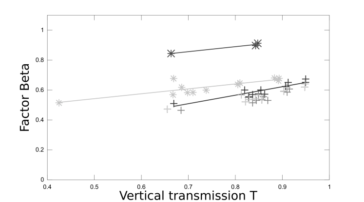
the approximate formula being . In order to retrieve the values of the factors to , we fit the experimental cloud of points obtained by plotting as a function of the airmass for a set of representative atmospheric vertical profiles. For that purpose the quantities and are respectively the slant and vertical versions of the free transmission through the gas given by the LBLRTM code. Note that the dispersion around the mean curve is very limited. . Factor accounts for the difference of spectral resolution and radiometric calibration between OMEGA and CRISM and its retrieval is explained at the end of section 3.5. All p-factor values are given in Table 2.
Factor on the other hand expresses the aerosol effect on gaseous absorption and depends on the considered channel . In practice this spectral dependability can be easily managed. Indeed, numerical experiments and the analysis of real data (see following sections) show that this exponent depends principally on the gaseous absorption intensity . If (i) can be estimated experimentally () for one or for several geometries for each pixel (super-pixel) of an OMEGA (CRISM) observation and (ii) if one assumes a value for ( is the spectral band number at 2m) then can be derived. Indeed, function is invertible provided that the scale height of the aerosols is known. In this matter, several studies such as Vincendon et al. (2008) suggest that km is a good guess, but in section 4 we prove that km may be more appropriate as it leads to better results.
3.2 Numerical aspects LUT
Our optical depth retrieval system uses a multi-dimensional look-up table (LUT) of values arranged according to discrete combinations of acquisition geometries and of physical parameters , see Table 3. For each combination, the value of is calculated on the basis of three TOA spectra. is a reference free vertical transmission corresponding to a given time and location on the surface of Mars. It has been chosen in order to cover a range of absorption values (all spectral bands considered) typical of the southern hemisphere in spring. The spectra and in units of radiance are generated successively by the code DISORT with and without considering the gaseous absorption in the atmosphere. A series of k-correlated coefficients intervenes in the calculation of and . Finally the LUT is built according to the formula:
| (10) |
with . The channels () encompass the 2 m CO2 gas absorption band such as . For DISORT calculations, we consider the atmosphere as a plan parallel vertically stratified medium which is a sufficient approximation to calculate the TOA radiance whenever incidence and emergence directions are 10o above the horizon. Several experimental scatter-plots - built using the reference and also other sets of k-correlated coefficients show that there exists a linear relationship between the two quantities with an excellent correlation factor ( see figure 1) :
| (11) |
We notice that the coefficients of the regression depend weakly on the parameters .
3.3 Estimation of the coupling factor gas-aerosols
Because the intensity of the CO2 gas 2m absorption feature is diversely accessible from the spectra depending on the nature of the surface materials present in the pixel, we need to consider different strategies for estimating the factor .
Mineral surfaces: method 1
The factor can be readily estimated for every OMEGA or CRISM spectrum that does not show any features, such as the H2O or CO2 ice signature, superimposed on the 2 m CO2 gas absorption band. In this way, this absorption band is completely due to the atmosphere. A similar formula to the one used in the volcano scan technique (McGuire and 14 co-authors, 2009) is used replacing the Olympus reference transmission spectrum by such that
| (12) |
with the index of a channel falling at the shortwave extremity of the 2 m band wing. The scatter-plot -, built for each pixel of a real OMEGA observation confirms the existence of a linear relationship between the two quantities with a generally moderate dispersion (see Figure 1). The regression coefficients are then calculated and will allow us to estimate exponent in the same absorption range than the reference :
| (13) |
Note that we use the series of channels for the estimation of allowing us to be less sensitive to noise and channel aging than using the single channel . In order to perform the inversion process, we take as an initial value for the lambertian albedo of the surface .
Water ice surfaces: method 2
A specific procedure is necessary for any spectrum marked by the signature of water ice with the possible presence of dust but without spectral contamination by CO2 ice. A numerical optimization is performed regarding a cost function that depends on and that expresses the quality of the gaseous absorption correction on the spectra. The quality criteria we choose is the band shape of solid H2O at 2 m that must show a unique local minimum and a simple curvature. Mathematically this criteria is equivalent to the second derivative of the spectrum that must be close to zero for channels covering the H2O band and slightly beyond. After all the cost function is written:
| (14) |
Searching for the global minimum of this function leads to the estimation of the exponent : . The normalization of up to the reference level of absorption uses the regression line:
Once again, in order to realize the inversion we take as initial value for the lambertian albedo .
Carbon dioxide ice (CO2)
Currently there is no simple strategy to estimate in a pixelwise manner the coefficient from spectra presenting the signature of solid CO2 because the latter cannot be distinguished from its gaseous counterpart at 2m. For this kind of surface, our method to estimate is ineffective.
If, on the one hand, CO2 ice proves to be sufficiently pure with grain sizes more than 100 m in diameter (this conditions is always respected in practice for the seasonal deposits) then the method proposed by (Vincendon et al., 2008) is the only solution. It is based on the assumption that the reflectance level at 2.63 m (channel ) is nearly equal to zero because of the absorption saturation of the ice. Consequently, in this case, the reflectance factor represents the path radiance of the atmosphere (mostly due to the aerosols at channel ) and is a bijective, easily invertible function of . In section 3.5 we will see how exponent can be calculated from , computed using (Vincendon et al., 2008), and for correcting the gaseous absorption on the spectra (section 3.5).
If, on the other hand, CO2 ice proves to be substantially contaminated by dust or water ice, then the only conceivable way to estimate could be a statistical procedure as it is proposed in Luo et al. (2010).
Sulfates present a broad band similar to water ice around 2 m and are occasionally spectrally dominant in OMEGA or CRISM observations. A future requirement is finding a way to deconvolve the CO2 gaseous features from the sulfates 1.94 strong absorption in order to evaluate .
Hereafter, we simplify the writing of the parameters by removing subscript from the notations. The quantities and are as if they were wavelength independent because they are normalized up to the reference level of absorption.
3.4 Sensitivity and feasibility study.
Synthetic data
We now examine the sensitivity of function regarding its different parameters . This study is summarized as follows. The exponent decreases with the airmass especially as the aerosol opacity is on the rise. This is the direct consequence of an intensifying coupling effect between gas and aerosols, the latter reducing the effective pathlength of the photons in the atmosphere by scattering and thus the probability to be absorbed by CO2 gas. The exponent evolution reflects such a decrease of relative absorption band intensity. The coupling is higher when the sensor looks in the solar direction than when its looks in the opposite half space . The higher the scale height characterizing the vertical distribution of the aerosols, the more aerosols influence atmospheric absorption especially since their opacity is high. The surface reflectance factor also controls the absorption by CO2 gas because of occurrence of multiple scattering between the two media. A bright surface promotes a higher number of roundtrips for the photons which then have a higher probability to be absorbed: exponent increases with Lambertian albedo . Finally, because the sensitivity of with () decreases with the airmass, we can expect significant estimation errors for below a certain threshold. Indeed the ground pressure provided by the Martian climate database (Forget et al., 2006) is only indicative of the real pressure at the moment of the observation. We must stress that the ground pressure determines then and, for this reason, an uncertainty will propagate as an uncertainty on the coupling factor, then as an uncertainty on the optical depth . We quantify this effect in the validation section 3.6.
The experimental behavior of , evaluated above mineral surfaces based on real data with respect to airmass and , is also full of information. We distinguish two situations according to whether we work with OMEGA or CRISM observations.
OMEGA data
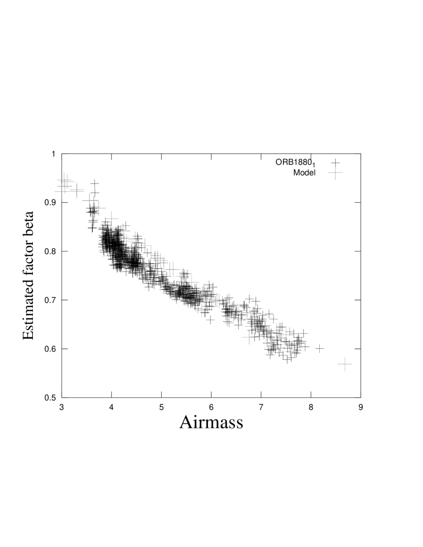
In the OMEGA case, we consider large populations of pixels extracted from several hyperspectral images. The principal variability of the aerosol opacity across the scene comes from altitude changes -sometimes several kilometers in elevation- that modify the local atmospheric height and thus the column integrated density of the aerosols. The horizontal heterogeneity of the particle density at constant altitude generally implies a more moderate variability. Hence, by selecting pixels belonging to slices spanning no more than a couple hundred meters in elevation but observed under various geometries, we can draw a scatter-plots () such as that presented in Fig. 2. Set apart a noticeable internal dispersion linked to factors such as those previously mentioned or spatial variations of Lambertian surface albedo, the points corresponding to the OMEGA observation 1880_1 are organized according to monotonously decreasing curves of over a wide range of increasing values. The curves faithfully follow the theoretical scatter plot that can be built thanks to the numerical reference LUT for 11 km and . The best fit gives an estimation of the mean optical depth 0.8.
CRISM data
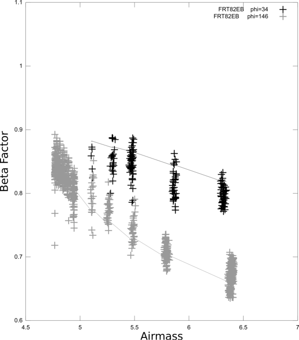
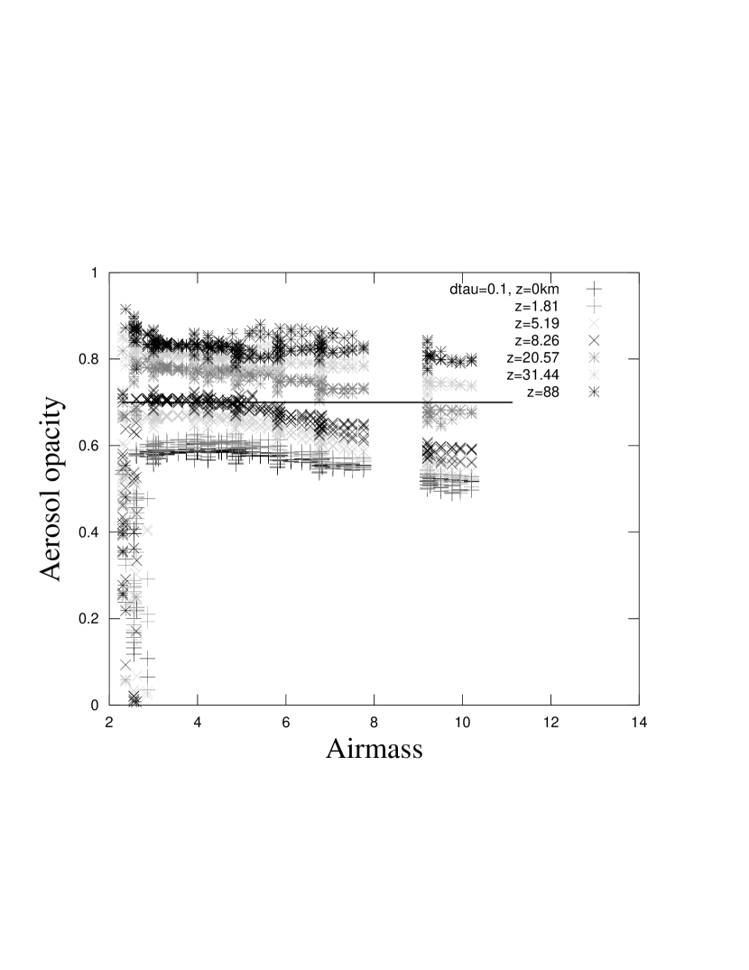
The sensitivity study is conducted on CRISM EPF sequence FRT82EB. This observation corresponds to an ice-free cratered area of the south pole of Mars (=-83∘). The image geometry corresponds to the conditions of the high latitudes with =74.5∘. Due to the sun-synchronous orbit of CRISM, there are two modes in azimuthal angle, 34∘ and 146∘. Regarding the topography, FRT82EB presents mild slopes and a constant altitude. The initial albedo of the surface can be approximated by the average value of the spectral band at 1 micron. In this case, the of FRT82EB is equal to 0.3.
Data are processed by the data pipeline described in Section 1, except the filtering of the columns affected by the “spectral smile” effect. Thanks to the good overlap of the high-resolution image and of the EPF, we can define up to 850 super pixels that are represented by more than 6 geometries.
The factor can be readily estimated for every CRISM spectrum that does not show CO2 ice signature superimposed on the 2 m CO2 gas absorption band. Once a series of spectra corresponding to a super pixel is treated, we obtain as a function of up to eleven geometries. Figure 3 summarizes the results for the image FRT82EB by plotting as the function of the airmass distinctively for the two azimuths explored by the observation (black and grey crosses).
One can see how the azimuthal angle has an impact on the gas-aerosol coupling due to aerosol phase function strong anisotropy (Wolff et al., 2009). In addition, the model curves of that provide the best matching with the experimental results are shown by plain lines. In fact, the best match corresponds to a value of around 0.5, respectively 8 km for . Curves for other targeted observations are shown in Fig. 10.
3.5 Algorithms for the simultaneous retrieval of surface albedo and aerosol opacity:
We now describe the practical implementation of the method that allows the computation of surface albedo and aerosol opacity maps from a given observation. The implementation comes in two flavors depending on the origin of the data.
OMEGA
The processing of a nadir OMEGA image is conducted on a pixelwise basis after segmenting the image according to an automatic detection of the surface components Schmidt et al. (2007). For the pixels that do not present the signatures of solid CO2 the following iterative algorithm is carried out:
Input: a spectrum of rank in the flattened
image, the corresponding vertical transmission calculated
as explained in section 2.1, the acquisition geometry
and a global estimation of the
scale height
-
1.
estimating the exponent
-
(a)
using method 1 (section 3.3) for a mineral
surface
-
(b)
using method 2 for a water ice surface without CO2 ice contamination
-
2.
initialization , Lambertian albedo
-
3.
DO
-
4.
building a 1D curve as a function
of by quadrilinear interpolation of the LUT described in
section 3.3 for a given set ,
and .
-
5.
linear interpolation of the previous curve at
to calculate
-
6.
building a 1D curve as a function
of by quadrilinear interpolation of the LUT for
a given set of and
-
7.
linear interpolation of the previous curve at
in order to calculate
-
8.
-
9.
UNTIL
The algorithm usually converges after a dozen iterations and leads to a complete solution once is calculated from and based on a dedicated LUT. If the initial estimation or, to a lesser extent, the estimation of is poor then the convergence is not reached and there is no solution.
For the pixels presenting a signature of solid CO2 pure enough (according to the criteria established by Vincendon et al. (2008)) we have seen in section 3.3 that it is possible to obtain by their independent method. The problem is then laid down differently: we must calculate the exponent from and that will be used for correcting the gaseous absorption on the spectra. The algorithm is also iterative in this case :
Input : a spectrum of rank in the flattened
image, the corresponding vertical transmission extracted
from the ATM cube at the same rank, the acquisition geometry
and a global estimation of the scale height
-
1.
estimation of using the method by Vincendon et al. (2008)
-
2.
initialization , Lambertian albedo
-
3.
DO
-
4.
building a 1D curve as a function of
by quadrilinear interpolation of the LUT described in section 3.3
for a given set ,
and .
-
5.
linear interpolation of the previous curve at
to calculate
-
6.
calculation of
-
7.
building a 1D curve as a function
by quadrilinear interpolation of the LUT for a
given set and
-
8.
linear interpolation of the previous curve at in order
to calculate
-
9.
-
10.
UNTIL
CRISM
The processing is applied to the single hyperspectral data set that gathers the central scan and the EPF images, i.e. the CSP cube. We choose an area of the image that offers the best compromise between its size and its spectral homogeneity. In addition, this area should not present the signatures of solid CO2. All the super-pixels that fall in the area are blended into one vector of parameters that needs to be explained as a whole by the model provided the solution for parameters and is found. The following iterative algorithm is carried out.
Input : the collection of valid spectra , the
corresponding vertical transmissions extracted from
the ATM cube at the same coordinates, the acquisition geometries
and a global estimation of the scale height
-
1.
for each valid pixel , estimating the exponent
-
(a)
using method 1 (section 3.3) for a mineral
surface
-
(b)
using method 2 for a water ice surface without CO2 ice contamination
-
2.
initialization , mean Lambertian albedo for the selected area
-
3.
DO
-
4.
building a matrix of values, each element
corresponding to the coupling factor that is predicted
by the model for the spectrum of index assuming that the atmospheric
opacity is, a sampling
of the range of possible variation for this parameter. The value
is calculated by quadrilinear interpolation of the LUT described in
section 3.3 for a given set ,
,
, and .
-
5.
finding the global minimum of the objective function
to
estimate
-
6.
for each valid pixel , building a 1D curve
as a function of by quadrilinear interpolation
of the LUT for a given set of
and . Linear
interpolation of the previous curve at
in order to calculate
-
7.
calculation of the mean Lambertian albedo
for the selected area
-
8.
-
9.
UNTIL
Note that the value of factor appearing in Table 2 is adjusted for the OMEGA (respectively CRISM) dataset by maximizing the overall convergence rate achieved by algorithms 3.5a (respectively 3.5c) for a selection of observations. Note that this optimization problem is satisfactorily convex and thus its solution satisfactorily constrained, since the convergence of the iterative inversion is very sensitive to the value of .
3.6 Validation
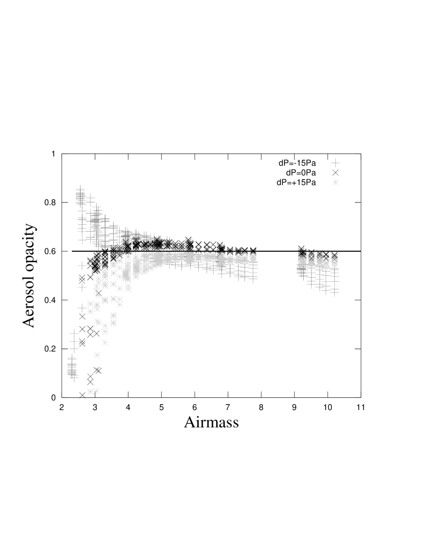
The validation is realized by inverting synthetic data, that is to say, realistic TOA spectra calculated with DISORT (section 2.3) to which we add zero-mean Gaussian noise simulated using a meaningful covariance matrix, i.e. calculated from an estimation of OMEGA noise. In the reference simulation, we set the properties of the surface (minerals) and of the atmosphere , km, and initial pressure . In a second simulation, for the calculation of the spectrum , we apply a pressure deviation of Pa typical of the Martian meteorological variability (barocline activity, (Forget et al., 1999)) but the factor is estimated with a transmission spectrum calculated according to the initial pressure. In a third simulation, we perturb the initial distribution profile of the aerosols (exponential) by increasing the opacity of one given layer in succession by an additional amount . Thus, the total AOD becomes 0.7 with the perturbed profile and there are as many runs as the layer number. In each run, the geometry varies according to the values given in Table 3. In agreement with the sensitivity study (section 3.4), Figure 4 shows that our method estimates with an accuracy comparable to the usual methods in the reference case provided that the airmass exceeds 3. Since we do not have access to the real ground pressure but to a value predicted by a MGCM, we expose ourselves to potentially important errors if but lower than 10% beyond (). Figure 5 illustrates the fact that a perturbation of opacity does not have the same impact on factor and thus on the estimation according to its height above the ground. A low lying aerosol layer is not detectable by our method because it does not have much influence on the mean pathlength of the photons into the gas. By contrast, a detached layer high in the atmosphere superimposed on the standard profile has a strong influence on the coupling. Thus, such a layer could skew our estimation because the latter does not take into account such a local perturbation. In conclusion, we state that our method is reliable if two conditions are full filled: (i) the observation conditions provide an airmass that is large enough, i.e. (ii) the aerosol particles are well vertically mixed caused by a vigorous convection.
4 Results
4.1 OMEGA
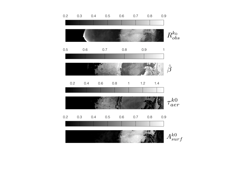
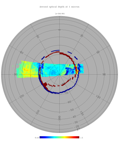
Figure 6 shows in a synthetic way all the products obtained by the chain of operations described above for the observation OMEGA ORB1880_1 that is representative of many. The chosen image covers a large geographical area of Mars at high and medium southern latitudes in spring. The bright extended part appearing in the maps and represents the seasonal deposits of frozen CO2 as well as the permanent cap that is, at that time, buried by the latter. The black coded area indicate the surfaces (among then a significant fraction of the “cryptic” region - where CO2 very much contaminated by dust exists - for which no method for estimating is currently available or indicate the pixels for which the iterative inversion has not worked (for example near the limb).
First cross validation of the two methods used in order to produce the map - ours and and the one by Vincendon et al. (2008)- can be performed as follow. We plot along-track profiles of optical depth through the maps and we examine to which extent the segments corresponding to the mineral surfaces (in black) and those corresponding to the frozen surfaces (in grey) are well connected in figure 7. The right-side red segment with high dispersion corresponds to the “cryptic” region. The quality of the connection seems quite good for ORB1880_1 and for other observations that we treated.
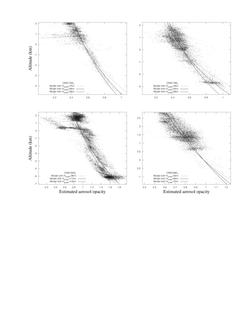
Second the problem of evaluating the dust scale height, which is an input of our retrieval algorithms, is investigated more thoroughly. Our region of interest is the southern high latitudes in spring for which dust activity is monitored in the companion paper. In this case there are two possibilities for constraining the dust scale height provided that it can be considered spatially constant for one given observation. First its value (along with factor ) can be adjusted by maximizing the overall convergence rate achieved by algorithm 3.5a when analyzing each image of a selection of OMEGA observations. In all cases =11 km turns out to be the optimal value. Note that this optimization problem is satisfactorily convex, and thus its solution satisfactorily constrained, since the convergence of the iterative inversion is very sensitive to the value of (, ). It is important to keep in mind that the previous scale height expresses the rate of optical depth change with height. Second large scale geographical variations of can be interpreted as due, at first order, to changes of the atmospheric column linked with changes of pixel altitude. Indeed if we assume that the intrinsic optical properties (such as the extinction cross-section ) and the scale height of dust particles are both geographically and vertically constant and that their density number normalized to altitude 0 is also geographically constant, then . We are restricted to OMEGA observations that cover an area with a range of altitudes large enough so that the experimental cloud of points obtained by plotting as a function of the pixel altitude can be satisfactorily fitted by the model. Figure 8 shows the result for four global observations. The data can be satisfactorily explained with values of varying from 6 to 11 kilometers, most often in the lower end of this interval, in agreement with Vincendon and Langevin (2010). We note that the “spatially” derived scale height does not correspond to the “radiatively” derived scale height () with the exception of observation ORB1849_1. If we trust the method a possible way to explain this discrepancy is to suppose that must show a overall systematic trend of decrease with altitude. In a sense this parameter expresses the intensity of dust loading in the atmosphere regardless of the length of the atmospheric column. We hypothesize that the systematic trend is linked with the decrease capability of the atmosphere to lift dust with the decrease of atmospheric density while the dispersion around the main trend is linked with the meteorological activity. If we assume also an exponential altitude profile with a scale height of for , the effective “spatially” derived scale height for is 6km for =11 km, consistent with what we found. Referring to Figure 8, it is interesting to note that the observation with the highest spatially derived scale height corresponds to a peak of dust activity around ° also observed by Pancam during MY27 (Lemmon and Athena Science Team, 2006). This global dust event erases the overall systematic trend of decrease with altitude.
Because it is impossible to constrain for each OMEGA observation we choose to take a fixed value =11 km. We have determined that possible excursions of by 3 kilometers from the reference value could lead to relative errors up to 50%.
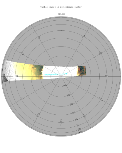
Finally an enlightening comparison is put forward between the AOD retrieved from our analysis of the near infrared 1880_1 image and an RGB composition made by extracting the TOA martian reflectivity measured by OMEGA at three wavelengths (0.7070, 0.5508, and 0.4760 m) from the corresponding visible image (Figure.9). The composition is stretched so as to make visible the dust clouds as yellowish hues against mineral surfaces while the seasonal deposits appear completed saturated. Excellent qualitative agreement can be noted between the two products down to the details. In the companion paper other successful examples are provided.
4.2 CRISM
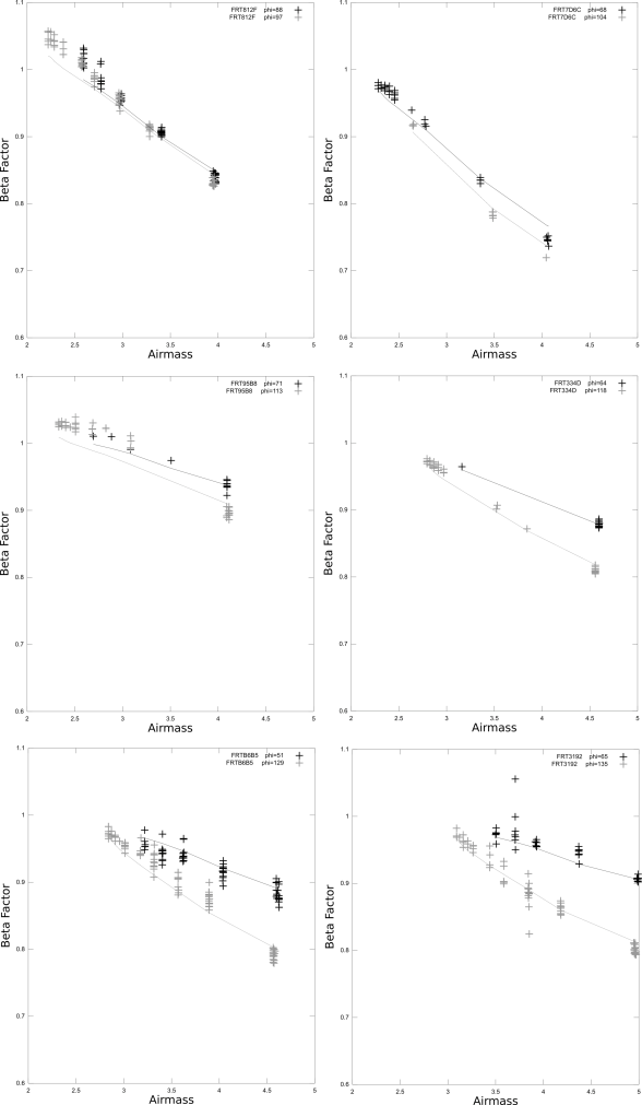
In the CRISM case, six observations of the landing site of the Mars Exploration Rover “Spirit” (i.e. West of Columbia Hills), acquired with varied geometry and atmospheric conditions (see Table 4), have been chosen to test our method (hereafter identified as the “ method”). For that purpose, these scenes are of special interest since the AOD values were also retrieved from the same data by Wolff et. al. (personal communication) and from PanCam synchronous measurements at the ground looking towards zenith (Johnson et al., 2006). The previous procedures are identified as the “W method” and the “P method” respectively. Special attention is paid by focusing on areas of the observations with altitude variations not exceeding one hundred meters and with negligible slope at the scale of the pixel size and above. Following the procedure described in section 1, the eleven CRISM images of each FRT observation are combined and binned at about 300 meters per pixel. Then, the algorithm adapted to CRISM for the simultaneous retrieval of surface albedo and aerosol opacity is applied on the CSP cube (section 1). The operation leads to the results tabulated in Table 4 along with those obtained by the “W” and “P” methods. In addition Figure 10 illustrates to which extent our best model matches the experimental versus airmass curves for each observation. Similarly to the OMEGA case, airmass represents a threshold above which the fit becomes very satisfactory with the exception of the observation FRT95B8. One should also note that the larger the difference between the two azimuthal modes is, the more constrained the best solution likely becomes because the two branches of the versus airmass curves are increasingly separated.
Once the content of aerosols is known, CRISM TOA radiances can be corrected in order to retrieve surface BRF. The correction of remotely sensed images for atmospheric effects is however not straightforward due to the anisotropic scattering properties of the atmospheric aerosols and the materials at the surface. Traditional inversion algorithms are based on reductionist hypothesis that assumes that the surface is lambertian (McGuire and 23 co-authors, 2008). Although this assumption largely simplifies the inverse problem, it critically corrupts the angular shape of the retrieved BRF since solid surfaces are hardly isotropic (Lyapustin, 1999). Recently, we have proposed an original inversion method to overcome these limitations when treating CRISM multi-angle observations Ceamanos et al. (2013). This inversion algorithm is based on a TOA radiance model that depends on the Green’s function of the atmosphere and a semi-analytical expression of the surface BRF. In this way, robust and fast inversions of the model on CRISM TOA radiance curves are performed accounting for the anisotropy of the aerosols and the surface. The root mean square error achieved by the model when reproducing the CRISM TOA reflectance factor curves is indicated in Table 4 for each observation and for each AOD input. A NaN value indicates that the inversion was not successful, i.e. no valid surface BRF could be retrieved with the proposed aerosol properties and atmospheric opacity.
By examining Table 4 we conclude that our method gives results generally in good agreement with the values retrieved by Wolff et al. with the notable exception of observations 812F and 95B8. In the first case, the “W” method overestimates since, with such an opacity, the inversion algorithm has difficulties to produce a physically meaningful surface reflectance. At contrary our value is in agreement with the one estimated from the PanCam measurements. In the second case, the versus airmass curves are not well fitted by our model implying that the estimated value for by the “ method” may not be accurate. One should also note that the root mean square error achieved by the TOA reflectance factor modeling using our value is systematically lower than when using the value given by the “W method” except for observation 334D. We put forward the hypothesis that the AOD estimate by the “ method” is less biased even though the latter also uses the lambertian surface hypothesis in the radiative transfer calculations. As regards to the previous hypothesis, the relatively weak dependence of the main parameter from which the AOD is retrieved is a possible explanation. Indeed the radiative coupling between aerosols and gas is mostly expressed in the atmospheric additive term and, to a lesser extent, the terms including multiple scattering of photons between surface and atmosphere. In the first case at least the anisotropy of the surface has no influence. By contrast, methods that directly invert a lambertian surface-atmosphere RT model on the TOA radiance in the continuum of the spectra, such as the “W method” lead to an AOD estimate that is more sensitive to the surface bidirectionnal reflectance. We explain the moderate discrepancies of results that can be observed between the “P method” and the “ method” if we consider that the first one is more sensitive to the low lying layers of aerosols whereas the second one is more sensitive to aerosols layers situated at 2 km in height and above (see section 3.6).
Conclusions
In this article we propose a method to retrieve the optical depth of Martian aerosols from OMEGA and CRISM hyperspectral imagery. The method is based on parametrization of the radiative coupling between particles and gas determining, with local altimetry, acquisition geometry, and the meteorological situation, the absorption band depth of gaseous CO2. The coupling depends on (i) the acquisition geometry (ii) the type, abundance and vertical distribution of particles, and (iii) the surface albedo . For each spectrum of an image, we compare the depth of the 2 m absorption band of gaseous CO2 between (i) the observed spectrum and (ii) the corresponding transmission spectrum through the atmospheric gases alone. The latter is calculated with a line-by-line RT model fed by the vertical compositional and thermal profiles predicted by the European Mars Climate Database for the dates, locations, and altitudes of the observations. Thus we define a significant new parameter that expresses the strength of the gas-aerosols coupling while directly depending on . Combining and the radiance value within the 2 m band, we evaluate and by radiative transfer inversion and provided that the radiative properties of the aerosols are known from previous studies and that an independent estimation of the scale height of the aerosols is available. One should note that practically can be estimated for a large variety of mineral or icy surfaces with the exception of CO2 ice when its 2 microns solid band is not sufficiently saturated.
The validation of the method was performed both with synthetic and real data. It shows that our method is reliable if two conditions are fulfilled: (i) the observation conditions provide large incidence or/and emergence angles (ii) the aerosol are vertically well mixed in the atmosphere. A low lying aerosol layer is not detectable by our method because it does not have much influence on the mean pathlength of the photons into the gas. By contrast, a detached layer high in the atmosphere superimposed on the standard profile has a strong influence on the coupling. Our method works even if the underlying surface is completely made of minerals, corresponding to a low contrast between surface and atmospheric dust, while being observed at a fixed geometry. This is the first principal asset of our method. Minimizing the effect of the surface Lambertian assumption on the AOD retrieval is the second principal asset of our method.
Experiments conducted on OMEGA nadir looking observations -as well as CRISM EPF- produce very satisfactory results. With OMEGA, we note a good coherency between our approach and the one of Vincendon et al. (2008). The domain of airmass () for which our method is reliable implies that it is intended for analyzing high latitude OMEGA observations with sufficiently high solar zenith angles (65°). This constraint is somewhat lighten with CRISM EPF observations that imply a large range of emergence angles and thus values of airmass. Indeed we note very satisfactory retrievals for solar incidence angle down to 33° extending the applicability of the method to non polar regions. Finally we should note that our method was applied for the first time extensively on a series of OMEGA observations in order to map the atmospheric dust opacity at high southern latitudes from early to late spring of Martian Year 27. This study is presented in the companion paper.
Acknowledgments
This work was done within the framework of the Vahiné project funded by the “Agence Nationale de la Recherche” (ANR) and the “Centre d’Etudes Spatiales” (CNES).
?refname?
-
Bodhaine et al. (1999)
Bodhaine, B. A., Wood, N. B., Dutton, E. G., Slusser, J. R., 1999. On rayleigh
optical depth calculations. Journal of Atmospheric and Oceanic Technology
16 (11), 1854–1861.
URL http://journals.ametsoc.org/doi/abs/10.1175/1520-0426%2%81999%29016%3C1854%3AORODC%3E2.0.CO%3B2 - Brown and Wolff (2009) Brown, A. J., Wolff, M. J., Mar. 2009. Atmospheric Modeling of the Martian Polar Regions: One Mars Year of CRISM EPF Observations of the South Pole. In: Lunar and Planetary Institute Science Conference Abstracts. Vol. 40 of Lunar and Planetary Institute Science Conference Abstracts. pp. 1675–+.
- Ceamanos and Doute (2010) Ceamanos, X., Doute, S., 2010. Spectral smile correction of crism/mro hyperspectral images. Geoscience and Remote Sensing, IEEE Transactions on 48 (11), 3951 –3959.
- Ceamanos et al. (2013) Ceamanos, X., Douté, S., Fernando, J., Schmidt, F., Pinet, P., Lyapustin, A., 2013. Surface reflectance of mars observed by crism/mro: 1. multi-angle approach for retrieval of surface reflectance from crism observations (mars-reco). Jounal of Geophysical Research Planets 118, 1–20.
- Clancy and Lee (1991) Clancy, R. T., Lee, S. W., Sep. 1991. A new look at dust and clouds in the Mars atmosphere - Analysis of emission-phase-function sequences from global Viking IRTM observations. Icarus 93, 135–158.
- Clough et al. (1995) Clough, A., S., Iacono, J., M., 1995. Line-by-line calculation of atmospheric fluxes and cooling rates 2. Application to carbon dioxide, ozone, methane, nitrous oxide and the halocarbons. J. Geophys. Res. 100 (9), 16519–16536.
- Forget et al. (1999) Forget, F., Hourdin, F., Fournier, R., Hourdin, andTalagrand, C., O., Collins, M., Lewis, R., S., Read, andHuot, P. L., J., oct 1999. Improved general circulation models of the Martian atmosphere from the surface to above 80 km. J. Geophys. Res. 104 (.13), 24155–24176.
- Forget et al. (2006) Forget, F., Millour, E., Lebonnois, S., Montabone, L., Dassas, K., Lewis, S. R., Read, P. L., López-Valverde, M. A., González-Galindo, F., Montmessin, F., Lefèvre, F., Desjean, M.-C., Huot, J.-P., Feb. 2006. The new Mars climate database. In: Mars Atmosphere Modelling and Observations. pp. 128–+.
-
Goody et al. (1989)
Goody, R., West, R., Chen, L., Crisp, D., 1989. The correlated-k method for
radiation calculations in nonhomogeneous atmospheres. Journal of Quantitative
Spectroscopy and Radiative Transfer 42 (6), 539 – 550.
URL http://www.sciencedirect.com/science/article/B6TVR-46D2%02F-GN/2/e64f247185903b322740a21c94b46f13 - Johnson et al. (2006) Johnson, J. R., Grundy, W. M., Lemmon, M. T., III, J. F. B., Johnson, M. J., Deen, R., Arvidson, R. E., Farrand, W. H., Guinness, E., Hayes, A. G., Herkenhoff, K. E., IV, F. S., Soderblom, J., Squyres, S., 2006. Spectrophotometric properties of materials observed by Pancam on the Mars Exploration Rovers: 2. Opportunity. Journal of Geophysical Research 111 (E12S16,).
-
Korablev et al. (2005)
Korablev, O., Moroz, V., Petrova, E., Rodin, A., 2005. Optical properties of
dust and the opacity of the martian atmosphere. Advances in Space Research
35 (1), 21–30.
URL http://www.sciencedirect.com/science/article/B6V3S-4BWW%9G6-16/2/f5cd1e548973751ba6a1295551360088 - Lacis and Oinas (1991) Lacis, A. A., Oinas, V., May 1991. A description of the correlated-k distribution method for modelling nongray gaseous absorption, thermal emission, and multiple scattering in vertically inhomogeneous atmospheres. J. Geophys. Res. 96, 9027–9064.
-
Langevin et al. (2006)
Langevin, Y., Doute, S., Vincendon, M., Poulet, F., Bibring, J.-P., Gondet, B.,
Schmitt, B., Forget, F., Aug. 2006. No signature of clear co2 ice from the
/‘cryptic/’ regions in mars’ south seasonal polar cap. Nature 442 (7104),
790–792.
URL http://dx.doi.org/10.1038/nature05012 - Lemmon and Athena Science Team (2006) Lemmon, M. T., Athena Science Team, Mar. 2006. Mars Exploration Rover Atmospheric Imaging: Dust Storms, Dust Devils, Dust Everywhere. In: Mackwell, S., Stansbery, E. (Eds.), 37th Annual Lunar and Planetary Science Conference. Vol. 37 of Lunar and Planetary Inst. Technical Report. p. 2181.
- Luo et al. (2010) Luo, B., Ceamanos, X., Doute, S., Chanussot, J., Aug. 2010. Martian aerosol abundance estimation based on unmixing of hyperspectral imagery. In: Hyperspectral Image and Signal Processing: Evolution in Remote Sensing, 2010. WHISPERS ’10. IEEE, pp. 1 –4.
- Lyapustin (1999) Lyapustin, A. I., Feb. 1999. Atmospheric and geometrical effectson land surface albedo. Journal of Geophysical Research 104 (D4), 4127–4143.
- McGuire and 14 co-authors (2009) McGuire, P. C., 14 co-authors, Jun. 2009. An improvement to the volcano-scan algorithm for atmospheric correction of CRISM and OMEGA spectral data. Planetary and Space Science 57, 809–815.
- McGuire and 23 co-authors (2008) McGuire, P. C., 23 co-authors, Dec. 2008. MRO/CRISM Retrieval of Surface Lambert Albedos for Multispectral Mapping of Mars With DISORT-Based Radiative Transfer Modeling: Phase 1 Using Historical Climatology for Temperatures, Aerosol Optical Depths, and Atmospheric Pressures. IEEE Transactions on Geoscience and Remote Sensing 46, 4020–4040.
- Murchie and 49 co-authors (2007) Murchie, S., 49 co-authors, May 2007. Compact Reconnaissance Imaging Spectrometer for Mars (CRISM) on Mars Reconnaissance Orbiter (MRO). Journal of Geophysical Research (Planets) 112, 5–+.
- Parente (2008) Parente, M., Mar. 2008. A New Approach to Denoising CRISM Images. In: Lunar and Planetary Institute Science Conference Abstracts. Vol. 39 of Lunar and Planetary Inst. Technical Report. pp. 2528–+.
- Pommerol et al. (2009) Pommerol, A., Schmitt, B., Beck, P., Brissaud, O., Nov. 2009. Water sorption on martian regolith analogs: Thermodynamics and near-infrared reflectance spectroscopy. Icarus 204, 114–136.
- Schmidt et al. (2007) Schmidt, F., Doute, S., Schmitt, B., 2007. Wavanglet: An efficient supervised classifier for hyperspectral images. Geoscience and Remote Sensing, IEEE Transactions 45 (5), 1374–1385.
- Stamnes et al. (1988) Stamnes, K., Tsay, S.-C., Jayaweera, K., Wiscombe, W., 1988. Numerically stable algorithm for discrete-ordinate-method radiative transfer in multiple scattering and emitting layered media. Applied Optics 27, 2502–2509.
- Vincendon and Langevin (2010) Vincendon, M., Langevin, Y., Jun. 2010. A spherical Monte-Carlo model of aerosols: Validation and first applications to Mars and Titan. Icarus 207, 923–931.
- Vincendon et al. (2007) Vincendon, M., Langevin, Y., Poulet, F., Bibring, J.-P., Gondet, B., Jul. 2007. Recovery of surface reflectance spectra and evaluation of the optical depth of aerosols in the near-IR using a Monte Carlo approach: Application to the OMEGA observations of high-latitude regions of Mars. Journal of Geophysical Research (Planets) 112 (E11), 8–+.
- Vincendon et al. (2008) Vincendon, M., Langevin, Y., Poulet, F., Bibring, J.-P., Gondet, B., Jouglet, D., OMEGA Team, Aug. 2008. Dust aerosols above the south polar cap of Mars as seen by OMEGA. Icarus 196, 488–505.
- Vincendon et al. (2009) Vincendon, M., Langevin, Y., Poulet, F., Pommerol, A., Wolff, M., Bibring, J., Gondet, B., Jouglet, D., Apr. 2009. Yearly and seasonal variations of low albedo surfaces on Mars in the OMEGA/MEx dataset: Constraints on aerosols properties and dust deposits. Icarus 200, 395–405.
- Wolff et al. (2003) Wolff, J., M., Clancy, T., R., sep 2003. Constraints on the size of Martian aerosols from Thermal Emission Spectrometer observations. Journal of Geophysical Research (Planets) (E9), 1–1.
- Wolff et al. (2009) Wolff, M. J., Smith, M. D., Clancy, R. T., Arvidson, R., Kahre, M., Seelos, F., Murchie, S., Savijärvi, H., Jun. 2009. Wavelength dependence of dust aerosol single scattering albedo as observed by the Compact Reconnaissance Imaging Spectrometer. Journal of Geophysical Research (Planets) 114, 0–+.
| Gas | Aerosols | |
|---|---|---|
| Single scattering albedo | ||
| Optical depth | , | |
| Phase function | ||
| , , | ||
| OMEGA | 1.2 | 0.66312127 | 0.44429186 | -0.024559039 | 0.00068174262 |
| CRISM | 0.95 | 0.66312127 | 0.44429186 | -0.024559039 | 0.00068174262 |
| (°) | 0 | 20 | 40 | 50 | 60 | 70 | 72 | 75 | 78 | 80 | 83 | ||
| (°) | 0 | 2 | 20 | 40 | 50 | 55 | 60 | 70 | |||||
| (°) | 0 | 30 | 60 | 90 | 120 | 150 | 180 | ||||||
| 0.005 | 0.01 | 0.05 | 0.1 | 0.2 | 0.3 | 0.4 | 0.5 | 0.6 | 0.7 | 0.8 | 0.9 | 1.0 | |
| 1.2 | 1.4 | 1.6 | 1.8 | 2. | 2.2 | 2.4 | 2.6 | 2.8 | 3. | 3.5 | 4.0 | 4.5 | |
| 111the albedo of the surfaces that we consider rarely exceeds 0.6 | 0 | 0.01 | 0.05 | 0.1 | 0.2 | 0.3 | 0.4 | 0.5 | 0.6 | ||||
| (km) | 4 | 6 | 8 | 11 | 14 | 17 | 20 |
| Observation FRT | 334D | 7D6C | 812F | 95B8 | B6B5 | 3192 |
| Incidence angle | 55.4 | 36.4 | 32.6 | 39.3 | 56.4 | 60.4 |
| Azimutal modes | 64, 118° | 68, 104° | 88, 97° | 71, 113° | 51, 129° | 65, 135° |
| “W method” (1 m) | 0.35 | 1.74 | 1.92 | 0.55 | 0.35 | 0.33 |
| RMSE w/model | 0.877E-02 | 2.39E-02 | 1.58E-02 | 1.12E-02 | 2.47E-02 | 2.21E-02 |
| “P method” (1 m) | 0.871 | 1.32 | 0.93 | 0.66 | 0.48 | 0.31 |
| RMSE w/model | NaN | 2.02E-02 | 1.05E-02 | 1.42E-02 | 1.55E-02 | 2.38E-02 |
| “ method” (1 m) | 0.46 | 1.41 | 1.00 | 0.36 | 0.46 | 0.38 |
| RMSE w/model | 1.10E-02 | 2.13E-02 | 1.10E-02 | 0.877E-02 | 1.65E-02 | 1.56E-02 |