Variational Bayesian Adaptation of Noise Covariances in Non-Linear Kalman Filtering

Abstract

This paper is considered with joint estimation of state and time-varying noise covariance matrices in non-linear stochastic state space models. We present a variational Bayes and Gaussian filtering based algorithm for efficient computation of the approximate filtering posterior distributions. The Gaussian filtering based formulation of the non-linear state space model computation allows usage of efficient Gaussian integration methods such as unscented transform, cubature integration and Gauss-Hermite integration along with the classical Taylor series approximations. The performance of the algorithm is illustrated in a simulated application.

1 Introduction

In this paper, we consider Bayesian inference on the state $x_{k}$ and noise covariances $\Sigma_{k}$ in heteroscedastic non-linear stochastic state space models of the form

$$\begin{split}x_{k}&\sim\mathrm{N}\left(f(x_{k-1}),Q_{k}\right)\\ y_{k}&\sim\mathrm{N}\left(h(x_{k}),\Sigma_{k}\right)\\ \Sigma_{k}&\sim p(\Sigma_{k}\,|\,\Sigma_{k-1}),\end{split}$$ (1)

where $x_{k}\in\mathbb{R}^{n}$ is the state at time step $k$, and $y_{k}\in\mathbb{R}^{d}$ is the measurement, $Q_{k}$ is the known process noise covariance and $\Sigma_{k}$ is the measurement noise covariance. The non-linear functions $f(\cdot)$ and $h(\cdot)$ form the dynamic and measurement models, respectively, and the last equation defines the Markovian dynamic model for the dynamics of the unknown noise covariances $\Sigma_{k}$.

The purpose is to estimate the joint posterior (filtering) distribution of the states and noise covariances:

$$\begin{split}p(x_{k},\Sigma_{k}\,|\,y_{1:k}),\end{split}$$ (2)

where we have introduced the notation $y_{1:k}=y_{1},\ldots,y_{k}$.

If the parameters $Q_{k}$ and $\Sigma_{k}$ in the model (1) were known, the state estimation problem would reduce to the classical non-linear (Gaussian) filtering problem [1, 2]. However, here we consider the case, where the noise covariances $\Sigma_{k}$ are unknown. The formal Bayesian filtering solution for general probabilistic state space models, including the one considered here, is well known (see, e.g., [1]) and consist of the Chapman-Kolmogorov equation on the prediction step and Bayes’ rule on the update step. However, the formal solution is computationally intractable and we can only approximate it.

In a recent article, Särkkä and Nummenmaa [3] introduced the variational Bayesian adaptive Kalman filter (VB-AKF), which can be used for estimating the measurement noise variances along with the state in linear state space models. In this paper, we extend the method to allow estimation of the full noise covariance matrix and non-linear state space models. The idea is similar to what was recently used by Piché et al. [4] in the context of oulier-robust filtering, which in turn is based on the linear results of [5].

We use the Bayesian approach and use the free form variational Bayesian (VB) approximation (see, e.g., [6, 7, 8]) for the joint filtering posteriors of states and covariances, and the Gaussian filtering approach [9, 10] for handling non-linear models. The Gaussian filtering approach allows us also to utilize more general methods such as unscented Kalman filter (UKF) [11], Gauss-Hermite Kalman filter (GHKF) [9], cubature Kalman filter (CKF) [12], and various others [13, 14, 15] along with the classical methods [1, 2].

The variational Bayesian approach has been applied to parameter identification in state space models also in [16, 17, 18] and other Bayesian approaches are, for example, Monte Carlo methods [19, 20, 21] and multiple model methods [22]. It is also possible to do adaptive filtering by simply augmenting the noise parameters as state components [2] and use, for example, above-mentioned Gaussian filters for estimation of the state and parameters.

1.1 Gaussian Filtering

If the covariances in the model (1) were known, the filtering problem would reduce to the classical non-linear (Gaussian) optimal filtering problem [1, 2]. This non-linear filtering problem can be solved in various ways, but one quite general approach is the Gaussian filtering approach [2, 9, 10], where the idea is to assume that the filtering distribution is approximately Gaussian. That is, we assume that there exist means $m_{k}$ and covariances $P_{k}$ such that

$$p(x_{k}~{}|~{}y_{1:k})\approx\mathrm{N}(x_{k}~{}|~{}m_{k},P_{k}).$$ (3)

The Gaussian filter prediction and update steps can be written as follows [9]:

• Prediction:

  $$\begin{split}m^{-}_{k}&=\int f(x_{k-1})\,\mathrm{N}(x_{k-1}\,|\,m_{k-1},P_{k-1})\,\mathrm{d}x_{k-1}\\ P^{-}_{k}&=\int(f(x_{k-1})-m^{-}_{k})\,(f(x_{k-1})-m^{-}_{k})^{T}\\ &\qquad\times\mathrm{N}(x_{k-1}\,|\,m_{k-1},P_{k-1})\,\mathrm{d}x_{k-1}+Q_{k}.\end{split}$$ (4)

• Update:

  $$\begin{split}\mu_{k}&=\int h(x_{k})\,\mathrm{N}(x_{k}\,|\,m^{-}_{k},P^{-}_{k})\,\mathrm{d}x_{k}\\ S_{k}&=\int(h(x_{k})-\mu_{k})\,(h(x_{k})-\mu_{k})^{T}\\ &\qquad\times\mathrm{N}(x_{k}\,|\,m^{-}_{k},P^{-}_{k})\,\mathrm{d}x_{k}+\Sigma_{k}\\ C_{k}&=\int(x_{k}-m^{-})\,(h(x_{k})-\mu_{k})^{T}\,\mathrm{N}(x_{k}\,|\,m^{-}_{k},P^{-}_{k})\,\mathrm{d}x_{k}\\ K_{k}&=C_{k}\,S^{-1}_{k}\\ m_{k}&=m^{-}_{k}+K_{k}\,(y_{k}-\mu_{k})\\ P_{k}&=P^{-}_{k}-K_{k}\,S_{k}\,K^{T}_{k}.\end{split}$$ (5)

With different selections for the Gaussian integral approximations, we get different filtering algorithms [10].

1.2 Variational Approximation

In this paper, we approximate the joint filtering distribution of the state and covariance matrix with the free-form variational Bayesian (VB) approximation (see, e.g., [6, 7, 8, 16]):

$$p(x_{k},\Sigma_{k}\,|\,y_{1:k})\approx Q_{x}(x_{k})\,Q_{\Sigma}(\Sigma_{k}),$$ (6)

where $Q_{x}(x_{k})$ and $Q_{\Sigma}(\Sigma_{k})$ are the yet unknown approximating densities. The VB approximation can be formed by minimizing the Kullback-Leibler (KL) divergence between the true distribution and the approximation:

$$\begin{split}&\textrm{KL}[Q_{x}(x_{k})\,Q_{\Sigma}(\Sigma_{k})\,||\,p(x_{k},\Sigma_{k}\,|\,y_{1:k})]\\ &=\int Q_{x}(x_{k})\,Q_{\Sigma}(\Sigma_{k})\log\left(\frac{Q_{x}(x_{k})\,Q_{\Sigma}(\Sigma_{k})}{p(x_{k},\Sigma_{k}\,|\,y_{1:k})}\right)\mathrm{d}x_{k}\,\mathrm{d}\Sigma_{k}.\end{split}$$

Minimizing the KL divergence with respect to the probability densities, we get the following equations:

$$\begin{split}Q_{x}(x_{k})&\propto\exp\left(\int\log p(y_{k},x_{k},\Sigma_{k}\,|\,y_{1:k-1})\,Q_{\Sigma}(\Sigma_{k})\,\mathrm{d}\Sigma_{k}\right)\\ Q_{\Sigma}(\Sigma_{k})&\propto\exp\left(\int\log p(y_{k},x_{k},\Sigma_{k}\,|\,y_{1:k-1})\,Q_{x}(x_{k})\,\mathrm{d}x_{k}\right).\end{split}$$ (7)

These equations can be interpreted and used as fixed-point iteration for the sufficient statistics of the approximating densities.

In the original VB-AKF [3], the VB approximation was derived for linear state space models with diagonal noise covariance matrix. In this paper, we generalize it to non-linear systems with non-diagonal noise covariance matrix.

2 Main Results

2.1 Estimation of Full Covariance in Linear Case

We start by considering the linear state space model with unknown covariance as follows:

$$\begin{split}p(x_{k}\,|\,x_{k-1})&=\mathrm{N}(x_{k}\,|\,A_{k}\,x_{k-1},Q_{k})\\ p(y_{k}\,|\,x_{k},\Sigma_{k})&=\mathrm{N}(x_{k}\,|\,H_{k}\,x_{k},\Sigma_{k}),\end{split}$$ (8)

where $A_{k}$ and $H_{k}$ are some known matrices. We assume that the dynamic model for the covariance is independent of the state and of the Markovian form $p(\Sigma_{k}\,|\,\Sigma_{k-1})$, and set some restrictions to it shortly. In this section we follow the derivation in [3], and extend the scalar variance case to the full covariance case.

Assume that the filtering distribution of the time step $k-1$ can be approximated as product of Gaussian distribution and inverse Wishart (IW) distribution as follows:

$$\begin{split}&p(x_{k-1},\Sigma_{k-1}\,|\,y_{1:k-1})=\\ &\qquad\textrm{N}(x_{k-1}\,|\,m_{k-1},P_{k-1})\,\textrm{IW}(\Sigma_{k-1}\,|\,\nu_{k-1},V_{k-1}).\end{split}$$

where the densities, up to non-essential normalization terms, can be written as [23]:

$$\begin{split}\textrm{N}(x\,|\,m,P)&\propto|P|^{-1/2}\exp\left(-\frac{1}{2}(x-m)^{T}\,P^{-1}\,(x-m)\right)\\ \textrm{IW}(\Sigma\,|\,\nu,V)&\propto|\Sigma|^{-(\nu+n+1)/2}\,\exp\left(-\frac{1}{2}\mathrm{tr}\left(V\,\Sigma^{-1}\right)\right).\end{split}$$

That is, in the VB approximation (6), $Q_{x}(x_{k})$ is the Gaussian distribution and $Q_{\Sigma}(\Sigma_{k})$ is the inverse Wishart distribution.

We now assume that the dynamic model for the covariance is of such form that it maps an inverse Wishart distribution at the previous step into inverse Wishart distribution at the current step. That is, the Chapman-Kolmogorov equation [1] gives the prediction

$$\begin{split}&p(\Sigma_{k}\,|\,y_{1:k-1})\\ &\qquad=\int p(\Sigma_{k}\,|\,\Sigma_{k-1})\,\textrm{IW}(\Sigma_{k-1}\,|\,\nu_{k-1},V_{k-1})\,\mathrm{d}\Sigma_{k-1}\\ &\qquad=\textrm{IW}(\Sigma_{k}\,|\,\nu^{-}_{k},V^{-}_{k}),\end{split}$$

for some parameters $\nu^{-}_{k}$ and $V^{-}_{k}$. We postpone the discussion on how to actually calculate these parameters to Section 2.2. For the state part we obtain the prediction

$$\begin{split}&p(x_{k}\,|\,y_{1:k-1})\\ &\qquad=\int\mathrm{N}(x_{k}\,|\,A_{k}\,x_{k-1},Q_{k})\,\mathrm{N}(x_{k-1}\,|\,m_{k-1},P_{k-1})\,\mathrm{d}x_{k-1}\\ &\qquad=\textrm{N}(x_{k}\,|\,m^{-}_{k},P^{-}_{k}),\end{split}$$

where $m^{-}_{k}$ and $P^{-}_{k}$ are given by the standard Kalman filter prediction equations:

$$\begin{split}m^{-}_{k}&=A_{k}\,m_{k-1}\\ P^{-}_{k}&=A_{k}\,P_{k-1}\,A_{k}^{T}+Q_{k}.\end{split}$$ (9)

Because the distribution and the previous step is separable, and the dynamic models are independent we thus get the following joint predicted distribution:

$$\begin{split}&p(x_{k},\Sigma_{k}\,|\,y_{1:k-1})=\\ &\qquad\textrm{N}(x_{k}\,|\,m^{-}_{k},P^{-}_{k})\,\textrm{IW}(\Sigma_{k}\,|\,\nu^{-}_{k},V^{-}_{k}).\end{split}$$

We are now ready to form the actual VB approximation to the posterior. The integrals in the exponentials of (7) can now be expanded as follows (cf. [3]):

$$\begin{split}&\int\log p(y_{k},x_{k},\Sigma_{k}\,|\,y_{1:k-1})\,Q_{\Sigma}(\Sigma_{k})\,\mathrm{d}\Sigma_{k}\\ &\quad=-\frac{1}{2}(y_{k}-H_{k}\,x_{k})^{T}\langle\Sigma_{k}^{-1}\rangle_{\Sigma}(y_{k}-H_{k}\,x_{k})\\ &\qquad-\frac{1}{2}(x_{k}-m^{-}_{k})^{T}\left(P^{-}_{k}\right)^{-1}(x_{k}-m^{-}_{k})+C_{1}\\ &\int\log p(y_{k},x_{k},\Sigma_{k}\,|\,y_{1:k-1})\,Q_{x}(x_{k})\,\mathrm{d}x_{k}\\ &\quad=-\frac{1}{2}(\nu_{k}^{-}+n+2)\,\log|\Sigma_{k}|-\frac{1}{2}\mathrm{tr}\left\{V_{k}^{-}\,\Sigma_{k}^{-1}\right\}\\ &\qquad-\frac{1}{2}\langle(y_{k}-H_{k}\,x_{k})^{T}\,\Sigma_{k}^{-1}\,(y_{k}-H_{k}\,x_{k})\rangle_{x}+C_{2},\end{split}$$ (10)

where $\langle\cdot\rangle_{\Sigma}=\int(\cdot)\,Q_{\Sigma}(\Sigma_{k})\,\mathrm{d}\Sigma_{k}$, $\langle\cdot\rangle_{x}=\int(\cdot)\,Q_{x}(x_{k})\,\mathrm{d}x_{k}$, and $C_{1},C_{2}$ are some constants. If we have that $Q_{\Sigma}(\Sigma_{k})=\textrm{IW}(\Sigma_{k}\,|\,\nu_{k},V_{k})$, then the expectation in the first equation of (10) is

$$\begin{split}\langle\Sigma_{k}^{-1}\rangle_{\Sigma}&=(\nu_{k}-n-1)V_{k}^{-1}.\end{split}$$ (11)

Furthermore, if $Q_{x}(x_{k})=\textrm{N}(x_{k}\,|\,m_{k},P_{k})$, then the expectation in the second equation of (10) becomes

$$\begin{split}&\langle(y_{k}-H_{k}\,x_{k})^{T}\,\Sigma_{k}^{-1}\,(y_{k}-H_{k}\,x_{k})\rangle_{x}\\ &\qquad=\mathrm{tr}\left\{H_{k}\,P_{k}\,H_{k}^{T}\,\Sigma_{k}^{-1}\right\}\\ &\qquad+\mathrm{tr}\left\{(y_{k}-H_{k}\,m_{k})\,(y_{k}-H_{k}\,m_{k})^{T}\,\Sigma_{k}^{-1}\right\}.\end{split}$$ (12)

By substituting the expectations (11) and (12) into (10) and matching terms in left and right hand sides of (7) results in the following coupled set of equations:

$$\begin{split}S_{k}&=H_{k}\,P_{k}^{-}\,H_{k}^{T}+(\nu_{k}-n-1)^{-1}\,V_{k}\\ K_{k}&=P_{k}^{-}\,H_{k}^{T}\,S_{k}^{-1}\\ m_{k}&=m_{k}^{-}+K_{k}\,(y_{k}-H_{k}\,m_{k}^{-})\\ P_{k}&=P_{k}^{-}-K_{k}\,S_{k}\,K_{k}^{T}\\ \nu_{k}&=\nu_{k}^{-}+1\\ V_{k}&=V^{-}_{k}+H_{k}\,P_{k}\,H_{k}^{T}+(y_{k}-H_{k}\,m_{k})\,(y_{k}-H_{k}\,m_{k})^{T}.\end{split}$$ (13)

The first four of the equations have been written into such suggestive form that they can easily be recognized to be the Kalman filter update step equations with measurement noise covariance $(\nu_{k}-n-1)^{-1}\,V_{k}$.

2.2 Dynamic Model for Covariance

In analogous manner to [3], the dynamic model $p(\Sigma_{k}\,|\,\Sigma_{k-1})$ needs to be chosen such that when it is applied to an inverse Wishart distribution, it produces another inverse Wishart distribution. Although, the explicitly construction of the density is hard, all we need to do is to postulate a transformation rule for the sufficient statistics of the inverse Wishart distributions at the prediction step. Using similar heuristics as in [3], we arrive at the following dynamic model:

$$\begin{split}\nu_{k}^{-}&=\rho\,(\nu_{k-1}-n-1)+n+1\\ V_{k}^{-}&=B\,V_{k-1}\,B^{T},\end{split}$$ (14)

where $\rho$ is a real number $0<\rho\leq 1$ and $B$ is a matrix $0<|B|\leq 1$. A reasonable choice for the matrix is $B=\sqrt{\rho}\,I$, in which case parameter $\rho$ controls the assumed dynamics: value $\rho=1$ corresponds to stationary covariance and lower values allow for higher time-fluctuations. The resulting multidimensional variational Bayesian adaptive Kalman filter (VB-AKF) is shown in Algorithm 1.

• Predict: Compute the parameters of the predicted distribution as follows:

  $$\begin{split}m^{-}_{k}&=A_{k}\,m_{k-1}\\ P^{-}_{k}&=A_{k}\,P_{k-1}\,A_{k}^{T}+Q_{k}\\ \nu_{k}^{-}&=\rho\,(\nu_{k-1}-n-1)+n+1\\ V_{k}^{-}&=B\,V_{k-1}\,B^{T},\end{split}$$

• Update: First set $m_{k}^{(0)}=m^{-}_{k}$, $P_{k}^{(0)}=P^{-}_{k}$, $\nu_{k}=1+\nu^{-}_{k}$, and $V_{k}^{(0)}=V^{-}_{k}$ and the iterate the following, say $N$, steps $i=1,\ldots,N$:

  $$\begin{split}S_{k}^{(i+1)}&=H_{k}\,P_{k}^{-}\,H_{k}^{T}+(\nu_{k}-n-1)^{-1}\,V_{k}^{(i)}\\ K_{k}^{(i+1)}&=P_{k}^{-}\,H_{k}^{T}\,[S_{k}^{(i+1)}]^{-1}\\ m_{k}^{(i+1)}&=m^{-}_{k}+K_{k}^{(i+1)}\,(y_{k}-H_{k}\,m_{k})\\ P_{k}^{(i+1)}&=P^{-}_{k}-K_{k}^{(i+1)}\,S_{k}^{(i+1)}\,[K_{k}^{(i+1)}]^{T}\\ V_{k}^{(i+1)}&=V^{-}_{k}+H_{k}\,P_{k}^{(i)}\,H_{k}^{T}+(y_{k}-H_{k}\,m_{k}^{(i)})\,(y_{k}-H_{k}\,m_{k}^{(i)})^{T}\end{split}$$

  and set $V_{k}=V_{k}^{(N)}$, $m_{k}=m_{k}^{(N)}$, $P_{k}=P_{k}^{(N)}$.

Algorithm 1 The multidimensional Variational Bayesian Adaptive Kalman Filter (VB-AKF) algorithm

2.3 Extension to Non-Linear Models

In this section we extend the results in the previous section into non-linear models of the form (1). We start with the assumption that the filtering distribution is approximately product of a Gaussian term and inverse Wishart (IW) term:

$$\begin{split}&p(x_{k-1},\Sigma_{k-1}\,|\,y_{1:k-1})=\\ &\qquad\textrm{N}(x_{k-1}\,|\,m_{k-1},P_{k-1})\,\textrm{IW}(\Sigma_{k-1}\,|\,\nu_{k-1},V_{k-1}).\end{split}$$

The prediction step can be handled in similar manner as in the linear case, except that the computation of the mean and covariance of the state should be done with the Gaussian filter prediction equations (4) instead of the Kalman filter prediction equations (9). The inverse Wishart part of the prediction remains intact.

After the prediction step, the approximation is then

$$\begin{split}&p(x_{k},\Sigma_{k}\,|\,y_{1:k-1})=\\ &\qquad\textrm{N}(x_{k}\,|\,m^{-}_{k},P^{-}_{k})\,\textrm{IW}(\Sigma_{k}\,|\,\nu^{-}_{k},V^{-}_{k}).\end{split}$$

The expressions corresponding to (10) now become:

$$\begin{split}&\int\log p(y_{k},x_{k},\Sigma_{k}\,|\,y_{1:k-1})\,Q_{\Sigma}(\Sigma_{k})\,\mathrm{d}\Sigma_{k}\\ &\quad=-\frac{1}{2}(y_{k}-h(x_{k}))^{T}\langle\Sigma_{k}^{-1}\rangle_{\Sigma}(y_{k}-h(x_{k}))\\ &\qquad-\frac{1}{2}(x_{k}-m^{-}_{k})^{T}\left(P^{-}_{k}\right)^{-1}(x_{k}-m^{-}_{k})+C_{1}\\ &\int\log p(y_{k},x_{k},\Sigma_{k}\,|\,y_{1:k-1})\,Q_{x}(x_{k})\,\mathrm{d}x_{k}\\ &\quad=-\frac{1}{2}(\nu_{k}^{-}+n+2)\,\log|\Sigma_{k}|-\frac{1}{2}\mathrm{tr}\left\{V_{k}^{-}\,\Sigma_{k}^{-1}\right\}\\ &\qquad-\frac{1}{2}\langle(y_{k}-h(x_{k}))^{T}\,\Sigma_{k}^{-1}\,(y_{k}-h(x_{k}))\rangle_{x}+C_{2}.\end{split}$$ (15)

The expectation in the first equation is still given by the equation (11), but the resulting distribution in terms of $x_{k}$ is intractable in closed form due to the non-linearity $h(x_{k})$. Fortunately, the approximation problem is exactly the same as encountered in the update step of Gaussian filter and thus we can directly use the equations (5) for computing Gaussian approximation to the distribution.

The simplification (12) does not work in the non-linear case, but we can rewrite the expectation as

$$\begin{split}&\langle(y_{k}-h(x_{k}))^{T}\,\Sigma_{k}^{-1}\,(y_{k}-h(x_{k}))\rangle_{x}\\ &\qquad=\mathrm{tr}\left\{\langle(y_{k}-h(x_{k}))\,(y_{k}-h(x_{k}))^{T}\rangle_{x}\,\Sigma_{k}^{-1}\right\},\end{split}$$ (16)

where the expectation can be separately computed using some of the Gaussian integration methods in [10]. Because the result of the integration is just a constant matrix, we can now substitute (11) and (16) into (15) and match the terms in equations (7) in the same manner as in linear case to obtain the equations:

$$\begin{split}\mu_{k}&=\int h(x_{k})\,\mathrm{N}(x_{k}\,|\,m^{-}_{k},P^{-}_{k})\,\mathrm{d}x_{k}\\ S_{k}&=\int(h(x_{k})-\mu_{k})\,(h(x_{k})-\mu_{k})^{T}\\ &\qquad\times\mathrm{N}(x_{k}\,|\,m^{-}_{k},P^{-}_{k})\,\mathrm{d}x_{k}+(\nu_{k}-n-1)^{-1}\,V_{k}\\ C_{k}&=\int(x_{k}-m^{-})\,(h(x_{k})-\mu_{k})^{T}\,\mathrm{N}(x_{k}\,|\,m^{-}_{k},P^{-}_{k})\,\mathrm{d}x_{k}\\ K_{k}&=C_{k}\,S^{-1}_{k}\\ m_{k}&=m^{-}_{k}+K_{k}\,(y_{k}-\mu_{k})\\ P_{k}&=P^{-}_{k}-K_{k}\,S_{k}\,K^{T}_{k}\\ \nu_{k}&=\nu_{k}^{-}+1\\ V_{k}&=V^{-}_{k}+\int(y_{k}-h(x_{k}))\,(y_{k}-h(x_{k}))^{T}\\ &\qquad\qquad\times\mathrm{N}(x_{k}\,|\,m_{k},P_{k})\,\mathrm{d}x_{k}.\end{split}$$ (17)

2.4 The Adaptive Filtering Algorithm

• Predict: Compute the parameters of the predicted distribution as follows:

  $$\begin{split}m^{-}_{k}&=\int f(x_{k-1})\,\mathrm{N}(x_{k-1}\,|\,m_{k-1},P_{k-1})\,\mathrm{d}x_{k-1}\\ P^{-}_{k}&=\int(f(x_{k-1})-m^{-}_{k})\,(f(x_{k-1})-m^{-}_{k})^{T}\\ &\qquad\times\mathrm{N}(x_{k-1}\,|\,m_{k-1},P_{k-1})\,\mathrm{d}x_{k-1}+Q_{k}\\ \nu_{k}^{-}&=\rho\,(\nu_{k-1}-n-1)+n+1\\ V_{k}^{-}&=B\,V_{k-1}\,B^{T},\end{split}$$

• Update: First set $m_{k}^{(0)}=m^{-}_{k}$, $P_{k}^{(0)}=P^{-}_{k}$, $\nu_{k}=1+\nu^{-}_{k}$, and $V_{k}^{(0)}=V^{-}_{k}$ and precompute the following:

  $$\begin{split}\mu_{k}&=\int h(x_{k})\,\mathrm{N}(x_{k}\,|\,m^{-}_{k},P^{-}_{k})\,\mathrm{d}x_{k}\\ T_{k}&=\int(h(x_{k})-\mu_{k})\,(h(x_{k})-\mu_{k})^{T}\\ &\qquad\times\mathrm{N}(x_{k}\,|\,m^{-}_{k},P^{-}_{k})\,\mathrm{d}x_{k}\\ C_{k}&=\int(x_{k}-m^{-})\,(h(x_{k})-\mu_{k})^{T}\\ &\qquad\times\mathrm{N}(x_{k}\,|\,m^{-}_{k},P^{-}_{k})\,\mathrm{d}x_{k}\\ \end{split}$$

  Iterate the following, say $N$, steps $i=1,\ldots,N$:

  $$\begin{split}S_{k}^{(i+1)}&=T_{k}+(\nu_{k}-n-1)^{-1}\,V_{k}^{(i)}\\ K_{k}^{(i+1)}&=C_{k}\,[S_{k}^{(i+1)}]^{-1}\\ m_{k}^{(i+1)}&=m^{-}_{k}+K_{k}^{(i+1)}\,(y_{k}-\mu_{k})\\ P_{k}^{(i+1)}&=P^{-}_{k}-K_{k}^{(i+1)}\,S_{k}^{(i+1)}\,[K_{k}^{(i+1)}]^{T}\\ V_{k}^{(i+1)}&=V^{-}_{k}+\int(y_{k}-h(x_{k}))\,(y_{k}-h(x_{k}))^{T}\\ &\qquad\qquad\times\mathrm{N}(x_{k}\,|\,m_{k}^{(i)},P_{k}^{(i)})\,\mathrm{d}x_{k}.\\ \end{split}$$

  and set $V_{k}=V_{k}^{(N)}$, $m_{k}=m_{k}^{(N)}$, $P_{k}=P_{k}^{(N)}$.

Algorithm 2 The Variational Bayesian Adaptive Gaussian Filter (VB-AGF) algorithm

The general filtering method for the full covariance and non-linear state space model is shown in Algorithm 2. Various useful special cases and extensions can be deduced from the equations:

• The Gaussian integration method will result in different variants of the algorithm. For example, the Taylor series based approximation could be called VB-AEKF, unscented transform based method VB-AUKF, cubature based VB-ACKF, Gauss-Hermite based VB-AGHKF and so on. For the details of the different Gaussian integration methods, see, [9, 10, 11, 12, 24, 13, 14, 15].

• The linear special case can be easily deduced by comparing the equations (13) and (17) to the equations in the algorithm. That is, one simply replaces the Gaussian integrals with their closed form solutions.

• The diagonal covariance case, which was considered in [3], can be recovered by updating only the diagonal elements in the last equation of the Algorithm and keeping all other elements in the matrices $V_{k}^{(i)}$ zero. Of course, the matrix $B$ in the prediction step then needs to be diagonal also. Note that the inverse Wishart parameterization does not reduce to the inverse Gamma parameterization, but still the formulations are equivalent.

• Non-additive dynamic models can be handled by simply replacing the state prediction with the non-additive counterpart.

3 Numerical Results

3.1 Range-Only Tracking in a Non-homogeneous Noise Field

In this simple example we illustrate the performance of the developed adaptive filters by tracking a moving target with sensors, which measure the distances to the target moving in 2-dimensional $(u,v)$ space. The measurements are corrupted with noise having time-varying correlations between the sensors. The correlations arise, because the noise in the measurements is caused by localized variations in the environment and when the spatial paths of the measured signals are similar, the noises are correlated.

The state is contains the position and velocity of the target $x_{k}=(u_{k}\,v_{k}\;\dot{u}_{k}\;\dot{v}_{k})^{T}$ and the dynamics of the target are modeled by the standard Wiener velocity model. The distance measurements from $m$ sensors read

$$y_{k}^{i}=\sqrt{(s_{u}^{i}-u_{k})^{2}+(s_{v}^{i}-v_{k})^{2}}+r_{k}^{i},\;\;\;i=1,\ldots,m,$$ (18)

where $(s_{u}^{i},s_{v}^{i})$ is the position of $i$th sensor and $r_{k}^{i}$ is the $i$th component of a Gaussian distributed noise vector $r_{k}\sim N(0,\Sigma_{k})$. In this experiment the noise to each distance measurement is generated by drawing a random sample from a discretized Gaussian random field $z_{k}\in\mathbb{R}^{n_{z}}$ and then collecting all the values of the field connected to the line between the sensor and the target. We take the time-white continuous-valued random field $z(u,v)$ to be zero mean and to have the covariance function

$$\begin{split}k(u,v,u^{\prime},v^{\prime})&=\sigma_{\text{bg}}^{2}\delta(u-u^{\prime})\delta(v-v^{\prime})\\ &+\sum_{i=1}^{n_{A}}1_{A_{i}}(u,v)\,1_{A_{i}}(u^{\prime},v^{\prime})\,k_{i}(u,v,u^{\prime},v^{\prime}),\end{split}$$ (19)

where the first term corresponds to white background noise and the latter terms to additive correlations for points inside bounded regions $A_{i}\subset\mathbb{R}^{2},i=1\,\ldots,n_{A}$ with covariance functions $k_{i}(u,v,u^{\prime},v^{\prime})$. We set the covariance functions to

$$\begin{split}k_{i}(u,v,u^{\prime},v^{\prime})&=\sigma_{\text{bg},i}^{2}\,\delta(u-u^{\prime})\,\delta(v-v^{\prime})\\ &+\sigma_{\text{magn},i}^{2}\exp\left(\frac{1}{l_{i}^{2}}((u-u^{\prime})^{2}+(v-v^{\prime})^{2})\right),\end{split}$$ (20)

which means that noise inside the bounded regions consists of independent (white) and correlated components.

The simulation scenario is illustrated in Figure 1. For the lightly shaded area ($A_{1}$) the covariance function parameters were $\sigma_{\text{bg},i}^{2}=0.01^{2}$, $\sigma_{\text{magn},i}^{2}=0.1^{2}$ and $l_{i}=2$, and inside the darkly shaded area ($A_{2}$) $\sigma_{\text{bg},i}^{2}=0.01^{2}$, $\sigma_{\text{magn},i}^{2}=0.2^{2}$ and $l_{i}=2$. The variance of the background noise was set to $\sigma_{\text{bg}}^{2}=0.01^{2}$. The spectral density of the process noise was set to $q=2$ and the time step to $T=0.01$. The trajectory shown in Figure 1 was discretized to $1000$ time steps and then measurements were generated according to the procedure described above. Given the measurements, the target was tracked with the following methods:

• UKF-t: Unscented Kalman filter with measurement covariance set to true value on each time step.

• UKF-o: Unscented Kalman filter with fixed diagonal measurement covariance matrix with different standard deviations $\sigma=0.1,\ldots,3$.

• VB-AUKF-f: The proposed adaptive filter with ADF approximations made with UKF. The parameter $\rho$ in dynamic model of measurement noise was set to $\rho=1-\exp(-3)$.

• VB-AUKF-d: Same as VB-AUKF-f with the exception that the measurement covariance is forced to be diagonal.

With all methods the parameters of UKF was set to default values $\alpha=1,\beta=0,\kappa=3-m$. The RMSE values in tracking the position of the target with the tested methods are shown in Figure 2 for a typical simulation run. It can be seen that the best results can be achieved with exact measurement covariance while the estimation of full covariance improves the results of VB-AUKF over the diagonal case. Obviously, UKF with fixed diagonal measurement covariance is clearly the worst of the all the tested methods. Figure 3 shows the estimates of the element of $\Sigma_{k}$ produced by VB-AUKF-f together with their true values.

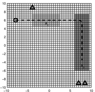
Figure 1: Simulation scenario in the Range-Only Tracking Demonstration. Circle denotes the starting location of the target, triangles the locations of the sensors and the dashed line the trajectory of the target. Inside the shaded areas the noise field has spatial correlations.

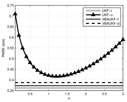
Figure 2: Range-Only Tracking: RMSE values for tracking the position of the target on a typical simulation run. The different standard deviation values used for UKF-o are on X-axis.

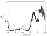
(a) $\sigma^{2}_{1,1}$

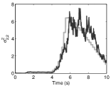
(b) $\sigma^{2}_{2,2}$

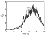
(c) $\sigma^{2}_{3,3}$

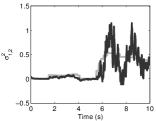
(d) $\sigma^{2}_{1,2}$

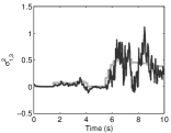
(e) $\sigma^{2}_{1,3}$

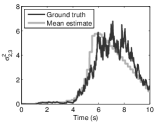
(f) $\sigma^{2}_{2,3}$

Figure 3: Range-Only Tracking: Estimates of $\Sigma_{k}$ with VBAUKF-f. Smoother estimates can be obtained by tuning $\rho$ to be larger, but that introduces more lag to estimates.

3.2 Multi-Sensor Bearings Only Tracking

As an example, we consider the classical multi-sensor bearings only tracking problem with coordinated turning model, where the state $x=(u,\dot{u},v,\dot{v},\omega)$ contains the 2d location $(u,v)$ and the corresponding velocities $(\dot{u},\dot{v})$ as well as the turning rate $\omega$ of the target. The dynamic model and the measurement models for sensors $i=1,\ldots,4$ are given as:

$$\begin{split}x_{k}&=\begin{pmatrix}1&\frac{\sin(\omega\Delta t)}{\omega}&0&-\left(\frac{1-\cos(\omega\Delta t)}{\omega}\right)&0\\ 0&\cos(\omega\Delta t)&0&-\sin(\omega\Delta t)&0\\ 0&\frac{1-\cos(\omega\Delta t)}{\omega}&1&\frac{\sin(\omega\Delta t)}{\omega}&0\\ 0&\sin(\omega\Delta t)&0&\cos(\omega\Delta t)&0\\ 0&0&0&0&1\end{pmatrix}x_{k-1}+q_{k-1}\\ y_{k}&=\arctan\left(\frac{v_{k}-s^{i}_{v}}{u_{k}-s^{i}_{u}}\right)+r_{i,k},\qquad i=1,\ldots,4,\end{split}$$ (21)

where $q_{k}\sim\mathrm{N}(0,Q)$ is the process noise and $r_{k}=(r_{k,1},\ldots,r_{k,4})$ are the measurement noises of sensors with joint distribution $r_{k}\sim\mathrm{N}(0,\Sigma_{k})$, where $\Sigma_{k}$ is unknown and time varying.

We simulated a trajectory and measurements from the model and applied different filters to it. We tested various Gaussian integration based methods (VB-AEKF, VB-AUKF, VB-ACKF, VB-AGHKF) and because the results were quite much the same with different Gaussian integration methods (though VB-AEKF was a bit worse than the others), we only present the results obtained with VB-ACKF. Figure 4 shows the simulated trajectory and the VB-ACKF results with the full covariance estimation. In the simulation, the variances of the measurement noises as well as the cross-correlations varied smoothly over time. The simulated measurements are shown in Figure 5.

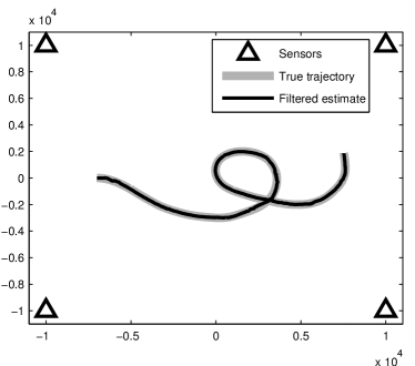
Figure 4: The simulated trajectory and the estimate obtained with VB-ACKF.

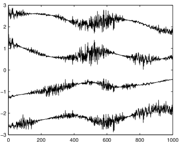
Figure 5: The simulated measurements.

Figure 6 shows the root mean squared errors (RMSEs) for the following methods:

• CKF-t: CKF with the true covariance matrix.

• CKF-o: CKF with a diagonal covariance matrix with diagonal elements given by the value on the $x$-axis.

• VBCKF-f: CKF with full covariance estimation.

• VBCKF-d: CKF with diagonal covariance estimation.

As can be seen from the figure, the results of filters with covariance estimation are indeed better than the results of any filter with fixed diagonal covariance matrix. The filter with the known covariance matrix gives the lowest error, as would be expected, and the filter with full covariance estimation gives a lower error than the filter with diagonal covariance estimation.

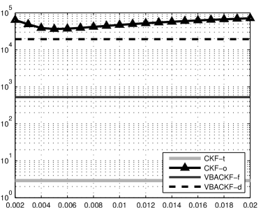
Figure 6: Root mean squared errors (RMSEs) for different methods.

4 Conclusion and Discussion

In this paper, we have presented a variational Bayes and Gaussian filtering based algorithm for joint estimation of state and time-varying noise covariances in non-linear state space models. The performance of the method has been illustrated in simulated applications.

There are several extensions that could be considered as well. For instance, we could try to estimate the process noise covariance in the model. However, it is not as easy as it sounds, because the process noise covariance does not appear in the equations in such simple conjugate form as the measurement noise covariance. Another natural extension would be the case of smoothing (cf. [4]). Unfortunately the current dynamic model makes things challening, because we do not know the actual transition density at all. This makes the implementation of a Rauch–Tung–Striebel type of smoother impossible—although a simple smoothing estimate for the state can be obtained by simply running the RTS smoother over the state estimates while ignoring the noise covariance estimates completely. However, it would be possible to construct an approximate two-filter smoother for the full state space model, but even in that case we need to put some more constraints to the model, for example, assume that the covariance dynamics are time-reversible.

References

- [1] A. H. Jazwinski, Stochastic Processes and Filtering Theory, Academic Press, 1970.
- [2] P. Maybeck, Stochastic Models, Estimation and Control, Volume 2, Academic Press, 1982.
- [3] S. Särkkä, A. Nummenmaa, Recursive noise adaptive Kalman filtering by variational Bayesian approximations, IEEE Transactions on Automatic Control 54(3) (2009) 596–600.
- [4] R. Piché, S. Särkkä, J. Hartikainen, Recursive outlier-robust filtering and smoothing for nonlinear systems using the multivariate Student-t distribution, in: Proceedings of MLSP, 2012.
- [5] G. Agamennoni, J. Nieto, E. Nebot, An outlier-robust Kalman filter, in: IEEE Int. Conf. on Robotics and Automation (ICRA), 2011, pp. 1551–1558. doi:10.1109/ICRA.2011.5979605.
- [6] T. S. Jaakkola, Tutorial on variational approximation methods, in: M. Opper, D. Saad (Eds.), Advanced Mean Field Methods – Theory and Practice, MIT Press, 2001, pp. 129–159.
- [7] M. J. Beal, Variational algorithms for approximate Bayesian inference, Ph.D. thesis, Gatsby Computational Neuroscience Unit, University College London (2003).
- [8] H. Lappalainen, J. W. Miskin, Ensemble learning, in: M. Girolami (Ed.), Advances in Independent Component Analysis, Springer-Verlag, 2000, pp. 75–92.
- [9] K. Ito, K. Xiong, Gaussian filters for nonlinear filtering problems, IEEE Transactions on Automatic Control 45 (5) (2000) 910–927.
- [10] Y. Wu, D. Hu, M. Wu, X. Hu, A numerical-integration perspective on Gaussian filters, IEEE Transactions on Signal Processing 54 (8) (2006) 2910–2921.
- [11] S. J. Julier, J. K. Uhlmann, H. F. Durrant-Whyte, A new method for the nonlinear transformation of means and covariances in filters and estimators, IEEE Transactions on Automatic Control 45 (3) (2000) 477–482.
- [12] I. Arasaratnam, S. Haykin, Cubature Kalman filters, IEEE Transactions on Automatic Control 54 (6) (2009) 1254–1269.
- [13] M. Nørgaard, N. K. Poulsen, O. Ravn, New developments in state estimation for nonlinear systems, Automatica 36 (11) (2000) 1627 – 1638.
- [14] T. Lefebvre, H. Bruyninckx, J. D. Schutter, Comment on ”a new method for the nonlinear transformation of means and covariances in filters and estimators” [and authors’ reply], IEEE Transactions on Automatic Control 47 (8) (2002) 1406–1409.
- [15] M. P. Deisenroth, M. F. Huber, U. D. Hanebeck, Analytic moment-based Gaussian process filtering, in: Proceedings of the 26th International Conference on Machine Learning, 2009.
- [16] V. Smidl, A. Quinn, The Variational Bayes Method in Signal Processing, Springer, 2006.
- [17] M. J. Beal, Z. Ghahramani, The variational Kalman smoother, Tech. Rep. TR01-003, Gatsby Unit (2001).
- [18] H. Valpola, M. Harva, J. Karhunen, Hierarchical models of variance sources, Signal Processing 84(2) (2004) 267–282.
- [19] G. Storvik, Particle filters in state space models with the presence of unknown static parameters, IEEE Transactions on Signal Processing 50(2) (2002) 281–289.
- [20] P. M. Djuric, J. Miguez, Sequential particle filtering in the presence of additive Gaussian noise with unknown parameters, in: Proceedings of the IEEE International Conference on Acoustics, Speech, and Signal Processing, Orlando, FL, 2002.
- [21] S. Särkkä, On sequential Monte Carlo sampling of discretely observed stochastic differential equations, in: Proceedings of the Nonlinear Statistical Signal Processing Workshop, 2006, [CDROM].
- [22] X. R. Li, Y. Bar-Shalom, A recursive multiple model approach to noise identification, IEEE Transactions on Aerospace and Electronic Systems 30(3).
- [23] A. Gelman, J. B. Carlin, H. S. Stern, D. R. Rubin, Bayesian Data Analysis, Chapman & Hall, 1995.
- [24] J. H. Kotecha, P. M. Djuric, Gaussian particle filtering, IEEE Transactions on Signal Processing 51 (10) (2003) 2592–2601.