Ascertaining the Uncertainty Relations via Quantum Correlations

Abstract

We propose a new scheme to express the uncertainty principle in form of inequality of the bipartite correlation functions for a given multipartite state, which provides an experimentally feasible and model-independent way to verify various uncertainty and measurement disturbance relations. By virtue of this scheme the implementation of experimental measurement on the measurement disturbance relation to a variety of physical systems becomes practical. The inequality in turn also imposes a constraint on the strength of correlation, i.e. it determines the maximum value of the correlation function for two-body system and a monogamy relation of the bipartite correlation functions for multipartite system.

The uncertainty principle lies at the heart of quantum mechanics and is one of the most fundamental features which distinguish it from the classical mechanics. The original form, $p_{1}q_{1}\sim h$, stems from a heuristic discussion of Heisenberg on Compton scattering [1] where $p_{1}$, $q_{1}$ are the determinable precisions of position and momentum, $h$ is the Planck constant. A generalization to arbitrary pairs of observables is $\Delta{A}\Delta{B}\geq|\langle[A,B]\rangle|/2$, where the standard deviation is $\Delta{X}=(\langle X^{2}\rangle-\langle X\rangle^{2})^{1/2}$, $X=A\ \text{or}\ B$, $\langle\cdots\rangle$ stands for expectation value, and the commutator is defined as $[A,B]\equiv AB-BA$. This is the usually called Heisenberg-Robertson uncertainty relation [2]. A more stronger version is the Robertson-Schrödinger uncertainty relation [3] which takes the form of $(\Delta{A})^{2}(\Delta{B})^{2}\geq(\langle\{A,B\}\rangle/2-\langle A\rangle\langle B\rangle)^{2}+|\langle[A,B]\rangle|^{2}/4$ where the anticommutator is defined as $\{A,B\}\equiv AB+BA$.

Note that in the form involving standard deviations, the uncertainty relation represents the property of the ensemble of arbitrary quantum state in Hilbert space and does not concern with the specific measurements. Thus such uncertainty relation is not related to the precision of measurement on one observable and the disturbance to its conjugate.

If we assume $\epsilon(A)$ to be the precision of the measurement on $A$ and $\eta(B)$ to be the disturbance of the same measurement on $B$, the Heisenberg-type relation with regard to measurement and disturbance would read

$$\epsilon(A)\eta(B)\geq\frac{1}{2}|\langle[A,B]\rangle|\;.$$ (1)

In recently, Ozawa found that the this form of measurement disturbance relation (MDR) (1) is not a universal one, and a new MDR was proposed [4], which are thought to be generally valid, i.e.

$$\epsilon(A)\eta(B)+\epsilon(A)\Delta B+\Delta A\,\eta(B)\geq\frac{1}{2}|\langle[A,B]\rangle|\;.$$ (2)

Eq.(2) is of fundamental importance, for example, it leads to a totally different accuracy limit $\epsilon(A)$ for non-disturbing measurements ($\eta(B)=0$) comparing to the Heisenberg-type MDR. In quantum information science, the uncertainty principle in general is also crucial to the security of certain protocols in quantum cryptography [5], and additionally, it plays an important role in the quantum metrology [6].

Despite the importance of the uncertainty principle, only the uncertainty relation in form of standard deviations has been well verified in various situations, e.g., see [7] and the references therein. Experiments concerning both Heisenberg-type and Ozawa’s MDRs have just been performed with neutrons [8] and photons [9]. For neutrons in a given polarization state, the error and disturbance can be statistically determined based on a method proposed by Ozawa [10]. In the photon experiment, the weak measurement model introduced in [11] was employed for the measurement. Large samples of data is necessary due to the sensitivity to the measurement strength of a weak measurement process which is used for gathering information of the system prior to the actual measurement [12]. The results of [8] and [9] exhibit the validation of Ozawa’s MDR but rather the Heisenberg-type. Since the uncertainty principle limits our ultimate ability to reduce noise when gaining information from the state of a physical system, its experimental verification in various systems and different measurement interactions is still an important subject.

Here in this work, we present such a general scheme from which both the uncertainty relation and MDR turn to the forms involving only bipartite correlation functions. In this formalism, whilst the uncertainty relation becomes an inequality imposed on the correlation functions of bipartite states, the different forms of MDRs transform into strong constraints on the shareability (monogamy) of the bipartite correlations in multipartite state. This directly relates the key element of quantum information, i.e., the nonlocal correlation, with the fundamental principle of quantum mechanics, i.e., uncertainty principle, in a quantitative way. And most importantly, it enables us to test the MDRs in a variety of physical systems.

To test the validity of the various MDRs, one has to measure the physical observable quantities for which the different MDRs exhibit distinct responses. Here we present our method of constructing such quantities for qubit systems. Although the generalization to arbitrary systems is not trivial, the various MDRs have already shown the essential differences in two-dimensional Hilbert spaces within our scheme. The qubit systems include spin 1/2 particle, polaizations of photons, two level atoms, etc. For the sake of convenience we take the measurable observables to be the spin components. A measurement of spin along arbitrary vector $\vec{a}$ in three dimensional Euclidean space can be represented by the following operator

$$A=\vec{\sigma}\cdot\vec{a}=|\vec{a}|\vec{\sigma}\cdot\vec{n}_{a}\;.$$ (3)

Here $\vec{\sigma}=(\sigma_{x},\sigma_{y},\sigma_{z})$ are Pauli matrices, $\vec{n}_{a}=\vec{a}/|\vec{a}|$, and a general commutative relation holds for such operators

$$[A,B]=2iC\;,$$ (4)

where $B=\vec{\sigma}\cdot\vec{b}$, $C=\vec{\sigma}\cdot\vec{c}$, $\vec{c}=\vec{a}\times\vec{b}$. Let $|n^{\pm}_{p}\rangle$ be the two eigenvectors of operator $P=\vec{\sigma}\cdot\vec{n}_{p}$ with eigenvalues $\pm 1$, the following complete relations hold

$$|n^{+}_{p}\rangle\langle n^{+}_{p}|+|n^{-}_{p}\rangle\langle n^{-}_{p}|=1\;,\;|n^{+}_{p}\rangle\langle n^{+}_{p}|-|n^{-}_{p}\rangle\langle n^{-}_{p}|=\vec{\sigma}\cdot\vec{n}_{p}=P\;.$$ (5)

Here $\vec{n}_{p}$ is a unit vector, $|n_{p}^{\pm}\rangle\langle n_{p}^{\pm}|\equiv P^{\pm}$ are the projection operators. Using the Schmidt decomposition, any bipartite pure state is unitarily equivalent to the state [13]: $|\psi_{12}\rangle=\alpha|+\rangle|+\rangle+\beta|-\rangle|-\rangle$ where $|\alpha|^{2}+|\beta|^{2}=1$, and $\alpha\geq 0$, $\beta\geq 0$. The correlation function between two operators $A$ and $B$ for arbitrary quantum state $|\psi\rangle$ is defined as $E(A_{1},B_{2})=\langle\psi|A_{1}\otimes B_{2}|\psi\rangle$. Here the subscripts of $A$, $B$ stand for the corresponding partite which they are acting.

For the Robertson-Schrödinger uncertainty relation we have the following theorem:

Theorem 1

The Robertson-Schrödinger uncertainty relation imply the following inequality on the correlation functions of arbitrary bipartite quantum state

$$\left|E(A_{1},P_{2})\vec{b}-E(B_{1},P_{2})\vec{a}\right|^{2}+\left|E(C_{1},P_{2})\right|^{2}\leq S^{2}\;,$$

where $X_{i}=\vec{\sigma}_{i}\cdot\vec{x}$, $X=A,\ B,\ \text{or}\ C$, $\vec{c}=\vec{a}\times\vec{b}$, $P_{i}=\vec{\sigma}_{i}\cdot\vec{n}_{p}$, $\vec{n}_{p}$ is unit vector, $i=1,2$ denote the corresponding partite, $S$ is the parallelogram area formed by $\vec{a}$, $\vec{b}$.

This theorem indicates that the correlation functions between one specific operator ($P$) and two other operators ($A$, $B$) and their commutator ($C$) in bipartite states are constrained by the area of parallelogram formed with $\vec{a}$ and $\vec{b}$. The maximal attainable value of the bipartite correlation function is $E(A_{1},A_{2})=|\vec{a}|^{2}$ which is the area of a square with length $|\vec{a}|$. A proof of this theorem is given in Appendix A.

As for the MDR, it is a subtle problem in quantum theory. In order to detect the influence (disturbance) on quantity $B$ introduced in measuring $A$, one needs to measure $B$ before and after the measurement on $A$. If the initial state is not $B$’s eigenstate, the acquisition of information on $B$ prior to the measurement $A$ will inevitably change the the initial state and makes the subsequent measurement process irrelevant to the initial state. To illustrate this, a simple measurement scheme is presented in Fig.1 where the measurement is performed via the interaction of the signal system $|\psi_{1}^{\pm}\rangle$ with a meter system $|\psi_{3}\rangle$ [11].

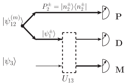
Figure 1: Illustration of the detection of measurement precision and disturbance. P, D, M stand for the function of projection, disturbance, and measuring. A meeter system $|\psi_{3}\rangle$ interacts with the signal state $|\psi_{1}^{\pm}\rangle$ which is prepared by projecting a bipartite entangled state $|\psi_{12}^{(m)}\rangle$ at P. The measurement result can be obtained from M, and the measurement disturbance on signal $|\psi_{1}^{\pm}\rangle$ will be detected at D.

The Ozawa’s precision and disturbance quantities in Eq.(2) are defined as [4]

$$\epsilon(A)^{2} \equiv \langle[U^{{\dagger}}_{13}(I_{1}\otimes M_{3})U_{13}-A_{1}\otimes I_{3}]^{2}\rangle\;,$$ (6)

$$\eta(B)^{2} \equiv \langle[U^{{\dagger}}_{13}(B_{1}\otimes I_{3})U_{13}-B_{1}\otimes I_{3}]^{2}\rangle\;.$$ (7)

Here the expectation values in Eqs.(6, 7) are evaluated with the same compound state $|\psi_{1}\rangle|\psi_{3}\rangle$, where $|\psi_{1}\rangle$ can be arbitrary, i.e., $|\psi_{1}^{\pm}\rangle$; $|\psi_{3}\rangle$ is the quantum state of the measurement apparatus; $U_{13}$ is a unitary measurement interaction. If the measurement process is carried out via spin dependent interaction with a qubit state (partite 3) and regarding the measurement read out of the spin of partite 3 to be the measurement result of the signal state $|\psi_{1}\rangle$, we can have $M_{3}\to A_{3}$. It is obvious that in determining $\eta(B)$ (Eq.(7)), we have to measure $B_{1}$ before and after the measurement interaction $U_{13}$.

Our procedure to settle the measurement problem under Ozawa’s defintions goes as follows. Suppose we want to measure the MDR with respect to any given pair of spin components of $A_{1}=\vec{\sigma}_{1}\cdot\vec{a}$ and $B_{1}=\vec{\sigma}_{1}\cdot\vec{b}$ for arbitrary state $|\psi_{1}\rangle$. This state can be prepared via the following entangled state

$$|\psi_{12}^{(m)}\rangle=\frac{1}{\sqrt{2}}\left(|+\rangle_{c}|-\rangle_{c}+(-1)^{m}|-\rangle_{c}|+\rangle_{c}\right)\;.$$ (8)

Here, $m\in\{0,1\}$; $\vec{c}=\vec{a}\times\vec{b}$ and $|\pm\rangle_{c}$ are the spin eigenstates along $\vec{c}$ ($|\pm\rangle$ stand for the eigenstates along $z$ if not specified). Without loss of generality, we can set the $\vec{a}$-$\vec{b}$ plane as $x$-$z$ plane then $\vec{c}$ is along the $y$ axis

$$|\psi_{12}^{(1)}\rangle = \frac{1}{\sqrt{2}}\left(|+-\rangle-|-+\rangle\right)\;,$$ (9)

$$|\psi_{12}^{(0)}\rangle = \frac{1}{\sqrt{2}}\left(|++\rangle+|--\rangle\right)\;.$$ (10)

$|\psi_{12}^{(m)}\rangle$ have the following property

$$V_{1}\otimes V^{-1}_{2}|\psi_{12}^{(m)}\rangle=(-1)^{m}|\psi_{12}^{(m)}\rangle\;,\;m\in\{0,1\}\;,$$ (11)

where $V_{i}=\vec{\sigma}_{i}\cdot\vec{v}$ is an operator acting on the $i$th partite and $\vec{v}$ is a unit vector in the $\vec{a}$-$\vec{b}$ (i.e., $x$-$z$) plane. With the definition of projection operators in Eq.(5), an arbitrary quantum state ($|\psi_{1}\rangle$) of partite 1 can be obtained via a projective measurement P on partite 2 (see Fig.1)

$$|\psi_{1}^{\pm}\rangle = \frac{{}_{2}\langle n_{p}^{\pm}|\psi_{12}^{(m)}\rangle}{|_{2}\langle n_{p}^{\pm}|\psi_{12}^{(m)}\rangle|}\;.$$ (12)

Here in the present situation $|_{2}\langle n_{p}^{\pm}|\psi_{12}^{(m)}\rangle|=1/\sqrt{2}$ and the arbitrariness of $|\psi_{1}^{\pm}\rangle$ is guaranteed by the arbitrariness of $\vec{n}_{p}$.

The measurement precision of quantity $A$ for quantum state $|\psi_{1}^{\pm}\rangle$ and the corresponding disturbance on another quantity $B$ now can be written as

$$\epsilon^{\pm}(A)^{2}=\langle\psi_{3}|\langle\psi_{1}^{\pm}|\left[U_{13}^{{\dagger}}(I_{1}\otimes A_{3})U_{13}-A_{1}\otimes I_{3}\right]^{2}|\psi_{1}^{\pm}\rangle|\psi_{3}\rangle\;,$$ (13)

$$\eta^{\pm}(B)^{2}=\langle\psi_{3}|\langle\psi_{1}^{\pm}|\left[U_{13}^{{\dagger}}(B_{1}\otimes I_{3})U_{13}-B_{1}\otimes I_{3}\right]^{2}|\psi_{1}^{\pm}\rangle|\psi_{3}\rangle\;.$$ (14)

With these definitions, we can derive the following relation (see the Appendix B)

$$|\vec{a}|^{2}+|\vec{b}|^{2}-(-1)^{m}[E(A_{2},A_{3})+E(B_{1},B_{2})]$$ (15)

$$= \frac{1}{4}\left[\epsilon^{+}(A)^{2}+\eta^{+}(B)^{2}+\epsilon^{-}(A)^{2}+\eta^{-}(B)^{2}\right]\;,$$

where the correlation function $E(X_{i},X_{j})=\langle\psi_{123}|X_{i}\otimes X_{j}|\psi_{123}\rangle$, $X=A\ \text{or}\ B$, $|\psi_{123}\rangle\equiv U_{13}|\psi_{12}^{(m)}\rangle|\psi_{3}\rangle$, $i,j\in\{1,2,3\}$, the subscripts of operators stand for the corresponding partite which they are acting. The precision and disturbance of the measurement now are directly related to the bipartite correlation functions of a tripartite state. Eq.(15) is universally valid regardless of the measurement interaction $U_{13}$ which brings about the tripartite state.

For arbitrary given state $|\psi_{1}^{\pm}\rangle$, the Heisenberg-type and Ozawa’s MDRs read

$$\epsilon^{\pm}(A)\eta^{\pm}(B)\geq\frac{1}{2}|\langle\psi_{1}^{\pm}|[A,B]|\psi_{1}^{\pm}\rangle|\;,$$ (16)

$$\epsilon^{\pm}(A)\eta^{\pm}(B)+\epsilon^{\pm}(A)\Delta^{\pm}(B)+\eta^{\pm}(B)\Delta^{\pm}(A)\geq\frac{1}{2}|\langle\psi_{1}^{\pm}|[A,B]|\psi_{1}^{\pm}\rangle|\;.$$ (17)

An intuitive view of the above equations tells that the allowed regions for $\epsilon$ and $\eta$ lie above the hyperbolic curves of $\epsilon^{\pm}(A)$ and $\eta^{\pm}(B)$ in the quadrant I. The constraints Eqs.(16,17) are then transferred to the bipartite correlation functions via Eq.(15). Thus we have the following theorem

Theorem 2

For $A=\vec{\sigma}\cdot\vec{a}$, $B=\vec{\sigma}\cdot\vec{b}$, a tripartite state can be obtained by interacting one partite of $|\psi_{12}^{(m)}\rangle$ with a third partite 3. The Heisenberg-type and Ozawa’s MDRs imply the following different relations on the resulted tripartite state

$$E(A_{2},A_{3})+E(B_{1},B_{2})\leq|\vec{a}|^{2}+|\vec{b}|^{2}-\kappa_{h,o}|\vec{n}_{p}\cdot(\vec{a}\times\vec{b})|\;.$$ (18)

Here $E(X_{i},X_{j})$ are the bipartite correlation functions of the tripartite state, $\kappa_{h}=1$ and $\kappa_{o}=(\sqrt{2}-1)^{2}$ for Heisenberg-type and Ozawa’s MDR respectively, $\vec{n}_{p}$ is an arbitrary unit vector.

The proof of Theorem 2 is presented in Appendix C. From Theorem 1 we know that $|\vec{a}|^{2}$ and $|\vec{b}|^{2}$ are the maximum values of $E(A_{2},A_{3})$ and $E(B_{1},B_{2})$ in bipartite states. Now due to Theorem 2 the maximum of the sum of the two bipartite correlations in the tripartite state is reduced by an amount proportional to the volume of the parallelepiped with edges $\vec{a}$, $\vec{b}$, and $\vec{n}_{p}$.

The experiments to test the validity of the MDRs become straightforward due to Theorem 2. Here we present an example of the measurement model of qubit system with the measurement interaction $U_{13}$ being the CNOT gate [11] within our method. Suppose we want to measure the precision of $Z=\sigma_{z}$ and the disturbance on $X=\sigma_{x}$ for an arbitrary qubit state $|\psi_{1}\rangle$. Following Theorem 2, on choosing $|\psi_{12}^{(1)}\rangle=\frac{1}{\sqrt{2}}(|++\rangle+|--\rangle)$, the measurement interaction CNOT gate between one partite of $|\psi_{12}^{(1)}\rangle$ and the meeter system $|\psi_{3}\rangle=\cos\theta_{3}|+\rangle+\sin\theta_{3}|-\rangle$ will lead to the following tripartite state

$$|\psi_{123}\rangle = \frac{1}{\sqrt{2}}[|++\rangle(\cos\theta_{3}|+\rangle+\sin\theta_{3}|-\rangle)+$$ (19)

$$\hskip 22.76228pt|--\rangle(\cos\theta_{3}|-\rangle+\sin\theta_{3}|+\rangle)]\;.$$

According to Theorem 2, the Heisenberg-type and Ozawa’s MDRs impose the following constraints on the bipartite correlation functions of $|\psi_{123}\rangle$

$$\text{Heisenberg-type MDR: }\;E(Z_{2},Z_{3})+E(X_{1},X_{2}) \leq 2-|\cos\theta_{p}|\;,$$ (20)

$$\text{Ozawa's MDR: }\;E(Z_{2},Z_{3})+E(X_{1},X_{2}) \leq 2-(\sqrt{2}-1)^{2}|\cos\theta_{p}|\;,$$ (21)

for arbitrary $\theta_{p}$, the angle between $\vec{n}_{p}$ and $\vec{c}$. The tightest bound happens when $\theta_{p}=0$. Thus a measurement of bipartite correlation function of $E(Z_{2},Z_{3})$, $E(X_{1},X_{2})$ in the tripartite state would be capable to verify the Heisenberg-type and Ozawa’s MDR (see Fig.2). That is the Heisenberg-type MDR will be violated provided that the experimental result agrees with the solid line of $E(Z_{2},Z_{3})+E(X_{1},X_{2})$ in Fig.2.

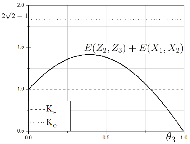
Figure 2: The demonstration of Heisenberg-type and Ozawa’s MDR with measurement precision of $A=Z$ and its disturbance on $B=X$. Here $K_{H,O}$ are the upper bound imposed by Heisenberg-type and Ozawa’s MDR at $\theta_{p}=0$ respectively. The sum $E(Z_{2},Z_{3})+E(X_{1},X_{2})$ surpasses the limit imposed by Heisenberg-type MDR.

From the above example, the procedure of our scheme can be summarized as: (1) prepare a bipartite entangled state, (2) interact one partite of the entangled state with a third partite, and (3) measure the bipartite correlation functions of the resulted tripartite state. The generation of the bipartite entangled state has already been realized in various systems, e.g. photons [14, 15], atoms [16, 17], and high energy particles [18, 19]. The further interaction of one partite of the entangled state with a third partite can also be arbitrary, i.e., elastic or inelastic collisions, or via optical cavities, etc. More importantly, we need only to measure the bipartite correlation functions of the obtained tripartite state rather than the measurement precision and disturbance, which may not be easy to quantify for some types of measurement interactions. Hence, our scheme could be applied to a large number of systems in the verification of the MDRs.

In addition to a clear discrimination between the Heisenberg-type and Ozawa’s MDRs, a more important physical consequence of the Theorem 2 is that it reveals a monogamy relation on Bell correlations [20, 21, 22] in the tripartite entangled state. According to the Theorem 2, when measuring the precision of $B$ and the disturbance it imposes on $A$, we will have

$$|E(B_{2},B_{3})+E(A_{1},A_{2})|\leq|\vec{a}|^{2}+|\vec{b}|^{2}-\kappa_{h,o}|\vec{n}_{p}\cdot(\vec{a}\times\vec{b})|\;,$$ (22)

Introducing two new vectors $\vec{a}\,^{\prime}=\frac{1}{2}(\vec{a}+\vec{b})$ , $\vec{b}^{\prime}=\frac{1}{2}(\vec{b}-\vec{a})$, we can similarly define $A^{\prime}=\vec{\sigma}\cdot\vec{a}^{\prime}$, $B^{\prime}=\vec{\sigma}\cdot\vec{b}^{\prime}$. Following the definition of correlation function in Eq.(15), we can get

$$E(A_{i},A_{j}) = E(A_{i},A^{\prime}_{j})-E(A_{i},B^{\prime}_{j})\;,$$ (23)

$$E(B_{i},B_{j}) = E(B_{i},A^{\prime}_{j})+E(B_{i},B^{\prime}_{j})\;.$$ (24)

Adding Eq.(18) and Eq.(22), and taking Eqs.(23,24), we have

$$\left|E(A_{2},A^{\prime}_{3})-E(A_{2},B^{\prime}_{3})+E(B_{2},A^{\prime}_{3})+E(B_{2},B^{\prime}_{3})+\right.$$

$$\left.\hskip 2.84544ptE(A_{1},A^{\prime}_{2})-E(A_{1},B^{\prime}_{2})+E(B_{1},A^{\prime}_{2})+E(B_{1},B^{\prime}_{2})\hskip 5.69046pt\right|\leq 2K_{H,O}\;.$$ (25)

where $K_{H,O}=|\vec{a}|^{2}+|\vec{b}|^{2}-\kappa_{h,o}|\vec{n}_{p}\cdot(\vec{a}\times\vec{b})|$. When $|\vec{a}|=|\vec{b}|=1$, $\vec{a}\perp\vec{b}$, Eq.(25) leads to the sum of two particular CHSH type correlations [23]

$$\left|B_{\text{CHSH}}^{(23)}+B_{\text{CHSH}}^{(12)}\right|\leq 2\sqrt{2}K_{H,O}\;.$$ (26)

Here $B_{\text{CHSH}}^{(ij)}=E(A_{i},A^{\prime}_{j})-E(A_{i},B^{\prime}_{j})+E(B_{i},A^{\prime}_{j})+E(B_{i},B^{\prime}_{j})$. The tightest bound also happens when $\theta_{p}=0$, which lead the following

$$\text{Heisenberg-type MDR: }\;\left|B_{\text{CHSH}}^{(23)}+B_{\text{CHSH}}^{(12)}\right| \leq 2\sqrt{2}\;,$$ (27)

$$\text{Ozawa's MDR: }\;\left|B_{\text{CHSH}}^{(23)}+B_{\text{CHSH}}^{(12)}\right| \leq 2\sqrt{2}(2\sqrt{2}-1)\;.$$ (28)

The above monogamy relations on quantum nonlocality are direct results of the MDRs according to our theorem. Note, there are also discussions in the literature on Bell correlations based on the entropic measures of uncertainty relation [24, 25].

It should be noted that the definitions of measurement precision and disturbance in Eqs.(6,7) by Ozawa involve the comparisons of the same physical observable before and after the measurement, thus base on practical physical motivations. However, the exact definitions that capture the full physical contents of the measurement error and disturbance are still under study [26, 27, 28]. Nevertheless, Ozawa’s definitions and the resulted MDRs may be regarded as one of the best attempts to capture the quantitative descriptions of the measurement and its back action in quantum mechanics. The method we presented just provides a powerful tool to study the physical consequences of the MDRs which is meaningful in judging their usefulness. For example, our method transforms the MDRs into inequalities of correlation functions of tripartite entangled state. In this way the importance of the MDRs manifests in their connections with the quantum entanglement which is a key physical resource in quantum information science and has a close relation with quantum metrology [6]. Meanwhile, in principle the idea of our scheme may also be applied to other definitions of the error and disturbance. This would enable the method to examine the meaningfulness of the variant definitions.

In conclusion, we proposed in this work a general scheme to express the uncertainty principle in terms of bipartite correlation functions, by which the essential differences between the MDRs are characterized by the inequalities constraining the correlation functions of multipartite state. This not only builds a bridge between the MDRs and the quantum entanglement but also provides a way to study the direct physical consequences of such fundamental relations. The resulted inequalities reveal that both the strength and the shareability (monogamy) of the quantum correlation are determined by the uncertainty principle. Further studies on the uncertainty relation and MDRs with, e.g., atoms, ions, or even high energy particles become possible due to our scheme. The connections between MDRs and entanglement revealed in our scheme may also shed new light on the the studies of the relations between the MDRs and the quantum cryptography, quantum metrology, etc.

Note: after the completion of the manuscript, there has been some progress in the study of MDRs, i.e., [29],[30],etc. Our method may apply to such cases as well and these MDRs would also give distinct constraints on quantum correlations [31].)

Acknowledgments

This work was supported in part by the National Natural Science Foundation of China(NSFC) under the grants 10935012, 11121092, 11175249 and 11205239.

Appendix

Appendix A Proof of theorem 1

Proof of the equation of theorem 1:

$$\left|E(A_{1},P_{2})\vec{b}-E(B_{1},P_{2})\vec{a}\right|^{2}+\left|E(C_{1},P_{2})\right|^{2}\leq S^{2}\;.$$

Proof: Following the definition of the standard deviation, the Robertson-Schrödinger uncertainty relation takes the following form

$$(\langle A^{2}\rangle-\langle A\rangle^{2})(\langle B^{2}\rangle-\langle B\rangle^{2})\geq\left(\frac{1}{2}\langle AB+BA\rangle-\langle A\rangle\langle B\rangle\right)^{2}+\frac{1}{4}\left|\langle[A,B]\rangle\right|^{2}\;.$$ (29)

With the definition of operators as in Eq.(3) and the basic commutator Eq.(4), Eq.(29) can be written as

$$|\vec{a}|^{2}|\vec{b}|^{2}-\langle A\rangle^{2}|\vec{b}|^{2}-\langle B\rangle^{2}|\vec{a}|^{2} \geq (\vec{a}\cdot\vec{b})^{2}-2(\vec{a}\cdot\vec{b})\langle A\rangle\langle B\rangle+\langle C\rangle^{2}\;.$$

After rearranging the terms, we have

$$|\langle A\rangle\vec{b}-\langle B\rangle\vec{a}|^{2}+\langle C\rangle^{2}\leq|\vec{a}|^{2}|\vec{b}|^{2}-(\vec{a}\cdot\vec{b})^{2}=S^{2}\;.$$

The right hand side of the inequality is just the determinant of Gram matrix of the vector $\vec{a}$, $\vec{b}$, which is the square of area of parallelogram formed by $\vec{a}$, $\vec{b}$. The expectation value is evaluated for certain quantum state which can be prepared by projecting one partite of the bipartite entangled state onto specific quantum state. For example, for the entangled state $|\psi_{12}\rangle=\alpha|+\rangle_{1}|+\rangle_{2}+\beta|-\rangle_{1}|-\rangle_{2}$, by projecting the partite 2 onto a specific state $|n_{p}^{+}\rangle_{2}=\cos\frac{\theta}{2}|+\rangle+e^{i\phi}\sin\frac{\theta}{2}|-\rangle$ (Eigenstate of $\vec{\sigma}_{2}\cdot\vec{n}_{p}$ where $\vec{n}_{p}=(\sin\theta\cos\phi,\sin\theta\sin\phi,\cos\theta)$), we can get arbitrary quantum state $|\psi_{1}^{+}\rangle$

$$|\psi_{1}^{+}\rangle=\frac{{}_{2}\langle n_{p}^{+}|\psi_{12}\rangle}{|\,_{2}\langle n_{p}^{+}|\psi_{12}\rangle|}=\frac{1}{|\,_{2}\langle n_{p}^{+}|\psi_{12}\rangle|}\left(\alpha\cos\frac{\theta}{2}|+\rangle+e^{-i\phi}\beta\sin\frac{\theta}{2}|-\rangle\right)\;.$$ (30)

Similar expression holds for $|\psi_{1}^{-}\rangle$ when projecting with $|n_{p}^{-}\rangle_{2}$. The uncertainty relation holds for arbitrary state, so for $|\psi_{1}^{\pm}\rangle$

$$|\langle A\rangle\vec{b}-\langle B\rangle\vec{a}|^{2}+\langle C\rangle^{2}\leq S^{2}$$ (31)

$$\Rightarrow |\langle\psi_{1}^{\pm}|A_{1}|\psi_{1}^{\pm}\rangle\vec{b}-\langle\psi_{1}^{\pm}|B_{1}|\psi_{1}^{\pm}\rangle\vec{a}|^{2}+\langle\psi_{1}^{\pm}|C_{1}|\psi_{1}^{\pm}\rangle^{2}\leq S^{2}\;.$$

Here the subscript $1$ standards for partite 1. Multiplying $|\,_{2}\langle n_{p}^{\pm}|\psi_{12}\rangle|^{2}$ to Eq.(31) with the corresponding superscript $\pm$ and adding the two inequalities we have

$$|_{2}\langle n_{p}^{+}|\psi_{12}\rangle|^{2}|\langle\psi_{1}^{+}|A_{1}|\psi_{1}^{+}\rangle\vec{b}-\langle\psi_{1}^{+}|B_{1}|\psi_{1}^{+}\rangle\vec{a}|^{2}+|_{2}\langle n_{p}^{+}|\psi_{12}\rangle|^{2}\langle\psi_{1}^{+}|C_{1}|\psi_{1}^{+}\rangle^{2}+$$

$$|_{2}\langle n_{p}^{-}|\psi_{12}\rangle|^{2}|\langle\psi_{1}^{-}|A_{1}|\psi_{1}^{-}\rangle\vec{b}-\langle\psi_{1}^{-}|B_{1}|\psi_{1}^{-}\rangle\vec{a}|^{2}+|_{2}\langle n_{p}^{-}|\psi_{12}\rangle|^{2}\langle\psi_{1}^{-}|C_{1}|\psi_{1}^{-}\rangle^{2} \leq S^{2}\;.$$ (32)

With Cauchy’s inequality $\sum_{i}p_{i}\sum_{i}p_{i}a_{i}^{2}\geq(\sum_{i}p_{i}a_{i})^{2}$, Eq.(30), and the following relation

$$|_{2}\langle n_{p}^{+}|\psi_{12}\rangle|^{2}|\langle\psi_{1}^{+}|A_{1}|\psi_{1}^{+}\rangle|+|_{2}\langle n_{p}^{-}|\psi_{12}\rangle|^{2}|\langle\psi_{1}^{-}|A_{1}|\psi_{1}^{-}\rangle|$$ (33)

$$= |\langle\psi_{12}|A_{1}\otimes|n_{p}^{+}\rangle_{2}\langle n_{p}^{+}||\psi_{12}\rangle|+|\langle\psi_{12}|A_{1}\otimes|n_{p}^{-}\rangle_{2}\langle n_{p}^{-}||\psi_{12}\rangle|$$

$$\geq \left|\langle\psi_{12}|A_{1}\otimes|n_{p}^{+}\rangle_{2}\langle n_{p}^{+}||\psi_{12}\rangle-\langle\psi_{12}|A_{1}\otimes|n_{p}^{-}\rangle_{2}\langle n_{p}^{-}||\psi_{12}\rangle\right|$$

$$= \left|\langle\psi_{12}|A_{1}\otimes(|n_{p}^{+}\rangle_{2}\langle n_{p}^{+}|-|n_{p}^{-}\rangle_{2}\langle n_{p}^{-}|)|\psi_{12}\rangle\right|$$

$$= \left|\langle\psi_{12}|A_{1}\otimes P_{2}|\psi_{12}\rangle\right|=\left|E(A_{1},P_{2})\right|\;,$$

we can get

$$\left|E(A_{1},P_{2})\vec{b}-E(B_{1},P_{2})\vec{a}\right|^{2}+\left|E(C_{1},P_{2})\right|^{2}\leq S^{2}\;.$$ (34)

Q.E.D.

Appendix B Proof of Eq.(15)

Proof of Eq.(15):

$$|\vec{a}|^{2}+|\vec{b}|^{2}-(-1)^{m}[E(A_{2},A_{3})+E(B_{1},B_{2})]$$

$$= \frac{1}{4}\left[\epsilon^{+}(A)^{2}+\eta^{+}(B)^{2}+\epsilon^{-}(A)^{2}+\eta^{-}(B)^{2}\right]\;.$$

Proof: For the particular state $|\psi_{1}^{\pm}\rangle$, taking the definitions of Eq.(12), the measurement precisions turn to

$$|_{2}\langle n_{p}^{\pm}|\psi_{12}^{(m)}\rangle|^{2}\epsilon^{\pm}(A)^{2}=\langle\psi_{3}|\langle\psi_{12}^{(m)}|P_{2}^{\pm}\left[U_{13}^{{\dagger}}(I_{1}\otimes I_{2}\otimes A_{3})U_{13}-A_{1}\otimes I_{2}\otimes I_{3}\right]^{2}P_{2}^{\pm}|\psi_{12}^{(m)}\rangle|\psi_{3}\rangle\;.$$

The corresponding disturbances are

$$|_{2}\langle n_{p}^{\pm}|\psi_{12}^{(m)}\rangle|^{2}\eta^{\pm}(B)^{2}=\langle\psi_{3}|\langle\psi_{12}^{(m)}|P_{2}^{\pm}\left[U_{13}^{{\dagger}}(B_{1}\otimes I_{2}\otimes I_{3})U_{13}-B_{1}\otimes I_{2}\otimes I_{3}\right]^{2}P_{2}^{\pm}|\psi_{12}^{(m)}\rangle|\psi_{3}\rangle\;.$$

Using the complete relation of projection operators, the summation of the precision and disturbance for $|\psi_{1}^{+}\rangle$ and $|\psi_{1}^{-}\rangle$ gives

$$|\alpha_{m}|^{2}\epsilon^{+}(A)^{2}+|\beta_{m}|^{2}\epsilon^{-}(A)^{2}$$

$$= \langle\psi_{3}|\langle\psi_{12}^{(m)}|\left[U_{13}^{{\dagger}}(I_{1}\otimes I_{2}\otimes A_{3})U_{13}-A_{1}\otimes I_{2}\otimes I_{3}\right]^{2}|\psi_{12}^{(m)}\rangle|\psi_{3}\rangle\;,$$

$$|\alpha_{m}|^{2}\eta^{+}(B)^{2}+|\beta_{m}|^{2}\eta^{-}(B)^{2}$$

$$= \langle\psi_{3}|\langle\psi_{12}^{(m)}|\left[U_{13}^{{\dagger}}(B_{1}\otimes I_{2}\otimes I_{3})U_{13}-B_{1}\otimes I_{2}\otimes I_{3}\right]^{2}|\psi_{12}^{(m)}\rangle|\psi_{3}\rangle\;.$$ (36)

where $\alpha_{m}\equiv\ _{2}\langle n_{p}^{+}|\psi_{12}^{(m)}\rangle$, $\beta_{m}\equiv\ _{2}\langle n_{p}^{-}|\psi_{12}^{(m)}\rangle$ and $|\alpha_{m}|^{2}+|\beta_{m}|^{2}=1$. Due to the properties of Eq.(11), we have

$$|\alpha_{m}|^{2}\epsilon^{+}(A)^{2}+|\beta_{m}|^{2}\epsilon^{-}(A)^{2}$$

$$= \langle\psi_{3}|\langle\psi_{12}^{(m)}|\left[U_{13}^{{\dagger}}(I_{1}\otimes I_{2}\otimes A_{3})U_{13}-(-1)^{m}I_{1}\otimes A_{2}\otimes I_{3}\right]^{2}|\psi_{12}^{(m)}\rangle|\psi_{3}\rangle\;,$$

$$|\alpha_{m}|^{2}\eta^{+}(B)^{2}+|\beta_{m}|^{2}\eta^{-}(B)^{2}$$

$$= \langle\psi_{3}|\langle\psi_{12}^{(m)}|\left[U_{13}^{{\dagger}}(B_{1}\otimes I_{2}\otimes I_{3})U_{13}-(-1)^{m}I_{1}\otimes B_{2}\otimes I_{3}\right]^{2}|\psi_{12}^{(m)}\rangle|\psi_{3}\rangle\;.$$ (38)

The measurement interaction only involves particles of $1$,$3$, thus it commutates with operators acting on partite 2, so we have

$$|\alpha_{m}|^{2}\epsilon^{+}(A)^{2}+|\beta_{m}|^{2}\epsilon^{-}(A)^{2}$$

$$= \langle\psi_{3}|\langle\psi_{12}^{(m)}|U_{13}^{{\dagger}}\left(I_{1}\otimes I_{2}\otimes A_{3}-(-1)^{m}I_{1}\otimes A_{2}\otimes I_{3}\right)^{2}U_{13}|\psi_{12}^{(m)}\rangle|\psi_{3}\rangle\;,$$

$$|\alpha_{m}|^{2}\eta^{+}(B)^{2}+|\beta_{m}|^{2}\eta^{-}(B)^{2}$$

$$= \langle\psi_{3}|\langle\psi_{12}^{(m)}|U_{13}^{{\dagger}}\left(B_{1}\otimes I_{2}\otimes I_{3}-(-1)^{m}I_{1}\otimes B_{2}\otimes I_{3}\right)^{2}U_{13}|\psi_{12}^{(m)}\rangle|\psi_{3}\rangle\;.$$ (40)

Define $|\psi_{123}\rangle\equiv U_{13}|\psi_{12}^{(m)}\rangle|\psi_{3}\rangle$, Eqs.(B,40) turn to

$$|\alpha_{m}|^{2}\epsilon^{+}(A)^{2}+|\beta_{m}|^{2}\epsilon^{-}(A)^{2} = \langle\psi_{123}|\left(A_{3}-(-1)^{m}A_{2}\right)^{2}|\psi_{123}\rangle\;,$$ (41)

$$|\alpha_{m}|^{2}\eta^{+}(B)^{2}+|\beta_{m}|^{2}\eta^{-}(B)^{2} = \langle\psi_{123}|\left(B_{1}-(-1)^{m}B_{2}\right)^{2}|\psi_{123}\rangle\;.$$ (42)

From the definition of operators $A=\vec{\sigma}\cdot\vec{a}$, $B=\vec{\sigma}\cdot\vec{b}$, and the wave function $|\psi_{12}^{(m)}\rangle$ we have chosen (this gives $|\alpha_{m}|^{2}=|\beta_{m}|^{2}=1/2$), the above equations reduce to

$$\frac{1}{2}\left[\epsilon^{+}(A)^{2}+\epsilon^{-}(A)^{2}\right]=2|\vec{a}|^{2}-(-1)^{m}2E(A_{2},A_{3})\;,$$ (43)

$$\frac{1}{2}\left[\eta^{+}(B)^{2}+\eta^{-}(B)^{2}\right]=2|\vec{b}|^{2}-(-1)^{m}2E(B_{1},B_{2})\;.$$ (44)

This gives the relation Eq.(15). Q.E.D.

Appendix C Proof of Theorem 2

Proof: Here we present the proof for $m=0$, the case of $m=1$ can be derived similarly. For the Heisenberg-type MDR, taking $[A,B]=2iC$ we have

$$\epsilon^{+}(A)\eta^{+}(B)\geq|\langle\psi_{1}^{+}|C|\psi_{1}^{+}\rangle|\;,\;\epsilon^{-}(A)\eta^{-}(B)\geq|\langle\psi_{1}^{-}|C|\psi_{1}^{-}\rangle|\;.$$

These hyperbolic form constraints on $\epsilon(A)$ and $\eta(B)$ with given asymptotes are totally characterized by the distances from the vertices to the origin of the coordinates. That is, the essence of the above inequalities is characterized by

$$\epsilon^{+}(A)^{2}+\eta^{+}(B)^{2}\geq 2|\langle\psi_{1}^{+}|C|\psi_{1}^{+}\rangle|\;,\;\epsilon^{-}(A)^{2}+\eta^{-}(B)^{2}\geq 2|\langle\psi_{1}^{-}|C|\psi_{1}^{-}\rangle|\;.$$

The summation over the above two equations gives

$$\epsilon^{+}(A)^{2}+\eta^{+}(B)^{2}+\epsilon^{-}(A)^{2}+\eta^{-}(B)^{2}\geq 2(|\langle\psi_{1}^{+}|C|\psi_{1}^{+}\rangle|+|\langle\psi_{1}^{-}|C|\psi_{1}^{-}\rangle|)$$ (45)

The left hand side of the above inequality can be represented as correlation functions via Eq.(15). The right hand sides of the inequality can be written as

$$(|\langle\psi_{1}^{+}|C_{1}|\psi_{1}^{+}\rangle|+|\langle\psi_{1}^{-}|C_{1}|\psi_{1}^{-}\rangle|)$$ (46)

$$= 2\left(\left|\langle\psi_{12}^{(0)}|C_{1}\otimes P_{2}^{+}|\psi_{12}^{(0)}\rangle\right|+\left|\langle\psi_{12}^{(0)}|C_{1}\otimes P_{2}^{-}|\psi_{12}^{(0)}\rangle\right|\right)$$

$$\geq 2\left|\langle\psi_{12}^{(0)}|C_{1}\otimes P_{2}^{+}|\psi_{12}^{(0)}\rangle-\langle\psi_{12}^{(0)}|C_{1}\otimes P_{2}^{-}|\psi_{12}^{(0)}\rangle\right|$$

$$= 2\left|\langle\psi_{12}^{(0)}|C_{1}\otimes P_{2}|\psi_{12}^{(0)}\rangle\right|\equiv 2|E_{12}(C_{1},P_{2})|\;,$$

where we have used Eq.(12) and $P_{2}^{\pm}=|n_{p}^{\pm}\rangle_{2}\langle n_{p}^{\pm}|$. It is clear that the essence of the Heisenberg-type MDR, combining Eq.(15) and Eq.(16), is characterized by following inequalities

$$E(A_{2},A_{3})+E(B_{1},B_{2})+|E_{12}(C_{1},P_{2})|\leq|\vec{a}|^{2}+|\vec{b}|^{2}\;.$$ (47)

Here the bipartite correlation function $E_{12}$ is written with subscript explicitly. Eq.(47) must be satisfied for any given $P_{2}$

$$E(A_{2},A_{3})+E(B_{1},B_{2})\leq|\vec{a}|^{2}+|\vec{b}|^{2}-|\vec{n}_{p}\cdot\vec{c}|\;.$$ (48)

This is just the Heisenberg upper bound for the correlations and its lower limit is 0 for $m=0$.

From the Ozawa’s MDR, we have

$$\epsilon^{\pm}(A)\eta^{+}(B)+\epsilon^{\pm}(A)\Delta^{\pm}(B)+\eta^{\pm}(B)\Delta^{\pm}(A)\geq|\langle\psi_{1}^{\pm}|C_{1}|\psi_{1}^{\pm}\rangle|$$

$$\Rightarrow \left[\epsilon^{\pm}(A)+\Delta^{\pm}(B)\right]\left[\eta^{+}(B)+\Delta^{\pm}(A)\right]\geq|\langle\psi_{1}^{\pm}|C_{1}|\psi_{1}^{\pm}\rangle|+\Delta^{\pm}(A)\Delta^{\pm}(B)\;,$$

where $\Delta^{\pm}(A,B)$ are the standard deviations evaluated with $|\psi_{1}^{\pm}\rangle$. We see that the Ozawa’s MDR is just a displaced hyperbolic curve compared to the Heisenberg-type MDR. The characterization distance of its vertices to the origin can be formulated as

$$\epsilon^{\pm}(A)^{2}+\eta^{\pm}(B)^{2}\geq f[\Delta^{\pm}(A),\Delta^{\pm}(B),|\langle\psi_{1}^{\pm}|C_{1}|\psi_{1}^{\pm}\rangle|]\;.$$ (49)

where $f$ is a function of $\Delta(A)$, $\Delta(B)$ and $|\langle C\rangle|$. In order to make this inequality universally valid the left hand side has to be greater than or equal to the maximum value of the right hand side. Function $f$ gets the maximum value of $(2-\sqrt{2})^{2}|\langle\psi_{1}^{\pm}|C_{1}|\psi_{1}^{\pm}\rangle|$ at $\Delta^{\pm}(A)^{2}=\Delta^{\pm}(B)^{2}=|\langle\psi_{1}^{\pm}|C_{1}|\psi_{1}^{\pm}\rangle|$. Similar as the case of Heisenberg-type MDR, we will get

$$(|\vec{a}|^{2}+|\vec{b}|^{2})-\left[E(A_{2},A_{3})+E(B_{1},B_{2})\right]$$ (50)

$$= \frac{1}{4}(\epsilon^{+}(A)^{2}+\eta^{+}(B)^{2}+\epsilon^{-}(A)^{2}+\eta^{-}(B)^{2})$$

$$\geq \frac{1}{2}(\sqrt{2}-1)^{2}(|\langle\psi_{1}^{+}|C_{1}|\psi_{1}^{+}\rangle|+|\langle\psi_{1}^{-}|C_{1}|\psi_{1}^{-}\rangle|)$$

$$\geq (\sqrt{2}-1)^{2}|E_{12}(C_{1},P_{2})|\;.$$

Thus the essence of the Ozawa’s MDR is characterized by the following inequalities

$$E(A_{2},A_{3})+E(B_{1},B_{2})\leq|\vec{a}|^{2}+|\vec{b}|^{2}-(\sqrt{2}-1)^{2}|\vec{n}_{p}\cdot\vec{c}|\;.$$ (51)

It should be noted here that the above constraint on correlations has no lower limit because the MDRs (both Heisenberg-type and Ozawa’s) does not specify the upper limits. In the qubit systems, the upper bound for the measurement precision and disturbance of the observables may be obtained from the finite spectrums of the observable operators. Q.E.D.

References

[1] W. Heisenberg, Quantum Theory and Measurement,
ed J.A. Wheeler and W.H. Zurek (Princeton University Press, Princeton NJ
1983) (originally published in Zeitschrift für Physik, 43, 172
(1927)).
[2] H. P. Robertson, Phys. Rev. 34, 163 (1929).
[3] E. Schrödinger, Sitzungsber. Preuss. Akad.
Wiss. Berlin (Math.Phys.) 19, 296 (1930).
An english translation can be found at e-print archive: quant-ph/9903100.
[4] M. Ozawa, J. Opt. B: Quantum Semiclass. Opt.
7, S672 (2005).
[5] M. Berta, M. Christandl, R. Colbeck,
J. M. Renes, and R. Renner, Nature Phys. 6, 659 (2010).
[6] V. Giovannetti, S. Lloyd, and L.
Maccone, Nature Photon. 5, 222 (2011).
[7] O. Nairz, M. Arndt, and A.
Zeilinger, Phys. Rev. A A65, 032109 (2002).
[8] J. Erhart, S. Sponar, G. Sulyok, G.
Badurek, M. Ozawa, and Y. Hasegawa, Nature Phys. 8, 634
(2012).
[9] L. A. Rozema, A. Darabi, D. H. Mahler,
A. Hayat, Y. Soudagar, and A. M. Steinberg, Phys. Rev. Lett 109, 100404 (2012).
[10] M. Ozawa, Ann. Phys. 311, 350 (2004).
[11] A. P. Lund and H. M. Wiseman, New J. Phys. 12, 093011 (2010).
[12] G. J. Pryde, J. L. O Brien, A. G.
White, T. C. Ralph, and H. M. Wiseman, Phys. Rev. Lett. 94, 220405
(2005)
[13] M. A. Nielsen and I. L. Chuang, Quantum Computation
and Quantum Information (Cambridge University Press, Cambridge, England,
2000).
[14] Y. H. Shih and C. O. Alley, Phys. Rev. Lett. 61,
2921 (1988).
[15] Z. Y. Ou and L. Mandel, Phys. Rev. Lett. 61, 50
(1988).
[16] E. Hagley, X. Maître, G. Nogues, C.
Wunderlich, M. Brune, J. M. Raimond, and S. Haroche, Phys. Rev. Lett.
79, 1 (1997).
[17] J. M. Raimond, M. Brune, and S. Haroche, Rev. Mod. Phys.
73, 565 (2001).
[18] Yi-Bing Ding, Junli Li, and Cong-Feng Qiao, High Ener.
Phys. & Nucl. Phys. 31, 1086(2007).
[19] R. A. Bertlmann, Lect. Notes Phys. 689,
1 (2006), arXiv: quant-ph/0410028.
[20]J. S. Bell, Physics 1, 195 (1964).
[21] V. Scarani and N. Gisin, Phys. Rev. Lett. 87,
117901 (2001).
[22] B. Toner and F. Verstraete, arXiv:quant-ph/0611001.
[23] J. F. Clauser, M. A. Horne, A. Shimony, and R. A. Holt, Phys.
Rev. Lett. 23, 880 (1969).
[24] J. Oppenheim and S. Wehner,
Science 330, 1072 (2010).
[25] P. Kurzyński, T. Paterek, R.
Ramanathan, W. Laskowski, and D. Kaszlikowski, Phys. Rev. Lett. 106,
180402 (2011).
[26] P. Busch, P. Lahti, and R. F.
Werner, Phys. Rev. Lett. 111, 160405 (2013).
[27] J. Dressel and F. Nori, arXiv:1308.4853.
[28] P. Busch, P. Lahti, and R. F. Werner, Phys. Rev. A 89, 012129 (2014).
[29] M. M. Weston, M. J. W. Hall, M.
S. Palsson, H. M. Wiseman, and G. J. Pryde, Phys. Rev.
Lett. 110, 220402 (2013).
[30] C. Branciard, Proc. Natl Acad. Sci. 110, 6742
(2013).
[31] Jun-Li Li, Kun Du, and Cong-Feng Qiao, in prepration.