Fast and Accurate Computation of Exact Nonreflecting

Boundary Condition for Maxwell’s Equations

Xiaodan Zhao and Li-Lian Wang

Division of Mathematical Sciences

Nanyang Technological University, Singapore, 637371

zhao0122@e.ntu.edu.sg;  lilian@ntu.edu.sg

Abstract: We report in this paper a fast and accurate algorithm for computing the exact spherical nonreflecting boundary condition (NRBC) for time-dependent Maxwell’s equations. It is essentially based on a new formulation of the NRBC, which allows for the use of an analytic method for computing the involved inverse Laplace transform. This tool can be generically integrated with the interior solvers for challenging simulations of electromagnetic scattering problems. We provide some numerical examples to show that the algorithm leads to very accurate results.

Keywords: Exact nonreflecting boundary conditions, Maxwell’s equations, convolution.

1. Introduction

The time-domain simulations, which are capable of capturing wide-band signals and modeling more general material inhomogeneities and nonlinearities, have attracted much attention [18, 9, 12]. A longstanding issue in many simulations resides in how to deal with the unbounded computational domain. Various approaches including the perfectly matched layer (PML) (cf. [3]), the boundary integral methods (cf. [5]), nonreflecting (absorbing or transparent) boundary conditions (cf. [8, 6]), and many others, have been proposed to surmount this obstacle. Although the use of exact nonreflecting boundary conditions (NRBCs) is desirable and beneficial, the practitioners are usually plagued with their complications and computational inefficiency. Indeed, these time-domain NRBCs are global in both time and space, and involving Laplace inversion of special functions. It is worthwhile to highlight some works on efficient algorithms for exact NRBCs for acoustic wave equations, see e.g., [17, 2, 13, 10, 19]. However, there has been significantly less study of the NRBCs for Maxwell’s equations, where one finds the existing formulations (see e.g., [7, 4]) actually present a great challenge for evaluation.

In this paper, we reformulate the NRBC for the three-dimensional Maxwell’s equations, and extend the techniques for the NRBC of the acoustic wave equation in [2, 19] for computing it in a fast and accurate manner. It is important to point out that it is quite generic to integrate this sort of semi-analytic tool with any solver for the interior truncated problem (for example, the finite element/spectral element methods, and the boundary perturbation technique [16]), with the aid of the Spherepack [1] or certain hybrid mesh interpolation [11].

Typically, we consider an electromagnetic scattering problem with a homogeneous background transmission medium, and with a bounded scatterer $D.$ Assume that the source current (or excitation source), other inputs and inhomogeneity of media are supported in a ball of radius $b,$ that is, $B:=\{\boldsymbol{x}\in{\mathbb{R}}^{3}:|\boldsymbol{x}|<b\}.$ Then the analytic method of Laplace transform and separation of variables can be applied to solve the time-dependent Maxwell’s system (exterior to $B$) with free source, homogeneous initial data and the Silver-Muller radiation condition

$$\partial_{t}\boldsymbol{E}_{T}+c\,\boldsymbol{\hat{x}}\times\partial_{t}\boldsymbol{H}=o(|\boldsymbol{x}|^{-1}),\quad t>0;\quad c=1/{\sqrt{\varepsilon\mu}},$$ (1)

where $\{\boldsymbol{E},\boldsymbol{H}\}$ are the electric and magnetic fields, $\boldsymbol{\hat{x}}=\boldsymbol{x}/|\boldsymbol{x}|,$ and $\boldsymbol{E}_{T}=\boldsymbol{\hat{x}}\times(\boldsymbol{E}\times\boldsymbol{\hat{x}})$ is the tangential component of $\boldsymbol{E}.$ The electric permittivity $\varepsilon$ and magnetic permeability $\mu$ are positive constants. The underlying solution (cf. Hagstrom and Lau [7]) can be expressed in terms of vector spherical harmonic functions (VSHs) with the coefficients determined by the electric field on $B$:

$${\boldsymbol{E}}=\sum_{l=1}^{\infty}\sum_{m=-l}^{l}\Big{(}E_{lm}^{r}Y_{l}^{m}\boldsymbol{\hat{x}}+E_{lm}^{(1)}\nabla_{S}Y_{l}^{m}+E_{lm}^{(2)}{\boldsymbol{T}}_{l}^{m}\Big{)},\quad{\rm at}\;\;r=b,$$ (2)

where the VSHs $\big{\{}Y_{l}^{m}\boldsymbol{\hat{x}},\nabla_{S}Y_{l}^{m},{\boldsymbol{T}}_{l}^{m}:=\nabla_{S}Y_{l}^{m}\times\boldsymbol{\hat{x}}\big{\}}$ are the orthogonal basis of $(L^{2}(S))^{3}$ with $S$ being the unit sphere (see e.g., [14]), and $\big{\{}Y_{l}^{m}\big{\}}$ being the spherical harmonics as normalized in [15]. Note that in [7], the exact NRBC is expressed as a system of $\boldsymbol{E}$ and $\boldsymbol{H},$ which is actually equivalent to the formulation (cf. [4]) by using the VSH notation here:

$$\partial_{t}\boldsymbol{E}_{T}-c\,\boldsymbol{\hat{x}}\times(\nabla\times\boldsymbol{E})={\mathcal{T}}_{b}[{\boldsymbol{E}}],\quad{\rm at}\;\;r=b,$$ (3)

where the electric-to-magnetic (EtM) operator:

$${\mathcal{T}}_{b}[\boldsymbol{E}]=\frac{c}{b}\sum_{l=1}^{\infty}\sum_{m=-l}^{l}\Big{(}\big{(}\rho_{l}\ast{E}_{lm}^{(1)}\big{)}\,{\nabla_{S}Y}_{l}^{m}+\big{(}\sigma_{l}\ast{E}_{lm}^{(2)}\big{)}\,{\boldsymbol{T}}_{l}^{m}\Big{)}.$$ (4)

Here, $\rho_{l}$ and $\sigma_{l}$ (termed as the nonreflecting boundary kernels (NRBKs)) are defined by

$$\rho_{l}(t)={\mathcal{L}}^{-1}\bigg{[}z\,\bigg{(}\frac{z\,k_{l}(z)}{k_{l}(z)+z\,k_{l}^{\prime}(z)}+1\bigg{)}\bigg{]}(t),\;\;\sigma_{l}(t)={\mathcal{L}}^{-1}\bigg{[}1+z+z\frac{k_{l}^{\prime}(z)}{k_{l}(z)}\bigg{]}(t)\;\;{\rm with}\;\;z=\frac{sb}{c},$$ (5)

where ${\mathcal{L}}^{-1}$ is the inverse Laplace transform (in $s$-domain), and $k_{l}(z)$ is the modified spherical Bessel function defined by $k_{l}(z)=\sqrt{2/({\pi z})}K_{l+1/2}(z)$, with $K_{l+1/2}$ being the modified Bessel function of the second kind of order $l+1/2$ (cf. [20]). The involved convolution is defined as usual: $(f\ast g)(t)=\int_{0}^{t}f(\tau)g(t-\tau)d\tau.$

Now, the central task is to compute the NRBC in (3)-(5). Notice that the electric field $\boldsymbol{E}$ at $r=b$ is unknown as the NRBC serves as the boundary condition for the interior problem. Here, we resort to the Spherepack [1] to communicate between the electric field and the VSH expansion coefficients. Thus, some hybrid mesh interpolation technique (cf. [11]) is necessary if the spatial discretization of the interior solver (e.g., the finite/spectral element methods) uses a different set of grids on the sphere. Thus, the critical issue becomes how to compute the NRBKs in (5), and temporal convolutions in (4) at any time $t$ efficiently. This will be the topic of the following section.

2.  The Algorithm for Computing the NRBC

The NRBK $\sigma_{l}$ appears in the NRBC for the transient wave equation, which has an explicit formula (see (9) below) derived from the Residue theory (see e.g., [7, 19]). However, this analytic tool for inverse Laplace transform can not be applied to compute $\rho_{l},$ since we lack information on the zeros of $k_{l}(z)+zk^{\prime}_{l}(z)$ (i.e., the poles of the integrand in the inverse Laplace transform), while that of $k_{l}(z)$ is available. In fact, there is no stable way to directly compute the NRBK $\rho_{l}.$

A.  Alternative formulation of ${\mathcal{T}}_{b}[\boldsymbol{E}].$

Observe from (4) that the EtM operator only involves the VSH expansion coefficients $\big{\{}{E}_{lm}^{(1)},{E}_{lm}^{(2)}\big{\}}$ in (2). In fact, there holds the following relation between ${E}_{lm}^{r}$ and ${E}_{lm}^{(1)}:$

$$\widehat{E}^{r}_{lm}(s)=l(l+1)\frac{k_{l}(z)}{k_{l}(z)+z\,k_{l}^{\prime}(z)}\widehat{E}_{lm}^{(1)}(s),\quad z=\frac{sb}{c},\quad{\rm at}\;\;r=b,$$ (6)

where $\big{\{}\widehat{E}^{r}_{lm}(s),\widehat{E}^{(1)}_{lm}(s)\big{\}}$ are Laplace transforms of $\big{\{}{E}_{lm}^{r},{E}_{lm}^{(1)}\big{\}},$ respectively. The derivation of (6) is quite involved, so we will provide the proof in the extended paper. This leads to the following alternative formulation, from which the efficient algorithm stems.

Theorem 1. The EtM operator $\mathcal{T}_{b}[\boldsymbol{E}]$ in (4) can be reformulated as:

$${\mathcal{T}}_{b}[\boldsymbol{E}]=\frac{c}{b}\sum_{l=1}^{\infty}\sum_{m=-l}^{l}\bigg{(}\frac{\omega_{l}\ast{E}_{lm}^{r}}{l(l+1)}\,{\nabla_{S}Y}_{l}^{m}+\big{(}\sigma_{l}\ast{E}_{lm}^{(2)}\big{)}\,{\boldsymbol{T}}_{l}^{m}\bigg{)},$$ (7)

where $\sigma_{l}$ is defined in (5), and $\omega_{l}$ is given by

$$\omega_{l}(t)={\mathcal{L}}^{-1}\bigg{[}z\,\bigg{(}1+z+z\frac{k_{l}^{\prime}(z)}{k_{l}(z)}\bigg{)}\bigg{]}(t)=\frac{b}{c}\big{(}\sigma_{l}^{\prime}(t)+\sigma_{l}(0)\delta(t)\big{)},\quad z=\frac{sb}{c},$$ (8)

with $\delta$ being the Dirac delta function.

B.  Explicit formulas of the NRBKs $\sigma_{l}$ and $\omega_{l}$.

As already mentioned, the NRBK $\sigma_{l}$ appears in the exact NRBC for the wave equation, and the explicit formula derived from the Residue theory (see e.g., [7, 19]) is of the form:

$$\sigma_{l}(t)=\frac{c}{b}\sum_{j=1}^{l}z_{j}^{l}e^{\frac{c}{b}z_{j}^{l}t},\quad l\geq 1,\;\;t\geq 0,$$ (9)

where $\{z_{j}^{l}\}_{j=1}^{l}$ are the zeros of $K_{l+1/2}(z).$ Hence, it follows from (8) that

$$\omega_{l}(t)=\frac{c}{b}\sum_{j=1}^{l}(z_{j}^{l})^{2}e^{\frac{c}{b}z_{j}^{l}t}+\delta(t)\sum_{j=1}^{l}z_{j}^{l},\quad l\geq 1,\;\;t\geq 0.$$ (10)

Remark 1.  We find from [20] that (see Figure 1 (left)): (i) $K_{l+1/2}$ has exactly $l$ zeros, which appear in conjugate pairs and lie in the left-half of $z$-plane; and (ii) the zeros approximately sit along the boundary of an eye-shaped domain that intersects the imaginary axis approximately at $\pm{\rm i}\,l,$ and the negative real axis at $-la,$ where $a\approx 0.66274.$ We point out that a practical algorithm in [10] could be used to find the zeros of $K_{l+1/2}(z)$ for any $l\leq 1000$ accurately in negligible time.  

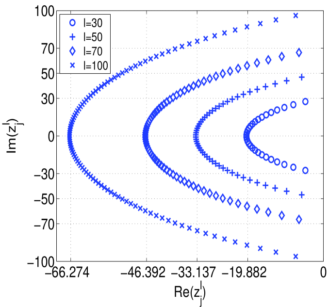
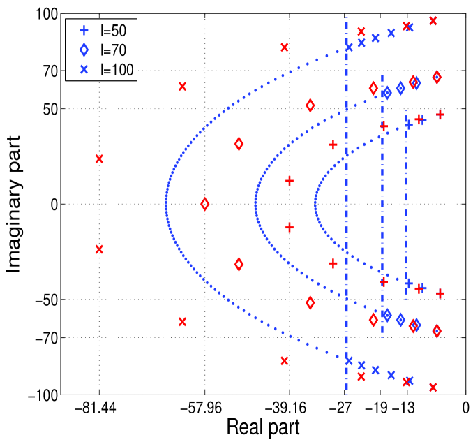
Figure 1: Left: distributions of the zeros of $K_{l+1/2}(z).$ Right: distributions of poles in [2](red color), and used zeros (blue color), which lies on the right of the vertical dashdot line $-\beta la$ with $\beta=0.4.$

Armed with the explicit formulas (9)-(10), we can compute the NRBKs at any time. Observe that as the real part of $z_{j}^{l}$ is negative, $e^{\frac{c}{b}z_{j}^{l}t}$ becomes exponentially small when $z_{j}^{l}$ is far away from the imaginary axis and $t$ is slightly large. This motivates us to drop many insignificant zeros by using the algorithm described in [19] (see Figure 1 (right)).

C.  Fast algorithms for temporal convolution.

Observe from (9)-(10) that the time variable $t$ only appears in the exponentials. This allows for a fast recursive temporal convolution as shown in [2]. More precisely, given a generic function $g(t)$, we define

$$f(t;r):=e^{\frac{c}{b}rt}\ast g(t)=\int_{0}^{t}e^{\frac{c}{b}r(t-\tau)}g(\tau)\,d\tau,$$ (11)

and find

$$f(t+\Delta t;r)=e^{\frac{c}{b}r\Delta t}f(t;r)+\int_{t}^{t+\Delta t}e^{\frac{c}{b}r(t+\Delta t-\tau)}g(\tau)\,d\tau,$$ (12)

where $\Delta t$ is the time step size. We see that at each time step, the computation narrows down to computing the integral of the current interval $[t,t+\Delta t].$ This essentially eliminates the burden of history dependence induced by the temporal convolution.

Using this notion, we deduce from (9)-(11) that

$$[\sigma_{l}\ast g](t)=\frac{c}{b}\sum_{j=1}^{l}z_{j}^{l}\int_{0}^{t}e^{\frac{c}{b}z_{j}^{l}(t-\tau)}g(\tau)d\tau=\frac{c}{b}\sum_{j=1}^{l}z_{j}^{l}f(t;z_{j}^{l}),$$ (13)

$$[\omega_{l}\ast g](t)=\frac{c}{b}\sum_{j=1}^{l}(z_{j}^{l})^{2}\int_{0}^{t}e^{\frac{c}{b}z_{j}^{l}(t-\tau)}g(\tau)d\tau+g(t)\sum_{j=1}^{l}z_{j}^{l}=\frac{c}{b}\sum_{j=1}^{l}(z_{j}^{l})^{2}f(t;z_{j}^{l})+g(t)\sum_{j=1}^{l}z_{j}^{l}.$$ (14)

Given $g$ at grids for time discretization, we only need to store $\{f(t;z_{j}^{l})\}_{j=1}^{l}$ for previous steps to compute the convolutions at current time. It is optimal for storage requirement.

D.  Summary of the algorithm.

For clarity, we summarize the whole algorithm and outline two strategies to further reduce the complexity related to large $l.$ The algorithm is intended to compute ${\mathcal{T}}_{b}[\boldsymbol{E}](t)$ in (7) at $t=t_{n}=n\Delta t,n\geq 0,$ and on the colatitude-longitude grids adopted by the Spherepack [1] from $\boldsymbol{E}$ on the same grids. —————————————————————————————————————————–

Algorithm for computing ${\mathcal{T}}_{b}[\boldsymbol{E}]$ in (7)

• Step 1.  Use the Spherepack to compute $\big{\{}{E}_{lm}^{r},{E}_{lm}^{(1)}\big{\}}$ from $\boldsymbol{E}.$

• Step 2.  Compute the zeros $\{z_{j}^{l}\}$ for $l\geq 1.$

• Step 3.  Compute $\sigma_{l}\ast{E}_{lm}^{(2)}$ and $\omega_{l}\ast{E}_{lm}^{r}$ via (13)-(14).

• Step 4.  Use the Spherepack to compute ${\mathcal{T}}_{b}[\boldsymbol{E}]$ via (7).

—————————————————————————————————————————–

It is clear that the number of zeros to be used is determined by the truncation of the expansion (2). If $l$ is large, we can adopt the strategies (i) dropping insignificant zeros (cf. [19]) and (ii) compression algorithm (cf. [2]) to reduce the complexity in Step 3. Here, we outline the main idea.

• Since $e^{\frac{c}{b}z_{j}^{l}t}$ becomes exponentially small when $z_{j}^{l}$ is far away from the imaginary axis and $t$ is slightly large, for some $t_{0}^{l}>0,$ we modify the NRBKs $\sigma_{l}$ and $\omega_{l}$ in (9)-(10) as follows

  $$\tilde{\sigma}_{l}(t)=\frac{c}{b}\sum_{j\in\Upsilon_{l}^{\beta}}z_{j}^{l}e^{\frac{c}{b}z_{j}^{l}t},\quad\tilde{\omega}_{l}(t)=\frac{c}{b}\sum_{j\in\Upsilon_{l}^{\beta}}(z_{j}^{l})^{2}e^{\frac{c}{b}z_{j}^{l}t}+\delta(t)\sum_{j=1}^{l}z_{j}^{l},\;\;t>t_{0}^{l},$$ (15)

  where $\Upsilon_{l}^{\beta}=\big{\{}z_{j}^{l}\,:\,{\rm Re}(z_{j}^{l})\geq-\beta la\big{\}}$ with $a\approx 0.66742$ and $\beta\in(0,1)$ ( $\beta$ tunes the number of used zeros). We plot in Figure 1 (right) the used zeros for $\beta=0.4$. This can reduce the zeros from $100$ to $10$ (see the marker ‘$\times$’ on the right of vertical dashdot line) and leads to quite accurate approximation. We refer to the analysis in [19] on how to adjust $\beta$ and $t_{0}^{l}$ to achieve a good accuracy.

• Alpert et al. [2] proposed a compression technique by a rational approximation of the NRBK in $s$-domain, which required to solve a nonlinear least square problem. This led to the approximate poles $\{\tilde{z}_{j}^{d}\}_{j=1}^{d}$ with $d\ll l$ (see Figure 1 (right, marked by ‘$\times$’) with a reduction from $l=100$ to $d=12$ and error tolerance $10^{-8}$). Correspondingly, $\sigma_{l}$ and $\omega_{l}$ could be approximated by

  $$\hat{\sigma}_{l}(t)=\frac{c}{b}\sum_{j=1}^{d}\alpha_{j}^{d}e^{\frac{c}{b}\tilde{z}_{j}^{d}t},\;\;\hat{\omega}_{l}(t)=\frac{c}{b}\sum_{j=1}^{d}\alpha_{j}^{d}\tilde{z}_{j}^{d}e^{\frac{c}{b}\tilde{z}_{j}^{d}t}+\delta(t)\sum_{j=1}^{d}\alpha_{j}^{d},\quad t>0,$$ (16)

  where $\{\alpha_{j}^{d}\}_{j=1}^{d}$ are the coefficients occurring in the rational partial fraction: $\alpha_{j}^{d}/(s-c\tilde{z}_{j}^{d}/b).$ Some samples of $\{\alpha_{j}^{d},\tilde{z}_{j}^{d}\}_{j=1}^{d}$ are available from the website: http://faculty.smu.edu/thagstrom/sph6.txt.

3.  Numerical Results and Discussions

In this section, we provide some numerical examples to show the accuracy of computing the NRBC. We also test a spectral-Galerkin with (second-order) Newmark’s time integration for Maxwell’s equations in a spherical shell $\{a<|\boldsymbol{x}|<b\}$, where the NRBC is set at the outer spherical surface $r=b$.

In the following tests, we generate the exact solution through the field: $(\boldsymbol{\hat{x}}\times\boldsymbol{E})|_{r=a}=\boldsymbol{g}$, and with homogeneous initial data and source term. More precisely, we take

$${\boldsymbol{g}}(\theta,\phi,t)=\sum_{l=1}^{\infty}\sum_{m=-l}^{l}\bigg{[}\sin^{6}(6t)\,g_{l,1}^{m}\,\nabla_{S}Y_{l}^{m}+\bigg{(}\mathcal{L}^{-1}\bigg{[}\frac{c}{sa}+\frac{k^{\prime}_{l}(sa/c)}{k_{l}(sa/c)}\bigg{]}(t)\ast\sin^{8}(4t)\bigg{)}\,g_{l,2}^{m}\,{\boldsymbol{T}}_{l}^{m}\bigg{]},$$

where $\{g_{l,1}^{m},g_{l,2}^{m}\}$ are the expansion coefficients in terms of $\{\nabla_{S}Y_{l}^{m},{\boldsymbol{T}}_{l}^{m}\},$ of the the function

$${\tilde{\boldsymbol{g}}}(\theta,\phi)=b\bigg{(}\,\Big{(}\cos\big{(}x_{1}^{2}x_{2}x_{3}\big{)}+2\Big{)}^{\frac{5}{2}},x_{3}^{2}\Big{(}\sin\big{(}x_{1}x_{2}\big{)}+1\Big{)}^{\frac{3}{2}},x_{1}\Big{(}0.5\cos\big{(}x_{2}x_{3}\big{)}+1\Big{)}^{\frac{7}{2}}\,\bigg{)}.$$

Note that $\boldsymbol{x}=(x_{1},x_{2},x_{3})$ (with $|\boldsymbol{x}|=1$) is the corresponding Cartesian coordinates. Here, we compute $\{g_{l,1}^{m},g_{l,2}^{m}\}$ accurately by using the Spherepack [1].

We first test the accuracy of the algorithm for the NRBC (3). Let ${\boldsymbol{E}}^{\boldsymbol{N}}$ be the truncated exact solution $\boldsymbol{E}$ (the included modes are $1\leq l\leq N_{\theta};|m|\leq l$). Define the error:

$$e(b,t)=\Big{\|}\Big{(}\partial_{t}{\boldsymbol{E}}^{\boldsymbol{N}}_{T}-c\,\boldsymbol{\hat{x}}\times(\nabla\times{\boldsymbol{E}}^{\boldsymbol{N}})\Big{)}-{\mathcal{T}}_{b}[{\boldsymbol{E}}^{\boldsymbol{N}}]\Big{\|}_{N_{\theta},N_{\phi}},$$ (17)

where $\|\cdot\|_{N_{\theta},N_{\phi}}$ denotes the discrete $L^{2}$-norm associated with $N_{\theta}\times N_{\phi}$ colatitude and longitude grids. Here, we take $a=2,c=5,N_{\theta}=40$ and $N_{\phi}=2N_{\theta}$. We aim to test the accuracy for computing ${\mathcal{T}}_{b}[{\boldsymbol{E}}^{\boldsymbol{N}}],$ so the differentiations in $t$ and curl are calculated analytically. In Table 1, we tabulate $e(b,t)$ for different $t$ and $b$ (note: the magnitude of $\boldsymbol{E}$ is actually between $1$ and $20$, so the waves cross the artificial boundary). We see that in all cases, the computation of the NRBC is very accurate.

Table 1: The error $e(b,t)$ for different $t$ and $b$

$t$	$b=3$	$b=5$	$b=5$	$b=6$
1.0	7.73246E-14	2.67652E-14	1.64591E-14	1.10549E-14
2.0	7.01963E-14	4.43072E-14	4.30850E-14	9.58167E-14
4.0	1.30672E-13	7.07636E-14	8.15754E-14	9.56271E-14
10.0	3.35293E-13	1.87063E-13	2.32403E-13	2.74720E-13

Next, we set the NRBC as the boundary condition and solve the Maxwell’s equation in curl-curl formulation with homogeneous initial conditions and free source in a spherical shell. In this case, we can expand the interior electric field in VSHs, and reduce the problem to a sequence of equations in radial direction. Then we solve the systems by using the spectral-Galerkin method in space and the second-order Newmark scheme in time. Moreover, we use the Richardson extrapolation to improve the time discretization to fourth-order. We refer to [19] for similar idea for the acoustic wave equations, and report the details in the extended version.

Under the same setting of the reference solution and other data, we provide in Table 2, the discrete $L^{2}$-norm errors (in space with sufficient resolution): $\text{Err(}t\text{)}$ (Newmark scheme), $\text{Err${}^{\text{R}}$(}t\text{)}$ (Richardson extrapolation), and the convergence order in time at different time $t$. As expected, we observe the second-order convergence for the Newmark scheme and the fourth-order convergence for the extrapolation.

Table 2: Convergence of the Newmark scheme and Richardson extrapolation.

$t$	$\Delta t$	Err	order	Err${}^{\text{R}}$	order	$t$	$\Delta t$	Err	order	Err${}^{\text{R}}$	order
	5.00e-3	2.3090E-2		2.0719E-5			5.00e-3	1.6912E-2		2.8491E-5
	2.50e-3	5.7684E-3	2.001	1.2870E-6	4.009		2.50e-3	4.2193E-3	2.003	1.7754E-6	4.004
0.5	1.25e-3	1.4419E-3	2.000	8.0317E-8	4.002	1.5	1.25e-3	1.0543E-3	2.000	1.1088E-7	4.001
	1.00e-3	9.2276E-4	2.000	3.2912E-8	3.998		1.00e-3	6.7470E-4	2.001	4.5411E-8	4.009
	5.00e-3	2.1041E-2		2.6540E-5			5.00e-3	2.2117E-2		2.3189E-5
	2.50e-3	5.2591E-3	2.000	1.6500E-6	4.008		2.50e-3	5.5142E-3	2.004	1.4467E-6	4.003
1.0	1.25e-3	1.3147E-3	2.000	1.0299E-7	4.001	2.0	1.25e-3	1.3776E-3	2.001	9.0376E-8	4.001
	1.00e-3	8.4140E-4	2.000	4.2178E-8	4.009		1.00e-3	8.8159E-4	2.000	3.7016E-8	4.000

We have proposed in this paper an efficient algorithm for computing the spherical NRBC for the Maxwell’s equations. This tool can be integrated well with various interior solvers in bounded domain for simulating scattering problems in many situations. We will report the works along this line in the forthcoming papers.

References

- [1] J.C. Adams and P.N. Swarztrauber. Spherepack 3.0: A model development facility. Monthly Weather Review, 127(8):1872–1878, 1999.
- [2] B. Alpert, L. Greengard, and T. Hagstrom. Rapid evaluation of nonreflecting boundary kernels for time-domain wave propagation. SIAM J. Numer. Anal., 37(4):1138–1164 (electronic), 2000.
- [3] J.P. Berenger. A perfectly matched layer for the absorption of electromagnetic waves. J. Comput. Phys., 114(2):185–200, 1994.
- [4] Z.M. Chen and J.-C. Nédélec. On Maxwell equations with the transparent boundary condition. J. Comput. Math., 26(3):284–296, 2008.
- [5] R.D. Ciskowski and C.A. Brebbia. Boundary Element Methods in Acoutics. Kluwer Academic Publishers, 1991.
- [6] T. Hagstrom. Radiation boundary conditions for the numerical simulation of waves. In Acta numerica, 1999, volume 8 of Acta Numer., 47–106. Cambridge Univ. Press, Cambridge, 1999.
- [7] T. Hagstrom and S. Lau. Radiation boundary conditions for Maxwell’s equations: a review of accurate time-domain formulations. J. Comput. Math., 25(3):305–336, 2007.
- [8] J.B. Keller and D. Givoli. Exact nonreflecting boundary conditions. J. Comput. Phys., 82(1):172–192, 1989.
- [9] J.F. Lee and Z. Sacks. Whitney elements time domain (WETD) methods. IEEE Transactions on Magnetics, 31(3):1325–1329, 1995.
- [10] J.R. Li. Low order approximation of the spherical nonreflecting boundary kernel for the wave equation. Linear Algebra Appl., 415(2-3):455–468, 2006.
- [11] Y. Lin, J.H. Lee, J. Liu, M. Chai, J.A. Mix, and Q.H. Liu. A hybrid SIM-SEM method for 3-D electromagnetic scattering problems. IEEE Transactions on Antennas and Propagation, 57(11):3655–3663, 2009.
- [12] Q.H. Liu. The PSTD algorithm: A time-domain method requiring only two cells per wavelength. Microwave and Optical Technology Letters, 15(3):158–165, 1998.
- [13] C. Lubich and A. Schädle. Fast convolution for nonreflecting boundary conditions. SIAM J. Sci. Comput., 24(1):161–182 (electronic), 2002.
- [14] P.M. Morse and H. Feshbach. Methods of Theoretical Physics. 2 volumes. McGraw-Hill Book Co., Inc., New York, 1953.
- [15] J.C. Nédélec. Acoustic and Electromagnetic Equations, volume 144 of Applied Mathematical Sciences. Springer-Verlag, New York, 2001. Integral representations for harmonic problems.
- [16] D. Nicholls and J. Shen. A rigorous numerical analysis of the transformed field expansion method. SIAM J. Numer. Anal., 47(4):2708–2734, 2009.
- [17] I.L. Sofronov. Conditions for complete transparency on a sphere for a three-dimensional wave equation. Dokl. Akad. Nauk, 326(6):953–957, 1992.
- [18] A. Taflove and S.C. Hagness. Computational Electrodynamics: the Finite-Difference Time-Domain Method. Artech House Inc., Boston, MA, third edition, 2005.
- [19] L.-L. Wang, B. Wang, and X.D. Zhao. Fast and accurate computation of time-domain acoustic scattering problems with exact nonreflecting boundary conditions. SIAM J. Appl. Math., 72(6):1869–1898, 2012.
- [20] G.N. Watson. A Treatise of the Theory of Bessel Functions (second edition). Cambridge University Press, Cambridge, UK, 1966.